Deep-Learning Convolutional Neural Networks for scattered shrub detection with Google Earth Imagery

Abstract

There is a growing demand for accurate high-resolution land cover maps in many fields, e.g., in land-use planning and biodiversity conservation. Developing such maps has been performed using Object-Based Image Analysis (OBIA) methods, which usually reach good accuracies, but require a high human supervision and the best configuration for one image can hardly be extrapolated to a different image. Recently, the deep learning Convolutional Neural Networks (CNNs) have shown outstanding results in object recognition in the field of computer vision. However, they have not been fully explored yet in land cover mapping for detecting species of high biodiversity conservation interest. This paper analyzes the potential of CNNs-based methods for plant species detection using free high-resolution Google Earth^TM images and provides an objective comparison with the state-of-the-art OBIA-methods. We consider as case study the detection of Ziziphus lotus shrubs, which are protected as a priority habitat under the European Union Habitats Directive. According to our results, compared to OBIA-based methods, the proposed CNN-based detection model, in combination with data-augmentation, transfer learning and pre-processing, achieves higher performance with less human intervention and the knowledge it acquires in the first image can be transferred to other images, which makes the detection process very fast. The provided methodology can be systematically reproduced for other species detection.

Index terms— object detection, Ziziphus lotus, plant species detection, convolutional neural network (CNN), object-based image analysis (OBIA), remote sensing

1 Introduction

Changes in land cover and land use are pervasive, rapid, and can have significant impact on humans, the economy, and the environment. Accurate land cover mapping is of paramount importance in many applications, e.g., in urban planning, forestry, natural hazard mapping, habitat mapping, assessment of land-use change effects on climate, etc. [8, 24].

In practice, land cover maps are built by analyzing remotely sensed imagery, captured by satellites, airplanes or drones, using different classification methods. The accuracy of the results and their interpretation depends on the quality of the input data, e.g., spatial, spectral, and radiometric resolution of the images, and also on the classification methods used. The most used methods can be divided into two categories: pixel-based classifiers and Object-Based Image Analysis (OBIA) [4]. Pixel-based methods, which use only the spectral information available for each pixel, are faster but ineffective especially for high resolution images [19, 21]. Object-based methods take into account the spectral as well as the spatial properties of image objects, i.e., set of neighbor similar pixels.

OBIA methods are more accurate but very expensive from a computational point of view, they require a high human supervision and number of iterations to obtain acceptable accuracies, and are not easily portable to other images (e.g., to other areas, seasons, extensions, radiometric calibrations or different spatial or spectral resolutions). To detect a specific object in an input image, first, the OBIA method segments the image (e.g., by using a multi-resolution segmentation algorithm), and then classifies the segments based on their similarities (e.g., by using algorithms such as the k-nearest neighbor). This procedure has to be repeated for each single input image and the knowledge acquired from one input image cannot be reutilized in another.

In the last five years, deep learning and particularly supervised Convolutional Networks (CNNs) based models have demonstrated impressive accuracies in object recognition and image classification in the field of computer vision [14, 17, 11, 25]. This success is due to the availability of larger datasets, better algorithms, improved network architectures, faster GPUs and also improvement techniques such as, transfer-learning and data-augmentation.

This paper analyzes the potential of CNNs-based methods for plant species mapping using high-resolution Google Earth^TM images and provides an objective comparison with the state-of-the-art OBIA-based methods.

As case study, this paper addresses the challenging problem of detecting Ziziphus lotus shrubs, a species known by its role as the dominant plant that characterizes an ecosystem of priority conservation in the European Union “Arborescent matorral” with Ziziphus, which is experiencing a serious decline during the last decades. The complexity of this case is due to the fact that Ziziphus lotus individuals are scattered arborescent shrubs with variable shapes, sizes, and distribution patterns. In addition, distinguishing Ziziphus lotus shrubs from other neighbor plants in remote sensing images is complex for non-experts and for automatic classification methods.

From our results, compared to OBIA, the detection model based on GoogLeNet network, in combination with data-augmentation, transfer-learning (fine-tuning) and pre-processing the input test images, achieves higher precision and balance between recall and precision in the problem of Ziziphus lotus detection. In addition, the detection process using GoogLeNet detector is faster, which implies a high user productivity in comparison with OBIA.

In particular, the contributions of this work are:

• Developing an accurate CNN-based detection model for plant individuals mapping using high-resolution remote sensing images, extracted from Google Earth^TM.

• Designing a new dataset containing images of Ziziphus lotus individuals and bare soil with sparse vegetation for training the CNNs-based model.

• Demonstrating that the use of small datasets to train GoogLeNet-model with transfer learning from ImageNet (i.e., fine-tuning) can lead to satisfactory results that can be further enhanced by including data-augmentation, and specific pre-processing techniques.

• Comparing a CNN-based model with an OBIA-based method in terms of performance, user productivity, and transferability to other regions.

• Providing a complete description of the used methodology so that it can be reproduced by other researchers for the classification and detection of other plant species.

This paper is organized as follows. A review of related works is provided in Section 2. A description of the proposed CNN-methodology is given in Section 3. The considered study areas and how the dataset were constructed to train the CNN-based classifier can be found in Section 4. The experimental results of the detection using CNNs and OBIA are provided in Section 5 and finally conclusions.

2 Related Works

This section reviews the related work in land cover mapping then explains how OBIA, the state-of-the-art methods are used for plant species detection.

2.1 Land cover mapping

In the field of remote sensing, object detection has been traditionally performed using pixel-based classifiers or object-based methods [21]. Several papers have demonstrated that Object-Based Image Analysis (OBIA) methods are more accurate than pixel based methods, particularly for high spatial resolution images [4]. In the field of computer vision, object detection within an image is more challenging than scene tagging or classification because it is necessary to determine the image segment that contains the searched object. In most object detection works, first a classifier is trained and then it is run either on a number of sliding windwos or on the segmented input image.

Recently, deep learning CNNs have started to be used for scene tagging and object detection in remotely sensed images [33, 16, 13, 26]. However, as far as we know, there does not exist any study on using CNNs in plant species detection or comparison between OBIA and deep CNNs methods.

The existing works that use deep CNNs in remotely sensed images can be divided into two broad groups. The first group focuses on the object detection or classification of high-resolution multi-band imagery, i.e., with a spectral dimension greater than three, and apply CNNs-based methods at the pixel level, i.e., using only the spectral information [33, 16]. The second group focuses on the classification or tagging of whole aerial RGB images, commonly called scene classification, and show their accuracies using bechmark databases such as, UC-Merced dataset  and Brazilian Coffee Scenes dataset  [6, 13]. It is worth to mention that these datasets contain a large number of manually labeled images. For example, the Brazilian Coffee Scenes dataset contains $50,000$ of $64\times 64$-pixel tiles, labeled as coffee (1,438) non-coffee (36,577) or mixed (12,989) and UC-Merced dataset contains 2100 $256\times 256$-pixel images labeled as belonging to 21 land use classes, 100 images corresponding to each class. Several works have reached classification accuracies greater than $95\%$ on these database  [6, 13].

The most related work to ours is [18]. It addresses the detection of palm oil trees in agricultural areas using four bands imagery with $0.5\times 0.5$m spatial resolution via CNNs. Since oil-palm trees have the same age, shape, size, and are placed at the same distance from each other, the authors could combine LeNet-based classifier with a very simple detecting technique. In addition, the authors used a large number of manually labeled training samples, 5000 palm tree samples and 4000 background samples.

Our study is more challenging, because Ziziphus lotus is not a crop, it is a wild plant that has very different shapes, sizes, and intensities of the green color. In addition, we will show in this paper that a smaller training set can also lead to competitive results.

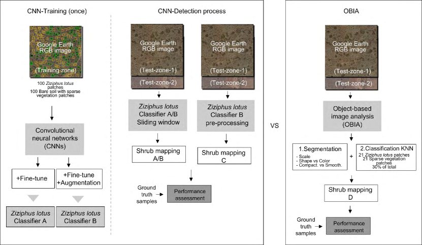
(a) CNN                          (b) OBIA

Figure 1: Flowchart of the Ziziphus lotus shrub mapping process using (a) Convolutional neural networks (CNNs), considering two detection approaches: slidning window and pre-processing and (b) Object-based image analysis (OBIA).

2.2 OBIA-based detection

Differently to CNNs-based approach, OBIA-based detector does not re-utilize the learning from one image to another. The detection is applied from scratch on each individual image. The OBIA detection approach is performed in two steps. First, the input image is segmented, and then each segment is analyzed by a classification algorithm. A simplistic flowchart of the CNNs- and OBIA-based approaches is illustrated in Figure 1(b). The OBIA-detector used in this study is implemented in E-cognition 8.9 software [12] and works in two steps as follows:

• Segmentation step: first, the input image is segmented using the multi-resolution algorithm [2]. In this step, the user has to manually initialize a set of non-dimensional parameters namely: i) The scale parameter, to define the maximum standard deviation of the homogeneity criteria (in color and shape) in regard to the weighted images layers for resulting image objects. The higher the value, the larger the resulting image objects. ii) The shape versus color parameter, to prioritize homogeneity in color versus in shape or texture when creating the image objects. Values closer to one indicate shape priority, while values closer to zero indicate color priority. iii) The compactness versus smoothness parameter, to prioritize whether producing compact objects over smooth edges during the segmentation. Values closer to one indicate compactness priority, while values closer to zero indicate smoothness priority [30].

• Classification step: the resulting segments are classified using the K-Nearest Neighbor (KNN) method. For this, the user identifies sample sites for each class and calculates their statistics. Then, objects are classified based on their resemblance to the training sites using the calculated statistics. Finally, the validation of the classification is carried out using an independent set of field samples. KNN typically uses 30% of labeled field samples for training, i.e. calculating the statistics, and 70% of the field samples to evaluate the classifier. It provides a confusion matrix to calculate the commission and omission errors, and the overall accuracy [7].

3 CNN-based detection for plant species mapping

We reformulate the problem of detecting a particular plant species into a two-class problem, where the true class is “Ziziphus lotus shrubs” and the false class is “bare soil with sparse vegetation”. To build the CNNs-based detection model, we first designed a field-validated training dataset, then we built a classification model (CNN classifier), and finally, during the detection process, we considered two solutions, the sliding-window technique and a set of pre-processing techniques to localize Ziziphus lotus in the test scenes. A simplistic flowchart of the CNNs- and OBIA-based approaches is illustrated in Figure 1(a).

3.1 Classification model using fine-tuning

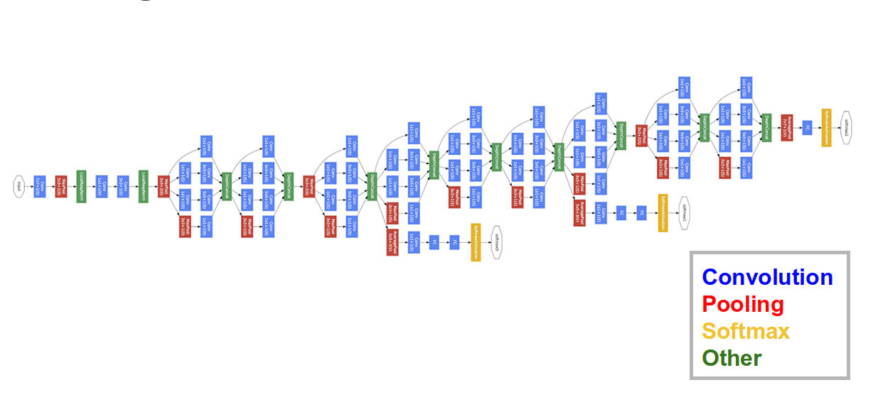
Figure 2: Architecture of GoogLeNet network [28].

In this work, we use feed-forward Convolutional Neural Networks (CNNs) for supervised classification, as they have provided very good accuracies in several applications. These methods automatically discover increasingly higher level features from data [14, 10]. The lower convolutional layers capture low-level image features, e.g. edges, color, while higher convolutional layers capture more complex features, i.e., composite of several features.

We use GoogLeNet model [28], which was the winner of ILSVRC (ImageNet Large Scale Visual Recognition Competition (ILSVRC)) 2014. Compared with previous network architectures, GoogLeNet provides higher accuracy with less computational cost. It has 12$\times$ fewer parameters than AlexNet, the network that won ILSVRC 2012. GoogLeNet has 6.8 million parameters and 22 layers with learnable weights organized in four parts: i) the initial segment, made up of three convolutional layers, ii) nine inception modules, each module is a set of convolutional and pooling layers at different scales performed in parallel then concatenated together, iii) two auxiliary classifiers, each classifier is actually a smaller convolutional network put on the top of the output of an intermediate inception module, and iv) one output classifier. See Figure 2.

Deep CNNs, such as Googlenet, are generally trained based on the prediction loss minimization. Let $x$ and $y$ be the input images and corresponding output class labels, the objective of the training is to iteratively minimize the average loss defined as

$$J(w)=\frac{1}{N}\sum_{i=1}^{N}L(f(w;x_{i}),y_{i})+\lambda R(w)$$ (1)

This loss function measures how different is the output of the final layer from the ground truth. $N$ is the number of data instances (mini-batch) in every iteration, $L$ is the loss function, $f$ is the predicted output of the network depending on the current weights $w$, and R is the weight decay with the Lagrange multiplier $\lambda$. It is worth to mention that in the case of GoogLeNet, the losses of the two auxiliary classifiers are weighted by $0.3$ and added to the total loss of each training iteration. The Stochastic Gradient Descent (SGD) is commonly used to update the weights.

$$w_{t+1}=\mu w_{t}-\alpha\Delta J(w_{t})$$ (2)

where $\mu$ is the momentum weight for the current weights $w_{t}$ and $\alpha$ is the learning rate.

The network weights, $w_{t}$, can be randomly initialized if the network is trained from scratch. However, this is suitable only when a large labeled training-set is available, which is expensive in practice. Several works have shown that data-augmentation [29] and transfer learning [27] help overcoming this limitation.

• Transfer learning (e.g. fine-tuning in CNNs) consists of re-utilizing the knowledge learnt from one problem to another related one ([20]). Applying transfer learning with deep CNNs depends on the similarities between the original and new problem and also on the size of the new training set. In deep CNNs, transfer learning can be applied via fine-tuning, which involves initializing the weights of the network by the pre-trained weights on a different dataset.

  In general, fine-tuning the entire network, i.e., updating all the weights, is only used when the new dataset is large enough, otherwise, the model could suffer overfitting especially among the first layers of the network. Since these layers extract low-level features, e.g., edges and color, they do not change significantly and can be utilized for several visual recognition tasks. The last learnable layers of the CNN are gradually adjusted to the particularities of the problem and extract high level features.

  In this work, we have used fine-tuning GoogleNet and initialized it with the pre-trained weights of the same architecture on ImageNet dataset (around 1.28 million images over 1,000 generic object classes) [14].

• Data-augmentation, also called data transformation or distortion, it is used to increase the volume of the training set by applying specific deformations on the input images, e.g., rotation, translation. The set of transformations that improves the performance of the CNN-model depends on the particularities of the problem.

3.2 Plant species detection

To obtain an accurate detection in a new image, different from the image used for training the CNN-classifier, we analyzed two approaches:

• Sliding window is a technique frequently used for detection. The detection task consists of applying the obtained GoogLeNet-classifier at all locations and scales of the input image. The sliding window approach is an exhaustive method since it considers a very large number of candidate windows of different sizes and shapes across the input image. The classifier is then run on each one of these windows. To maximize the detection accuracy, the probabilities obtained from different window sizes can be assembled into one heatmap. Finally, probability heatmaps are usually transformed into classes using a thresholding technique, i.e., areas with probabilities higher than 50% are usually classified as the true class (e.g. Ziziphus lotus) and areas with probabilities lower than 50% as background (e.g. bare soil with sparse vegetation).

• Pre-processing techniques can also help to improve the detection accuracy and execution time. The set of pre-processing techniques that provides the best results depends on the nature of the problem and the object of interest. From the multiple techniques that we explored, the ones that provided the best detection performance were: i) Eliminating the background using a threshold based on its typical color or darkness (e.g. by converting the RGB image to gray scale, grays lighter than 100 digital level corresponded to bare ground). ii) Applying an edge-detection method that filters out the objects with an area or perimeter smaller than the minimum size of the target objects (e.g. 180 pixels of resolution $0.5\times 0.5$ m, correspond to the area of the smallest Ziziphus lotus individual in the image, around 22 m²).

4 Study areas and datasets construction

This Section describes the study areas and provides full details on how the training and test sets were built using Google Earth^TM images. We consider the challenging problem of detecting Ziziphus lotus shrubs, since this is the key species of an ecosystem of priority conservation in the European Union (habitat 5220* habitat of 92/43/EEC Directive) that is declining during the last decades in SE Spain, Sicily, and Cyprus, where the only European populations occur ([32]). In Europe, the largest population occurs in the Cabo de Gata-Níjar Natural Park (SE Spain), where an increased mortality of individuals of all ages has been observed in the last decade ([9]).

4.1 Study areas

In this study, we considered three zones: one training-zone, for training the CNN-model, and two test zones (labeled as test-zone-1 and test-zone-2) for testing and comparing the performance of both CNN- and OBIA-based models.

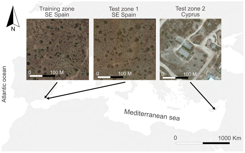
Figure 3: Localization of the three study areas used in this work: Training-zone and Test-zone-1 in Cabo de Gata-Níjar Natural Park (Spain), and Test-zone-2 in Rizoelia National Forest Park (Cyprus). The three images are $230\times 230$ m with a native resolution in Google Earth^TM of 0.5 m per pixel (but downloaded as $1900\times 1900$ pixel images). Ziziphus lotus shrubs can be seen in the three images. The used projection was geographic with the WGS84 Datum.

• The training-zone used for training the CNN-based model. This zone is located in Cabo de Gata-Níjar Natural Park, 36^∘49’43” N, 2^∘17’30” W, in the province of Almería, Spain (Figure 3). The climate is semi-arid Mediterranean. The vegetation is scarce and patchy, mainly dominated by large Ziziphus lotus shrubs surrounded by a heterogeneous matrix of bare soil and small scrubs (e.g. Thymus hyemalis, Launea arborescens and Lygeum spartum) with low coverage ([32, 23]). Ziziphus lotus forms large hemispherical bushes with very deep roots and 1-3 m tall that trap and accumulate sand and organic matter building geomorphological structures, called nebkhas, that constitute a shelter micro-habitat for many plant and animal species ([32, 31, 15]).

• Test-zone-1 and test-zone-2 belong to two different protected areas. Test-zone-1 is located $1.5$ km west from the training-zone, 36^∘49’45” N, 2^∘17’30” W. Test-zone-2 is located in Rizoelia National Forest Park in Cyprus, 34^∘56’08” N, 33^∘34’27” (Figure 3). These two test-zones are used for comparing the performance between CNNs and OBIA for detecting Ziziphus lotus.

4.2 Datasets construction

In OBIA, the training dataset consists of a set of georreferenced points from each one of the classes that we want to classify. These points must fall in the same scene that we aim to classify. Conversely, for CNNs, the training dataset consists of a set of images that contain the object of interest, but these images do not have to belong to same scene that we aim to classify, allowing for transferability to other regions, which is an advantage of CNNs over the OBIA method.

The satellite RGB orthoimages used were downloaded from Google Earth^TM in WGS84 Mercator (sphere radius 6378137 m, European Petroleum Survey Group (EPSG) 3785). The scenes of the three areas, training-zone, test-zone-1 and test-zone-2, are of size $230\times 230$ meters. The images were downloaded using the maximum zoom level in their area. The obtained scenes have $1900\times 1900$ pixels, with a pixel size of 0.12 m due to the smoothing applied by Google Earth at the highest zoom, however the real resolution is approximately 0.5 m. The capturing date was June 22th 2016 for the two zones in Spain, and June 20th 2015 for Cyprus.

We addressed the Ziziphus lotus detection problem by considering two classes, 1) Ziziphus lotus shrubs class and 2) Bare soil with sparse vegetation class.

4.2.1 Datasets for training OBIA and for ground truthing

• In test-zone-1, from Spain, 72 Ziziphus lotus individuals were identified in the field. The perimeter of each was georeferenced in the field with a differential GPS, GS20, Leica Geosystems, Inc. From the 72 individuals, 30% (21 individuals) were used for training the OBIA method and 70% (51 individuals) as ground truth both for the OBIA and the CNN method.

• In test-zone-2, from Cyprus, 41 Ziziphus lotus individuals were visually identified in Google Earth by the authors using descriptions provided by local experts ([5]). From the 41 individuals, 30% (12 individuals) were used for training the OBIA method and 70% (29 individuals) as ground truth both for the OBIA and the CNN method. In both test zones, the corresponding number of points (72 and 41, respectively) were georeferenced for the Bare soil with sparse vegetation class.

4.2.2 Training dataset for the CNN-classifier

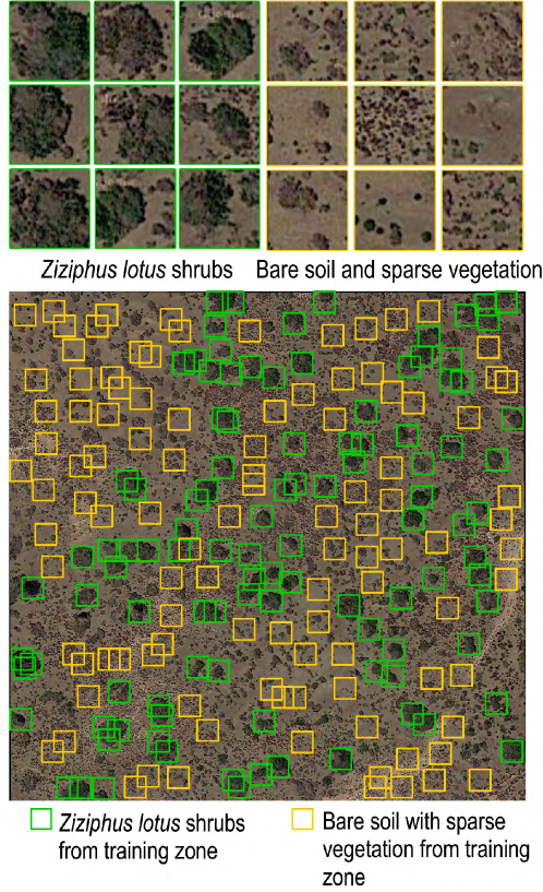
Figure 4: The two top panels show examples of the $80\times 80$-pixels image patches used to build the training dataset for the CNN model: left) patches of Ziziphus lotus class, right) patches of Bare soil with sparse vegetation class. The bottom panel shows the training-zone dataset with Ziziphus lotus patches labeled with a green contour and Bare soil and sparse vegetation patches labeled with yellow contour.

The design of the training dataset is key to the performance of a good CNN classification model. For labeling the training dataset, we identified 100 $80\times 80$-pixels image patches containing Ziziphus lotus shrubs and 100 images for Bare soil with sparse vegetation. Examples of the labeled classes can be seen in Figure 4. We distributed the 100 images of each class into 80 images for training and 20 images for validating the obtained CNNs classifiers, as summarized in Table 1.

Table 1: Training and testing datasets for both CNN (Convolutional Neural Networks) and OBIA (Object-Based Image Analysis) used for mapping Ziziphus lotus shrubs. Bare soil: Bare soil and sparse vegetation; Img: 80x80-pixel images; Poly: digitized polygons

Class	CNN Classifier		OBIA classifier		Accuracy
	training	validation	training		assessment
	Training-zone		Test-zone-1	Test-zone-2	Test-zone-1	Test-zone-2
Ziziphus	80 img	20 img	21 poly	15 poly	51 poly	36 poly
Bare soil	80 img	20 img	21 poly	15 poly	51 poly	36 poly

5 Experimental evaluation and accuracy assessment

This section is organized in two parts. The first part describes the steps taken to improve the baseline detection results of the CNN-based model (GoogLeNet). In particular, we considered transfer-learning (fine-tuning) and data-augmentation to improve the classifier training, and selecting the best sliding-window size and pre-processing (background elimination and long-edge detection) to improve the classifier detection performance. The second part describes the classification steps used with OBIA and provides a comparison between GoogeLeNet- and OBIA-models. For the evaluation and comparison of accuracies, we used three metrics, precision (also called positive predictive value, i.e., how many detected Ziziphus are true), recall (also known as sensitivity, i.e., how many actual Ziziphus were detected), and F1 measure, which evaluates the balance between precision and recall. Where

$$precision=\frac{True~{}Positives}{True~{}Positives+False~{}Positives},$$

$$recall=\frac{True~{}Positives}{True~{}Positives+False~{}Negatives},$$

and

$$F1~{}measure=2\times\frac{precision\times recall}{precision+recall}$$

5.1 CNN training with fine-tuning and augmentation

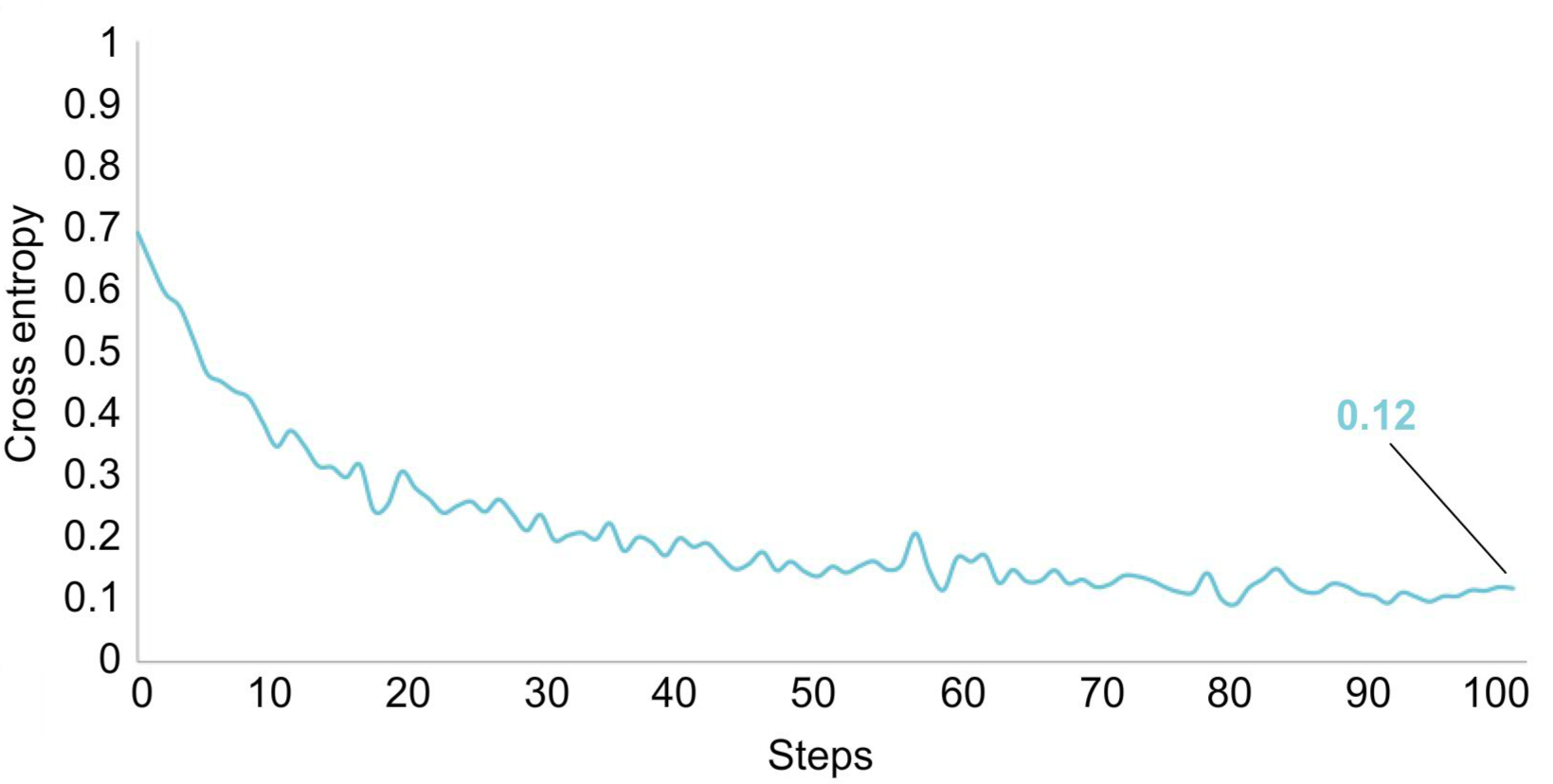
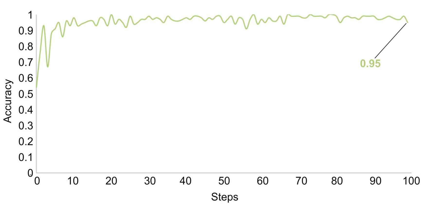
Figure 5: The accuracy and cross entropy of the GoogLeNet-classifier with fine-tuning and data-augmentation during the training process of Ziziphus lotus shrubs with Google Earth images.

For the experiments with GoogleNet-based model, we have used the open source software library Tensorflow ([1]). To improve the accuracy and reduce overfitting we i) used fine-tuning by initializing the model with the pre-trained weights of ImageNet, and ii) applied data augmentation techniques to increase the size of the dataset from 100 to 6000 images. In particular, we applied:

• Random scale: increases the scale of the image by a factor picked randomly in [1 to 10%]

• Random crop: crops the image edges by a margin in [0 to 10%]

• Flip horizontally: randomly mirrors the image from left to right.

• Random brightness: multiplies the brightness of the image by a factor picked randomly in [0, 10].

The obtained classifier converges within the first 100 training iterations as shown in Figure 5.

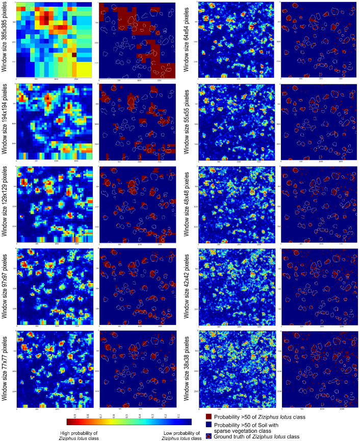
Figure 6: Maps showing the probability of Ziziphus lotus presence according to the GoogLeNet-classifier trained with fine-tuning and data-augmentation and applied on different sliding-window sizes from $38\times 38$ to $385\times 385$ pixels in Test-zone-1. The first and third columns show the heatmaps of the probability of Ziziphus lotus presence, and the second and fourth columns show the corresponding binary maps after applying a threshold of probability greater than 50%. The white polygons correspond to the ground-truth perimeter of each individual georeferenced in the field with a differential GPS.

5.1.1 Detection with Sliding windows

Table 2: The CNN-detection results in Test-zone-1 with different sliding window sizes. Accuracies are expressed in terms of true positives (TP), false positives (FP) and false negatives (FN), precision, recall, F1-measure, and execution time of the detection process.

win. size	total # of	TP	FP	FN	precis.	recall	F1-	time
(pixels)	win.				(%)	(%)	meas.(%)	(min)
385$\times$385	196	31	18	41	63.27	43.06	51.24	6.0
194$\times$194	961	34	7	38	82.93	47.22	60.18	29.4
129$\times$129	2209	42	6	30	87.50	58.33	70.00	67.6
97$\times$ 97	4096	59	6	13	90.77	81.94	86.13	125.4
77$\times$77	5929	59	5	13	92.19	81.94	86.76	181.5
64$\times$64	9506	65	7	7	90.28	90.28	90.28	291.0
55$\times$55	13340	65	12	7	84.42	90.28	87.25	408.4
48$\times$48	17292	68	16	4	80.95	94.44	87.18	529.3
42$\times$42	22200	70	17	2	80.46	97.22	88.05	679.6
38$\times$ 38	27888	71	39	1	64.55	98.61	78.02	853.7

To assess the ability of CNNs model to detect Ziziphus lotus shrubs in Google Earth images, we applied the trained GoogLeNet classifier across the entire scene of test-zone-1 by using the sliding window technique. Since the diameter of the smallest Ziziphus lotus individual georeferenced in the field was 4.6 m ($38$ pixels) and the largest individual in the region has a diameter of 47 m ($385$ pixels), we evaluated a range of window sizes between $38\times 38$ and $385\times 385$ pixels and a horizontal and vertical sliding step of about $70\%$ the size of the sliding window, e.g., $27\times 27$ pixels for the $38\times 38$ sliding window, and $269\times 269$ pixels for $385\times 385$ sliding window.

The performance of the GoogLeNet-based detector on the $1900\times 1900$ pixels image corresponding to test-zone-1 are shown in Table 2 and the corresponding heatmap to each window size are illustrated in Figure 6. The best accuracies, highest recall and F1-measure and high precision, were obtained for a window size of $64\times 64$ pixels. The time needed to perform the detection process using this window size was $291$ minutes. This represents the execution time that would be required for Ziziphus lotus shrub detection on any new input image of the same dimensions, which is time consuming to be used in larger regions or across the entire range distribution of the species along the Mediterranean region. To reduce the execution time we next explored the use of appropriate pre-processing techniques.

Table 3: The GoogLeNet CNN-detection results for Ziziphus lotus shrub mapping in Test-zone-1 with and without data-augmentation, both under the sliding window approach, and using pre-processing. Accuracies are expressed in terms of true positives (TP), false positives (FP), false negatives (FN), precision, recall, and F1 measure. The highest accuracies are highlighted in bold.

Detection model	TP	FP	FN	precision	recall	F1
CNNs (test-zone-1)
+fine-tuning
+sliding window	63	12	9	84.00%	87.50%	85.71%
+ CNNs (test-zone-1)
+fine-tuning
+augmentation
+sliding window	65	7	7	90.28%	90.28%	90.28%
CNNs (test-zone-1)
+fine-tuning
+augmentation
+pre-processing	69	1	3	98.57%	95.83%	97.18%

5.1.2 Detection with image pre-processing

To optimize the CNN-detection accuracy and execution time, we analyzed the impact of several pre-processing techniques. It is worth to mention that the set of pre-processing techniques that provides the best results depends on the nature of the problem and the object of interest. From the multiple techniques explored, the ones that improved the performance of the detector in this work were: i) Eliminating the background using a threshold based on the high albedo (light color) of the bare soil. For this, we first converted the RGB image to gray scale and then created a binary mask-band to select only those pixels darker than 100 over 256 digital levels of gray, which was the average level of gray of the field georeferenced polygons of bare soil in test-zone-1. ii) Applying an edge-detection method to the previously created mask-band to select only clusters of pixels with an area greater than 180 pixels (21.6 m²), which approximately was the size of the smallest Ziziphus lotus individual georeferenced in test-zone-1. After pre-processing, the number of candidate image patches to pass to the CNN detector was 78 for test-zone-1 and 53 for test-zone-2, what significantly decreased the detection computing time. See illustration of the pre-processing phase in Figure 7.

The results of the CNN-based detection, considering all the optimizations in the training and detection steps described above for test-zone-1 are summarized in Table 3. The CNN model reached relatively good accuracies ($>84\%$) using only fine-tuning and very good accuracies when adding data-augmentation ($>90\%$) under the sliding-window detection approach. Using pre-processing techniques together with fine-tuning and data-augmentation clearly improved the precision, recall and F1 by $14.57\%$, $8.33\%$ and $11.47\%$, respectively, compared with the baseline CNN-model with fine-tuning and under the sliding window approach.

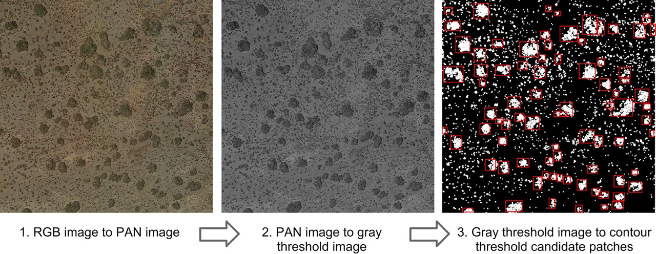
Figure 7: Pre-processing consisted in, first, converting the three band image into one gray-scale band image (PAN), second, converting the gray-scale image into a binary image based on a 100 over 256 digital value threshold, and third, detecting Ziziphus lotus shrubs only in pixels with a digital value greater than 100. The 78 candidate patches identified in Test-zone-1 are labeled with red contour in the right panel (the 53 candidates in Test-zone-2 are not shown.

Table 4: A comparison between GoogLeNet and OBIA-based detectors, on test-zone-2, in terms of true positives (TP), false positives (FP), false negatives (FN), precision , recall and F1_measure. The highest values are highlighted in bold.

Detection model	TP	FP	FN	precision	recall	F1
CNNs (test-zone-1)
+fine-tuning
+augmentation
+pre-processing	69	1	3	98.57%	95.83%	97.18%
OBIA (test-zone-1)	66	19	6	77.65%	91.67%	84.08%
CNNs (test-zone-2)
+fine-tuning
+augmentation
+pre-processing	38	3	3	92.68%	92.68%	92.68%
OBIA (test-zone-2)	21	8	20	72.41%	51.00%	60.00%

5.2 CNN- versus OBIA-detector

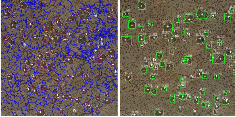
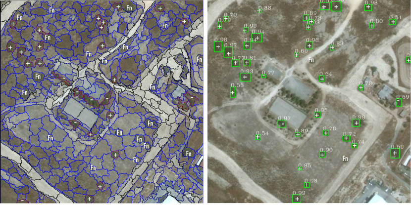
(a) OBIA detection on test-zone-1    (b)CNN detection on test-zone-1 (c) OBIA detection on test-zone-2    (d) CNN detection on test-zone-2

Figure 8: The detection results obtained by OBIA-based model on test-zone-1 (a) and test-zone-2 (c) and CNN-based model on test-zone-1 (b) and test-zone-2 (d). The symbols (+), (-) and (Fn) stand for true positive, false positive and false negative respectively. The values on the top of the bounding boxes in (2) and (4) show the probabilities, calculated by GoogLeNet-detector, of having a Ziziphus lotus shrubs.

To obtain the best detection results using OBIA-method, the user has to manually determine the best segmentation parameters and classification procedure. In this work, we iteratively tried all possible combinations among parameters: scale ranging in $[80,160]$ at intervals of 5, shape and compactness ranging in $[0.1,0.9]$ at intervals of 0.1. An exhaustive search of the best configuration implied the evaluation of $2511$ combinations, each segmentation test took $18$ seconds, and each classification test took around $10$ seconds. The whole detection process using OBIA took around $12.5$ hours. The best segmentation parameters were: scale = 110, shape $=0.3$, compactness $=0.8$. The best classification configuration was: Brightness $<80.87$, Red Band $>97.35$, Green Band $<81.18$, Blue Band $<64.96$ and gray level co-occurrence matrix (GLCM mean) $<80.54$. To ensure a fair comparison with CNNs, we re-utilized the segmentation and classification configuration from test-zone-1 in test-zone-2. It is important to recall that OBIA requires the user to provide training points of each input class located within the scene to classify.

To test the performance of the CNN classifier in a region with different characteristics and far away from the training zone, we compared the performance of GoogLeNet-based model and the OBIA-method in test-zone-1 in Spain and test-zone-2 in Cyprus (results summarized in Table 3). As we can observe from these tables, CNN-based detection model achieved significantly better detection results than OBIA on both test zones. On test-zone-1, CNN achieves higher precision, 98.57% versus 77.65%, higher recall, 95.83% versus 91.67%, and higher F1-measure, 95.83% versus 84.08% than OBIA. Similarly, on test-zone-2, CNN achieves significantly better precision, recall and F1-measure than OBIA. The detection results of CNN and OBIA, on test-zone-1, are shown in Figure 8(1) and (2) and on test-zone-2 are shown in Figure 8(3) and (4).

In terms of user productivity, the training of the CNN-classifier with fine-tuning and data augmentation were performed only once and took 7.55 minutes on two NVIDIA GeForce GTX 980 GPUs. In the deploying phase, using GoogLeNet-classifier and pre-processing on test-zone-1 and test-zone-2 took 35.4 and 24.1 seconds respectively. Whereas, finding the best configuration for OBIA on each test-zone took around 12.5 hours. Applying the obtained CNN-detector to any new image of similar sizes will take seconds; however, applying OBIA to a new image will take 12.5 hours. This clearly shows that the user becomes more productive with CNNs.

6 Conclusions

In this work, we explored, analyzed and compared two detection methodologies, the OBIA-based approach and the CNNs-based approach, in the challenge of mapping Ziziphus lotus, a shrub of priority conservation interest in Europe. Our experiments demonstrated that the GoogLeNet-based classifier with transfer learning from ImageNet and data augmentation, together with pre-processing techniques provided better detection results than OBIA-based methods. In addition, a very competitive advantage of the CNN-based detector is that it required less human supervision than OBIA and can be easily ported to other regions or scenes with different characteristics, i.e., color, extent, light, seasons.

The proposed CNN-based approach can be systematized and reproduced in a wide variety of object detection problems or land-cover mapping using Google Earth images. For instance, our CNN-based approach could support the detection and monitoring of trees and arborescent shrubs, which has a huge relevance for biodiversity conservation and carbon accounting worldwide. The presence of scattered trees have been recently highlighted as keystone structures capable of maintaining high levels of biodiversity and ecosystem services provision in open areas [22]. Global initiatives could greatly benefit from the CNNs, such as those recently implemented by the United Nations Food and Agricultural Organization [3] to estimate the overall extension of forests in drylands biomes, where they used the collaborative work of hundreds of people that visually explored hundreds of VHR images available from Google Earth to detect the presence of forests in drylands.

References

- [1] M. Abadi, A. Agarwal, P. Barham, E. Brevdo, Z. Chen, C. Citro, G.S. Corrado, A. Davis, J. Dean, M. Devin, et al. Tensorflow: Large-scale machine learning on heterogeneous distributed systems. arXiv preprint arXiv:1603.04467, 2016.
- [2] M. Baatz, A. Schäpe, et al. Multiresolution segmentation: an optimization approach for high quality multi-scale image segmentation. Angewandte geographische informationsverarbeitung XII, 58:12–23, 2000.
- [3] J.F. Bastin, N. Berrahmouni, A. Grainger, D. Maniatis, D. Mollicone, R. Moore, C. Patriarca, N. Picard, B. Sparrow, E.M. Abraham, et al. The extent of forest in dryland biomes. Science, 356(6338):635–638, 2017.
- [4] T. Blaschke. Object based image analysis for remote sensing. ISPRS journal of photogrammetry and remote sensing, 65(1):2–16, 2010.
- [5] D.M. Browning, S.R. Archer, and A.T. Byrne. Field validation of 1930s aerial photography: What are we missing? Journal of Arid Environments, 73(9):844–853, 2009.
- [6] M. Castelluccio, G. Poggi, C. Sansone, and L. Verdoliva. Land use classification in remote sensing images by convolutional neural networks. arXiv preprint arXiv:1508.00092, 2015.
- [7] R.G. Congalton and K. Green. Assessing the accuracy of remotely sensed data: principles and practices. CRC press, 2008.
- [8] R.G. Congalton, J. Gu, K. Yadav, P. Thenkabail, and M. Ozdogan. Global land cover mapping: A review and uncertainty analysis. Remote Sensing, 6(12):12070–12093, 2014.
- [9] E. Guirado Hernandez. Factores que afectan a la distribucion especial de vegetacion freatofita (zipiphus lotus) en el acuifero costero de torre garcia (sureste de españa). Master thesis, 2015.
- [10] Y. Guo, Y. Liu, A. Oerlemans, S. Lao, S. Wu, and M.S. Lew. Deep learning for visual understanding: A review. Neurocomputing, 187:27–48, 2016.
- [11] G. Hinton, L. Deng, D. Yu, G. Dahl, N. Mohamed, A.and Jaitly, A. Senior, V. Vanhoucke, P. Nguyen, T. Sainath, and B. Kingsbury. Deep Neural Networks for Acoustic Modeling in Speech Recognition: The Shared Views of Four Research Groups. IEEE Signal Process. Mag., 29(6):82–97, 2012.
- [12] http://www.ecognition.com. Ecognition. -, last access 5th may 2017.
- [13] F. Hu, G. Xia, J. Hu, and L. Zhang. Transferring deep convolutional neural networks for the scene classification of high-resolution remote sensing imagery. Remote Sensing, 7(11):14680–14707, 2015.
- [14] A. Krizhevsky, I. Sutskever, and G. E. Hinton. Imagenet classification with deep convolutional neural networks. In Advances in neural information processing systems, pages 1097–1105, 2012.
- [15] F. Lagarde, T. Louzizi, T. Slimani, H. El Mouden, K.B. Kaddour, S. Moulherat, and X. Bonnet. Bushes protect tortoises from lethal overheating in arid areas of morocco. Environmental Conservation, 39(02):172–182, 2012.
- [16] M. Längkvist, A. Kiselev, M. Alirezaie, and A. Loutfi. Classification and segmentation of satellite orthoimagery using convolutional neural networks. Remote Sensing, 8(4):329, 2016.
- [17] Quoc V. Le. Building high-level features using large scale unsupervised learning. In 2013 IEEE Int. Conf. Acoust. Speech Signal Process., pages 8595–8598, 2013.
- [18] W. Li, H. Fu, L. Yu, and A. Cracknell. Deep learning based oil palm tree detection and counting for high-resolution remote sensing images. Remote Sensing, 9(1):22, 2016.
- [19] X. Li and G. Shao. Object-based land-cover mapping with high resolution aerial photography at a county scale in midwestern usa. Remote Sensing, 6(11):11372–11390, 2014.
- [20] S. J. Pan and Q. Yang. A survey on transfer learning. IEEE Transactions on knowledge and data engineering, 22(10):1345–1359, 2010.
- [21] K.B. Pierce. Accuracy optimization for high resolution object-based change detection: An example mapping regional urbanization with 1-m aerial imagery. Remote Sensing, 7(10):12654–12679, 2015.
- [22] J. A. Prevedello, M. Almeida-Gomes, and D.B. Lindenmayer. The importance of scattered trees for biodiversity conservation: a global meta-analysis. Journal of Applied Ecology, In press.
- [23] S. Rivas Goday and F. Bellot. Las formaciones de zizyphus lotus (l.) lamk., en las dunas del cabo de gata. Anal. Inst. Esp. Edaf. Fisiol. Veg, 3:109–126, 1944.
- [24] John Rogan and DongMei Chen. Remote sensing technology for mapping and monitoring land-cover and land-use change. Progress in planning, 61(4):301–325, 2004.
- [25] T. N. Sainath, A. Mohamed, B. Kingsbury, and B. Ramabhadran. Deep convolutional neural networks for LVCSR. In 2013 IEEE Int. Conf. Acoust. Speech Signal Process., pages 8614–8618, 2013.
- [26] A. Santara, K. Mani, P. Hatwar, A. Singh, A. Garg, K. Padia, and P. Mitra. Bass net: Band-adaptive spectral-spatial feature learning neural network for hyperspectral image classification. arXiv preprint arXiv:1612.00144, 2016.
- [27] H. Shin, H. R. Roth, M. Gao, L. Lu, Z. Xu, I. Nogues, J. Yao, D. Mollura, and R. M. Summers. Deep convolutional neural networks for computer-aided detection: Cnn architectures, dataset characteristics and transfer learning. IEEE transactions on medical imaging, 35(5):1285–1298, 2016.
- [28] Christian Szegedy, Wei Liu, Yangqing Jia, Pierre Sermanet, Scott Reed, Dragomir Anguelov, Dumitru Erhan, Vincent Vanhoucke, and Andrew Rabinovich. Going deeper with convolutions. In Proceedings of the IEEE Conference on Computer Vision and Pattern Recognition, pages 1–9, 2015.
- [29] S. Tabik, D. Peralta, A. Herrera-Poyatos, and F. Herrera. A snapshot of image pre-processing for convolutional neural networks: case study of mnist. International Journal of Computational Intelligence Systems, 10:555–568, 2017.
- [30] J Tian and D-M Chen. Optimization in multi-scale segmentation of high-resolution satellite images for artificial feature recognition. International Journal of Remote Sensing, 28(20):4625–4644, 2007.
- [31] R. Tirado. 5220 matorrales arborescentes con ziziphus. VV. AA. Bases ecológicas preliminares para la conservación de los tipos de hábitat de interés comunitario en Espana. Ministerio de Medio Ambiente, Medio Rural y Marino. Madrid, 68, 2009.
- [32] R. Tirado and F.I. Pugnaire. Shrub spatial aggregation and consequences for reproductive success. Oecologia, 136(2):296–301, 2003.
- [33] W. Zhao, S. Du, and W.J. Emery. Object-based convolutional neural network for high-resolution imagery classification. IEEE Journal of Selected Topics in Applied Earth Observations and Remote Sensing, 2017.