Analyzing Random Permutations for Cyclic Coordinate Descent

Abstract.

We consider coordinate descent methods for minimization of convex quadratic functions, in which exact line searches are performed at each iteration. (This algorithm is identical to Gauss-Seidel on the equivalent symmetric positive definite linear system.) We describe a class of convex quadratic functions for which the random-permutations version of cyclic coordinate descent (RPCD) is observed to outperform the standard cyclic coordinate descent (CCD) approach on computational tests, yielding convergence behavior similar to the fully-random variant (RCD). A convergence analysis is developed to explain the empirical observations.

1. Introduction

The coordinate descent (CD) approach for solving the problem

(1.1) $$\min\,f(x),\quad\mbox{where $f:\mathbb{R}^{n}\to\mathbb{R}$ is smooth and convex,}$$

follows the framework of Algorithm 1. We denote

(1.2) $$\nabla_{i}f(x)=[\nabla f(x)]_{i},\quad e_{i}=(0,\dotsc,0,1,0,\dotsc,0)^{T},$$

where the single nonzero in $e_{i}$ appears in position $i$. Epochs (indicated by the counter $\ell$) encompass cycles of inner iterations (indicated by $j$). At each iteration $k$, one component of $x$ is selected for updating; a steplength parameter $\alpha_{k}$ is applied to the negative gradient of $f$ with respect to this component.

  Set Choose $x^{0}\in\mathbb{R}^{n}$;

  for $\ell=0,1,2,\dotsc$ do

     for $j=0,1,2,\dotsc,n-1$ do

        Define $k=\ell n+j$;

        Choose index $i=i(\ell,j)\in\{1,2,\dotsc,n\}$;

        Choose $\alpha_{k}>0$;

        $x^{k+1}\leftarrow x^{k}-\alpha_{k}\nabla_{i}f(x^{k})e_{i}$;

     end for

  end for

Algorithm 1 Coordinate Descent

The choice of coordinate $i=i(\ell,j)$ to be updated at inner iteration $j$ of epoch $\ell$ differs between variants of CD, as follows:

• For “cyclic CD” (CCD), we choose $i(\ell,j)=j+1$.

• For “fully randomized CD,” also known as “stochastic CD,” and abbreviated as RCD, we choose $i(\ell,j)$ uniformly at random from $\{1,2,\dotsc,n\}$ and independently at each iteration.

• For “random-permutations CD” (abbreviated as RPCD), we choose $\pi_{\ell+1}$ at the start of epoch $\ell$ to be a random permutation of the index set $\{1,2,\dotsc,n\}$ (chosen uniformly at random from the space of random permutations), then set $i(\ell,j)$ to be the $(j+1)$th entry in $\pi_{\ell+1}$, for $j=0,1,2,\dotsc,n-1$.

Note that $x^{ln}$ denotes the value of $x$ after $l$ epochs.

We consider in this paper problems in which $f$ is a strictly convex quadratic, that is

(1.3) $$f(x)=\frac{1}{2}x^{T}Ax,$$

with $A$ symmetric positive definite. Even this restricted class of functions reveals significant diversity in convergence behavior between the three variants of CD described above. The minimizer of (1.3) is obviously $x^{*}=0$. Although (1.3) does not contain a linear term, it is straightforward to extend our results to the case for problems of the form

$$f(x)=\frac{1}{2}x^{T}Ax-b^{T}x$$

by replacing $x^{0}$ in several places of our analysis with $x^{0}-x^{*}$, where $x^{*}=A^{-1}b$ is the minimizer of this problem. We assume that the choice of $\alpha_{k}$ in Algorithm 1 is the exact minimizer of $f$ along the chosen coordinate direction. The resulting approach is thus equivalent to the Gauss-Seidel method applied to the linear system $Ax=0$. The variants CCD, RCD, RPCD can be interpreted as different cyclic / randomized variants of Gauss-Seidel for this system.

In the RPCD variant, we can express a single epoch as follows. Letting $P$ be the permutation matrix corresponding to the permutation $\pi$ on this epoch, we split the symmetrically permuted Hessian into strictly triangular and diagonal parts as follows:

(1.4) $$P^{T}AP=L_{P}+\Delta_{P}+L_{P}^{T},$$

where $L_{P}$ is strictly lower triangular and $\Delta_{P}$ is diagonal. We then define

(1.5) $$C_{P}:=-(L_{P}+\Delta_{P})^{-1}L_{P}^{T},$$

so that the epoch indexed by $l-1$ can be written as follows:

(1.6) $$x^{ln}=(P_{l}C_{P_{l}}P_{l}^{T})x^{(l-1)n},$$

where $P_{l}$ denotes the matrix corresponding to permutation $\pi_{l}$. By recursing to the initial point $x^{0}$, we obtain after $\ell$ epochs that

(1.7) $$x^{\ell n}=(P_{\ell}C_{P_{\ell}}P_{\ell}^{T})(P_{\ell-1}C_{P_{\ell-1}}P_{\ell-1}^{T})\dotsc(P_{1}C_{P_{1}}P_{1}^{T})x^{0},$$

yielding a function value of

(1.8) $$f(x^{\ell n})=\frac{1}{2}(x^{0})^{T}\left((P_{1}C_{P_{1}}^{T}P_{1}^{T})\dotsc(P_{\ell}C_{P_{\ell}}^{T}P_{\ell}^{T})A(P_{\ell}C_{P_{\ell}}P_{\ell}^{T})\dotsc(P_{1}C_{P_{1}}P_{1}^{T})\right)x^{0}.$$

We analyze convergence in terms of the expected value of $f$ after $\ell$ epochs for any given $x^{0}$, with the expectation taken over the permutations $P_{1},P_{2},\dotsc,P_{\ell}$, that is,

(1.9) $$\mathbb{E}_{P_{1},P_{2},\dotsc,P_{\ell}}\,f(x^{\ell n}).$$

1.1. Previous Work

Convergence of RCD is analyzed in [5], showing that when the objective is strongly convex, the method requires $O((nL_{\max}/\mu)|\log\hat{\epsilon}|)$ iterations to reach an objective function value that is within $\hat{\epsilon}$ of the optimal value, in expectation, when the coordinates are sampled in a uniform random manner, where $\mu$ is the modulus of strong convexity and $L_{\max}$ is the maximum coordinate-wise Lipschitz constant for the gradient. This rate can be improved to $O((nL_{\text{avg}}/\mu)|\log\hat{\epsilon}|)$ if the sampling probability for each coordinate is proportional to the coordinate-wise Lipschitz constants, where $L_{\text{avg}}$ is the average of these constants. On the other hand, the best known convergence rate of CCD for convex quadratic problems, given by [8], has an iteration complexity for reaching an $\hat{\epsilon}$-accurate solution deterministically that can be $O(n^{2})$ times slower than that for RCD in the worst case. The best worst-case convergence guarantees for RPCD so far are still identical to those for CCD. (The analyses for CCD assume only that each coordinate is processed exactly once per epoch, and are indifferent to the fact that the ordering of coordinates can change on each epoch, as in RPCD.) However, in practice it is sometimes observed that RPCD behaves in a manner more similar to RCD than CCD (see, for example, the experiments in [7] and the talks [11, 12]), and a rigorous explanation for the general convergence rate for the expected objective of RPCD over the random permutations has been difficult to obtain. Some trials have been conducted to tackle this problem. Recht and Ré [6] state a conjecture whose consequence is that RPCD converges faster than RCD on quadratic problems, but they prove the result only for some special random cases. Sun et al. [10] have analyzed the convergence speed of the distance between the expected iterate $\mathbb{E}[x^{k}]$ and the minimizer $x^{*}$ for convex quadratic problems, but this cannot be translated to a result for the expected squared error $\mathbb{E}\|x^{k}-x^{*}\|^{2}$ nor the expected function suboptimality $\mathbb{E}(f(x^{k})-f(x^{*}))$, which are much more informative quantities.

Computational experience reported in [11, 12] showed that for most convex quadratic functions (1.3), the convergence behaviors of all variants of CD are similar. For example, when $A$ is a matrix of the form $V\Sigma V^{T}$ where $V$ is random orthogonal and $\Sigma$ is a positive diagonal matrix whose diagonals (the eigenvalues of $A$) follow a log-uniform distribution, then CCD, RCD, and RPCD all converge at roughly the same rates, no matter how widely the eigenvalues are dispersed. However, these computational tests revealed a class of matrices $A$ for which the variants had radically different performance: matrices of the form

(1.10) $$A=\delta V\Sigma V^{T}+(1-\delta)\mathbf{1}\mathbf{1}^{T},$$

for small positive values of $\delta$, and $\mathbf{1}=(1,1,\dotsc,1)^{T}$. For such matrices, the performance of RCD and RPCD is similar, but CCD converges much more slowly. In this paper, we explain much of this anomalous behavior by considering a matrix closely related to (1.10), and explaining the difference by means of a specialized analysis of RPCD.

The current paper is an extension of our paper [3] in which, motivated by the empirical observation above, we considered the special case of (1.10) in which $\Sigma=I$, that is,

(1.11) $$A:=\delta I+(1-\delta)\mathbf{1}\mathbf{1}^{T},\quad\mbox{where $\delta\in(0,n/(n-1))$.}$$

It was proved by [8] that this matrix achieves worst-case convergence behavior for CCD. We showed in [3] that a factor of $O(n^{2})$ fewer iterations are required by RPCD to achieve the same accuracy, and that the complexity of RPCD is similar to RCD in this case. Salient properties of the matrix (1.11) include the following.

• It has eigenvalue $\delta$ replicated $(n-1)$ times, and a single dominant eigenvalue $\delta+(1-\delta)n$, and

• it is invariant under symmetric permutations, that is, $P^{T}AP=A$ for all permutation matrices $P$.

The latter property makes the analysis of RPCD much more straightforward than for more general $A$ of the form (1.10). Specifically, it follows from (1.5) that $C_{P}\equiv C=-(L+\Delta)^{-1}L^{T}$, where $A=L+\Delta+L^{T}$, that is, $C_{P}$ is independent of $P$. For the matrix (1.11), the expression (1.6) thus simplifies to

$$x^{ln}=(P_{l}CP_{l}^{T})x^{(l-1)n},\quad l=1,2,3,\dotsc.$$

We refer to [3] for a more extensive discussion of prior related work on variants of coordinate descent. We note in particular that for general convex functions $f$, CCD has weaker convergence guarantees than for convex quadratic $f$, as analyzed in [1, 9, 4]. By contrast, the convergence results for RCD presented in [5] show no difference between quadratic and nonquadratic convex functions.

1.2. Contributions

In this work, we study the behavior of the RPCD variant of CD on problems of the form (1.3), where the coefficient matrix has the form

(1.12) $$B_{u}:=\delta I+(1-\delta)uu^{T},$$

for some $u\in\mathbb{R}^{n}$. This paper focuses on the case in which the components of $u$ are not too different in magnitude, and are all close to $1$. Rather than working directly with (1.12), we work with a diagonally scaled version that has a form more tractable for analysis. By scaling (1.12) symmetrically with the matrix $U=\operatorname{diag}(u)$, we obtain

$$A_{\epsilon}:=\delta I+(1-\delta)\mathbf{1}\mathbf{1}^{T}+\epsilon D,$$

(1.13) where $$\delta\in(0,n/(n-1)) \epsilon\geq 0$$, ,

$$D=\operatorname{diag}(d) \min_{i}d_{i}=0 \max_{i}d_{i}=1$$, with and .

(Details are given in Section 2.) Note that both forms (1.12) and (1.13) are generalizations of (1.11). They are both closely related to the more general form (1.10), in that (1.12) can be obtained from (1.10) by a symmetric scaling with $\Sigma^{-1/2}V$, while (1.13) has the form (1.10) with $V=I$ and $\Sigma=I+(\epsilon/\delta)D$. Thus, this paper provides a significantly more complete explanation of the anomalous convergence behavior involving matrices (1.10) than our earlier work.

For matrices of the form (1.13) in (1.3), this paper proves similar convergence behavior for RPCD to what was proved in [3] for the special case (1.11), in the regime defined by the following values of the parameters $n$, $\epsilon$, and $\delta$:

(1.14) $$0<\delta\leq\epsilon,\quad\left|\rho_{1}\right|\epsilon^{2}<\delta\ll 1,\quad n\epsilon\leq 1.$$

where $\rho_{1}$ is a positive or negative quantity of modest size, magnitude not much larger than $1$, and independent of $n$, $\epsilon$, and $\delta$. We prove that the convergence rate guarantee of RPCD for problems defined by (1.13) is similar to that of RCD, and much better than the rate bound for CCD. Specifically, we explain via analysis of a linear recurrence that captures the epoch-wise behavior of RPCD that the per-epoch objective improvement is bounded by a factor of approximately

(1.15) $$1-1.4\delta,$$

which is similar to the corresponding factors of approximately $1-\delta$ and $1-2\delta$ that are known for RCD (by different analyses), and significantly better than the factor of approximately $(1-\delta/n^{2})$ arising from worst-case theoretical guarantees for CCD. By the generalization of (1.11) to (1.13) (and thus (1.12)), we extend our understanding of the empirical behavior of RPCD, RCD, and CCD described at the beginning of Section 1.1.

1.3. Remainder of the Paper

In Section 2, we relate matrices of the forms (1.13) and (1.12), showing that the behavior of CD is similar on both. Section 3 presents our analysis for the behavior of RPCD on problem (1.3), (1.13). In particular, we define a sequence of matrices $\{\bar{A}_{\epsilon}^{(t)}\}$ such that given any initial guess $x^{0}$, the expected value of the objective $f(x^{tn})$ after the $t$th epoch is $\tfrac{1}{2}(x^{0})^{T}\bar{A}_{\epsilon}^{(t)}x^{0}$. We then define a sequence of matrices $\{\hat{A}_{\epsilon}^{(t)}\}$ that dominates $\{\bar{A}_{\epsilon}^{(t)}\}$, and that can be parametrized compactly. We analyze convergence of the sequence $\{\hat{A}_{\epsilon}^{(t)}\}$ by means of a spectral analysis of the matrix that relates its parameters at successive values of $t$, and use it to develop an estimate of the asymptotic per-epoch improvement of the objective $f(x^{tn})$, $t=0,1,2,\dotsc$. We provide an explanation in Section 3.5 for the large decrease in $f$ that is often observed in the very first iteration of CD, a phenomenon that is not explained by the asymptotic analysis. Section 4 discusses RCD and CCD variants for the problem (1.3), (1.13), while Section 5 reports computational experience with the three variants.

1.4. Notation

In addition to the notation $\rho_{1}$ mentioned above, which denotes a scalar quantity of size not much greater than $1$ and independent of $n$, $\epsilon$, and $\delta$, we make extensive use of vector quantities $\mathbf{r_{1}}\in\mathbb{R}^{n}$ and matrix quantities $\mathbf{R_{1}}\in\mathbb{R}^{n\times n}$ (symmetric in some contexts and nonsymmetric in others), which we assume are both bounded in norm by $1$, that is,

(1.16) $$\|\mathbf{r_{1}}\|\leq 1,\quad\|\mathbf{R_{1}}\|\leq 1.$$

In the case in which $\mathbf{R_{1}}$ is also symmetric, it follows from these assumptions that $-I\preceq\mathbf{R_{1}}\preceq I$. This notation is essential to capturing remainder terms that appear in our analysis. In particular, it allows us to keep explicit track of dependence of the remainder terms on $n$, $\epsilon$, and $\delta$. For example, a vector quantity whose size is bounded by a modest multiple of $\epsilon^{2}n^{-1}$ can be represented by $\rho_{1}\epsilon^{2}n^{-1}\mathbf{r_{1}}$. The following estimate follows immediately from this notation:

(1.17) $$\mathbf{R_{1}}v\mathbf{1}^{T}=\rho_{1}\mathbf{r_{1}}\mathbf{1}^{T}\;\;\mbox{provided $\|v\|\leq\rho_{1}$}.$$

Matrix and vector norms $\|\cdot\|$ signify $\|\cdot\|_{2}$ throughout, unless some other subscript is specified.

2. Quadratic functions with Hessians of the form (1.13)

We discuss here the matrix of the form (1.13), explaining its relationship to (1.12) and to (1.11), and giving some preliminaries for the analysis of RPCD on the corresponding quadratic function.

2.1. Relating (1.13) to (1.12)

Given $\epsilon>0$ and $\delta\in(0,1)$, suppose that $u\in\mathbb{R}^{n}$ satisfies

(2.1) $$\min_{i=1,2,\dotsc,n}\,|u_{i}|=\sqrt{\frac{\delta}{\delta+\epsilon}},\quad\max_{i=1,2,\dotsc,n}\,|u_{i}|=1.$$

Consider the matrix $B_{u}$ from (1.12). Defining $U:=\operatorname{diag}(u)$, we have

(2.2) $$A_{\epsilon}:=U^{-1}B_{u}U^{-1}=\delta U^{-2}+(1-\delta)\mathbf{1}\mathbf{1}^{T},$$

and note that the diagonal elements of $U^{-2}$ are in the range $[1,\epsilon/\delta+1]$. Thus we can write $\delta U^{-2}=\delta I+\epsilon D$, where $D$ is diagonal with elements in $[0,1]$, so in fact $A_{\epsilon}$ in (2.2) has the form (1.13).

We verify in Appendix A that the iterates generated by Algorithm 1 for a given sequence of indices $i(\ell,j)$ to (1.3) with $A=B_{u}$ from (1.12), and with starting point $\tilde{x}^{0}$ and exact line search are isomorphic to the iterates generated by applying the same algorithm with the same index sequence to (1.3) with $A=A_{\epsilon}$ from (2.2), with starting point $x^{0}=U\tilde{x}^{0}$. Specifically, we have $x^{k}=U\tilde{x}^{k}$ for all $k\geq 0$, where $\{\tilde{x}^{k}\}$ is the iterate sequence corresponding to (1.12) and $\{x^{k}\}$ is the sequence corresponding to (2.2). Note that the function values coincide at each iteration, that is,

(2.3) $$\frac{1}{2}(\tilde{x}^{k})^{T}B_{u}\tilde{x}^{k}=\frac{1}{2}(x^{k})^{T}A_{\epsilon}x^{k},\quad k=0,1,2,\dotsc.$$

Thus we expect to see similar asymptotic behavior for the quadratic objectives based on matrices (1.12) and (1.13), from starting points with the same distribution.

We note too that the matrix $A_{\epsilon}$ from (1.13) is “sandwiched” between scalar multiples of two matrices of the form (1.11). We have

(2.4) $$\delta I+(1-\delta)\mathbf{1}\mathbf{1}^{T}\leq A_{\epsilon}\leq(1+\epsilon)\left(\delta^{\prime}I+(1-\delta^{\prime})\mathbf{1}\mathbf{1}^{T}\right),$$

where $\delta^{\prime}=(\delta+\epsilon)/(1+\epsilon)$ and “$\leq$” denotes element-wise inequality. This observation suggests similar behavior for RPCD to that proved for the matrices (1.11) in [3]. Indeed, we observe similar behavior empirically, but we could not find a way to exploit the relationship (2.4) in our convergence analysis. The distinctiveness of the components of $D$ plays a key role; the effects of $D$ in (1.13) persist through the epochs. The analysis techniques in [3] make strong use of the fact that the epoch-wise iteration matrix $C_{P}$ defined in (1.5) is independent of $P$, a fact that no longer holds for matrices (1.13).

Representative numerical results for the three versions of CD on quadratics with Hessians of the form (1.11) are shown in Figure 1. We note here the nearly identical linear rates of the RPCD and RCD variants, and the much slower rate of the CCD variant. The same pattern is observed in Figure 2, which considers matrices of the forms (1.12) and (1.13). Note in particular that the latter two matrices are indistinguishable in their empirical behavior, further justifying our focus on the form (1.13) in our analysis.

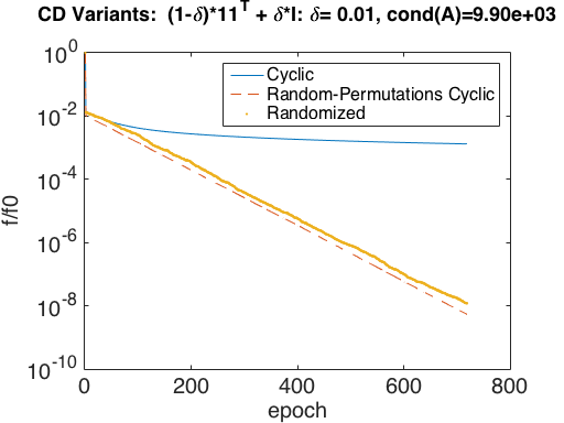
Figure 1. CCD, RPCD, and RCD on convex quadratic objective, where $A$ is defined by (1.11) with $n=100$ and $\delta=.01$.

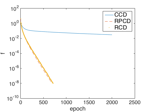
(a) Matrix (1.13).

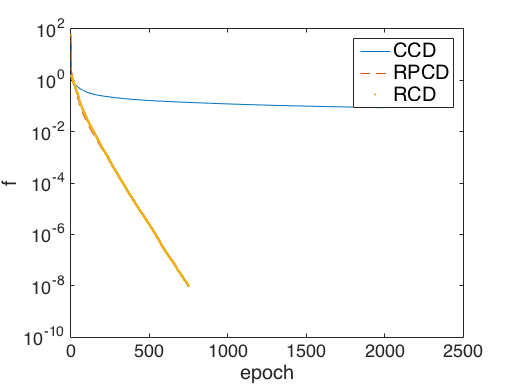
(b) Matrix (1.12) with $u$ satisfying (2.1).

Figure 2. Comparison between CCD, RPCD, and RCD on different matrices with $n=100$ and $(\delta,\epsilon)=(.01,.05)$.

2.2. RPCD Preliminaries

We now define some notation to be used in the remainder of the analysis: the matrix $C_{P}$ that defines the change in iterate $x$ over one epoch and the matrix $\bar{A}_{\epsilon}^{(\ell)}$ that defines the value $f(x^{\ell n})$ of the objective after $\ell$ epochs.

Applying to (1.13) the decomposition (1.4) into triangular and diagonal matrices, we obtain

$$P^{T}A_{\epsilon}P =(1-\delta)E+P^{T}(\delta I+\epsilon D)P+(1-\delta)E^{T}$$

(2.5) $$=(1-\delta)E+(\delta I+\epsilon D_{P})+(1-\delta)E^{T},$$

where

(2.6) $$D_{P}:=P^{T}DP,\quad E:=\left[\begin{matrix}0&0&0&\dotsc&0&0\\ 1&0&0&\dotsc&0&0\\ 1&1&0&\dotsc&0&0\\ \vdots&\vdots&\vdots&&\vdots&\vdots\\ 1&1&1&\dotsc&1&0\end{matrix}\right].$$

Following (1.5), we have for $A_{\epsilon}$ that the epoch matrix is

(2.7) $$C_{P}:=-(1-\delta)\left[(1-\delta)E+(I+\epsilon D_{P})\right]^{-1}E^{T}.$$

Our interest is in the quantity

(2.8) $$\mathbb{E}_{P_{1},P_{2},\dotsc,P_{\ell}}\,f(x^{\ell n}),\quad\ell=1,2,\dotsc,$$

where $f(x^{\ell n})$ is defined by (1.8). Adapting notation from [3], we define the matrices $\bar{A}_{\epsilon}^{(t)}$, $t=0,1,2,\dotsc,\ell$ as follows:

$$\bar{A}_{\epsilon}^{(0)} =A_{\epsilon},$$

$$\bar{A}_{\epsilon}^{(1)} =\mathbb{E}_{P_{\ell}}\left((P_{\ell}C_{P_{\ell}}^{T}P_{\ell}^{T})A_{\epsilon}(P_{\ell}C_{P_{\ell}}P_{\ell}^{T})\right),$$

$$\vdots$$

$$\bar{A}_{\epsilon}^{(\ell)} =\mathbb{E}_{P_{1},\dotsc,P_{\ell}}\left((P_{1}C_{P_{1}}^{T}P_{1}^{T})\dotsc(P_{\ell}C_{P_{\ell}}^{T}P_{\ell}^{T})A_{\epsilon}(P_{\ell}C_{P_{\ell}}P_{\ell}^{T})\dotsc(P_{1}C_{P_{1}}P_{1}^{T})\right).$$

We have the following recursive relationship between successive terms in the sequence $\bar{A}_{\epsilon}^{(t)}$, $t=0,1,2,\dotsc$:

(2.9) $$\bar{A}_{\epsilon}^{(t)} =\mathbb{E}_{P_{\ell-t+1}}(P_{\ell-t+1}C_{P_{\ell-t+1}}^{T}P_{\ell-t+1}^{T}\bar{A}_{\epsilon}^{(t-1)}P_{\ell-t+1}C_{P_{\ell-t+1}}P_{\ell-t+1}^{T})$$

$$=\mathbb{E}_{P}(PC_{P}^{T}P^{T}\bar{A}_{\epsilon}^{(t-1)}PC_{P}P^{T}),$$

where we have dropped the subscript on $P_{\ell-t+1}$ in the second equality, since the permutation matrices for each epoch are i.i.d. Using this matrix, we can compute (2.8) by

(2.10) $$\mathbb{E}_{P_{1},P_{2},\dotsc,P_{\ell}}\,f(x^{\ell n})=\frac{1}{2}\left(x^{0}\right)^{T}\bar{A}_{\epsilon}^{(t)}x^{0}.$$

3. Epoch-Wise Convergence of Expected Function Value

In this section, we analyze the behavior of the sequence of matrices $\{\bar{A}_{\epsilon}^{(t)}\}$ that govern the expected value of the objective function $f$ after $t$ epochs of RPCD. By focusing on the operation (2.9) which tracks the change from one element of this sequence to the next, we show that this sequence is bounded in norm by a quantity that decreases to zero at an asymptotic rate similar to the known rate for the fully-random variant RCD.

We show that the matrix sequence $\{\bar{A}_{\epsilon}^{(t)}\}$ is dominated by another sequence of positive definite matrices $\{\hat{A}_{\epsilon}^{(t)}\}$ that can be represented as a four-term recurrence

(3.1) $$\hat{A}_{\epsilon}^{(t)}=\hat{\eta}_{t}I+\hat{\nu}_{t}\mathbf{1}\mathbf{1}^{T}+\hat{\epsilon}_{t}D+\hat{\tau}_{t}(\mathbf{1}\mathbf{r_{1}}^{T}+\mathbf{r_{1}}\mathbf{1}^{T}),$$

where $\mathbf{r_{1}}$ is a vector such that $\|\mathbf{r_{1}}\|\leq 1$ (as defined in Section 1.4) and $(\hat{\eta}_{t},\hat{\nu}_{t},\hat{\epsilon}_{t},\hat{\tau}_{t})$ is a quadruplet of scalar coefficients for all $t=0,1,2,\cdots$. (Note that the quantities $\mathbf{r_{1}}$ in the final term are generally different for each $t$.) We set $\hat{A}_{\epsilon}^{(0)}=\bar{A}_{\epsilon}^{(0)}=A_{\epsilon}$, with

(3.2) $$\hat{\eta}_{0}=\delta,\quad\hat{\nu}_{0}=1-\delta,\quad\hat{\epsilon}_{0}=\epsilon,\quad\hat{\tau}_{0}=0,$$

and define the sequence $\{\hat{A}_{\epsilon}^{(t)}\}$ so that successive elements satisfy the same relationship as shown in (2.9) for $\{\bar{A}_{\epsilon}^{(t)}\}$, namely

$$\hat{A}_{\epsilon}^{(t+1)}\succeq\mathbb{E}_{P}(PC_{P}^{T}P^{T}\hat{A}_{\epsilon}^{(t)}PC_{P}P^{T}).$$

Our analysis consists chiefly of analyzing the convergence to zero of the sequence of quadruplets $\{(\hat{\eta}_{t},\hat{\nu}_{t},\hat{\epsilon}_{t},\hat{\tau}_{t})\}_{t=0,1,2\dotsc}$ corresponding to $\{\hat{A}_{\epsilon}^{(t)}\}_{1,2,\dotsc}$.

After several definitions and technical results in Section 3.1, we derive in Section 3.2 a tractable representation of the matrix $C_{P}$ from (1.5) that defines the transition between successive elements of the sequences $\{\bar{A}_{\epsilon}^{(t)}\}$ and $\{\hat{A}_{\epsilon}^{(t)}\}$. In Section 3.3, we examine the effect of the operation of $C_{P}$ on each of the four terms in the bounding sequence (3.1). In Section 3.4, we define the recurrence that relates successive elements of the sequence $\{(\hat{\eta}_{t},\hat{\nu}_{t},\hat{\epsilon}_{t},\hat{\tau}_{t})\}_{t=0,1,2\dotsc}$, and examine the rate at which this sequence converges to $0$. We show that the per-epoch rate is bounded by a scalar sequence that converges at a nearly linear rate of $1-1.4\delta$. (Our analysis is conservative; the true rate, observed in experiments, is often closer to $1-2\delta$.)

In most of this section, we consider the regime for parameters $n$, $\epsilon$, and $\delta$ defined by (1.14). The inequality $\delta\leq\epsilon$ is made mostly for convenience; it implies that we can replace $\delta$ by $\epsilon$ in remainder terms, and it allows wide divergence in the diagonal elements of the matrix (1.13). (We expect that the main convergence results will continue to apply in a regime in which $0\leq\epsilon<\delta$, which indeed is closer to the matrix (1.11) studied in [3], which has constant diagonals, but the remainder terms in the analysis will need to be handled differently.) In the analysis of Section 3.4, we make additional assumptions on $n$, $\epsilon$, and $\delta$.

3.1. Definitions and Technical Results

We start by defining some useful quantities, drawing on [3], and proving several elementary results. While technical, these results give an idea of the effects of applying expectations over permutations to matrices that arise in the subsequent analysis.

From (1.13) and (3.3), we have

(3.3) $$d=D\mathbf{1},\quad d_{\textrm{av}}:=\mathbf{1}^{T}d/n,\quad d_{\textrm{av,2}}:=\frac{1}{n}\mathbf{1}^{T}D^{2}\mathbf{1}.$$

From the definition of $D$ in (1.13), we have $d_{\textrm{av}}\in(0,1)$ and $d_{\textrm{av,2}}\in(0,1)$. We use $\pi$ to denote the permutation of $\{1,2,\dotsc,n\}$ associated with the permutation matrix $P$, so that for any vector $u\in\mathbb{R}^{n}$, we have

(3.4) $$P^{T}u=\left[\begin{matrix}u_{\pi(1)}\\ u_{\pi(2)}\\ \vdots\\ u_{\pi(n)}\end{matrix}\right],\quad D_{P}=P^{T}DP=\operatorname{diag}(d_{\pi(1)},d_{\pi(2)},\dotsc,d_{\pi(n)}).$$

We can see immediately that

(3.5a) $$P\mathbf{1} =\mathbf{1},$$

(3.5b) $$\mathbb{E}_{P}\,Pe_{j} =\frac{1}{n}\mathbf{1},\quad\mbox{for any $j=1,2,\dotsc,n$.}$$

A useful conditional probability is as follows:

(3.6) $$\mathbb{E}_{P\,|\,P_{i1}=1}Pe_{2}=\frac{1}{n-1}(1-e_{i}).$$

This claim follows because $Pe_{2}$ contains $n-1$ zeros and a single $1$, and the $1$ cannot appear in position $i$ (because $Pe_{1}=e_{i}$) but may appear in any other position with equal likelihood.

A quantity that appears frequently in the analysis is the matrix $F$ defined by

(3.7) $$F:=\left[\begin{matrix}0&1&0&0&\dotsc&0&0\\ 0&0&1&0&\dotsc&0&0\\ \vdots&\vdots&\vdots&&\vdots&\vdots\\ 0&0&0&0&\dotsc&0&1\\ 0&0&0&0&\dotsc&0&0\end{matrix}\right],$$

that is, the $n\times n$ matrix of all zeros except for $1$ on the diagonal immediately above the main diagonal. We see immediately that $\|F\|=1$. Several identities follow:

(3.8) $$F^{T}e_{1}=e_{2},\quad Fe_{1}=0,\quad F\mathbf{1}=\mathbf{1}-e_{n}.$$

We also have

(3.9) $$\mathbb{E}_{P}\,(PFP^{T})=\frac{1}{n}(\mathbf{1}\mathbf{1}^{T}-I).$$

To verify this claim, note that the diagonals of $PFP^{T}$ are zero for all permutation matrices $P$, while the off-diagonals are $1$ with equal probability. Thus the expected value of the $n(n-1)$ off-diagonal elements is obtained by distributing the $n-1$ nonzeros in $F$ with equal weight among all off-diagonal elements, giving an expected value of $1/n$ for each of these elements, as in (3.9).

We have the following results about quantities involving $F$.

Lemma 3.1.

(3.10a) $$PFP^{T}DPe_{1} =0,$$

(3.10b) $$\mathbb{E}_{P}\,(PF^{T}P^{T}DPe_{1}) =\frac{1}{n-1}\left[d_{\textrm{av}}\mathbf{1}-\frac{1}{n}d\right].$$

Proof.

For (3.10a), we see that $P^{T}DPe_{1}$ is a multiple of $e_{1}$, and that $Fe_{1}=0$.

For (3.10b), we use $\mathbb{E}_{i}$ to denote the expectation with respect to index $i$ uniformly distributed over $\{1,2,\dotsc,n\}$, and recall that $\pi$ denotes the permutation corresponding to $P$. We have

$$\mathbb{E}_{P}\,(PF^{T}P^{T}DPe_{1}) =\mathbb{E}_{P}\,d_{\pi(1)}PF^{T}e_{1}\quad\quad\quad$$ from (3.4)

$$=\mathbb{E}_{P}\,d_{\pi(1)}Pe_{2}$$ from (3.8)

$$=\mathbb{E}_{i}\,d_{i}\mathbb{E}_{P\,|\,P_{i1}=1}\,Pe_{2}$$

$$=\mathbb{E}_{i}\,d_{i}\frac{1}{n-1}(\mathbf{1}-e_{i})$$ from (3.6)

$$=\frac{1}{n-1}\left[d_{\textrm{av}}\mathbf{1}-\frac{1}{n}d\right],$$

as required. ∎

Finally, we make frequent use of the following trivial result about the norm of rank-1 matrices: for any vectors $v,w\in\mathbb{R}^{n}$, we have

(3.11) $$\|vw^{T}\|=\|v\|\|w\|.$$

In particular, we have from $\|\mathbf{1}\|=n^{1/2}$ that

(3.12) $$\|\mathbf{1}v^{T}\|=n^{1/2}\|v\|,$$

and in particular, using the notation of Section 1.4, we have

(3.13) $$\|\mathbf{1}\mathbf{r_{1}}^{T}\|\leq n^{1/2}.$$

3.2. Properties of the Epoch Matrix $C_{P}$

As in [3], we define

(3.14) $$\bar{L}:=-(I+(1-\delta)E)^{-1}.$$

We noted in [3] that

$$\bar{L}_{ij}=\begin{cases}-1&\;\;\mbox{if $i=j$}\\ (1-\delta)\delta^{i-j-1}&\;\;\mbox{if $i>j$}\\ 0&\;\;\mbox{if $i<j$,}\end{cases}$$

so by using notation (3.7), we have

(3.15) $$\bar{L}=-I+F^{T}+\delta\mathbf{R_{1}}.$$

We have further from a standard matrix-norm inequality together with the facts that $\|\bar{L}\|_{1}\leq 2$ and $\|\bar{L}\|_{\infty}\leq 2$ that

(3.16) $$\|\bar{L}\|\leq\sqrt{\|\bar{L}\|_{1}\|\bar{L}\|_{\infty}}\leq 2.$$

Moreover, from [3, Section 2.2], we have

$$(\bar{L}E^{T})_{ij}=\begin{cases}-\delta^{i-1}&\;\;\mbox{for $i<j$}\\ \delta^{i-j}-\delta^{i-1}&\;\;\mbox{for $i\geq j$},\end{cases}$$

so that

(3.17) $$\bar{L}E^{T}=I-e_{1}\mathbf{1}^{T}+\delta F^{T}-\delta e_{2}\mathbf{1}^{T}+\rho_{1}\delta^{2}(\mathbf{R_{1}}+\mathbf{r_{1}}\mathbf{1}^{T}).$$

(The validity of the remainder term in this expression follows from the fact that the coefficients of $\delta^{2},\delta^{3},\dotsc,\delta^{n-1}$ in $\bar{L}E^{T}$ all have the form $\mathbf{R_{1}}+\mathbf{r_{1}}\mathbf{1}^{T}$, so we can absorb them all into a single term of order $\delta^{2}$ by summation.)

The following lemma provides a useful estimate of the epoch matrix $C_{P}$.

Lemma 3.2.

Suppose that (1.14) holds. Then for $C_{P}$ defined by (1.5) and (2.7), we have

(3.18) $$(1-\delta)^{-1}C_{P} =I-e_{1}\mathbf{1}^{T}+\epsilon(-D_{P}+F^{T}D_{P})(I-e_{1}\mathbf{1}^{T})$$

$$\qquad+\delta(F^{T}-e_{2}\mathbf{1}^{T})+\epsilon^{2}(\rho_{1}\mathbf{r_{1}}\mathbf{1}^{T}+\rho_{1}\mathbf{R_{1}}).$$

Proof.

Note first that for a matrix $Y$ with $\|Y\|\leq\rho_{1}$ and for $\epsilon$ satisfying (1.14), we have

(3.19) $$(I-\epsilon Y)^{-1}=I+\epsilon Y+\epsilon^{2}(I-\epsilon Y)^{-1}Y^{2}=I+\epsilon Y+\rho_{1}\epsilon^{2}\mathbf{R_{1}}.$$

From (2.7), using definition (3.14), we have

$$(1-\delta)^{-1}C_{P} =-\left[(I+(1-\delta)E)+\epsilon D_{P}\right]^{-1}E^{T}$$

$$=[\bar{L}^{-1}-\epsilon D_{P}]^{-1}E^{T}$$

$$=[I-\epsilon\bar{L}D_{P}]^{-1}(\bar{L}E^{T}).$$

By substituting from (3.17) and (3.19) (noting that $\|\bar{L}D_{P}\|\leq\|\bar{L}\|\leq 2$ from (3.16)), we have

$$(1-\delta)^{-1}C_{P} =\left[I+\epsilon\bar{L}D_{P}+\rho_{1}\epsilon^{2}\mathbf{R_{1}}\right]\left[I-e_{1}\mathbf{1}^{T}+\delta F^{T}-\delta e_{2}\mathbf{1}^{T}+\delta^{2}(\rho_{1}\mathbf{R_{1}}+\rho_{1}\mathbf{r_{1}}\mathbf{1}^{T})\right]$$

$$=\left[I-e_{1}\mathbf{1}^{T}+\epsilon\bar{L}D_{P}(I-e_{1}\mathbf{1}^{T})+\delta(F^{T}-e_{2}\mathbf{1}^{T})+\epsilon^{2}(\rho_{1}\mathbf{R_{1}}+\rho_{1}\mathbf{r_{1}}\mathbf{1}^{T})\right],$$

where we used $\delta\leq\epsilon$ from (1.14) to absorb the term $\delta^{2}(\rho_{1}\mathbf{R_{1}}+\rho_{1}\mathbf{r_{1}}\mathbf{1}^{T})$. The result follows immediately when we use (3.15) to substitute for $\bar{L}$, and again use $\delta\leq\epsilon$ together with $\|D_{P}\|\leq 1$ and (1.17) to absorb the remainder terms. ∎

3.3. Single-Epoch Analysis

In this section we analyze the change in each term in the expression (3.1) over a single epoch. We examine in turn the following terms:

• the $I$ term: Lemma 3.3,

• the $D$ term: Lemma 3.4,

• the $\mathbf{1}\mathbf{1}^{T}$ and $(\mathbf{r_{1}}\mathbf{1}^{T}+\mathbf{1}\mathbf{r_{1}}^{T})$ terms: Lemma 3.5.

Proofs of these technical results appear in Appendix B.

Lemma 3.3.

Suppose that (1.14) holds. We have

$$(1-\delta)^{-2}\mathbb{E}_{P}\,(PC_{P}^{T}C_{P}P^{T})$$

$$=\left[I+\left(1-\frac{2}{n}\right)\mathbf{1}\mathbf{1}^{T}\right]$$

$$\;\;+\epsilon\left[-2\left(1+\frac{1}{n}\right)D+\frac{3n-2}{n(n-1)}(d\mathbf{1}^{T}+\mathbf{1}d^{T})-2\frac{n}{n-1}d_{\textrm{av}}\mathbf{1}\mathbf{1}^{T}\right]$$

$$\;\;+\delta\left(\frac{-2}{n}\right)I+\epsilon^{2}(\rho_{1}\mathbf{1}\mathbf{1}^{T}+\rho_{1}\mathbf{r_{1}}\mathbf{1}^{T}+\rho_{1}\mathbf{1}\mathbf{r_{1}}^{T}+\rho_{1}\mathbf{R_{1}})$$

$$\preceq(1+\rho_{1}\epsilon^{2})I+(1+\rho_{1}\epsilon^{2})\mathbf{1}\mathbf{1}^{T}+(\rho_{1}\epsilon n^{-1/2}+\rho_{1}\epsilon^{2})(\mathbf{1}\mathbf{r_{1}}^{T}+\mathbf{r_{1}}\mathbf{1}^{T}).$$

Lemma 3.4.

Suppose that (1.14) holds. We have

$$(1-\delta)^{-2}\mathbb{E}\,(PC_{P}^{T}P^{T}DPC_{P}P^{T})$$

$$=\left[D+d_{\textrm{av}}\mathbf{1}\mathbf{1}^{T}-\frac{1}{n}(\mathbf{1}d^{T}+d\mathbf{1}^{T})\right]+\delta\left[-\frac{2}{n}D\right]$$

$$\;\;+\epsilon\left[-2\left(1+\frac{1}{n}\right)D^{2}-\frac{d_{\textrm{av}}}{n-1}(\mathbf{1}d^{T}+d\mathbf{1}^{T})-2d_{\textrm{av,2}}\mathbf{1}\mathbf{1}^{T}\right.$$

$$\quad\quad\quad\left.+\frac{2}{n}dd^{T}+\frac{2n-1}{n(n-1)}\left(\mathbf{1}\mathbf{1}^{T}D^{2}+D^{2}\mathbf{1}\mathbf{1}^{T}\right)\right]$$

$$\;\;+\epsilon^{2}(\rho_{1}\mathbf{1}\mathbf{1}^{T}+\rho_{1}(\mathbf{r_{1}}\mathbf{1}^{T}+\mathbf{1}\mathbf{r_{1}}^{T})+\rho_{1}\mathbf{R_{1}})$$

$$\preceq D+(2\epsilon+\rho_{1}\epsilon^{2})I+(d_{\textrm{av}}+\rho_{1}\epsilon^{2})\mathbf{1}\mathbf{1}^{T}+(\rho_{1}n^{-1/2}+\rho_{1}\epsilon^{2})(\mathbf{r_{1}}\mathbf{1}^{T}+\mathbf{1}\mathbf{r_{1}}^{T}).$$

Lemma 3.5.

Suppose that (1.14) holds. For any $v\in\mathbb{R}^{n}$, we have

(3.20) $$(1-\delta)^{-2}\mathbb{E}_{P}\,(PC_{P}^{T}P^{T}(\mathbf{1}v^{T}+v\mathbf{1}^{T})PC_{P}P^{T})$$

$$=-\epsilon\left[\frac{1}{n}(dv^{T}+vd^{T})-\frac{\mathbf{1}^{T}v}{n(n-1)}(d\mathbf{1}^{T}+\mathbf{1}d^{T})+\frac{1}{n(n-1)}(Dv\mathbf{1}^{T}+\mathbf{1}v^{T}D)\right]$$

$$\;\;-\delta\left[\frac{1}{n-1}(\mathbf{1}v^{T}+v\mathbf{1}^{T})-\frac{2\mathbf{1}^{T}v}{n(n-1)}\mathbf{1}\mathbf{1}^{T}\right]$$

$$\;\;+\epsilon^{2}n^{1/2}\|v\|(\rho_{1}\mathbf{R_{1}}+\rho_{1}(\mathbf{1}\mathbf{r_{1}}^{T}+\mathbf{r_{1}}\mathbf{1}^{T})+\rho_{1}\mathbf{1}\mathbf{1}^{T})$$

so that

(3.21) $$(1-\delta)^{-2}\mathbb{E}_{P}\,(PC_{P}^{T}P^{T}(\mathbf{1}v^{T}+v\mathbf{1}^{T})PC_{P}P^{T})$$

$$\quad\quad\preceq\rho_{1}\|v\|(\epsilon n^{-1/2}+\epsilon^{2}n)I+\rho_{1}\|v\|(\epsilon n^{-3/2}+\epsilon^{2}n^{1/2})\mathbf{1}\mathbf{1}^{T}.$$

When $v=\mathbf{1}$, we have

(3.22) $$(1-\delta)^{-2}\mathbb{E}_{P}\,(PC_{P}^{T}P^{T}(\mathbf{1}\mathbf{1}^{T})PC_{P}P^{T})=\rho_{1}\epsilon^{2}\mathbf{R_{1}}\preceq\rho_{1}\epsilon^{2}I.$$

The following result summarizes Lemmas 3.3, 3.4, and 3.5, using the assumption $n\epsilon\leq 1$ from (1.14) to simplify some terms.

Theorem 3.6.

Suppose that (1.14) holds. We have

(3.23a) $$(1-\delta)^{-2}\mathbb{E}_{P}\,(PC_{P}^{T}C_{P}P^{T})$$

$$\quad\quad\preceq(1+\rho_{1}\epsilon^{2})I+(1+\rho_{1}\epsilon^{2})\mathbf{1}\mathbf{1}^{T}+\rho_{1}\epsilon n^{-1/2}(\mathbf{r_{1}}\mathbf{1}^{T}+\mathbf{1}\mathbf{r_{1}}^{T}),$$

(3.23b) $$(1-\delta)^{-2}\mathbb{E}_{P}\,(PC_{P}^{T}P^{T}\mathbf{1}\mathbf{1}^{T}PC_{P}P^{T})$$

$$\quad\quad\preceq\rho_{1}\epsilon^{2}I,$$

(3.23c) $$(1-\delta)^{-2}\mathbb{E}\,(PC_{P}^{T}P^{T}DPC_{P}P^{T})$$

$$\quad\quad\preceq D+(2\epsilon+\rho_{1}\epsilon^{2})I+(d_{\textrm{av}}+\rho_{1}\epsilon^{2})\mathbf{1}\mathbf{1}^{T}+(\rho_{1}n^{-1/2}+\rho_{1}\epsilon^{2})(\mathbf{r_{1}}\mathbf{1}^{T}+\mathbf{1}\mathbf{r_{1}}^{T})$$

(3.23d) $$(1-\delta)^{-2}\mathbb{E}_{P}\,(PC_{P}^{T}P^{T}(\mathbf{1}\mathbf{r_{1}}^{T}+\mathbf{r_{1}}\mathbf{1}^{T})PC_{P}P^{T})$$

$$\quad\quad\preceq\rho_{1}\epsilon I+\rho_{1}\epsilon n^{-1/2}\mathbf{1}\mathbf{1}^{T}.$$

Proof.

The first result (3.23a) follows immediately from Lemma 3.3 when we note that $\epsilon^{2}=n^{-1/2}(\epsilon n^{-1/2})(\epsilon n)\leq\epsilon n^{-1/2}$. The bound (3.23b) is immediate from (3.22) in Lemma 3.5. Lemma 3.4 immediately yields (3.23c). For (3.23d), we use $\epsilon n\leq 1$ and $\epsilon^{2}n^{1/2}=\epsilon(n\epsilon)n^{-1/2}\leq\epsilon n^{-1/2}$ to simplify the coefficients of $I$ and $\mathbf{1}\mathbf{1}^{T}$ in (3.21). ∎

3.4. The Four-Term Recurrence and Convergence Bound for RPCD

In this section we discuss the sequence of $n\times n$ symmetric matrices $\hat{A}_{\epsilon}^{(t)}$ that dominates the sequence $\bar{A}_{\epsilon}^{(t)}$ defined in Section 2.2. Using the results of the previous subsection, together with the four-term parametrization of $\hat{A}_{\epsilon}^{(t)}$ defined in (3.1), we derive a recurrence relationship for the sequence of quadruplets $\{(\hat{\eta}_{t},\hat{\nu}_{t},\hat{\epsilon}_{t},\hat{\tau}_{t})\}_{t=0,1,2,\dotsc}$. By finding the rate at which this sequence decreases to zero, we derive a bound on the expected values of $f$ after each epoch of RPCD.

We now show the main result for recurrence of the representation (3.1).

Theorem 3.7.

Suppose that (1.14) holds. Consider a nonnegative sequence of quadruplets $\{(\hat{\eta}_{t},\hat{\nu}_{t},\hat{\epsilon}_{t},\hat{\tau}_{t})\}_{t=0,1,2,\dotsc}$ satisfying

(3.24) $$\hat{\eta}_{0}=\delta,\quad\hat{\nu}_{0}=1-\delta,\quad\hat{\epsilon}_{0}=\epsilon,\quad\hat{\tau}_{0}=0,$$

along with the recurrence

(3.25) $$\left[\begin{matrix}\tilde{\eta}_{t+1}\\ \tilde{\nu}_{t+1}\\ \tilde{\epsilon}_{t+1}\\ \tilde{\tau}_{t+1}\end{matrix}\right]=(1-\delta)^{2}\hat{M}\left[\begin{matrix}\hat{\eta}_{t}\\ \hat{\nu}_{t}\\ \hat{\epsilon}_{t}\\ \hat{\tau}_{t}\end{matrix}\right],\quad\left[\begin{matrix}\hat{\eta}_{t+1}\\ \hat{\nu}_{t+1}\\ \hat{\epsilon}_{t+1}\\ \hat{\tau}_{t+1}\end{matrix}\right]=\left[\begin{matrix}\max(\tilde{\eta}_{t+1},0)\\ \max(\tilde{\nu}_{t+1},0)\\ \max(\tilde{\epsilon}_{t+1},0)\\ \max(\tilde{\tau}_{t+1},0)\end{matrix}\right],$$

where

(3.26) $$\hat{M}=\left[\begin{matrix}1+\rho_{1}\epsilon^{2}&\rho_{1}\epsilon^{2}&2\epsilon+\rho_{1}\epsilon^{2}&\rho_{1}\epsilon\\ 1+\rho_{1}\epsilon^{2}&0&d_{\textrm{av}}+\rho_{1}\epsilon^{2}&\rho_{1}\epsilon n^{-1/2}\\ 0&0&1&0\\ \rho_{1}\epsilon n^{-1/2}&0&\rho_{1}n^{-1/2}+\rho_{1}\epsilon^{2}&0\end{matrix}\right],$$

where each $\rho_{1}$ represents a positive quantity not much greater than $1$ and independent of $n$, $\epsilon$, and $\delta$. Then we have for $\hat{A}_{\epsilon}^{(t)}$ defined by (3.1) that $\hat{A}_{\epsilon}^{(t)}\succeq\bar{A}_{\epsilon}^{(t)}$ for all $t$.

Proof.

By definition, we have $\hat{A}_{\epsilon}^{(0)}\succeq\bar{A}_{\epsilon}^{(0)}$. Supposing that $\hat{A}_{\epsilon}^{(t)}\succeq\bar{A}_{\epsilon}^{(t)}$ for some $t\geq 0$, we have from (2.9) that

(3.27) $$\mathbb{E}_{P}(PC_{P}^{T}P^{T}\hat{A}_{\epsilon}^{(t)}PC_{P}P^{T})\succeq\mathbb{E}_{P}(PC_{P}^{T}P^{T}\bar{A}_{\epsilon}^{(t)}PC_{P}P^{T})=\bar{A}_{\epsilon}^{(t+1)}.$$

Analogous to (3.1), we define the following matrix, parametrized by the coefficients $(\tilde{\eta}_{t+1},\tilde{\nu}_{t+1},\tilde{\epsilon}_{t+1},\tilde{\tau}_{t+1})$ defined in (3.25):

(3.28) $$\tilde{A}_{\epsilon}^{(t+1)}=\tilde{\eta}_{t+1}I+\tilde{\nu}_{t+1}\mathbf{1}\mathbf{1}^{T}+\tilde{\epsilon}_{t+1}D+\tilde{\tau}_{t+1}(\mathbf{1}\mathbf{r_{1}}^{T}+\mathbf{r_{1}}\mathbf{1}^{T}).$$

Since $(\hat{\eta}_{t},\hat{\nu}_{t},\hat{\epsilon}_{t},\hat{\tau}_{t})\geq 0$, we can use Theorem 3.6 to ensure that

(3.29) $$\mathbb{E}_{P}(PC_{P}^{T}P^{T}\hat{A}_{\epsilon}^{(t)}PC_{P}P^{T})\preceq\tilde{A}_{\epsilon}^{(t+1)}.$$

A little more explanation is needed here. Because the matrices $I$, $\mathbf{1}\mathbf{1}^{T}$, and $D$ (the coefficients of $\hat{\eta}_{t}$, $\hat{\nu}_{t}$, and $\hat{\epsilon}_{t}$, respectively) are positive semidefinite, we can use the upper bounds in (3.23a), (3.23b), and (3.23c) to derive the $\preceq$ relationship. The coefficient of $\hat{\tau}_{t}$ may not be positive definite, but since $\hat{\tau}_{t}\geq 0$, we can still use the bound (3.23d) to establish the $\preceq$ relationship. Moreover, we can assume that $\tilde{\tau}_{t+1}\geq 0$, by replacing $\mathbf{r_{1}}$ by $-\mathbf{r_{1}}$ in the representation (3.28) if necessary. Thus, from (3.25), we have

$$\tilde{A}_{\epsilon}^{(t+1)}-\hat{A}_{\epsilon}^{(t+1)}=\min(\tilde{\eta}_{t+1},0)I+\min(\tilde{\nu}_{t+1},0)\mathbf{1}\mathbf{1}^{T}+\min(\tilde{\epsilon}_{t+1},0)D\preceq 0.$$

By combining this expression with (3.27) and (3.29), we obtain $\bar{A}_{\epsilon}^{(t+1)}\preceq\hat{A}_{\epsilon}^{(t+1)}$, as required. ∎

We now analyze the decay of the sequence of quadruplets $(\hat{\eta}_{t},\hat{\nu}_{t},\hat{\epsilon}_{t},\hat{\tau}_{t})$ generated by this recursion. For purposes of this analysis, we assume that all quantities $\rho_{1}$ that appear in the matrix $\hat{M}$ defined by (3.26) are bounded in magnitude by constant $\bar{\rho}$. From this constant, we define

(3.30) $$\hat{\rho}:=3.05+2.1\bar{\rho}+.6\bar{\rho}^{2}+.01\bar{\rho}^{3}.$$

We place further restrictions on the allowable regime for values of $n$, $\epsilon$, and $\delta$, in addition to those in (1.14). Specifically, we require

(3.31) $$\hat{\rho}\epsilon^{2}\leq\frac{1}{2}\delta,\quad n\geq 5.$$

As immediate consequences of these bounds, in combination with (1.14) and (3.30), we have

(3.32a) $$\hat{\rho}\epsilon\leq\frac{1}{2}\frac{\delta}{\epsilon}\leq\frac{1}{2},$$

(3.32b) $$\epsilon\leq\frac{1}{n}\leq.2\Rightarrow\delta\leq\epsilon\leq.2$$

(3.32c) $$n^{-1/2}\leq.5,\quad n^{-3/2}\leq.1,\quad n^{-2}\leq.04,$$

(3.32d) $$\bar{\rho}\epsilon^{2}\leq\frac{1}{2}\hat{\rho}\epsilon^{2}\leq\frac{1}{4}\delta\leq.05,$$

(3.32e) $$\epsilon^{2}=\frac{(n\epsilon)^{2}}{n^{2}}\leq\frac{1}{n^{2}}\leq.04.$$

Other useful consequences of (1.14) and (3.31), used repeatedly below, are as follows

(3.33a) $$(1-\delta)^{2}(1+\hat{\rho}\epsilon^{2}) \leq(1-\delta)^{2}(1+\tfrac{1}{2}\delta) \leq(1-1.4\delta),$$

(3.33b) $$(1-\delta)^{2} =(1-2\delta+\delta^{2})\leq(1-2\delta+\delta/n) \leq(1-1.8\delta).$$

We now define two sequences that can be used to bound in norm the quadruplets $(\hat{\eta}_{t},\hat{\nu}_{t},\hat{\epsilon}_{t},\hat{\tau}_{t})$. These are

(3.34a) $$\bar{\eta}_{t} :=1.5\hat{\rho}(1-1.4\delta)^{t}t\delta,$$

(3.34b) $$\bar{\epsilon}_{t} :=(1-1.8\delta)^{t}\epsilon.$$

We note immediately by combining with (3.33a) and (3.33b) that

(3.35a) $$\bar{\eta}_{t-1}\leq\frac{\bar{\eta}_{t}}{(1-1.4\delta)} \Rightarrow(1-\delta)^{2}\bar{\eta}_{t-1}\leq\bar{\eta}_{t},$$

(3.35b) $$\bar{\epsilon}_{t-1}=\frac{\bar{\epsilon}_{t}}{(1-1.8\delta)} \Rightarrow(1-\delta)^{2}\bar{\epsilon}_{t-1}\leq\bar{\epsilon}_{t}.$$

The following lemma details how the sequence of quadruplets $(\hat{\eta}_{t},\hat{\nu}_{t},\hat{\epsilon}_{t},\hat{\tau}_{t})$ is bounded in terms of the quantities in (3.35). Its proof appears in Appendix C.

Lemma 3.8.

Assume that the conditions (1.14) and (3.31) hold, and let $(\hat{\eta}_{t},\hat{\nu}_{t},\hat{\epsilon}_{t},\hat{\tau}_{t})$ be defined as in Theorem 3.7, and $\bar{\eta}_{t}$ and $\bar{\epsilon}_{t}$ be defined as in (3.34). Then the following bounds hold for all $t=1,2,\dotsc$:

(3.36a) $$0\leq\hat{\eta}_{t} \leq\bar{\eta}_{t},$$

(3.36b) $$0\leq\hat{\epsilon}_{t} \leq\bar{\epsilon}_{t},$$

(3.36c) $$0\leq\hat{\tau}_{t} \leq.5\epsilon\bar{\rho}\bar{\eta}_{t}+.54\bar{\rho}\bar{\epsilon}_{t}$$

(3.36d) $$\leq.1\bar{\rho}\bar{\eta}_{t}+.54\bar{\rho}\bar{\epsilon}_{t},$$

(3.36e) $$0\leq\hat{\nu}_{t} \leq(1.1+.01\bar{\rho}^{2})\bar{\eta}_{t}+(1.1+.1\bar{\rho}^{2})\bar{\epsilon}_{t}.$$

We are now ready to prove the main convergence result.

Theorem 3.9.

Suppose that the RPCD version of Algorithm 1 is applied to function $f$ defined by (1.3) with coefficient matrix satisfying (1.13). Suppose that the quantities $\rho_{1}$ in each recurrence matrix $\hat{M}$ in (3.25) are all bounded in magnitude by $\bar{\rho}$, and that conditions (1.14) and (3.31) hold. Then there is a constant $C$ such that for all $t=1,2,\dotsc$, we have

$$\mathbb{E}_{P_{1},P_{2},\dotsc,P_{t}}\,f(x^{tn})\leq C(1-1.4\delta)^{t}t\epsilon\|x^{0}\|^{2}.$$

indicating an asymptotic per-epoch convergence rate approaching $1-1.4\delta$.

Proof.

The proof follows from (2.10) and (3.34) when we use Lemma 3.8, the bound $\|\hat{A}_{\epsilon}^{(t)}\|\leq\bar{C}\|(\hat{\eta}_{t},\hat{\nu}_{t},\hat{\epsilon}_{t},\hat{\tau}_{t})\|$ for some $\bar{C}>0$, and the bound

$$\|(\hat{\eta}_{t},\hat{\nu}_{t},\hat{\epsilon}_{t},\hat{\tau}_{t})\|\leq\hat{C}\max(\bar{\eta}_{t},\bar{\epsilon}_{t})\leq\hat{C}(1-1.4\delta)^{t}t\epsilon,$$

for some $\hat{C}>0$, where we used $\delta\leq\epsilon$ in the last step. The final claim follows by taking the ratio of the bound after $t+1$ and $t$ epochs, which approaches $(1-1.4\delta)$ as $t\to\infty$. ∎

3.5. Decrease in the First Iteration

A behavior of all CD variants that we observe in Figures 1-2 is that the objective value decreases dramatically in the very first iteration of the algorithm. The theorem below shows that this phenomenon can be explained for both RCD and RPCD by using an extension of the analysis in [3, Theorem 3.4]. (Similar reasoning also applies for CCD in most cases, but there is no guarantee, since adversarial examples consisting of particular choices of $x^{0}$ can be constructed.) Geometrically, the phenomenon is due to the function (1.3), (1.13) increasing rapidly along just one direction — the all-one direction $\mathbf{1}$ — and more gently in other directions. Thus an exact line search along any coordinate search direction will identify a point near the bottom of this multidimensional “trench.”

Our result for first-iteration decrease is as follows.

Theorem 3.10.

Consider solving (1.3) with the matrix $A=A_{\epsilon}$ defined in (1.13), and $\epsilon\in(0,1)$, using CCD, RCD, or RPCD with exact line search. Then after a single iteration, we have

(3.37) $$f(x^{1})\leq\frac{1}{2}\sum_{j\neq i}(x^{0}_{j})^{2}(\delta+\epsilon d_{j})+\frac{\left(1-\delta\right)\left(\delta+\epsilon\right)}{2(1+\epsilon)}\left(\sum_{j\neq i}x^{0}_{j}\right)^{2},$$

where $i=i(0,0)$ is the coordinate chosen for updating in the first iteration. When RCD or RPCD is used, we further have that

(3.38) $$\mathbb{E}_{i}f(x^{1}) \leq\frac{\delta+\epsilon}{2n}\left(n-\frac{\delta+\epsilon}{1+\epsilon}\right)\|x^{0}\|^{2}+\frac{n-2}{n}\frac{(1-\delta)(\delta+\epsilon)}{(1+\epsilon)}\left(\mathbf{1}^{T}x^{0}\right)^{2}.$$

Proof.

Suppose that $i\in\{1,2,\dotsc,n\}$ is the component chosen for updating in the first iteration, which is chosen uniformly at random from $\{1,2,\dotsc,n\}$ for RPCD and RCD. After a single step of CD, we have

$$x^{1}_{i} =x^{0}_{i}-\left(x^{0}_{i}+(1-\delta)\sum_{j\neq i}\frac{x^{0}_{j}}{1+\epsilon d_{i}}\right)=-\frac{1-\delta}{1+\epsilon d_{i}}\left(\sum_{j\neq i}x^{0}_{j}\right);$$

$$x^{1}_{j} =x^{0}_{j},\;\;\mbox{for $j\neq i$.}$$

Thus, from (1.13), we have

$$f(x^{1}) =\frac{1}{2}\delta\|x^{1}\|^{2}+\frac{1}{2}(1-\delta)\left(\sum_{j=1}^{n}x^{1}_{j}\right)^{2}+\frac{1}{2}\epsilon\sum_{j=1}^{n}d_{j}(x^{1}_{j})^{2}$$

$$=\frac{1}{2}\delta\left[\sum_{j\neq i}(x^{0}_{j})^{2}+\left(\frac{1-\delta}{1+\epsilon d_{i}}\right)^{2}\left(\sum_{j\neq i}x^{0}_{j}\right)^{2}\right]$$

$$\quad\quad\quad+\frac{1}{2}(1-\delta)\left[\sum_{j\neq i}x^{0}_{j}-\frac{1-\delta}{1+\epsilon d_{i}}\sum_{j\neq i}x^{0}_{j}\right]^{2}$$

$$\quad\quad\quad+\frac{1}{2}\epsilon\left[\sum_{j\neq i}(x_{j}^{0})^{2}d_{j}+\left(\frac{1-\delta}{1+\epsilon d_{i}}\right)^{2}d_{i}\left(\sum_{j\neq i}x_{j}^{0}\right)^{2}\right]$$

(3.39) $$=\frac{1}{2}\delta\sum_{j\neq i}(x^{0}_{j})^{2}+\frac{1}{2}\epsilon\sum_{j\neq i}(x^{0}_{j})^{2}d_{j}$$

$$\quad\quad\quad+\frac{\left(\sum_{j\neq i}x^{0}_{j}\right)^{2}}{2(1+\epsilon d_{i})^{2}}\left[\delta\left(1-\delta\right)^{2}+(1-\delta)\left(\epsilon d_{i}+\delta\right)^{2}+\epsilon d_{i}\left(1-\delta\right)^{2}\right].$$

Since $d_{i}\in[0,1]$, $\delta\in(0,1)$, and $\epsilon\in(0,1)$, it can be shown that

$$\frac{1}{(1+\epsilon d_{i})^{2}}\leq\frac{1}{(1+\epsilon)^{2}},\quad\frac{\delta+\epsilon d_{i}}{1+\epsilon d_{i}}\leq\frac{\delta+\epsilon}{1+\epsilon},\quad\frac{d_{i}}{(1+\epsilon d_{i})^{2}}\leq\frac{1}{(1+\epsilon)^{2}}.$$

Thus by substitution into (3.39), we obtain

$$f(x^{1}) \leq\frac{1}{2}\delta\sum_{j\neq i}(x^{0}_{j})^{2}+\frac{1}{2}\epsilon\sum_{j\neq i}(x^{0}_{j})^{2}d_{j}$$

$$\quad+\frac{\left(\sum_{j\neq i}x^{0}_{j}\right)^{2}}{2(1+\epsilon)^{2}}\left[\delta(1-\delta)^{2}+(1-\delta)(\epsilon+\delta)^{2}+\epsilon\left(1-\delta\right)^{2}\right].$$

Further, by noting that

$$\delta(1-\delta)^{2}+(1-\delta)(\epsilon+\delta)^{2}+\epsilon\left(1-\delta\right)^{2} =(1-\delta)\left[(\delta+\epsilon)(1-\delta)+(\epsilon+\delta)^{2}\right]$$

$$=\left(1-\delta\right)(\delta+\epsilon)(1+\epsilon),$$

the desired result (3.37) is obtained.

The result (3.38) is then obtained by noting that $d_{i}\leq 1$ and that

$$\mathbb{E}_{i}\sum_{j\neq i}\left(x^{0}_{j}\right)^{2} =\frac{n-1}{n}\|x^{0}\|^{2},$$

$$\mathbb{E}_{i}\left(\sum_{j\neq i}x^{0}_{j}\right)^{2} =\left(1-\frac{2}{n}\right)\left(\mathbf{1}^{T}x^{0}\right)^{2}+\frac{1}{n}\|x^{0}\|^{2},$$

whose derivation can be found in the proof of [3, Theorem 3.4]. ∎

We can compare $f(x^{1})$ from this theorem with $f(x^{0})$ obtained by substituting into (1.13), which is

$$f(x^{0})=\frac{1}{2}\sum_{i=1}^{n}(x_{i}^{0})^{2}(\delta+\epsilon d_{i})+\frac{1}{2}(1-\delta)(\mathbf{1}^{T}x^{0})^{2}.$$

Note that the second term, which involves $(\mathbf{1}^{T}x^{0})^{2}$, decreases by a factor of approximately $(\delta+\epsilon)$ in the first iteration, whereas the first term, which involves $\|x^{0}\|^{2}$, does not change much from its original value, which is typically already small. For most starting points, the decrease is dramatic.

4. Analysis for CCD and RCD

The analysis for the RCD variant of coordinate descent for (1.3), (1.13) follows from the standard analysis [5]. The modulus of convexity $\mu$ is $\delta$, while the maximum coordinate-wise Lipschitz constant for the gradient $L_{\max}$ is $1+\epsilon$. The per-epoch linear rate of expected improvement in $f$ for RCD on $A_{\epsilon}$ is thus

(4.1) $$\rho_{\text{RCD}}\leq\left(1-\frac{\delta}{n(1+\epsilon)}\right)^{n}\approx 1-\delta+\delta\epsilon+O\left(\delta\epsilon^{2}\right),$$

yielding a complexity of $O(|\log\hat{\epsilon}|/(\delta(1-\epsilon)))$ iterations for reaching an $\hat{\epsilon}$-accurate objective. The (slightly tighter) complexity of RCD from [5, Section 4] improves this epoch bound by approximately a factor of $2$, to

(4.2) $$O\left(|\log\hat{\epsilon}|\frac{1+\epsilon+\delta}{2\delta}\right)\quad\mbox{iterations.}$$

That is, the per-epoch convergence rate of a bound on $\rho_{\text{RCD}}$ is approximately $1-2\delta/(1+\epsilon+\delta)$.

It is also shown in [5] that one can get an improved rate by non-uniform sampling of the coordinates when the coordinate-wise Lipschitz constants are not identical. In particular, for (1.3), (1.13), if the probability that the $i$th coordinate is sampled is proportional to the value of $(A_{\epsilon})_{ii}$, the result in [5] improves $\rho_{\text{RCD}}$ to

$$\rho_{\text{RCD}}\leq\left(1-\frac{\delta}{n(1+d_{\textrm{av}}\epsilon)}\right)^{n}\approx 1-\delta+\delta d_{\textrm{av}}\epsilon+O\left(\delta d_{\textrm{av}}^{2}\epsilon^{2}\right).$$

Since $d_{\textrm{av}}\in(0,1)$, this improvement is rather insignificant, and the rate is still worse than that of (4.2). (Whether nonuniform sampling can improve the complexity expression (4.2) is unknown.)

For CCD, we note that the iterates have the form

$$x^{\ell n}=C^{\ell}x^{0},$$

where $C=-(L+\Delta)^{-1}L^{T}$, where $A=L+\Delta+L^{T}$ is the triangular-diagonal splitting of $A$ (that is, $C=C_{I}$ from (1.4), (1.5)). Thus

$$f(x^{\ell n})=\frac{1}{2}(x^{0})^{T}(C^{\ell})^{T}AC^{\ell}x^{0},$$

and the asymptotic behavior of the sequence of function values is governed by $\|C^{\ell}\|^{2}$. By Gelfand’s formula [2], the asymptotic per-epoch decrease factor is thus approximately $\rho(C)^{2}$. Proposition 3.1 of [8] yields an upper bound on the per-epoch decrease factor. Noting that the largest eigenvalue of $A_{\epsilon}$ is bounded above by $n(1-\delta)+\delta+\epsilon$, their bound is as follows:

(4.3) $$\rho_{\text{CCD}}\leq 1-\max\left\{\frac{\delta}{n(n(1-\delta)+\delta+\epsilon)},\frac{\delta}{(n(1-\delta)+\delta+\epsilon)^{2}(2+\log n/\pi)^{2}},\frac{\delta}{n^{2}}\right\},$$

which is approximately $1-\delta/n^{2}$ for the ranges of values of $\delta$ and $\epsilon$ of interest in this paper. The implied iteration complexity guarantee is about a factor of $n^{2}$ worse than that for RCD. In our computational experiments, we compare empirical observations of CCD convergence rate with $\rho(C)^{2}$ rather than with (4.3).

Note that the upper bounds for convergence rates of RCD and CCD are worst-case guarantees. On the problem class (1.13), we show that the convergence rate of RPCD is similar to the bound for RCD, and we see in the next section that both bounds are quite tight in practice. The worst-case bounds on CCD are looser, in the sense that the computational behavior is not quite as poor as these bounds suggest. Nevertheless, comparison of the worst-case bounds correctly foreshadows that relative behavior of the different variants on these problems, seen in Figure 2: CCD is much slower than RCD or RPCD on this class of problems.

5. Computational Results

We report here on some experiments with variants of CD on problems of the form (1.3), (1.13). Fixing $n=100$, we tried different settings of $\epsilon$ and $\delta$, and ran the three variants CCD, RCD, and RPCD for many epochs. Results are reported in Tables 1 and 2. We obtain empirical estimates of the per-epoch asymptotic convergence rate by geometrically averaging the rate over the last 10 epochs, tabulating these observations as $\rho_{\text{CCD}}(\delta,\text{observed})$, $\rho_{\text{RCD}}(\delta,\text{observed})$, and $\rho_{\text{RPCD}}(\delta,\text{observed})$. Since we report the difference between these quantities and $1$ in the tables, larger numbers correspond to faster rates. (The numbers in the table are reported in scientific notation, with $a(b)$ representing $a\times 10^{b}$.) As noted in Section 4, we use $\rho(C)^{2}$ as the theoretical bound on the convergence rate for CCD, while we use $\rho_{\text{RCD}}$ from [5, Section 4] (which corresponds to the complexity (4.2)) as the theoretical estimate of the convergence rate for RCD. For RPCD, we used $2\delta$ as a “benchmark” value, corresponding to a per-epoch rate of $1-2\delta$, slightly faster than the $1-1.4\delta$ rate proved in Section 3.

Not all the settings of parameters $n$, $\epsilon$, and $\delta$ in these tables satisfy the conditions (1.14), (3.31) that were assumed in our analysis. We mark with an asterisk those entries for which these conditions are not satisfied. We note that the benchmark rate of $1-2\delta$ continues to hold in regimes beyond the reach of our theory. This accords with the observation that the matrix $\hat{M}$ defined in (3.26) indeed has norm very close to $1$, so that behavior of the sequence is governed chiefly by the $(1-\delta)^{2}$ factor in the recurrence (3.25).

These tables confirm that the empirical performance of RCD and RPCD is quite similar, across a wide range of parameter values, and markedly faster than CCD.

$\delta$	1.0000 (-03)	3.0000 (-03)	1.0000 (-02)	3.0000 (-02)	1.0000 (-01)
$1-\rho_{\text{CCD}}(\delta,\text{observed})$	3.4122 (-04)	3.3170 (-04)	3.3527 (-04)	6.1266 (-04)	8.1036 (-04)
$1-\rho(C)^{2}$	5.9018 (-06)	1.7170 (-05)	6.0912 (-05)	1.9453 (-04)	7.5546 (-04)
$1-\rho_{\text{RCD}}(\delta,\text{observed})$	2.6814 (-03)	5.8265 (-03)	2.1983 (-02)	6.8824 (-02)	1.4427 (-01)
$1-\rho_{\text{RCD}}(\delta,\text{predicted})$	1.9940 (-03)	5.9466 (-03)	1.9419 (-02)	5.5047 (-02)	1.5364 (-01)
$1-\rho_{\text{RPCD}}(\delta,\text{observed})$	2.7048 (-03)	6.3637 (-03)	2.1723 (-02)	6.9230 (-02)	2.0842 (-01)
Benchmark $2\delta$	2.0000 (-03)	6.0000 (-03)	2.0000 (-02)	6.0000 (-02)∗	2.0000 (-01)∗

Table 1. Comparison of CCD, RPCD, and RCD on the matrix (1.13) with $n=100$ and $\epsilon=\delta$.

$\delta$	1.0000 (-03)	3.0000 (-03)	1.0000 (-02)	3.0000 (-02)	1.0000 (-01)
$1-\rho_{\text{CCD}}(\delta,\text{observed})$	2.2372 (-04)	3.9800 (-04)	3.3538 (-04)	2.8511 (-04)	7.9319 (-04)
$1-\rho(C)^{2}$	2.7954 (-05)	5.0165 (-05)	9.7958 (-05)	2.3542 (-04)	7.8096 (-04)
$1-\rho_{\text{RCD}}(\delta,\text{observed})$	2.6143 (-03)	8.6962 (-03)	1.7869 (-02)	5.8402 (-02)	1.4545 (-01)
$1-\rho_{\text{RCD}}(\delta,\text{predicted})$	1.9763 (-03)	5.8634 (-03)	1.9019 (-02)	5.3824 (-02)	1.5364 (-01)
$1-\rho_{\text{RPCD}}(\delta,\text{observed})$	2.8377 (-03)	7.1350 (-03)	2.1157 (-02)	6.6712 (-02)	2.0501 (-01)
Benchmark $2\delta$	2.0000 (-03)	6.0000 (-03)∗	2.0000 (-02)∗	6.0000 (-02)∗	2.0000 (-01)∗

Table 2. Comparison of CCD, RPCD, and RCD on the matrix (1.13) with $n=100$ and $\epsilon=\sqrt{\delta/10}$.

Appendix A Invariance of Coordinate Descent under Diagonal Scaling

Coordinate descent applied to quadratics (1.3) with exact line search at each iterate is invariant under symmetric diagonal scalings of $A$. For any symmetric positive definite $A$ and nonzero diagonal $F$, define

(A.1) $$\tilde{A}=F^{-1}AF^{-1}.$$

Note that $\tilde{A}$ is symmetric positive definite. Consider the objective functions (1.3) defined with Hessians $A$ and $\tilde{A}$. For a given $x^{0}$, define $\tilde{x}^{0}=Fx^{0}$. The function values match at these points, that is,

(A.2) $$(\tilde{x}^{0})^{T}\tilde{A}\tilde{x}^{0}=(Fx^{0})^{T}\tilde{A}(Fx^{0})=(x^{0})^{T}Ax^{0}.$$

Considering the iterates generated by Algorithm 1 for the two functions, with $\alpha_{k}$ defined by exact line searches, and the same choices of coordinates $i(\ell,j)$ at each iteration. Assume that $Fx^{t}=\tilde{x}^{t}$ for $t=1,2,\dotsc,k$. Suppose that coordinate $i$ is chosen at iteration $k$, the updates are

$$x^{k+1}=x^{k}-\frac{(Ax^{t})_{i}}{A_{ii}}e_{i},\quad\tilde{x}^{k+1}=\tilde{x}^{k}-\frac{(\tilde{A}\tilde{x}^{t})_{i}}{\tilde{A}_{ii}}e_{i}.$$

By noting that

$$(\tilde{A}\tilde{x}^{t})_{i}=F_{ii}^{-1}(Ax^{t})_{i},\quad\tilde{A}_{ii}=F_{ii}^{-2}A_{ii},$$

and using the inductive hypothesis, it is easy to verify that $\tilde{x}^{k+1}=Fx^{k+1}$, as required.

Appendix B Proofs of Lemmas from Section 3.3

B.1. Proof of Lemma 3.3

Proof.

From Lemma 3.2, we have

$$(1-\delta)^{-2}PC_{P}^{T}C_{P}P^{T}$$

(B.1a) $$=P\left[(I-\mathbf{1}e_{1}^{T})+\epsilon(I-\mathbf{1}e_{1}^{T})(-D_{P}+D_{P}F)+\delta(F-\mathbf{1}e_{2}^{T})+\epsilon^{2}(\rho_{1}\mathbf{1}\mathbf{r_{1}}^{T}+\rho_{1}\mathbf{R_{1}})\right]$$

$$\quad\quad\left[(I-e_{1}\mathbf{1}^{T})+\epsilon(-D_{P}+F^{T}D_{P})(I-e_{1}\mathbf{1}^{T})+\delta(F^{T}-e_{2}\mathbf{1}^{T})+\epsilon^{2}(\rho_{1}\mathbf{r_{1}}\mathbf{1}^{T}+\rho_{1}\mathbf{R_{1}})\right]P^{T}$$

(B.1b) $$=\Big{\{}P(I-\mathbf{1}e_{1}^{T})(I-e_{1}\mathbf{1}^{T})P^{T}$$

$$\quad\quad+\delta\big{[}P(F-\mathbf{1}e_{2}^{T})(I-e_{1}\mathbf{1}^{T})P^{T}+P(I-\mathbf{1}e_{1}^{T})(F^{T}-e_{2}\mathbf{1}^{T})P^{T}\big{]}$$

$$\quad\quad+\epsilon P(I-\mathbf{1}e_{1}^{T})(-2D_{P}+D_{P}F+F^{T}D_{P})(I-e_{1}\mathbf{1}^{T})P^{T}\Big{\}}$$

$$\quad\quad+\epsilon^{2}(\rho_{1}(\mathbf{1}\mathbf{r_{1}}^{T}+\mathbf{r_{1}}\mathbf{1}^{T})+\rho_{1}\mathbf{1}\mathbf{1}^{T}+\rho_{1}\mathbf{R_{1}}).$$

(We give further details on the $\epsilon^{2}$ term below.) For the $O(1)$ term in (B.1b), we have from (3.5) and $e_{1}^{T}e_{1}=1$ that

(B.2) $$\mathbb{E}_{P}\,\left(P(I-\mathbf{1}e_{1}^{T})(I-e_{1}\mathbf{1}^{T})P^{T}\right)=I-\frac{2}{n}\mathbf{1}\mathbf{1}^{T}+\mathbf{1}\mathbf{1}^{T}=I+\left(1-\frac{2}{n}\right)\mathbf{1}\mathbf{1}^{T}.$$

For the first part of the $O(\delta)$ term, we have from (3.5), (3.8), (3.9), and $e_{1}^{T}e_{2}=0$ that

$$\mathbb{E}_{P}\,\left(P(F-\mathbf{1}e_{2}^{T})(I-e_{1}\mathbf{1}^{T})P^{T}\right) =\mathbb{E}_{P}\,(PFP^{T}-P\mathbf{1}e_{2}^{T}P^{T})$$

$$=\mathbb{E}_{P}\,\left(PFP^{T}-\mathbf{1}\left(\frac{1}{n}\mathbf{1}\right)^{T}\right)$$

(B.3) $$=\frac{1}{n}\mathbf{1}\mathbf{1}^{T}-\frac{1}{n}I-\frac{1}{n}\mathbf{1}\mathbf{1}^{T}=-\frac{1}{n}I.$$

(By symmetry, the second part of the $O(\delta)$ term will also have expectation $-\frac{1}{n}I$.)

For the $O(\epsilon)$ term in (B.1b), we have from (2.6), (3.8), (3.9), Lemma 3.1, and the fact that $\mathbb{E}_{P}e_{1}^{T}D_{P}e_{1}=d_{\textrm{av}}$ that

$$\mathbb{E}_{P}\,\left\{P(I-\mathbf{1}e_{1}^{T})(-2D_{P}+D_{P}F+F^{T}D_{P})(I-e_{1}\mathbf{1}^{T})P^{T}\right\}$$

$$=\mathbb{E}_{P}\,\left\{(P-\mathbf{1}e_{1}^{T})(-2P^{T}DP+P^{T}DPF+F^{T}P^{T}DP)(P^{T}-e_{1}\mathbf{1}^{T})\right\}$$

$$=-2D+\mathbb{E}_{P}(DPFP^{T}+PF^{T}P^{T}D)$$

$$\quad\quad-\mathbb{E}_{P}\left\{\mathbf{1}e_{1}^{T}(-2P^{T}D+P^{T}DPFP^{T})+(-2DP+PF^{T}P^{T}DP)e_{1}\mathbf{1}^{T}\right\}$$

$$\quad\quad+\mathbb{E}_{P}(-2e_{1}^{T}(P^{T}DP)e_{1})\mathbf{1}\mathbf{1}^{T}$$

$$=-2D+\frac{1}{n}(D(\mathbf{1}\mathbf{1}^{T}-I)+(\mathbf{1}\mathbf{1}^{T}-I)D)+\frac{2}{n}(\mathbf{1}\mathbf{1}^{T}D+D\mathbf{1}\mathbf{1}^{T})$$

$$\quad\quad-\frac{1}{n-1}\left[2d_{\textrm{av}}\mathbf{1}\mathbf{1}^{T}-\frac{1}{n}\mathbf{1}\mathbf{1}^{T}D-\frac{1}{n}D\mathbf{1}\mathbf{1}^{T}\right]-2d_{\textrm{av}}\mathbf{1}\mathbf{1}^{T}$$

$$=-2\left(1+\frac{1}{n}\right)D+\left(\frac{3}{n}+\frac{1}{n(n-1)}\right)\left(d\mathbf{1}^{T}+\mathbf{1}d^{T}\right)-2\left(1+\frac{1}{n-1}\right)d_{\textrm{av}}\mathbf{1}\mathbf{1}^{T}.$$

The lower-order terms in the main result follows by substituting this estimate along with (B.2) and (B.3) into (B.1b).

We now address the $\epsilon^{2}$ term in (B.1b). Gathering together all terms with coefficients $\epsilon^{2}$, $\epsilon\delta$, and $\delta^{2}$ from (B.1a), we have

$$\epsilon^{2}P(\rho_{1}\mathbf{1}\mathbf{r_{1}}^{T}+\rho_{1}\mathbf{R_{1}}_{(}I-e_{1}\mathbf{1}^{T})P^{T}+\mbox{(transpose)}$$

$$+\epsilon^{2}P(I-\mathbf{1}e_{1}^{T})(-D_{P})(I-F)(I-F^{T})(-D_{P})(I-e_{1}\mathbf{1}^{T})P^{T}$$

$$+\epsilon\delta P(I-\mathbf{1}e_{1}^{T})(-D_{P})(I-F)(F^{T}-e_{2}\mathbf{1}^{T})P^{T}+\mbox{(transpose)}$$

$$+\delta^{2}P(F-\mathbf{1}e_{2}^{T})(F^{T}-e_{2}\mathbf{1}^{T})P^{T}.$$

The first term in this expression (and its transpose) is clearly accounted for by the $\epsilon^{2}$ term in (B.1b). For the other $\epsilon^{2}$ term, and also the $\epsilon\delta$ terms, we use the facts that $\|F\|=1$ and $\|D_{P}(I-F)\|\leq\|D_{P}\|(\|I\|+\|F\|)=\rho_{1}$, along with $\delta\leq\epsilon$, to deduce that these terms too are accounted for by the $\epsilon^{2}$ term in (B.1b). From $\|F\|=1$ and $e_{2}^{T}e_{2}=1$, we can say the same too for the coefficient of $\delta^{2}$.

For the final “$\preceq$” claim in the lemma, we use the facts (1.16), $d\mathbf{1}^{T}=\rho_{1}n^{1/2}\mathbf{r_{1}}\mathbf{1}^{T}$ (from (3.11)), $d_{\textrm{av}}\in(0,1]$, and $D\succeq 0$, ∎

B.2. Proof of Lemma 3.4

Proof.

From Lemma 3.2, we have

$$(1-\delta)^{-2}PC_{P}^{T}D_{P}C_{P}P^{T}$$

(B.4a) $$=P\left[(I-\mathbf{1}e_{1}^{T})+\epsilon(I-\mathbf{1}e_{1}^{T})(-D_{P}+D_{P}F)+\delta(F-\mathbf{1}e_{2}^{T})+\epsilon^{2}(\rho_{1}\mathbf{1}\mathbf{r_{1}}^{T}+\rho_{1}\mathbf{R_{1}})\right]D_{P}$$

$$\quad\quad\left[(I-e_{1}\mathbf{1}^{T})+\epsilon(-D_{P}+F^{T}D_{P})(I-e_{1}\mathbf{1}^{T})+\delta(F^{T}-e_{2}\mathbf{1}^{T})+\epsilon^{2}(\rho_{1}\mathbf{r_{1}}\mathbf{1}^{T}+\rho_{1}\mathbf{R_{1}})\right]P^{T}$$

$$=P(I-\mathbf{1}e_{1}^{T})D_{P}(I-e_{1}\mathbf{1}^{T})P^{T}$$

$$\quad+\epsilon P(I-\mathbf{1}e_{1}^{T})D_{P}(-I+F)D_{P}(I-e_{1}\mathbf{1}^{T})P^{T}$$

$$\quad+\epsilon P(I-\mathbf{1}e_{1}^{T})D_{P}(-I+F^{T})D_{P}(I-e_{1}\mathbf{1}^{T})P^{T}$$

$$\quad+\delta P(F-\mathbf{1}e_{2}^{T})D_{P}(I-e_{1}\mathbf{1}^{T})P^{T}$$

$$\quad+\delta P(I-\mathbf{1}e_{1}^{T})D_{P}(F^{T}-e_{2}\mathbf{1}^{T})P^{T}$$

$$\quad+\epsilon^{2}(\rho_{1}\mathbf{1}\mathbf{1}^{T}+\rho_{1}(\mathbf{r_{1}}\mathbf{1}^{T}+\mathbf{1}\mathbf{r_{1}}^{T})+\rho_{1}\mathbf{R_{1}})$$

(B.4b) $$=P(I-\mathbf{1}e_{1}^{T})D_{P}(I-e_{1}\mathbf{1}^{T})P^{T}$$

$$\quad+\epsilon P(I-\mathbf{1}e_{1}^{T})D_{P}(-2I+F+F^{T})D_{P}(I-e_{1}\mathbf{1}^{T})P^{T}$$

$$\quad+\delta P(FD_{P}-\mathbf{1}e_{2}^{T}D_{P}+D_{P}F^{T}-D_{P}e_{2}\mathbf{1}^{T})P^{T}$$

$$\quad+\epsilon^{2}(\rho_{1}\mathbf{1}\mathbf{1}^{T}+\rho_{1}(\mathbf{r_{1}}\mathbf{1}^{T}+\mathbf{1}\mathbf{r_{1}}^{T})+\rho_{1}\mathbf{R_{1}}),$$

where we used (3.10a) from Lemma 3.1 along with $e_{2}^{T}D_{P}e_{1}=0$ to simplify the coefficient of $\delta$. (Further justification for the form of the $\epsilon^{2}$ term appears below.)

For the $O(1)$ term, we have that

$$P(I-\mathbf{1}e_{1}^{T})D_{P}(I-e_{1}\mathbf{1}^{T})P^{T} =(P-\mathbf{1}e_{1}^{T})D_{P}(P^{T}-e_{1}\mathbf{1}^{T})$$

$$=D-\mathbf{1}e_{1}^{T}P^{T}D-DPe_{1}\mathbf{1}^{T}+(e_{1}^{T}D_{P}e_{1})\mathbf{1}\mathbf{1}^{T}.$$

Thus from (3.5), we have by taking expectations over $P$ that

$$\mathbb{E}_{P}(P(I-\mathbf{1}e_{1}^{T})D_{P}(I-e_{1}\mathbf{1}^{T})P^{T}) =D-\frac{1}{n}\mathbf{1}\mathbf{1}^{T}D-\frac{1}{n}D\mathbf{1}\mathbf{1}^{T}+d_{\textrm{av}}\mathbf{1}\mathbf{1}^{T}$$

$$=D-\frac{1}{n}(\mathbf{1}d^{T}+d\mathbf{1}^{T})+d_{\textrm{av}}\mathbf{1}\mathbf{1}^{T},$$

as required.

For the coefficient of $\delta$, we have

$$P(FD_{P}-\mathbf{1}e_{2}^{T}D_{P}+D_{P}F^{T}-D_{P}e_{2}\mathbf{1}^{T})P^{T}$$

$$\quad=PFP^{T}D-\mathbf{1}e_{2}^{T}P^{T}D+DPF^{T}P^{T}-DPe_{2}\mathbf{1}^{T}.$$

Taking expectations with respect to $D$, we have from (3.5) and (3.9) that

$$\mathbb{E}_{P}(PFP^{T})D-\mathbf{1}\mathbb{E}_{P}(e_{2}^{T}P^{T})D+D\mathbb{E}_{P}(PF^{T}P^{T})-D\mathbb{E}_{P}(Pe_{2})\mathbf{1}^{T}$$

$$\quad=\frac{1}{n}(\mathbf{1}\mathbf{1}^{T}-I)D-\frac{1}{n}\mathbf{1}\mathbf{1}^{T}D+\frac{1}{n}D(\mathbf{1}\mathbf{1}^{T}-I)-\frac{1}{n}D\mathbf{1}\mathbf{1}^{T}$$

$$\quad=-\frac{2}{n}D.$$

For the coefficient of $\epsilon$, we have

$$P(I-\mathbf{1}e_{1}^{T})P^{T}DP(-2I+F+F^{T})P^{T}DP(I-e_{1}\mathbf{1}^{T})P^{T}$$

$$\quad=DP(-2I+F+F^{T})P^{T}D$$

$$\quad\quad-\mathbf{1}e_{1}^{T}P^{T}DP(-2I+F+F^{T})P^{T}D-DP(-2I+F+F^{T})P^{T}DPe_{1}\mathbf{1}^{T}$$

$$\quad\quad+\left[e_{1}^{T}P^{T}DP(-2I+F+F^{T})P^{T}DPe_{1}\right]\mathbf{1}\mathbf{1}^{T}$$

$$\quad=DP(-2I+F+F^{T})P^{T}D$$

$$\quad\quad-\mathbf{1}e_{1}^{T}P^{T}DP(-2I+F)P^{T}D-DP(-2I+F^{T})P^{T}DPe_{1}\mathbf{1}^{T}$$

(B.5) $$\quad\quad-2\left[e_{1}^{T}P^{T}D^{2}Pe_{1}\right]\mathbf{1}\mathbf{1}^{T},$$

where we used (3.10a) in Lemma 3.1 to eliminate terms that are multiples of $Fe_{1}=0$.

For the first term in (B.5), we have from (3.9) that

$$\mathbb{E}_{P}(DP(-2I+F+F^{T})P^{T}D)$$

$$\quad=-2D^{2}+D\mathbb{E}_{P}(PFP^{T})D+D\mathbb{E}_{P}(PF^{T}P^{T})D$$

$$\quad=-2D^{2}+\frac{2}{n}D(\mathbf{1}\mathbf{1}^{T}-I)D$$

(B.6) $$\quad=-2\left(1+\frac{1}{n}\right)D^{2}+\frac{2}{n}dd^{T}.$$

For the second term in (B.5), we have

$$-\mathbf{1}\mathbb{E}_{P}(e_{1}^{T}P^{T}DP(-2I+F)P^{T}D)$$

$$\quad=2\mathbf{1}\mathbb{E}_{P}(e_{1}^{T}P^{T})D^{2}-\mathbf{1}\mathbb{E}_{P}(e_{1}^{T}P^{T}DPFP^{T})D$$

$$\quad=\frac{2}{n}\mathbf{1}\mathbf{1}^{T}D^{2}-\frac{1}{n-1}\mathbf{1}\left(d_{\textrm{av}}\mathbf{1}^{T}-\frac{1}{n}\mathbf{1}^{T}D\right)D$$

$$\quad=\frac{2}{n}\mathbf{1}\mathbf{1}^{T}D^{2}-\frac{d_{\textrm{av}}}{n-1}\mathbf{1}d^{T}+\frac{1}{n(n-1)}\mathbf{1}\mathbf{1}^{T}D^{2}$$

(B.7) $$\quad=\frac{1}{n}\frac{2n-1}{n-1}\mathbf{1}\mathbf{1}^{T}D^{2}-\frac{d_{\textrm{av}}}{n-1}\mathbf{1}d^{T},$$

where we used (3.10b) from Lemma 3.1 and the definition of $d_{\textrm{av}}$ in (3.3). The third term in (B.5) is the transpose of this second term. For the final term in (B.5), we have

(B.8) $$-2\mathbb{E}_{P}(e_{1}^{T}P^{T}D^{2}Pe_{1})\mathbf{1}\mathbf{1}^{T}=-2d_{\textrm{av,2}}\mathbf{1}\mathbf{1}^{T}.$$

By substituting (B.6), (B.7), and (B.8) into (B.5), we obtain the required coefficient of $\epsilon$.

We return to verifying the form of the $\epsilon^{2}$ term in (B.4b). The coefficients of $\epsilon^{2}$, $\epsilon\delta$, and $\delta^{2}$ terms from (B.4a) are are follows:

$$\epsilon^{2}P(I-\mathbf{1}e_{1}^{T})D_{P}(\rho_{1}\mathbf{r_{1}}\mathbf{1}^{T}+\rho_{1}\mathbf{R_{1}})P^{T}+\mbox{(transpose)}$$

$$+\epsilon^{2}P(I-\mathbf{1}e_{1}^{T})(-D_{P})(I-F)D_{P}(I-F^{T})(-D_{P})(I-e_{1}\mathbf{1}^{T})P^{T}$$

$$+\epsilon\delta P(I-\mathbf{1}e_{1}^{T})(-D_{P})(I-F)D_{P}(F^{T}-e_{2}\mathbf{1}^{T})P^{T}+\mbox{(transpose)}$$

$$+\delta^{2}P(F-\mathbf{1}e_{2}^{T})D_{P}(F^{T}-e_{2}\mathbf{1}^{T}).$$

By making use of the bounds $\|I\|=\|F\|=1$, $\|D_{P}\|\leq 1$, $\|e_{1}\|=\|e_{2}\|=1$, and $\delta\leq\epsilon$, we see that this expression is accounted for by the coefficient of $\epsilon^{2}$ in (B.4b).

For the final “$\preceq$” relationship, we use $dd^{T}\preceq nI$ to obtain $(2/n)\epsilon dd^{T}\preceq 2\epsilon I$, $\mathbf{1}\mathbf{1}^{T}D^{2}=n^{1/2}\mathbf{1}\mathbf{r_{1}}^{T}$ to bound the terms with $\mathbf{1}\mathbf{1}^{T}D^{2}$ (and similarly for $D^{2}\mathbf{1}\mathbf{1}^{T}$), $D^{2}\succeq 0$, $\mathbf{1}d^{T}=n^{1/2}\mathbf{1}\mathbf{r_{1}}^{T}$ to obtain $-(1/n)\mathbf{1}d^{T}\preceq n^{-1/2}\mathbf{1}\mathbf{r_{1}}^{T}$, and $\mathbf{R_{1}}\preceq I$. ∎

B.3. Proof of Lemma 3.5

Proof.

We have

$$PC_{P}^{T}P^{T}(\mathbf{1}v^{T}+v\mathbf{1}^{T})PC_{P}P^{T}=PC_{P}^{T}P^{T}\mathbf{1}v^{T}PC_{P}P^{T}+\operatorname{(transpose)},$$

where we use $\operatorname{(transpose)}$ to denote the transpose of the explicitly stated terms. From Lemma 3.2 and $P^{T}\mathbf{1}=\mathbf{1}$, we have

$$(1-\delta)^{-2}PC_{P}^{T}P^{T}\mathbf{1}v^{T}PC_{P}P^{T}$$

(B.9a) $$=P\left[(I-\mathbf{1}e_{1}^{T})+\epsilon(I-\mathbf{1}e_{1}^{T})(-D_{P}+D_{P}F)+\delta(F-\mathbf{1}e_{2}^{T})+\epsilon^{2}(\rho_{1}\mathbf{1}\mathbf{r_{1}}^{T}+\rho_{1}\mathbf{R_{1}})\right]\mathbf{1}v^{T}P$$

$$\quad\quad\left[(I-e_{1}\mathbf{1}^{T})+\epsilon(-D_{P}+F^{T}D_{P})(I-e_{1}\mathbf{1}^{T})+\delta(F^{T}-e_{2}\mathbf{1}^{T})+\epsilon^{2}(\rho_{1}\mathbf{r_{1}}\mathbf{1}^{T}+\rho_{1}\mathbf{R_{1}})\right]P^{T}$$

(B.9b) $$=P(I-\mathbf{1}e_{1}^{T})\mathbf{1}v^{T}P(I-e_{1}\mathbf{1}^{T})P^{T}$$

$$\quad\quad-\epsilon\big{\{}P(I-\mathbf{1}e_{1}^{T})D_{P}(I-F)\mathbf{1}v^{T}P(I-e_{1}\mathbf{1}^{T})P^{T}$$

$$\quad\quad\quad\quad+P(I-\mathbf{1}e_{1}^{T})\mathbf{1}v^{T}P(I-F^{T})D_{P}(I-e_{1}\mathbf{1}^{T})P^{T}\big{\}}$$

$$\quad\quad+\delta\big{\{}P(F-\mathbf{1}e_{2}^{T})\mathbf{1}v^{T}P(I-e_{1}\mathbf{1}^{T})P^{T}$$

$$\quad\quad\quad\quad+P(I-\mathbf{1}e_{1}^{T})\mathbf{1}v^{T}P(F^{T}-e_{2}\mathbf{1}^{T})P^{T}\big{\}}$$

$$\quad\quad+\epsilon^{2}n^{1/2}\|v\|(\rho_{1}\mathbf{R_{1}}+\rho_{1}(\mathbf{r_{1}}\mathbf{1}^{T}+\mathbf{1}\mathbf{r_{1}}^{T})+\rho_{1}\mathbf{1}\mathbf{1}^{T}).$$

To derive the remainder term (the coefficient of $\epsilon^{2}$ in (B.9b)), we need to consider the coefficients of $\epsilon^{2}$, $\delta\epsilon$, and $\delta^{2}$ from (B.9a). The coefficient of the $\epsilon^{2}$ term is

$$\epsilon^{2}P(I-\mathbf{1}e_{1}^{T})\mathbf{1}v^{T}P(\rho_{1}\mathbf{r_{1}}\mathbf{1}^{T}+\rho_{1}\mathbf{R_{1}})P^{T}$$

$$\quad+\epsilon^{2}P(\rho_{1}\mathbf{1}\mathbf{r_{1}}^{T}+\rho_{1}\mathbf{R_{1}})\mathbf{1}v^{T}P(I-e_{1}\mathbf{1}^{T})P^{T}$$

(B.10) $$\quad+\epsilon^{2}P(I-\mathbf{1}e_{1}^{T})(-D_{P}+D_{P}F)\mathbf{1}v^{T}(-D_{P}+F^{T}D_{P})(I-e_{1}\mathbf{1}^{T})P^{T}.$$

Using $(I-\mathbf{1}e_{1}^{T})\mathbf{1}=\mathbf{1}-\mathbf{1}=0$, we see that the first term in this expression vanishes. From (3.7) and (3.8), we have several other identities:

(B.11) $$(I-F)\mathbf{1}=e_{n},\quad(F-\mathbf{1}e_{2}^{T})\mathbf{1}=F\mathbf{1}-\mathbf{1}=-e_{n}.$$

In the third term, we thus have that $(-D_{P}+D_{P}F)\mathbf{1}=-D_{P}(I-F)\mathbf{1}=-D_{P}e_{n}=\rho_{1}\mathbf{r_{1}}$. We also have that $e_{1}^{T}D_{P}e_{n}=0$ and $v^{T}(-D_{P}+F^{T}D_{P})=\rho_{1}\|v\|\mathbf{r_{1}}^{T}$. Thus (B.10) becomes

$$\epsilon^{2}P(\rho_{1}(\mathbf{r_{1}}^{T}\mathbf{1})\mathbf{1}+\rho_{1}\mathbf{R_{1}}\mathbf{1})v^{T}(I-Pe_{1}\mathbf{1}^{T})$$

$$\quad+\rho_{1}\epsilon^{2}\|v\|P(I-\mathbf{1}e_{1}^{T})(-D_{P}e_{n})\mathbf{r_{1}}^{T}(I-e_{1}\mathbf{1}^{T})P^{T}$$

$$=\epsilon^{2}(\rho_{1}n^{1/2}\mathbf{1}+\rho_{1}n^{1/2}\mathbf{r_{1}})(v^{T}-\|v\|\rho_{1}\mathbf{1}^{T})$$

$$\quad+\rho_{1}\epsilon^{2}\|v\|\mathbf{r_{1}}\mathbf{r_{1}}^{T}(I-e_{1}\mathbf{1}^{T})P^{T}$$

$$=\epsilon^{2}n^{1/2}\|v\|(\rho_{1}\mathbf{R_{1}}+\rho_{1}(\mathbf{1}\mathbf{r_{1}}^{T}+\mathbf{r_{1}}\mathbf{1}^{T})+\rho_{1}\mathbf{1}\mathbf{1}^{T}),$$

which is accounted for by the $\epsilon^{2}$ term in (B.9b). We turn next to the coefficient of $\epsilon\delta$ in (B.9a). This term consists of the following expression plus its transpose:

$$\delta\epsilon P(I-\mathbf{1}e_{1}^{T})(-D_{P})(I-F)\mathbf{1}v^{T}P(F^{T}-e_{2}\mathbf{1}^{T})P^{T}$$

$$=\delta\epsilon(P-\mathbf{1}e_{1}^{T})(-D_{P})e_{n}v^{T}P(F^{T}-e_{2}\mathbf{1}^{T})P^{T}\quad\mbox{from \eqref{eq:F1en}}$$

$$=\delta\epsilon(PD_{P}e_{n})v^{T}P(F^{T}-e_{2}\mathbf{1}^{T})P^{T}\quad\mbox{since $e_{1}^{T}D_{P}e_{n}=0$}$$

$$=\delta\epsilon\mathbf{r_{1}}(\rho_{1}\|v\|\mathbf{r_{1}}^{T}-\rho_{1}\|v\|\mathbf{1}^{T}).$$

Because $\delta\leq\epsilon$, this term (plus its transpose) can also be accounted for by the $\epsilon^{2}$ term in (B.9b). For the coefficient of $\delta^{2}$ in (B.9a), we have, using (B.11) again,

$$\delta^{2}P(F-\mathbf{1}e_{2}^{T})\mathbf{1}v^{T}P(F^{T}-e_{2}\mathbf{1}^{T})P^{T}$$

$$=-\delta^{2}Pe_{n}v^{T}P(F^{T}-e_{2}\mathbf{1}^{T})P^{T}=\delta^{2}\mathbf{r_{1}}\|v\|(\rho_{1}\mathbf{r_{1}}^{T}+\rho_{1}\mathbf{1}^{T})=\delta^{2}\|v\|(\rho_{1}\mathbf{R_{1}}+\rho_{1}\mathbf{r_{1}}\mathbf{1}^{T}),$$

which can also be absorbed into the $\epsilon^{2}$ term in (B.9b).

Returning to the lower-order terms in (B.9b), we use again the fact that $(I-\mathbf{1}e_{1}^{T})\mathbf{1}=0$ to eliminate the $O(1)$ term, and also one of the two terms in the coefficients of both $\epsilon$ and $\delta$. We thus obtain

$$(1-\delta)^{-2}PC_{P}^{T}P^{T}\mathbf{1}v^{T}PC_{P}P^{T}$$

$$=-\epsilon\big{\{}P(I-\mathbf{1}e_{1}^{T})D_{P}(I-F)\mathbf{1}v^{T}P(I-e_{1}\mathbf{1}^{T})P^{T}\big{\}}$$

$$\quad\quad+\delta\big{\{}P(F-\mathbf{1}e_{2}^{T})\mathbf{1}v^{T}P(I-e_{1}\mathbf{1}^{T})P^{T}\big{\}}$$

(B.12) $$\quad\quad+\epsilon^{2}n^{1/2}\|v\|(\rho_{1}\mathbf{R_{1}}+\rho_{1}(\mathbf{r_{1}}\mathbf{1}^{T}+\mathbf{1}\mathbf{r_{1}}^{T})+\rho_{1}\mathbf{1}\mathbf{1}^{T}).$$

Additionally, we have from (2.6) that

$$P(I-e_{1}\mathbf{1}^{T})P^{T} =I-(Pe_{1})\mathbf{1}^{T}$$

$$P(I-\mathbf{1}e_{1}^{T})D_{P} =P(I-\mathbf{1}e_{1}^{T})P^{T}DP=(I-\mathbf{1}(Pe_{1})^{T})DP.$$

By substituting these identities into (B.12), we obtain

$$(1-\delta)^{-2}PC_{P}^{T}P^{T}\mathbf{1}v^{T}PC_{P}P^{T}$$

$$=-\epsilon\big{\{}(I-\mathbf{1}(Pe_{1})^{T})DPe_{n}v^{T}(I-(Pe_{1})\mathbf{1}^{T})\big{\}}$$

$$\quad\quad-\delta\big{\{}(Pe_{n})v^{T}(I-(Pe_{1})\mathbf{1}^{T})\big{\}}$$

$$\quad\quad+\epsilon^{2}n^{1/2}\|v\|(\rho_{1}\mathbf{R_{1}}+\rho_{1}(\mathbf{1}\mathbf{r_{1}}^{T}+\mathbf{r_{1}}\mathbf{1}^{T})+\rho_{1}\mathbf{1}\mathbf{1}^{T})$$

$$=-\epsilon\big{\{}D(Pe_{n})v^{T}(I-(Pe_{1})\mathbf{1}^{T})\big{\}}-\delta\big{\{}(Pe_{n})v^{T}(I-(Pe_{1})\mathbf{1}^{T})\big{\}}$$

(B.13) $$\quad\quad+\epsilon^{2}n^{1/2}\|v\|(\rho_{1}\mathbf{R_{1}}+\rho_{1}(\mathbf{1}\mathbf{r_{1}}^{T}+\mathbf{r_{1}}\mathbf{1}^{T})+\rho_{1}\mathbf{1}\mathbf{1}^{T})$$

where the second equality follows from

$$(Pe_{1})^{T}D(Pe_{n})=e_{1}^{T}D_{P}e_{n}=0,$$

since $D_{P}$ is diagonal for all $P$.

Taking expectations, we have for the coefficient of $(-\delta)$ in (B.13) that

$$\mathbb{E}_{P}\,\big{(}(Pe_{n})v^{T}(I-(Pe_{1})\mathbf{1}^{T})\big{)} =\mathbb{E}_{P}\,(Pe_{n})v^{T}-\big{[}\mathbb{E}_{P}\,(Pe_{n})(v^{T}Pe_{1})\big{]}\mathbf{1}^{T}$$

$$=\frac{1}{n}\mathbf{1}v^{T}-\frac{1}{n(n-1)}\left(\sum_{\stackrel{{\scriptstyle i,j=1}}{{i\neq j}}}^{n}v_{i}e_{j}\right)\mathbf{1}^{T}$$

$$=\frac{1}{n}\mathbf{1}v^{T}-\frac{1}{n(n-1)}\left(\sum_{i=1}^{n}v_{i}\sum_{\stackrel{{\scriptstyle j=1}}{{i\neq j}}}^{n}e_{j}\right)\mathbf{1}^{T}$$

$$=\frac{1}{n}\mathbf{1}v^{T}-\frac{1}{n(n-1)}\left(\sum_{i=1}^{n}v_{i}(\mathbf{1}-e_{i})\right)\mathbf{1}^{T}$$

$$=\frac{1}{n}\mathbf{1}v^{T}-\frac{1}{n(n-1)}\left((\mathbf{1}^{T}v)\mathbf{1}\mathbf{1}^{T}-v\mathbf{1}^{T})\right)$$

(B.14) $$=\frac{1}{n}\mathbf{1}v^{T}-\frac{(\mathbf{1}^{T}v)}{n(n-1)}\mathbf{1}\mathbf{1}^{T}+\frac{1}{n(n-1)}v\mathbf{1}^{T},$$

where the second equality is from a conditional expectation over permutation matrices $P$ such that $Pe_{1}=j$ and $Pe_{n}=i$, for all $i,j=1,2,\dotsc,n$ with $i\neq j$. By combining (B.14) with its transpose, we obtain the full coefficient of $(-\delta)$ in (3.20), which is

$$\left(\frac{1}{n}+\frac{1}{n(n-1)}\right)(\mathbf{1}v^{T}+v\mathbf{1}^{T})-\frac{2(\mathbf{1}^{T}v)}{n(n-1)}\mathbf{1}\mathbf{1}^{T}=\frac{1}{n-1}(\mathbf{1}v^{T}+v\mathbf{1}^{T})-\frac{2(\mathbf{1}^{T}v)}{n(n-1)}\mathbf{1}\mathbf{1}^{T}.$$

This verifies the $O(\delta)$ term in (3.20).

We note that the coefficient of $(-\epsilon)$ in (B.13) is the same as the coefficient of $(-\delta)$, except for being multiplied from the left by $D$, which is independent of $P$. Thus the expectation of this term is simply (B.14), multiplied from the left by $D$, that is,

$$\frac{1}{n}D\mathbf{1}v^{T}-\frac{\mathbf{1}^{T}v}{n(n-1)}(D\mathbf{1})\mathbf{1}^{T}+\frac{1}{n(n-1)}Dv\mathbf{1}^{T}=\frac{1}{n}dv^{T}-\frac{\mathbf{1}^{T}v}{n(n-1)}d\mathbf{1}^{T}+\frac{1}{n(n-1)}Dv\mathbf{1}^{T}.$$

We obtain the full coefficient of $(-\epsilon)$ in (3.20) by adding this quantity to its transpose, to obtain

$$\frac{1}{n}(dv^{T}+vd^{T})-\frac{\mathbf{1}^{T}v}{n(n-1)}(d\mathbf{1}^{T}+\mathbf{1}d^{T})+\frac{1}{n(n-1)}(Dv\mathbf{1}^{T}+\mathbf{1}v^{T}D),$$

as required.

For the “$\preceq$” result (3.21), we use

$$\|dv^{T}\|=n^{1/2}\rho_{1}\|v\|,\quad\|d\|\leq n^{1/2},\quad|\mathbf{1}^{T}v|\leq n^{1/2}\|v\|,\quad\|Dv\|\leq\|d\|,$$

together with $\delta\leq\epsilon$ from (1.14). We also use $\mathbf{r_{1}}\mathbf{1}^{T}+\mathbf{1}\mathbf{r_{1}}^{T}=n^{1/2}\mathbf{R_{1}}$ and $-I\preceq\mathbf{R_{1}}\preceq I$ for symmetric $\mathbf{R_{1}}$ to absorb the $\epsilon^{2}(\mathbf{r_{1}}\mathbf{1}^{T}+\mathbf{1}\mathbf{r_{1}}^{T})$ term in (3.20) into the $I$ term in (3.21).

For (3.22), we have

$$(1-\delta)^{-1}PC_{P}^{T}P^{T}\mathbf{1}$$

$$=(1-\delta)^{-1}PC_{P}^{T}\mathbf{1}$$

$$=P\left[(I-\mathbf{1}e_{1}^{T})+\epsilon(I-\mathbf{1}e_{1}^{T})D_{P}(-I+F)+\delta(F-\mathbf{1}e_{2}^{T})+\epsilon^{2}(\rho_{1}\mathbf{1}\mathbf{r_{1}}^{T}+\rho_{1}\mathbf{R_{1}})\right]\mathbf{1}$$

$$=P\left[-\epsilon(I-\mathbf{1}e_{1}^{T})D_{P}e_{n}-\delta e_{n}+\epsilon^{2}n^{1/2}(\rho_{1}\mathbf{1}+\rho_{1}\mathbf{r_{1}})\right]$$

(B.15) $$=P\left[-\epsilon D_{P}e_{n}-\delta e_{n}+\epsilon^{2}n^{1/2}(\rho_{1}\mathbf{1}+\rho_{1}\mathbf{r_{1}})\right],$$

where we used the following identities for the third equality:

$$(I-\mathbf{1}e_{1}^{T})\mathbf{1}=0,\quad(-I+F)\mathbf{1}=-e_{n},\quad(F-\mathbf{1}e_{2}^{T})\mathbf{1}=-e_{n},$$

$$\mathbf{r_{1}}^{T}\mathbf{1}\leq n^{1/2},\quad\mathbf{R_{1}}\mathbf{1}=\rho_{1}n^{1/2}\mathbf{r_{1}},$$

and $e_{1}^{T}D_{P}e_{n}=0$ for the fourth equality. By substituting $D_{P}=P^{T}DP$ into (B.15), we obtain

$$(1-\delta)^{-1}PC_{P}P^{T}\mathbf{1}=-\epsilon DPe_{n}-\delta Pe_{n}+\epsilon^{2}n^{1/2}(\rho_{1}\mathbf{1}+\rho_{1}\mathbf{r_{1}}).$$

By taking the outer product of this vector with itself, and using $\delta\leq\epsilon$, we obtain

$$(1-\delta)^{-2}PC_{P}^{T}P^{T}\mathbf{1}\mathbf{1}^{T}PC_{P}P^{T}$$

$$=\epsilon^{2}D(Pe_{n})(Pe_{n})^{T}D+\delta\epsilon[D(Pe_{n})(Pe_{n})^{T}+(Pe_{n})(Pe_{n})^{T}D]+\delta^{2}(Pe_{n})(Pe_{n})^{T}$$

$$\quad\quad+\epsilon^{3}n^{1/2}(\rho_{1}(\mathbf{1}\mathbf{r_{1}}^{T}+\mathbf{r_{1}}\mathbf{1}^{T})+\rho_{1}\mathbf{R_{1}}),$$

where in the remainder term we used $\|Pe_{n}\|=1$ and $\|D\|\leq 1$. By taking expectations over $P$, and using $\mathbb{E}_{P}(Pe_{n})(Pe_{n})^{T}=n^{-1}I$, we obtain

$$(1-\delta)^{-2}\mathbb{E}_{P}(PC_{P}^{T}P^{T}\mathbf{1}\mathbf{1}^{T}PC_{P}P^{T})$$

$$=n^{-1}\epsilon^{2}D^{2}+2n^{-1}\epsilon\delta D+n^{-1}\delta^{2}I+\epsilon^{3}n^{1/2}(\rho_{1}(\mathbf{1}\mathbf{r_{1}}^{T}+\mathbf{r_{1}}\mathbf{1}^{T})+\rho_{1}\mathbf{R_{1}})$$

$$=\rho_{1}\epsilon^{2}n^{-1}\mathbf{R_{1}}+\rho_{1}\epsilon^{3}n\mathbf{R_{1}}=\rho_{1}\epsilon^{2}\mathbf{R_{1}},$$

where we used (1.14) in the last expression to deduce that $\epsilon^{3}n\leq\epsilon^{2}$.

∎

Appendix C Proof of Lemma 3.8

Proof.

Note first that $\hat{\eta}_{t}$, $\hat{\nu}_{t}$, $\hat{\epsilon}_{t}$, and $\hat{\tau}_{t}$ are all nonnegative by definition. In this proof, we use repeatedly that they can be bounded by $|\tilde{\eta}_{t}|$, $|\tilde{\nu}_{t}|$, $|\tilde{\epsilon}_{t}|$, and $|\tilde{\tau}_{t}|$, respectively, though the $|\cdot|$ are unnecessary in the case of $\tilde{\epsilon}_{t}$ (since its exact value can be determined trivially from (3.25)) and in the case of $\tilde{\tau}_{t}$ (which can be assumed without loss of generality to be nonnegative, as mentioned in the proof of Theorem 3.7).

The proof is by induction on $t$. We show first that the bounds (3.36) hold for $t=1$.

We have from (3.33b) and the obvious property $\hat{\epsilon}_{t}=(1-\delta)^{2t}\epsilon$ from (3.25) that

$$\hat{\epsilon}_{1}=(1-\delta)^{2}\epsilon\leq(1-1.8\delta)\epsilon=\bar{\epsilon}_{1},$$

verifying (3.36b) for $t=1$. For (3.36a), we have from (3.25) with $t=0$, using the initial values (3.24) and the bounds in (3.32) that that

$$(1-\delta)^{-2}\hat{\eta}_{1}\leq(1-\delta)^{-2}|\tilde{\eta}_{1}| \leq(1+\bar{\rho}\epsilon^{2})\delta+\bar{\rho}\epsilon^{2}(1-\delta)+(2\epsilon+\bar{\rho}\epsilon^{2})\epsilon$$

$$=\delta+\left(2+\bar{\rho}+\bar{\rho}\epsilon\right)\epsilon^{2}$$

$$\leq\delta+\hat{\rho}\epsilon^{2}\leq 3\delta.$$

It follows from $\hat{\rho}\geq 3$ and $\delta\leq.2$ (see (3.32b)) that

$$\hat{\eta}_{1}\leq 3(1-\delta)^{2}\delta\leq 3(1-1.4\delta)\delta\leq 1.5\hat{\rho}(1-1.4\delta)\delta=\bar{\eta}_{1},$$

verifying (3.36a) for $t=1$. For (3.36c) with $t=1$, we have

$$\hat{\tau}_{1}=\tilde{\tau}_{1} \leq(1-\delta)^{2}\bar{\rho}\epsilon n^{-1/2}\delta+(1-\delta)^{2}(\bar{\rho}n^{-1/2}+\bar{\rho}\epsilon^{2})\epsilon$$

$$\leq(1-1.4\delta)(.5)\bar{\rho}\epsilon\delta+(1-1.8\delta)(.5\bar{\rho}+.04\bar{\rho})\epsilon,$$

where for the second inequality we used $n^{-1/2}\leq.5$ and $\epsilon^{2}\leq.04$. Continuing, we use $\bar{\eta}_{1}\geq 4(1-1.4\delta)\delta$ and $\bar{\epsilon}_{1}=(1-1.8\delta)\epsilon$ to write

(C.1) $$\hat{\tau}_{1}\leq\frac{1}{8}\bar{\rho}\epsilon\bar{\eta}_{1}+.54\bar{\rho}\bar{\epsilon}_{1},$$

which suffices to prove (3.36c) for $t=1$. For (3.36d), we simply use $\epsilon\leq.2$ from (3.32).

For (3.36e) with $t=1$, we have from (3.25) and (3.24), using again $\epsilon^{2}\leq.04$ from (3.32), as well as $d_{\textrm{av}}\leq 1$ from (3.3) that

$$\hat{\nu}_{t}\leq|\tilde{\nu}_{t}| \leq(1-\delta)^{2}(1+\bar{\rho}\epsilon^{2})\delta+(1-\delta)^{2}(d_{\textrm{av}}+\bar{\rho}\epsilon^{2})\epsilon$$

$$\leq(1-\delta)^{2}(1+\bar{\rho}\epsilon^{2})\delta+(1-\delta)^{2}(1+.04\bar{\rho})\epsilon$$

$$\leq(1-1.4\delta)\hat{\rho}\delta+(1-1.8\delta)(1+.04\bar{\rho})\epsilon$$

$$\leq\bar{\eta}_{1}+(1+.04\bar{\rho})\bar{\epsilon}_{1},$$

which suffices to demonstrate (3.36e) for $t=1$.

Assuming now that (3.36) holds for some $t\geq 1$, we prove that the bounds holds for $t+1$ as well. We start with (3.36c). It follows from (3.25) that

$$(1-\delta)^{-2}\hat{\tau}_{t+1}\leq(1-\delta)^{-2}|\tilde{\tau}_{t+1}| \leq\bar{\rho}\epsilon n^{-1/2}|\hat{\eta}_{t}|+(\bar{\rho}n^{-1/2}+\bar{\rho}\epsilon^{2})|\hat{\epsilon}_{t}|$$

$$\leq.5\bar{\rho}\epsilon\bar{\eta}_{t}+(.5\bar{\rho}+.04\bar{\rho})\bar{\epsilon}_{t}$$

$$\leq.5\bar{\rho}\epsilon\bar{\eta}_{t}+.54\bar{\rho}\bar{\epsilon}_{t}.$$

It then follows from (3.35) that

$$\hat{\tau}_{t+1}\leq.5\bar{\rho}\epsilon\bar{\eta}_{t+1}+.54\bar{\rho}\bar{\epsilon}_{t+1},$$

as required. As earlier, (3.36d) follows immediately when we note that $\epsilon\leq.2$, from (3.32).

For (3.36e), we have

$$(1-\delta)^{-2}\hat{\nu}_{t+1} \leq(1+\bar{\rho}\epsilon^{2})\bar{\eta}_{t}+(d_{\textrm{av}}+\bar{\rho}\epsilon^{2})\bar{\epsilon}_{t}+\bar{\rho}\epsilon n^{-1/2}|\hat{\tau}_{t}|$$

$$\leq(1+\bar{\rho}\epsilon^{2}+(\bar{\rho}\epsilon n^{-1/2})(.1)\bar{\rho})\bar{\eta}_{t}+(d_{\textrm{av}}+\bar{\rho}\epsilon^{2}+(\bar{\rho}\epsilon n^{-1/2})(.54)\bar{\rho})\bar{\epsilon}_{t},$$

where we used (3.36d) for the second inequality. Using now the bounds $\bar{\rho}\epsilon^{2}\leq.05$ and $n^{-1/2}\leq.5$ (from (3.32)), $d_{\textrm{av}}\leq 1$, and $\epsilon n^{-1/2}=(\epsilon n)n^{-3/2}\leq n^{-3/2}\leq.1$, we have

$$(1-\delta)^{-2}\hat{\nu}_{t+1}\leq(1.1+.01\bar{\rho}^{2})\bar{\eta}_{t}+(1.1+.1\bar{\rho}^{2})\bar{\epsilon}_{t},$$

so that

$$\hat{\nu}_{t+1}\leq(1.1+.01\bar{\rho}^{2})\bar{\eta}_{t+1}+(1.1+.1\bar{\rho}^{2})\bar{\epsilon}_{t+1},$$

as required.

The proof for (3.36b) is trivial, since

$$\hat{\epsilon}_{t+1}=(1-\delta)^{2(t+1)}\epsilon=(1-\delta)^{2}\hat{\epsilon}_{t}\leq(1-1.8\delta)\hat{\epsilon}_{t}\leq(1-1.8\delta)\bar{\epsilon}_{t}=\bar{\epsilon}_{t+1}.$$

We now prove (3.36a) for $t$ replaced by $t+1$. We have, substituting from the other formulas in (3.36), and using the bounds in (3.32), that

$$(1-\delta)^{-2}\hat{\eta}_{t+1} \leq(1+\bar{\rho}\epsilon^{2})\bar{\eta}_{t}+\bar{\rho}\epsilon^{2}\bar{\nu}_{t}+(2\epsilon+\bar{\rho}\epsilon^{2})\bar{\epsilon}_{t}+\bar{\rho}\epsilon|\hat{\tau}_{t}|$$

$$\leq(1+\bar{\rho}\epsilon^{2})\bar{\eta}_{t}+\bar{\rho}\epsilon^{2}[(1.1+.01\bar{\rho}^{2})\bar{\eta}_{t}+(1.1+.1\bar{\rho}^{2})\bar{\epsilon}_{t}]$$

$$\quad\quad+(2\epsilon+\bar{\rho}\epsilon^{2})\bar{\epsilon}_{t}+\bar{\rho}\epsilon[.5\epsilon\bar{\rho}\bar{\eta}_{t}+.54\bar{\rho}\bar{\epsilon}_{t}]$$

$$\leq[1+\bar{\rho}\epsilon^{2}+\bar{\rho}\epsilon^{2}(1.1+.01\bar{\rho}^{2})+.5\bar{\rho}^{2}\epsilon^{2}]\bar{\eta}_{t}$$

$$\quad\quad+[\bar{\rho}\epsilon^{2}(1.1+.1\bar{\rho}^{2})+2\epsilon+\bar{\rho}\epsilon^{2}+.54\bar{\rho}^{2}\epsilon]\bar{\epsilon}_{t}$$

$$\leq[1+\epsilon^{2}(\bar{\rho}+\bar{\rho}(1.1+.01\bar{\rho}^{2})+.5\bar{\rho}^{2})]\bar{\eta}_{t}$$

$$\quad\quad+[.5\epsilon(1.1+.1\bar{\rho}^{2})+2\epsilon+.5\epsilon+.54\bar{\rho}^{2}\epsilon]\bar{\epsilon}_{t}$$

$$\leq[1+\epsilon^{2}(2.1\bar{\rho}+.5\bar{\rho}^{2}+.01\bar{\rho}^{3})]\bar{\eta}_{t}+\epsilon[.55+.05\bar{\rho}^{2}+2.5+.54\bar{\rho}^{2}]\bar{\epsilon}_{t}$$

$$\leq(1+\hat{\rho}\epsilon^{2})\bar{\eta}_{t}+\hat{\rho}\epsilon\bar{\epsilon}_{t},$$

where we used the definition (3.30) of $\hat{\rho}$ for the final inequality. Thus from (3.33), substituting from (3.34), and using $\epsilon^{2}<\delta$ from (1.14), we have

$$\hat{\eta}_{t+1} \leq(1-\delta)^{2}(1+\hat{\rho}\epsilon^{2})\bar{\eta}_{t}+(1-\delta)^{2}\hat{\rho}\epsilon\bar{\epsilon}_{t}$$

$$\leq(1-1.4\delta)\bar{\eta}_{t}+(1-1.8\delta)\hat{\rho}\epsilon\bar{\epsilon}_{t}$$

$$\leq 1.5\hat{\rho}(1-1.4\delta)^{t+1}t\delta+(1-1.8\delta)^{t+1}\hat{\rho}\epsilon^{2}$$

$$\leq 1.5\hat{\rho}(1-1.4\delta)^{t+1}t\delta+(1-1.4\delta)^{t+1}\hat{\rho}\epsilon^{2}$$

$$\leq(1-1.4\delta)^{t+1}(1.5\hat{\rho}t\delta+\epsilon^{2})$$

$$\leq(1-1.4\delta)^{t+1}(1.5\hat{\rho}t\delta+\delta)$$

$$\leq(1-1.4\delta)^{t+1}(1.5)\hat{\rho}(t+1)\delta=\bar{\eta}_{t+1},$$

as required. This completes the inductive step and hence the proof. ∎

References

• [1] A. Beck and L. Tetruashvili, On the convergence of block coordinate descent type methods, SIAM Journal on Optimization 23 (2013), no. 4, 2037–2060.
• [2] I. Gelfand, Normierte ringe, Rech. Math. [Mat. Sbornik] 9 (1941), 3–24.
• [3] C.-p. Lee and S. J. Wright, Random permutations fix a worst case for cyclic coordinate descent, IMA Journal on Numerical Analysis 39 (2019), no. 3, 1246–1275.
• [4] Xingguo Li, Tuo Zhao, Raman Arora, Han Liu, and Mingyi Hong, On faster convergence of cyclic block coordinate descent-type methods for strongly convex minimization, Journal of Machine Learning Research 18 (2017), no. 1, 6741–6764.
• [5] Y. E. Nesterov, Efficiency of coordinate descent methods on huge-scale optimization problems, SIAM Journal on Optimization 22 (2012), no. 2, 341–362.
• [6] Benjamin Recht and Christopher Ré, Toward a noncommutative arithmetic-geometric mean inequality: Conjectures, case-studies, and consequences, Proceedings of the 25th Annual Conference on Learning Theory, vol. 23, 2012, pp. 11.1–11.24.
• [7] Shai Shalev-Shwartz and Tong Zhang, Stochastic dual coordinate ascent methods for regularized loss minimization, Journal of Machine Learning Research 14 (2013), no. Feb, 567–599.
• [8] R. Sun and Y. Ye, Worst-case complexity of cyclic coordinate descent: ${O}(n^{2})$ gap with randomized version, Mathematical Programming (2019), 1–34, Online first.
• [9] Ruoyu Sun and Mingyi Hong, Improved iteration complexity bounds of cyclic block coordinate descent for convex problems, Advances in Neural Information Processing Systems, 2015, pp. 1306–1314.
• [10] Ruoyu Sun, Zhi-Quan Luo, and Yinyu Ye, On the efficiency of random permutation for admm and coordinate descent, Tech. report, 2019, arXiv:1503.06387.
• [11] S. J. Wright, Computations with coordinate descent methods, Presentation at Workshop on Challenges in Optimization for Data Science, https://pcombet.math.ncsu.edu/data2015/, July 2015.
• [12] by same author, Coordinate descent methods, Colloquium, Courant Institute of Mathematical Sciences, December 2015.