Abstract

In this paper we calculate quantitative characteristics of basic geometric and kinematic properties of the Standard Cosmological Model ($\Lambda$CDM). Using equations of Friedman uniform cosmological models we derive equations characterizing a $\Lambda$CDM, which describes the most appropriate real universe. The equations take into account the effects of radiation and ultra-relativistic neutrinos. We show that the universe at very early and late stages can be described to sufficient accuracy by simple formulas. We derive moments when densities of gravitational components of the universe become equal, when they contribute equally to the gravitational force, when the accelerating expansion of space starts, and several others. The distance to the expanding spherical horizon and its acceleration are determined. Terms of the horizon, second inflation, and second horizon are explained. The remote future of the universe and the opportunity in principle of connection with extraterrestrial civilizations are discussed.

1 Introduction

Let’s list the questions that reveal the essence of the model. What is equal the Hubble distance? At what distance from us is the horizon? What is the speed of expansion at the horizon? What is the rate of expansion of the horizon? What is the acceleration at the Hubble distance and on the horizon? When did acceleration start, at what redshift? What will happen to the universe in the distant future? What is the second inflation and second horizon? To what distances, in principle, can a signal reach extraterrestrial civilizations? From what distances will they be able to answer?

This paper provides answers to the questions posed above and describes quantitative characteristics of the cosmological model, which is called Standard. Based on this model, the anisotropy of the relic radiation was quite accurately reproduced, and primary nucleosynthesis and formation of large-scale structure of the universe were calculated, as described in well-known monographs [1, 2, 3, 4, 5]. However, we do not touch on these and other physical problems of the history of the universe, limiting ourselves to geometric and kinematic studies of the Standard model. We begin with a brief exposition of the general theory of homogeneous cosmological models.

2 Basic equations of homogeneous cosmological models

2.1 Space-time metric

As is known, any construction of the space-time model begins with the establishment of its metric. For cosmological models, the metric in conventional notation has the usual form: ${\rm d}s^{2}=c^{2}{\rm d}t^{2}-{\rm d}l^{2}$. It is convenient to determine the following alternative functions, connected by the relation, $\mathop{\rm cs}\nolimits_{k}^{2}\chi+k\mathop{\rm sn}\nolimits_{k}^{2}\chi=1$:

$$\mathop{\rm sn}\nolimits_{k}\chi=\left\{\begin{array}[]{lll}\sin\chi&\hbox{{\rm for}}&k=1,\\ \chi&\hbox{{\rm for}}&k=0,\\ \mathop{\rm sh}\nolimits\chi&\hbox{{\rm for}}&k=-1,\\ \end{array}\right.\quad\mathop{\rm cs}\nolimits_{k}\chi=\mathop{\rm sn}\nolimits^{\prime}_{k}\chi=\left\{\begin{array}[]{lll}\cos\chi&\hbox{\rm for}&k=1,\\ 1&\hbox{\rm for}&k=0,\\ \mathop{\rm ch}\nolimits\chi&\hbox{\rm for}&k=-1.\\ \end{array}\right.$$ (1)

Acceptance of the cosmological principle, according to which everything that there is in the universe on a large scale and at each moment is distributed uniformly and isotropically, so that all points of space are equal, everything that occurs in each of them and with respect to them is completely the same, leads to the metric of space:

$${\rm d}l^{2}=R^{2}(\eta)\left[{\rm d}\chi^{2}+\mathop{\rm sn}\nolimits_{k}^{2}\chi\,{\rm d}\omega^{2}\right],\quad{\rm d}\omega^{2}={\rm d}\theta^{2}+\sin^{2}\theta{\rm d}\varphi^{2},$$ (2)

where $\eta$ and $\chi$ are dimensionless (conformal) time and spatial coordinates, with k = 1, 0, -1 corresponding to a closed, flat, and open space, respectively, $R(\eta)$ is the radius of curvature, ${\rm d}\omega^{2}$ is the metric on the sphere of unit radius, with angular coordinates $\theta$ and $\varphi$. The curvature, $k/R^{2}$, is constant at every moment in the entire space. The only special point of space is the place where the observer (humanity, we) is, and the special moment is the current era. According to the metric (2), the metric, $l$, and conformal distances with respect to the initial point measured along the ray $\theta=\theta_{0},\,\,\varphi=\varphi_{0}$, and the radius $r$ of the sphere, to the points of which the distance is equal to $l$ at the conformal time $\eta$, are related to the radius of curvature by the equalities:

$$l=R(\eta)\chi,\quad r=R(\eta)\mathop{\rm sn}\nolimits_{k}\chi,$$ (3)

wherein $l>r$ at $k=1$, $l<r$ at $k=-1$, and $l=r$ at $k=0$.

The conformal time $\eta$ is connected with the usual time, which is fixed by the value of the density, by the equality $c{\rm d}t=R(\eta){\rm d}\eta$. In these variables, the metric takes the form of the Friedman-Robertson-Walker metric:

$${\rm d}s^{2}=R^{2}(\eta)\left[{\rm d}\eta^{2}-{\rm d}\chi^{2}-\mathop{\rm sn}\nolimits_{k}^{2}\chi\,{\rm d}\omega^{2}\right].$$ (4)

2.2 The Friedman Equations

From the equations of the Einstein theory of gravitation (GR) with the metric (3), two equations for the radius of curvature are derived, known as the Friedman equations:

$$\displaystyle\ddot{R}=-\frac{4\pi G}{3}\left(\rho+3\frac{P}{c^{2}}\right)R+\frac{\Lambda c^{2}}{3}R,$$ (5)

$$\displaystyle\dot{R}^{2}=\frac{8\pi G}{3}\rho R^{2}+\frac{\Lambda c^{2}}{3}R^{2}-kc^{2}.$$ (6)

Here $\rho$ is the total mass density of matter and radiation, $P$ is their total pressure, and $\Lambda$ is the cosmological constant.

The terms with the cosmological constant in Eqs. (5)–(6) can be appended to the first summands that allows us to determine the total mass density and pressure, as well as the gravitational density:

$$\rho_{\rm t}=\rho+\rho_{\Lambda},\quad P_{\rm t}=P+P_{\Lambda},\quad\rho_{\rm g}=\rho_{\rm t}+3\frac{P_{\rm t}}{c^{2}}.$$ (7)

To satisfy these relations, it is necessary to determine the density and pressure, corresponding to the cosmological term, as follows:

$$\rho_{\Lambda}=\frac{\Lambda c^{2}}{8\pi G},\quad P_{\Lambda}=-\frac{\Lambda c^{4}}{8\pi G}.$$ (8)

Then the equations will be written in shorter form:

$$\displaystyle\ddot{R}=-\frac{4\pi G}{3}\rho_{\rm g}R,$$ (9)

$$\displaystyle\dot{R}^{2}=\frac{8\pi G}{3}\rho_{\rm t}R^{2}-kc^{2},$$ (10)

or, for a scale factor $\displaystyle a=\frac{R}{R_{0}}=\frac{1}{1+z}$,

$$\ddot{a}=-\frac{4\pi G}{3}\rho_{\rm g}a,\,\,\dot{a}^{2}=\frac{8\pi G}{3}\rho_{\rm t}a^{2}-\frac{kc^{2}}{R_{0}^{2}}.$$ (11)

The past corresponds to the values $a<1$, in the current era $t=t_{0}$, $R=R_{0},\,a=1$, redshift $z=0$, and for the future $a>1$, $-1<z<0$. The scale factor and redshift are tied to the current era. Their specific values are relative to definite points of space (certain objects on the corresponding distance, that is, on a sphere of a certain radius with the center at the starting point) and do not change during the expansion of the universe.

For compatibility of equations, an additional condition is required:

$$\dot{\rho}_{\rm t}=-3\left(\rho_{\rm t}+\frac{P_{\rm t}}{c^{2}}\right)H,$$ (12)

where the new variable, $\displaystyle H=\frac{\dot{R}}{R}$, like the radius of curvature, depends only on time. We call it a Hubble function. Its current value $H_{0}$ is the Hubble constant. The relation (12) can be interpreted as the condition of adiabatic expansion of space along with its contents, since it implies that the differential of the total energy in volume $V$ satisfies:

$${\rm d}(c^{2}\rho_{\rm t}V)=-P_{\rm t}{\rm d}V.$$ (13)

Equation (9) also yields an equation that the Hubble function obeys:

$$\dot{H}=-H^{2}-\frac{4\pi G}{3}\rho_{\rm g}.$$ (14)

2.3 Non-interacting components

After the annihilation of electron-positron pairs, the composition of the universe became simpler, and since then its components are the matter (including baryon and dark matter), radiation, neutrino, and so-called dark energy (formerly called the vacuum), whose density and pressure are given by formulas (8). Of course, at high temperatures the matter was relativistic, but then its relative amount was small. Similarly, due to the finiteness of the mass, at low temperatures neutrinos transform from ultrarelativistic to relativistic (moderately or weakly) or even non-relativistic, but then their mass fraction is small. Therefore, we assume that during the entire evolution of the universe over the period under consideration, the matter does not exert pressure. This means that the matter is non-relativistic (dust-like), while all kinds of neutrinos are ultra-relativistic.

We can assume that, during this period, the four components did not interact with each other. Dark energy in general does not interact with anything, while the interaction of cosmological neutrinos with matter ceased before the annihilation epoch. Radiation interacted with matter, namely, free electrons and photons interacted until the end of the recombination epoch. However, after annihilation and establishment of equilibrium distributions, Compton (Thompson) scattering changes noticeably neither the number of photons and electrons, nor their energies. Therefore, the evolution of the components took place independently.

In view of the foregoing, the equations of state of the four indicated components: the dust matter (d), the radiation (r), neutrinos ($\nu$), and dark energy ($\Lambda$) are written in the form

$$P_{\rm d}=0,\quad P_{\rm r}=\frac{c^{2}}{3}\rho_{\rm r},\quad P_{\nu}=\frac{c^{2}}{3}\rho_{\nu},\quad P_{\Lambda}=-c^{2}\rho_{\Lambda}.$$ (15)

The condition (12) is fulfilled for each non-interacting component separately:

$$\dot{\rho}_{\rm d}=-3\rho_{\rm d}H,\quad\dot{\rho}_{\rm r}=-4\rho_{\rm r}H,\quad\dot{\rho}_{\nu}=-4\rho_{\nu}H,\quad\dot{\rho}_{\Lambda}=0.$$ (16)

The equations are easily integrated, which provides the evolution of the densities of the components:

$$\rho_{\rm d}=\frac{\rho_{\rm d}^{0}R_{0}^{3}}{R^{3}}=\frac{\rho_{\rm d}^{0}}{a^{3}},\quad\rho_{\rm r}=\frac{\rho_{\rm r}^{0}R_{0}^{4}}{R^{4}}=\frac{\rho_{\rm r}^{0}}{a^{4}},\quad\rho_{\nu}=\frac{\rho_{\nu}^{0}R_{0}^{4}}{R^{4}}=\frac{\rho_{\nu}^{0}}{a^{4}},\quad\rho_{\Lambda}=\rho_{\Lambda}^{0}.$$ (17)

Here, as above, the index 0 means belonging to the current era.

2.4 Critical parameters

In theory, the critical density, which plays an important role, and the fraction of all components in it are defined as:

$$\rho_{\rm c}=\frac{3H^{2}}{8\pi G},\quad\rho_{\rm t}-\rho_{\rm c}=k\frac{3c^{2}}{8\pi GR^{2}},\quad\Omega_{\rm t}=\frac{\rho_{\rm t}}{\rho_{\rm c}},\quad\Omega_{\rm t}-1=k\frac{c^{2}}{\dot{R}^{2}}.$$ (18)

The sign of differences $\rho_{\rm t}-\rho_{\rm c}$ and $\Omega_{\rm t}-1$ coincides with the sign of $k$. If $\rho_{\rm t}-\rho_{\rm c}=0$ then $\Omega_{\rm t}-1=0$ and $k=0$. The shares of individual components are also determined:

$$\Omega_{\rm d}=\frac{\rho_{\rm d}}{\rho_{\rm c}},\quad\Omega_{\rm r}=\frac{\rho_{\rm r}}{\rho_{\rm c}},\quad\Omega_{\nu}=\frac{\rho_{\nu}}{\rho_{\rm c}},\quad\Omega_{\Lambda}=\frac{\rho_{\Lambda}}{\rho_{\rm c}},\quad\Omega_{\rm t}=\Omega_{\rm d}+\Omega_{\rm r}+\Omega_{\Lambda}.$$ (19)

The densities of the components are expressed in terms of the current critical density and their current shares in it:

$$\rho_{\rm d}=\rho_{\rm c}^{0}\frac{\Omega_{\rm d}^{0}}{a^{3}},\,\,\rho_{\rm r}=\rho_{\rm c}^{0}\frac{\Omega_{\rm r}^{0}}{a^{4}},\,\,\rho_{\nu}=\rho_{\rm c}^{0}\frac{\Omega_{\nu}^{0}}{a^{4}},\,\,\rho_{\Lambda}=\rho_{\rm c}^{0}\Omega_{\Lambda}^{0},\quad\rho_{\rm c}^{0}=\frac{3H_{0}^{2}}{8\pi G}.$$ (20)

Since radiation and neutrinos evolve in the same way, one can introduce their common density and pressure:

$$\rho_{{\rm r}\nu}=\rho_{\rm r}+\rho_{\nu}=\rho_{\rm c}^{0}\frac{\Omega_{{\rm r}\nu}^{0}}{a^{4}},\quad P_{{\rm r}\nu}=P_{\rm r}+P_{\nu}=\frac{c^{2}}{3}\rho_{{\rm r}\nu},\quad\Omega_{{\rm r}\nu}=\frac{\rho_{{\rm r}\nu}}{\rho_{\rm c}}.$$ (21)

Through the introduced quantities, the second equation for the scale factor (11) is rewritten in the form:

$$H=\frac{\dot{a}}{a}=\frac{H_{0}}{a^{2}}\sqrt{\Omega_{{\rm r}\nu}^{0}+\Omega_{\rm d}^{0}a+\Omega_{\Lambda}^{0}a^{4}-\frac{kc^{2}}{R_{0}^{2}H_{0}^{2}}a^{2}}.$$ (22)

The first equation has already been taken into account in formulas (20).

2.5 Radiation, horizon and distances

The equation of motion of the photon along the ray $\theta=\theta_{0}$, $\varphi=\varphi_{0}$, toward us follows from the equality ${\rm d}s=0$, and connects its spatial and temporal coordinates: $\chi=\eta_{0}-\eta$. At the instant of radiation $\chi_{\hbox{\scriptsize e}}=\eta_{0}-\eta_{\hbox{\scriptsize e}}$. Since $\eta_{\hbox{\scriptsize e}}\geq 0$, then $\chi_{\hbox{\scriptsize e}}\leq\eta_{0}$.

The equality $\chi_{\hbox{\scriptsize e}}=\eta_{0}$ defines a horizon-sphere. Photons left it at the initial moment. For $\chi_{\hbox{\scriptsize e}}>\eta_{0}$ a photon, even released in our direction, still has not managed to reach us. This is a geometric horizon. There is also a physical horizon, which is the sphere of the last scattering during cosmological recombination. One can look beyond it. The theory of nucleosynthesis and the interpretation of distortions of the cosmic microwave background (CMB) or relic radiation allow us to do so. However, it is not possible to look behind the geometric horizon, in principle.

In cosmology, several distances are introduced. First, there is a metric distance, which is the distance along the line of sight drawn from the observer with fixed angles (see formula (3)). The velocity of its change, which is the expansion rate at an arbitrary epoch, $\eta$, complies with Hubble’s law:

$$l=R(\eta)\chi,\quad v=\dot{l}=\dot{R}\chi=\frac{\dot{R}}{R}l=Hl.$$ (23)

The Hubble distance, at which the expansion velocity is equal to the speed of light, is $l_{\rm H}=c/H$; the current Hubble distance is $l_{\rm H}^{0}=c/H_{0}$.

The relationship between speed and redshift is more complex than that between speed and distance. At the current epoch the relation is:

$$\frac{v}{c}=H_{0}\int\limits_{0}^{z}\frac{{\rm d}z}{H}.$$ (24)

This connection is model dependent and admits velocities greater than the speed of light, so that the cosmological redshift is not identical to the Doppler effect. The reason is that the photon changes its frequency not only at the instant of radiation from a moving source, which is taken into account by the Doppler effect, but experiences a decrease in energy at each point of its flight to the observer due to the expansion of space, which occurs according to a certain model. The expansion occurs identically with respect to any point considered as a center. The existence of cosmological velocities higher than the speed of light does not contradict the theory of relativity, since the mutual receding of points occurs not because of their movement, but because of the expansion of space, in which no signals are transmitted with such velocities.

Other distances are determined by a common principle: the expression for any value in an expanding and, generally speaking, non-planar space, is written down, and then this expression is equated to that expression that would be true for the usual Euclidean space at a given distance. The distance is named according to the value, for which formulas are written. Usually the following distances from the observer are used (we define them at an arbitrary epoch, $t=t(\eta)$, but for the selected point where we, humanity, are located):

1. According to the angular size $l_{\rm ad}=R(\eta-\chi)\mathop{\rm sn}\nolimits_{k}\chi$, which is the radius of the sphere with a center coinciding with the observer at the moment $\eta-\chi$, corresponding to the point to which this distance is determined. The distance becomes zero for $\chi=0$ (at the point of the observer, as one might expect) and when $\chi=\eta$ (on the horizon). At some point the angular size has a minimum value. This means that the angular size of objects with the same linear size decreases in the beginning as the object recedes from the observer, and after passing the distance at which the angular size reaches its minimum value, it increases. This is due to the fact that in remote areas that correspond to earlier stages of expansion, the universe had a smaller scale, so that the lines of sight were closer to each other. Similarly, when a rail of a certain size is moving from one pole of the Earth to another, first its angular size decreases, and then increases, since the meridians converge approaching the poles.

2. According to parallax $l_{\rm pl}=R(\eta)\mathop{\rm sn}\nolimits_{k}\chi$, which is the radius of the sphere, but rather with a center at the point to which the distance is measured, and at the time of the measurement.

3. According to the number of photons coming to the observer from the source, taking into account the difference in passage of time at the source and the observer, $l_{\rm nb}=l_{\rm pl}\sqrt{R(\eta)/R(\eta-\chi)}$.

4. According to bolometric brightness $l_{\rm bb}=l_{\rm pl}R(\eta)/R(\eta-\chi)$, where in addition to the difference in the passage of time, the loss of radiation energy due to redshift is taken into account.

To obtain the current values of these distances, it is necessary to substitute $\eta=\eta_{0}$, and $R(\eta_{0})=R_{0}$.

3 Standard Model ($\Lambda$CDM)

3.1 Model Parameters

Modern cosmology has become a science based on observational data that now have sufficient accuracy to construct a model that is most appropriate for the real universe. The most important is the circumstance that space is very close to flat, which leads one to assume that $k=0$. In this case the radius of curvature is infinitely large and should not appear in expressions for quantities having physical meaning. Therefore, as is often done, for its contemporary quantity we take the Hubble distance: $R_{0}=l_{\rm H}^{0}=c/H_{0}$. Then the metric (4) is rewritten as:

$${\rm d}s^{2}=(l_{\rm H}^{0})^{2}a^{2}(\eta)\left[{\rm d}\eta^{2}-{\rm d}\chi^{2}-\chi^{2}{\rm d}\omega^{2}\right].$$ (25)

Of all the cosmological parameters, the current temperature of radiation called the cosmic microwave or relict background has been determined with the greatest accuracy, its value is $T_{0}=2.7277$ K. At an arbitrary epoch $T=T_{0}/a=T_{0}(1+z)$. The temperature of the neutrino is connected to it as $T_{\nu}=\sqrt[3]{4/11}\,T=0.71377\,T$, $T_{\nu}^{0}=1.9469$ К. The coefficient is obtained from the consideration that due to the adiabatic expansion, the entropy of the total mixture of matter and radiation does not change, while during the annihilation of electron-positron pairs their entropy passes to the radiation [6]. The entropy of the neutrino gas depends only on its temperature, and does not change.

Since radiation and neutrinos are ultrarelativistic, their mass densities are proportional to the fourth power of their temperature. For radiation according to the Stefan-Boltzmann formula ($a_{\rm SB}=(8\pi^{5}h/15c^{3})(k_{\rm B}/h)^{4}$, — the Stefan constant),

$$\rho_{\rm r}^{0}=\frac{a_{\rm SB}}{c^{2}}T_{0}^{4}=4.66\cdot 10^{-34}\,\,\hbox{{\rm g/cm}}^{3}.$$ (26)

For six types of neutrinos, which are not bosons but fermions,

$$\rho_{\nu}^{0}=6\cdot\frac{7}{8}\cdot\frac{a_{\rm SB}}{c^{2}}(T_{\nu}^{0})^{4}=6.35\cdot 10^{-34}\,\,\hbox{{\rm g/cm}}^{3}.$$ (27)

Together, radiation and neutrinos have a density:

$$\rho_{{\rm r}\nu}^{0}=1.10\cdot 10^{-33}\,\,\hbox{{\rm g/cm}}^{3}.$$ (28)

The Hubble constant, according to the latest definitions, is known to within a few percent: $H=70\pm 3$ km/s/Mpc [7]. Here we assume that $H_{0}=70\,\hbox{{\rm km/s/Mpc}}=2.27\cdot 10^{-18}1/\hbox{{\rm s}}$, exactly, so that the current critical density and the Hubble distance are equal to

$$\displaystyle\rho_{\rm c}^{0}=\frac{3H_{0}^{2}}{8\pi G}=9.207\cdot 10^{-30}\,\hbox{{\rm g/cm}}^{3},$$ (29)

$$\displaystyle l_{\rm H}^{0}=\frac{c}{H_{0}}=1.3215\cdot 10^{28}\,\,\hbox{{\rm cm}}=14.2\,\,\hbox{{\rm G light yrs}}=4.2828\,\,\hbox{{\rm Gpc}}.$$

Current relative fractions of radiation, neutrinos, and their sums are obtained as follows:

$$\Omega_{\rm r}^{0}=5.06\cdot 10^{-5},\quad\Omega_{\nu}^{0}=6.90\cdot 10^{-5},\quad\Omega_{{\rm r}\nu}^{0}=1.196\cdot 10^{-4}.$$ (30)

The main gravitating component of the universe, according to modern concepts, is dark energy; its share is estimated as $0.721\pm 0.035$ [7]. Let’s take the value $\Omega_{\Lambda}^{0}=0.72$, so that $\rho_{\Lambda}^{0}=6.63\cdot 10^{-30}$ g/cm³. Since space is flat, $\rho_{\rm t}=\rho_{\rm c}$ and $\Omega_{\rm t}=\Omega_{\rm t}^{0}=1$. The rest is a fraction of the dust, $\Omega_{\rm d}^{0}=1-\Omega_{{\rm r}\nu}^{0}-\Omega_{\Lambda}^{0}=0.27988\approx 0.28$ and $\rho_{\rm d}^{0}=2.577\cdot 10^{-30}$ g/cm³.

Cosmological densities are very small, much smaller than current densities in astronomical objects. The densities of the components correspond to the following numbers of hydrogen atoms in a cubic meter:

$$10^{6}\frac{\rho_{\rm c}^{0}}{m_{\rm H}}=5.5,\,\,10^{6}\frac{\rho_{\Lambda}^{0}}{m_{\rm H}}=4.0,\,\,10^{6}\frac{\rho_{\rm d}^{0}}{m_{\rm H}}=1.5,\,\,10^{6}\frac{\rho_{\rm r}^{0}}{m_{\rm H}}=2.8\cdot 10^{-4},\,\,10^{6}\frac{\rho_{\nu}^{0}}{m_{\rm H}}=3.8\cdot 10^{-4},$$ (31)

where $m_{\rm H}=1.67\cdot 10^{-24}$ g. At the same time $1$ cm³ contains $n_{\rm ph}^{0}=412$ relict photons and $\displaystyle 6\cdot\frac{3}{4}\cdot\frac{4}{11}n_{\rm ph}^{0}=674$ relict neutrinos.

Using the density of dark energy, the modern value of the cosmological constant is determined: $\displaystyle\Lambda=3\frac{\Omega_{\Lambda}^{0}}{(l_{\rm H}^{0})^{2}}=1.24\cdot 10^{-56}$   $1$/cm². Note that during inflation this density was equal to Planck’s density: $\displaystyle\rho_{\Lambda}=\frac{\Lambda c^{2}}{8\pi G}=\rho_{\rm Pl}=\frac{c^{5}}{G^{2}\hbar}=5.1593\cdot 10^{92}$ g/cm³, so then it was $\Lambda=9.6\cdot 10^{66}$   $1$/cm².

3.2 Basic dependencies

Substituting into equation (22) $k=0$ and dividing the variables, we obtain the relationship between the time and scale factors, and using the relationship $c{\rm d}t=l_{\rm H}^{0}a(\eta){\rm d}\eta$, the relationship between the time coordinate and $a$ as well:

$$\int\limits_{0}^{a}\frac{a{\rm d}a}{\sqrt{\Omega_{{\rm r}\nu}^{0}+\Omega_{\rm d}^{0}a+\Omega_{\Lambda}^{0}a^{4}}}=H_{0}t,\quad\int\limits_{0}^{a}\frac{{\rm d}a}{\sqrt{\Omega_{{\rm r}\nu}^{0}+\Omega_{\rm d}^{0}a+\Omega_{\Lambda}^{0}a^{4}}}=\eta.$$ (32)

If we introduce the notation: ($\Omega_{{\rm r}\nu}^{0}+\Omega_{\rm d}^{0}+\Omega_{\Lambda}^{0}=\Omega_{\rm t}=1$),

$$H_{\Lambda}=H_{0}\sqrt{\Omega_{\Lambda}^{0}},\quad x_{0}=\left(\frac{\Omega_{\Lambda}^{0}}{\Omega_{{\rm r}\nu}^{0}}\right)^{1/4},\quad\beta=\frac{\Omega_{\rm d}^{0}}{(\Omega_{{\rm r}\nu}^{0})^{3/4}(\Omega_{\Lambda}^{0})^{1/4}},\quad\eta_{*}=\left(\Omega_{{\rm r}\nu}^{0}\Omega_{\Lambda}^{0}\right)^{-1/4},$$ (33)

and make the change of variable $a=x/x_{0}$, then the equation (22) will be transformed into

$$H=\frac{\dot{x}}{x}=H_{\Lambda}\frac{\sqrt{1+\beta x+x^{4}}}{x^{2}},$$ (34)

and the relations between the variables take the form

$$H_{\Lambda}t=I_{1}(x,\beta),\quad\eta=\eta_{*}I_{0}(x,\beta),\quad I_{j}(x,\beta)=\int\limits_{0}^{x}\frac{x^{j}{\rm d}x}{\sqrt{1+\beta x+x^{4}}}.$$ (35)

The parameter of the integrals with variable upper limit is $\beta\!=\!265.69$. The values of the constants $H_{\Lambda}\!=\!59.397\,\,\hbox{{\rm km/s/Mpc}}\!=1.9249\cdot 10^{-18}$ $1$/c, $\displaystyle x_{0}=8.8088$, $\eta_{*}=10.381$. The age of the universe according to the Standard model with the adopted values of the parameters is $t_{0}=I_{1}(x_{0},\beta)/H_{\Lambda}=13.722$ Gyr.

The two integrals are computed numerically and approximate representations of integrals are possible as well. For small $x$, relatively simple formulas can be obtained:

$$\displaystyle I_{0}(x,\beta)\sim 2\frac{x}{q}-\frac{1}{35}\frac{x^{5}}{r}\frac{1}{q^{2}}\left(5+\frac{10}{q}+\frac{12}{q^{2}}+\frac{8}{q^{3}}\right)$$ (36)

$$\displaystyle+\frac{x^{9}}{1716r^{3}q^{2}}\left(\!99+\frac{198}{q}+\frac{252}{q^{2}}+\frac{216}{q}+\frac{80}{q^{4}}-\frac{96}{q^{5}}-\frac{192}{q^{6}}-\frac{128}{q^{7}}\right),$$

$$\displaystyle I_{1}(x,\beta)\!\sim\!\frac{2}{3}\frac{q+1}{q^{2}}x^{2}-\frac{x^{6}}{63rq^{2}}\left(7+\frac{14}{q}+\frac{18}{q^{2}}+\frac{16}{q^{3}}+\frac{8}{q^{4}}\right)$$ (37)

$$\displaystyle+\frac{x^{10}}{2860r^{3}q^{2}}\left(143+\frac{286}{q}+\!\frac{374}{q^{2}}+\frac{352}{q^{3}}+\frac{200}{q^{4}}-\frac{32}{q^{5}}-\frac{224}{q^{6}}\!-\!\frac{256}{q^{7}}-\frac{128}{q^{8}}\right).$$

Here $r=\sqrt{1+\beta x}$, $q=1+r$. The formula for the integral $I_{1}$ represents it with a relative accuracy of $10^{-6}$ for $x\leq 1.9$, $10^{-5}$ for $x\leq 2.5$, and $10^{-4}$ for $x\leq 3.2$. The accuracy of the formula for $I_{0}$ is somewhat higher: the value of $10^{-6}$ is already achieved for $x\leq 2.1$, $10^{-5}$ for $x\leq 2.9$, and $10^{-4}$ for $x\leq 3.6$.

For large values of the argument, the behavior of the integrals is substantially different. The integral $I_{0}$ for $x\to\infty$ has a finite limit, and $I_{1}$ tends to infinity. Approximately, they can be represented as follows:

$$\displaystyle I_{0}(x,\beta)\sim I_{0}(\infty,\beta)-\frac{1}{x}\left(1+\frac{\beta}{x^{3}}\right)^{1/2}F\left(1,\frac{5}{6},\frac{4}{3},-\frac{\beta}{x^{3}}\right),$$ (38)

$$\displaystyle I_{1}(x,\beta)\sim\ln x+S_{0}(\beta/x^{3})+P(x_{*},\beta),\,\,P(x_{*},\beta)=I_{1}(x_{*},\beta)-\ln x_{*}-S_{0}(\beta/x_{*}^{3}),$$ (39)

$$\displaystyle S_{0}(u)=\frac{1}{3}\sum_{n=1}^{\infty}\frac{(2n-1)!!}{n(2n)!!}(-u)^{n}.$$ (40)

Here $F(a,b,c,x)$ is hypergeometric function. For $x_{*}$, we can take the value of $10$. For $\beta=265.69$ the values of the integrals in the last formulas are: $I_{0}(\infty,\beta)=0.42880$, $I_{1}(10,\beta)=0.94380$, and $P(10,\beta)=-1.3992$. Calculations using formula (38) give the value of $I_{0}(x,\beta)$ with five significant digits when $x\geq 7.3$, and with (39) five significant digits of $I_{1}(x,\beta)$ are obtained when $x\geq 8.5$.

3.3 Roles of components at different epochs

In the expressions for total density

$$\rho_{\rm t}=\rho_{\rm c}=\rho_{\rm d}+\rho_{{\rm r}\nu}+\rho_{\Lambda}=\rho_{\rm c}^{0}\Omega_{\Lambda}^{0}\frac{1+\beta x+x^{4}}{x^{4}}$$ (41)

and gravitational density

$$\rho_{\rm g}=\rho_{\rm d}+2\rho_{{\rm r}\nu}-2\rho_{\Lambda}=\rho_{\rm c}^{0}\Omega_{\Lambda}^{0}\frac{2+\beta x-2x^{4}}{x^{4}}$$ (42)

the density of dark energy is constant, while others decrease with time. Therefore, at different epochs the components have played different roles.

At certain moments, the densities become equal. Since the components give different contributions to the gravitational density, namely, the radiation gives a double positive contribution, and the vacuum gives a double negative one, their effect in gravitation is equalized at different moments than in density. All these moments are given in Table 1, which shows the values of the parameter $x$, the redshift $z$, and the coordinate $\eta$, the fraction of the full age and the age of the universe itself at the corresponding moments, as well as the time elapsed from these moments to the present era. The gravitational density becomes zero at a value of $x$ determined by the equation $x^{4}-(\beta/2)x-1=0$. Moments when $\rho_{\rm d}=\rho_{\Lambda}$ and when $\rho_{\rm g}=0$ almost coincide, because the radiation and neutrino densities are small then. The moment when $\rho_{{\rm r}\nu}=\rho_{\Lambda}$ corresponds to the time when $x$ is very close to $1$.

Table 1: Epochs of equality of densities and forces.

Epoch	$x$	$z$	$\eta$	$t/t_{0}$	$t$ Gyrs	$t_{0}-t$
$\rho_{\rm d}=\rho_{\rm r}$	$0.00159$	$5529$	$0.0151$	$1.34\cdot 10^{-6}$	$1.85\cdot 10^{-5}$	$13,7$
$\rho_{\rm d}=\rho_{\nu}$	$0.00217$	$4057$	$0.0200$	$2.41\cdot 10^{-6}$	$3.31\cdot 10^{-5}$	$13.7$
$\rho_{\rm d}=2\rho_{\rm r}$	$0.00319$	$2764$	$0.280$	$4.90\cdot 10^{-6}$	$6.72\cdot 10^{-5}$	$13.7$
$\rho_{\rm d}=\rho_{{\rm r}\nu}$	$0.00376$	$2339$	$0.0324$	$6.64\cdot 10^{-6}$	$9.11\cdot 10^{-5}$	$13.7$
$\rho_{\rm d}=2\rho_{\nu}$	$0.00434$	$2028$	$0.365$	$8.59\cdot 10^{-6}$	$1.72\cdot 10^{-4}$	$13.7$
$\rho_{\rm d}=2\rho_{{\rm r}\nu}$	$0.00752$	$1169$	$0.0572$	$2.27\cdot 10^{-5}$	$3.11\cdot 10^{-4}$	$13.7$
$\rho_{{\rm r}\nu}=\rho_{\Lambda}$	$1.0000$	$7.809$	$1.198$	$0.0488$	$0.669$	$13.0$
$\rho_{\rm d}=2\rho_{\Lambda}$	$5.1025$	$0.7264$	$2.7138$	$0.5261$	$7.219$	$6.5$
$\rho_{\rm g}=0$	$5.1050$	$0.7255$	$2.7144$	$0.5264$	$7.224$	$6.5$
$\rho_{\rm d}=\rho_{\Lambda}$	$6.4288$	$0.3702$	$2.983$	$0.7043$	$9.66$	$4.06$
Current	$8.8088$	$0$	$3.32$	$1$	$13.7$	$0$

3.4 Distances, speeds, acceleration: past, current, and future

The metric distance from the observer in the current universe to the location with coordinate $\chi$ in the Standard Model is given by the formula following from (23) and (35):

$$l=R(\eta_{0})\chi=R_{0}a(\eta_{0})\chi=l_{\rm H}^{0}(\eta_{0}-\eta)=l_{\rm H}^{0}\eta_{*}[I_{0}(x_{0},\beta)-I_{0}(x,\beta)].$$ (43)

In the flat model $\mathop{\rm sn}\nolimits_{0}(\chi)=\chi$, so that the metric distance, the parallax distance, and the radius of the sphere coincide: $l=l_{\rm pl}=r$. In the Standard Model, with the expression for $l/l_{H}^{0}$, the expression for the dimensionless expansion rate $v/c$ also coincides. Indeed, at any time:

$$\frac{v}{c}=\frac{\dot{l}}{c}=\frac{H}{c}l=\frac{l}{l_{H}}.$$ (44)

In what follows, we speak mainly of current values and use dimensionless distances, measuring them in a Hubble distance according to the scheme $\tilde{l}=l/l_{\rm H}^{0}$. All distances and $v/c$ are expressed via the metric distance:

$$\tilde{l}_{\rm pl}=\frac{v}{c}=\tilde{l}=\eta_{*}[I_{0}(x_{0},\beta)-I_{0}(x,\beta)],\,\,\tilde{l}_{\rm ad}=\tilde{l}a,\,\,\tilde{l}_{\rm nb}=\frac{\tilde{l}}{\sqrt{a}},\,\,\tilde{l}_{\rm bb}=\frac{\tilde{l}}{a},\,\,a=\frac{x}{x_{0}}=\frac{1}{1+z}.$$ (45)

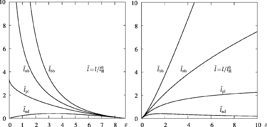
Figure 1: Distances as functions of $x$ (left) and $z$ (right).

In Figure 1 dependences of distances on the parameter $x$ (left) and redshift $z$ (right) are plotted.

Let us single out two moments related to distances. The first moment is when the distance according to the angular size takes the maximum value ($z=1.6302$), and the second moment is when the current metric distance turns out to be equal to the Hubble distance ($z=1.4233$). These data, and also for comparison, the moments corresponding to several characteristic values of the redshift, are given in Table 2 as a continuation of Table 1.

Table 2: Epochs associated with the characteristic values of redshift.

$x$	$z$	$\eta$	$t/t_{0}$	$t$ Gyrs	$t_{0}-t$
$0.0088000$	$1000$	$0.064629$	$2.9659\cdot 10^{-5}$	$4.0697\cdot 10^{-4}$	$13.721$
$0.017582$	$500$	$0.10796$	$9.4743\cdot 10^{-5}$	$1.3000\cdot 10^{-3}$	$13.720$
$0.087215$	$100$	$0.30606$	$1.2021\cdot 10^{-3}$	$0.016494$	$13.705$
$0.17272$	$50$	$0.45696$	$3.4279\cdot 10^{-3}$	$0.047036$	$13.675$
$0.80080$	$10$	$1.0642$	$0.034925$	$0.47924$	$13.242$
$0.97875$	$8$	$1.1841$	$0.047233$	$0.64811$	$13.074$
$3.3491$	$1.6302$	$2.2320$	$0.29360$	$4.0288$	$9.6930$
$3.6350$	$1.4233$	$2.3224$	$0.33008$	$4.5293$	$9.1925$
$2.2022$	$3$	$1.8084$	$0.15891$	$2.1806$	$0.11541$

Table 3 lists values of the distances to the points indicated in Tables 1 and 2.

Table 3: Distances to characteristic points of the Standard Model.

$z$	$\tilde{l}$	$\tilde{l}_{\rm ad}$	$\tilde{l}_{\rm nb}$	$\tilde{l}_{\rm bb}\phantom{\Bigl{|}}$
$\infty$	$3.322$	$0$	$\infty$	$\infty$
$5529$	$3.307$	$5.981\cdot 10^{-4}$	$245.9$	$18288$
$4057$	$3.302$	$8.138\cdot 10^{-4}$	$210.4$	$13401$
$2764$	$3.294$	$1.192\cdot 10^{-3}$	$173.2$	$9108$
$2339$	$3.290$	$1.406\cdot 10^{-3}$	$159.2$	$7700$
$2028$	$3.286$	$1.619\cdot 10^{-3}$	$148.0$	$6667$
$1169$	$3.265$	$2.790\cdot 10^{-3}$	$111.7$	$3821$
$1000$	$3.258$	$3.255\cdot 10^{-3}$	$103.1$	$3261$
$500$	$3.214$	$6.416\cdot 10^{-3}$	$71.95$	$1610$
$100$	$3.016$	$0.02987$	$30.31$	$304.7$
$50$	$2.865$	$0.05619$	$20.46$	$146.1$
$10$	$2.258$	$0.2053$	$7.490$	$24.83$
$8$	$2.138$	$0.2376$	$6.415$	$19.25$
$7.809$	$2.125$	$0.2412$	$6.306$	$18.72$
$3$	$1.514$	$0.3785$	$3.028$	$6.056$
$1.630$	$1.090$	$0.4146$	$1.768$	$2.868$
$1.423$	$1.000$	$0.4126$	$1.557$	$2.423$
$0.7264$	$0.6086$	$0.3525$	$0.7996$	$1.051$
$0.7255$	$0.6100$	$0.3524$	$0.7987$	$1.049$
$0.3702$	$0.3397$	$0.2479$	$0.3977$	$0.4655$
$0$	$0$	$0$	$0$	$0$

The velocity of change of the distance along the parallax coincides with $v/c$, since this distance itself coincides with the metric one. The rates of change of the remaining distances are determined from their definitions by differentiation with respect to time with a fixed spatial coordinate $\chi$. The expressions for these velocities are given in Table 4.

Table 4: Current velocities of change of distances.

Metric	ad	pl	nb	bb
$H_{0}l$	$H(\eta_{0}\!-\!\chi)l_{\rm ad}$	$H_{0}l_{\rm pl}$	$\displaystyle\frac{3H_{0}\!-\!H(\eta_{0}\!-\!\chi)}{\,\,\,\,\,\,\,\,2\phantom{bigl|}}l_{\rm nb}$	$[2H_{0}\!-\!H(\eta_{0}\!-\!\chi)]l_{\rm bb}$

The acceleration of cosmological expansion is found using the first equation in (11):

$$\dot{v}=\ddot{l}=\frac{{\rm d}^{2}}{{\rm d}t^{2}}l_{\rm H}^{0}a\chi=l_{\rm H}^{0}\ddot{a}\chi=\frac{\ddot{a}}{a}l=-\frac{4\pi G}{3}\rho_{\rm g}l=H_{\Lambda}^{2}\frac{x^{4}-\beta x/2-1}{x^{4}}l.$$ (46)

As already mentioned, in the gravitational density $\rho_{\rm g}=\rho_{\rm d}+2\rho_{\rm r}-2\rho_{\Lambda}$ densities $\rho_{\rm d}$ and $\rho_{\rm r}$ with the growth of the age of the universe decrease, but $\rho_{\Lambda}=\rho_{\Lambda}^{0}$. Therefore, in the numerator of the last fraction in (46), the role of the first term increases with time. At the present time ($x=x_{0}$) the gravitational density is negative: $\rho_{\rm g}^{0}=\rho_{\rm d}^{0}+2\rho_{\rm r}^{0}-2\rho_{\Lambda}^{0}=-1.0677\cdot 10^{-29}\,\,\hbox{{\rm g/cm}}^{3}$, so that the expansion occurs with an acceleration. But the acceleration at the current Hubble distance (speed equal to the speed of light) is only:

$$\dot{v}_{\rm H}^{0}=-\frac{4\pi G}{3}\rho_{\rm g}^{0}l_{\rm H}^{0}=\frac{H_{0}c}{2}(2\Omega_{\Lambda}^{0}-\Omega_{\rm d}^{0}-2\Omega_{{\rm r}\nu}^{0})=3.94\cdot 10^{-8}\,\,\hbox{{\rm cm/c}}^{2}\approx 4\,\,A\raise 11.0pt\hbox{\hskip-5.0pt\tiny$\circ$}\,/\hbox{{\rm c}}^{2}.$$ (47)

In the distant future at $t\to\infty$ ($z\to-1$, $\eta_{\infty}=4.4514$)

$$a\!=\!\frac{1}{1\!+\!z}\sim\left(\frac{\Omega_{\rm d}^{0}}{4\Omega_{\Lambda}^{0}}\right)^{1/3}e^{H_{\Lambda}t}\!=\!0.46000\,e^{H_{\Lambda}t},\,\,x\sim 4.0520\,e^{H_{\Lambda}t},\,\,\eta\sim\eta_{\infty}\!-\!2.5619e^{-H_{\Lambda}t}.$$ (48)

Thus, the scale of the universe will increase exponentially, that is a second inflation will take place, which we will discuss in more detail later. However, according to (48), really an exponential expansion will begin only for $t\sim t_{\Lambda}=1/H_{\Lambda}$. The time scale is $1/H_{0}=4.4081\cdot 10^{17}$s$=13.969$ Gyr, $t_{\Lambda}=1/H_{\Lambda}=5.1950\cdot 10^{17}$ s$=16.462$ Gyr. We also define the distance $l_{\Lambda}=c/H_{\Lambda}=l_{\rm H}^{0}/\sqrt{\Omega_{\Lambda}^{0}}=1.5574\cdot 10^{28}$ cm$=5.0473$ Gpc.

The speed of expansion of space at the Hubble distance is, by definition, equal to the speed of light. The velocity of change of the Hubble distance itself is found using equation (14):

$$\dot{l}_{\rm H}=\frac{{\rm d}}{{\rm d}t}\frac{c}{H}=-\frac{c}{H^{2}}\dot{H}=\frac{c}{H^{2}}\left(H^{2}+\frac{4\pi G}{3}\rho_{\rm g}\right)=c\left(1+\frac{1}{2}\frac{\rho_{\rm g}}{\rho_{c}}\right)=\frac{c}{2}\frac{4+3\beta x}{1+\beta x+x^{4}}.$$ (49)

According to this formula, at the beginning of the expansion the velocity is close to the two speeds of light, it is decreasing, and in the distant future it will approach zero. Acceleration at the Hubble distance increases with time, but remains finite:

$$\dot{v}_{\rm H}=-\frac{4\pi G}{3}\rho_{\rm g}l_{\rm H}=-\frac{4\pi G}{3}\rho_{\rm g}\frac{c}{H}=H_{\Lambda}c\frac{x^{4}-\beta x/2-1}{x^{2}\sqrt{1+\beta x+x^{4}}}\to H_{\Lambda}c=5.77A\raise 11.0pt\hbox{\hskip-5.0pt\tiny$\circ$}\,/\hbox{{\rm s}}^{2}.$$ (50)

Acceleration of the distance itself is negative:

$$\ddot{l}_{\rm H}=-\frac{c}{2}\frac{H_{\Lambda}}{x}\frac{\beta+16x^{3}+9\beta x^{4}}{(1+\beta x+x^{4})^{3/2}}\sim-cH_{\Lambda}\frac{9}{2}\frac{\beta}{x^{3}}.$$ (51)

From these formulas it is clear that, in order of magnitude, the accelerations are equal to the product of the speed of light by the modern Hubble constant or by the asymptotic value of the Hubble function: $cH_{0}=3\cdot 10^{10}\cdot 2.27\cdot 10^{-18}=6.81\cdot 10^{-8}$ cm/s², $cH_{\Lambda}=5.77\cdot 10^{-8}$ cm/s² (which coincides with the limit of (50)).

4 The second inflation and the second horizon

4.1 Visible and invisible parts of the universe

According to the theory of cosmological inflation, near the very beginning of the evolution of the universe, space exponentially expanded. The standard theory, as follows from (48), predicts that in the future, exponential expansion of space will continue, although at a much smaller rate. This expansion generates a new concept — a second horizon. The equation of motion of a photon traveling to the observer (that is, to us) is $\chi=\eta_{0}-\eta$; therefore, the place and time of its exit are related by the equality $\chi_{\hbox{\scriptsize e}}=\eta_{0}-\eta_{\hbox{\scriptsize e}}<\eta_{0}$. So the equation of motion can be rewritten as follows: $\chi=\chi_{\hbox{\scriptsize e}}+\eta_{\hbox{\scriptsize e}}-\eta$. Therefore, the distance from the observer to the photon traveling to him is:

$$l_{\rm rs}=l_{\rm H}^{0}a(\eta)(\chi_{\hbox{\scriptsize e}}+\eta_{\hbox{\scriptsize e}}-\eta).$$ (52)

The parameter $\eta$ is limited. For $t=\infty$, it is equal to $\eta_{\infty}=4.4514$. The equality of distance to zero $l_{\rm rs}=0$ is possible only if $\chi_{\hbox{\scriptsize e}}+\eta_{\hbox{\scriptsize e}}<\eta_{\infty}$; then there is another limitation on the ability to observe objects in the universe: along with the first horizon there is a second one.

The first horizon is called geometric (remember that the physical horizon is a sphere of the last scattering at $z\approx 1000$), while the second horizon can be called the kinematic or dynamic horizon. Other names are also used, borrowed from the terminology of the theory of black holes. The geometric horizon is called the horizon of particles, and the kinematic horizon is called the horizon of events.

At an arbitrary epoch, $\eta$, the first and second horizons are determined by the equations:

$$\chi_{\rm GHor}\!=\!\eta\!=\!H_{0}\!\int\limits_{0}^{a}\!\frac{{\rm d}a}{a^{2}H}\!=\!\eta_{*}I_{0}(x,\beta),\,\,\chi_{\rm KHor}\!=\!\eta_{\infty}\!-\!\eta\!=\!H_{0}\!\int\limits_{a}^{\infty}\!\frac{{\rm d}a}{a^{2}H}\!=\!\eta_{*}[I_{0}(\infty,\beta)\!-\!I_{0}(x,\beta)].$$ (53)

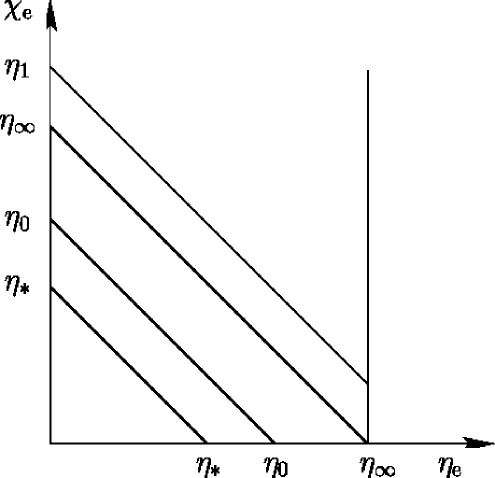
Figure 2: Visible and invisible parts of the universe.

In Figure 2 positions of the geometric horizon are indicated on the ordinate axis. The lines corresponding to this horizon are parallel to the abscissa. They rise with time, reflecting an expansion of the horizon. The second, kinematic, horizon is shown by a straight line connecting the abscissa and the ordinate, which are equal to $\eta_{\infty}$, while its specific position corresponds to the time on the abscissa axis. The paths of photons coming toward us, are represented by straight lines parallel to this straight line. Photons can start their journey from any point of the trajectory. Photons, for which $\eta_{\hbox{\scriptsize e}}+\chi_{\hbox{\scriptsize e}}<\eta_{\infty}$, that is, moving along straight lines lying below the straight line specified above, sooner or later will reach a place where the observer is located. For example, Figure 2 shows the paths of photons that have reached our place at time $\eta_{*}<\eta_{0}$ and at the current epoch $\eta_{0}$. If $\eta_{\hbox{\scriptsize e}}+\chi_{\hbox{\scriptsize e}}>\eta_{\infty}$, then photons with such coordinates do not ever reach our place. According to the equality $\eta_{\hbox{\scriptsize e}}+\chi_{\hbox{\scriptsize e}}=\eta_{\infty}$, it would seem that the photon still has to reach the observer, at least at an infinite time, but even such event is impossible.

From behind the first horizon, the radiation has not reached the observer yet. The second horizon separates the region of time and points from which radiation cannot reach the observer because the photons coming from there are moving away from the observer. This is true since space expands at speeds higher than the speed of light, and these speeds are increasing with time. Now we see the universe right up to the redshifts $z\approx 10$, but this is its past. The objects located now on the redshifts $z\geq 1.725$, we will never see.

Indeed, if a photon is now emitted toward us from a place with coordinate $\chi_{\rm o}$, then the distance to it at moment $\eta$ will be $l_{\rm ph}=l_{\rm H}^{0}a(\eta)(\chi_{\rm o}+\eta_{0}-\eta)$. This distance can become equal to zero at $\eta=\chi_{\rm o}+\eta_{0}$, and there must be $\chi_{\rm o}+\eta_{0}<\eta_{\infty}$. Thus, a boundary of the coordinate $\chi_{\rm o}$ for emitted now photons is $\chi_{\rm lim}^{0}=\eta_{\infty}-\eta_{0}=1.13$. The values of $x_{\rm lim}^{0}=3.23$, $z_{\rm lim}^{0}=1.725$, and $l_{\rm lim}^{0}=4.84$ Gpc$=l_{\rm KHor}^{0}$ correspond to this coordinate. The sphere of such a radius is the current second horizon. Thus, the radiation from the points now located at distances of $4.84$ Gpc from us will never reach us, even in the infinitely remote future.

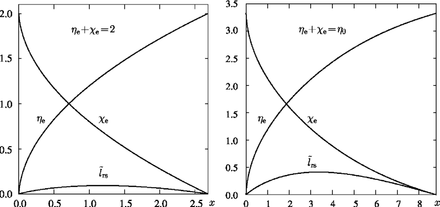
Figure 3: The paths of photons with arrival time at epochs: $\eta=2$ (left) and $\eta_{0}=3.3224$ (right).

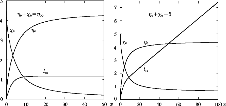
Figure 4: The paths of photons with “arrival” time at epochs: $\eta_{\infty}=4.4514$ (left) and $\eta=5$ (right).

Figure 3 shows distances $l_{\rm rs}$ to the photons arriving to the observer at the epoch when $\eta=2$ (Figure 3 left), and at the current epoch (Figure 3 right). In Figure 4 these distances are given for cases when the sum of the coordinates of time and location of the photon emission is equal to $\eta_{\infty}$ (Figure 4 left) and larger than that (Figure 4 right), both as a function of values of $x$. Figures also show curves reflecting the relationship between the time $\eta_{\hbox{\scriptsize e}}$ and the location $\chi_{\hbox{\scriptsize e}}$ of the photon emission.

Generally speaking, if a photon has emitted at a point where the expansion speed is greater than the speed of light, this does not necessarily mean that it will not reach us. As is known, cosmological expansion occurs in the same way with respect to all points of space, and it starts after a period of inflation with a very high speed (formally infinite, according to formula (34), which defines Big Bang), although in the beginning the expansion was slowing down. A photon emitted from far away, where the speed of expansion is large but closer than the horizon, still comes to us, because it gradually moves into layers of space expanding at a slower and slower rate. At some point its velocity toward us becomes zero, and then becomes negative, that is, it begins to approach us. However, it takes a long time for the photon to reach us. Consider, for example, the galaxy, observed by us now at redshift $z=3$, according to Table 2 moves away from us with a speed of $H_{0}l=c\tilde{l}=1.51c$, and earlier its speed was greater. At the same time, its radiation traveled to us for $11.5$ billion years, that is, we see this galaxy as it was in the distant past, when neither the Earth, nor even the Sun existed (but the galaxies and stars of the previous generations have already formed).

Figure 3 shows that for a photon emitted sufficiently early, its distance from us first increases, which means an expansion with speed larger than the speed of light, faster than the photon speed. From the point where the distance reaches a maximum, the photon begins to approach and finally comes to us. However, this is not possible, as shown in Figure 4, if $\eta_{\hbox{\scriptsize e}}+\chi_{\hbox{\scriptsize e}}\geq\eta_{\infty}$, even if the equality is true. Figure 4 left shows that a photon emitted at the second horizon, and then travels along it, would arrive at the observer after an infinite time; in fact, the photon only recedes along with the horizon. After an infinite time such a photon will be at a distance $l_{\Lambda}\approx 5.0$ Gpc, since the factor $\eta_{\infty}-\eta$ in the formula (52) at $\chi_{\hbox{\scriptsize e}}+\eta_{\hbox{\scriptsize e}}=\eta_{\infty}$ tends to zero if $t\to\infty$, while the factor $a(\eta)\to\infty$, but their product remains finite. A photon emitted at $\eta_{\hbox{\scriptsize e}}+\chi_{\hbox{\scriptsize e}}<\eta_{\infty}$ someday, maybe, after a very long time, will reach the current place of our civilization, but one emitted at $\eta_{\hbox{\scriptsize e}}+\chi_{\hbox{\scriptsize e}}>\eta_{\infty}$ will only recede from this place, and from some moment exponentially fast. The reason for this is the accelerated expansion of space. Thus, galaxies located on the second horizon and behind it will forever disappear from our field of view. These statements follow from the formulas given below.

4.2 Distances, velocities, and accelerations of horizons

Distances to horizons at an arbitrary epoch $\eta$ according to equations (53) are defined by the formulas:

$$\displaystyle l_{\rm GHor}=l_{\rm H}^{0}a(\eta)\eta=l_{\Lambda}xI_{0}(x,\beta),$$ (54)

$$\displaystyle l_{\rm KHor}=l_{\rm H}^{0}a(\eta)(\eta_{\infty}-\eta)=l_{\Lambda}x[I_{0}(\infty,\beta)-I_{0}(x,\beta)].$$ (55)

The sum of the horizon coordinates is constant at all times, and the sum of the distances to them is proportional to the scale factor. Both horizons expand. The speed of the geometric horizon exceeds by the speed of light the velocity of the place where the horizon is located at the moment $\dot{l}_{\rm GHor}=l_{\rm H}^{0}\dot{a}\eta+l_{\rm H}^{0}a\dot{\eta}=Hl_{\rm GHor}+c$. It expands with an acceleration. In contrast, the velocity of the kinematic horizon is less than the speed of its location by the speed of light: $\dot{l}_{\rm KHor}=l_{\rm H}^{0}\dot{a}(\eta_{\infty}-\eta)-l_{\rm H}^{0}a\dot{\eta}=Hl_{\rm KHor}-c$, and its expansion slows down.

Asymptotes of distances to horizons and their velocities at $t\to\infty$, $a\to\infty$, $z\to-1$ are determined taking into consideration that $I_{0}(\infty,\beta)=0.42880$ and $\displaystyle I_{0}(\infty,\beta)-I_{0}(x,\beta)\sim\frac{1}{x}\left(1-\frac{1}{8}\frac{\beta}{x^{3}}\right)$:

$$\displaystyle l_{\rm GHor}\sim l_{\rm H}^{0}\eta_{*}\,I_{0}(\infty,\beta)a=5.9\cdot 10^{28}a\,\,\hbox{{\rm cm}}\sim 2.7\cdot 10^{28}e^{H_{\Lambda}t}\,\,\hbox{{\rm cm}}\to\infty,$$ (56)

$$\displaystyle l_{\rm KHor}\to l_{\Lambda}=\frac{c}{H_{\Lambda}}=1.56\cdot 10^{28}\,\,\hbox{{\rm cm}}=5.05\,\,\hbox{{\rm Gpc}}.$$ (57)

The current distance to the geometric horizon is $\displaystyle l_{\rm GHor}^{0}\!=\!l_{\rm H}^{0}\eta_{0}\!=\!3.32\,l_{\rm H}^{0}\!=\!4.39\cdot 10^{28}$ cm$\!=\!14.2$ Gpc. The velocity near the horizon is $v_{\rm GHor}^{0}=c\eta_{0}=3.32c$, and the velocity of the expansion of the horizon is $\dot{l}_{\rm GHor}^{0}=4.32c$. The horizon will pass $4.32$ light years in one year, which is equal to $1.33$ pc, so that $1$ Gpc will be added to the current $14.2$ Gpc in $0.755\cdot 10^{9}$ years, if the speed of the horizon is equal to its current velocity, and in $0.741\cdot 10^{9}$ years, if the increase of the velocity is taken into account.

The current distance to the second horizon is $l_{\rm KHor}^{0}\!=\!l_{\rm H}^{0}(\eta_{\infty}\!-\!\eta_{0})\!=1.49\cdot 10^{28}$ cm$=\!4.84$ Gpc, the limit to this distance coincides with the Hubble limit: $\displaystyle l_{\rm KHor}\to\frac{l_{\rm H}^{0}}{\sqrt{\Omega_{\Lambda}^{0}}}=\frac{c}{H_{\Lambda}}=5.05$ Gpc. The current speed of expansion of the location of this horizon is $c(\eta_{\infty}-\eta_{0})=1.13c$, and the speed of recession of the kinematic horizon from us now is $0.13c$.

The velocities of the horizons at an arbitrary moment and their asymptotics for $t\to\infty$ and $x\sim 5.0\cdot e^{H_{\Lambda}t}\to\infty$:

$$\displaystyle\dot{l}_{\rm GHor}\!=\!l_{\rm H}^{0}(\dot{a}\eta\!+\!a\dot{\eta})\!=\!Hl_{\rm GHor}\!+\!c\!=\!c\left[\frac{\sqrt{1\!+\!\beta x\!+\!x^{4}}}{x}I_{0}(x,\beta)\!+\!1\right]\sim cxI_{0}(\infty,\beta),$$ (58)

$$\displaystyle\dot{l}_{\rm KHor}=c\left[\frac{\sqrt{1+\beta x+x^{4}}}{x}[I_{0}(\infty,\beta)-I_{0}(x,\beta)]-1\right]\sim\frac{3}{8}\frac{\beta}{x^{3}}c.$$ (59)

It is interesting to note that all points with fixed coordinate $\chi$ begin (at the initial instant of the expansion) to move away from each other at an infinite speed (according to (34), $\displaystyle\dot{a}=\dot{x}/x_{0}=(H_{\Lambda}/x_{0})\sqrt{1+\beta x+x^{4}}/x$). The geometric horizon begins to expand with velocity $2c$, as does the Hubble distance, but the evolution of their velocities is opposite (see formulas (49) and (56)). For small $x$, the velocity $\dot{l}_{\rm GHor}$ grows very fast, while the velocity $\dot{l}_{\rm H}$ rapidly decreases, so that at $x=0.03$ they become equal to $2.50c$ and $1.56c$, respectively. The second horizon begins the expansion, like all ordinary points of space, with an infinite value of speed, which then decreases very fast.

Accelerations have evolution similar to speeds:

$$\displaystyle\ddot{l}_{\rm GHor}\!=\!l_{\rm H}^{0}\left(\ddot{a}\eta\!+\!2\dot{a}\dot{\eta}\!+\!a\ddot{\eta}\right)\!=\!\frac{\ddot{a}}{a}l_{\rm GHor}\!+\!l_{\rm H}^{0}\left(2\dot{a}\frac{H_{0}}{a}\!-\!a\frac{H_{0}}{a^{2}}\dot{a}\right)\!=\!-\frac{4\pi G}{3}\rho_{\rm g}l_{\rm GHor}\!+\!cH$$

$$\displaystyle=cH_{\Lambda}\left[\frac{\sqrt{1+\beta x+x^{4}}}{x^{2}}+\frac{x^{4}-\beta x/2-1}{x^{3}}I_{0}(x,\beta)\right]\sim cH_{\Lambda}I_{0}(\infty,\beta)x,$$ (60)

$$\displaystyle\ddot{l}_{\rm KHor}=l_{\rm H}^{0}\left[\ddot{a}(\eta_{\infty}-\eta)-2\dot{a}\dot{\eta}-a\ddot{\eta}\right]=\frac{\ddot{a}}{a}l_{\rm KHor}-l_{\rm H}^{0}\left(2\dot{a}\frac{H_{0}}{a}-a\frac{H_{0}}{a^{2}}\dot{a}\right)$$

$$\displaystyle=-\frac{4\pi G}{3}\rho_{\rm g}l_{\rm H}^{0}\frac{x}{x_{0}}\frac{I_{0}(\infty,\beta)-I_{0}(x,\beta)}{(\Omega_{\rm r}^{0}\Omega_{\Lambda}^{0})^{1/4}}-cH$$

$$\displaystyle=cH_{\Lambda}\left[\frac{x^{4}-\beta x/2-1}{x^{3}}[I_{0}(\infty,\beta)\!-\!I_{0}(x,\beta)]\!-\!\frac{\sqrt{1+\beta x+x^{4}}}{x^{2}}\right]\sim-\frac{9}{8}\frac{\beta}{x^{3}}cH_{\Lambda}.$$ (61)

At $x=x_{0}$, we obtain the current values of the velocities (see above) and accelerations: $\ddot{l}_{\rm GHor}^{0}=3.45H_{\Lambda}c=19.9\cdot 10^{-8}$  cm/c², $\ddot{l}_{\rm KHor}^{0}=-1.95\,H_{\Lambda}c=-11.3\cdot 10^{-8}$  cm/c².

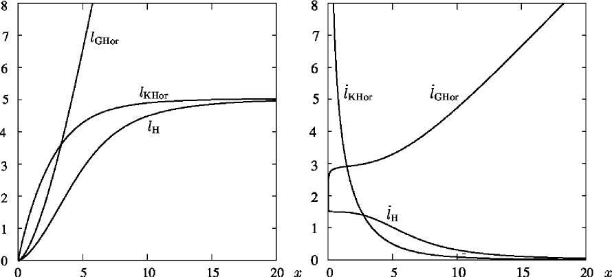
Figure 5: Left: Hubble distance and distances to the horizons in Gpc. Right: Speeds of change of distances in units of the speed of light. (right).

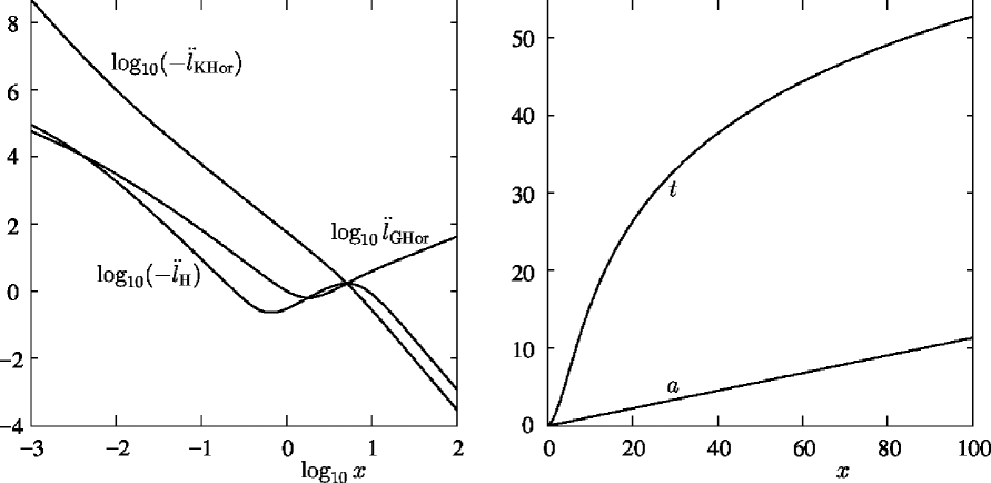
Figure 6: Left: Accelerations of the horizons and the Hubble distance. Right: Values of $a$ and $t$ as functions of $x$.

The speed of the first horizon increases, while that of the second horizon decreases. During the entire period of action of the cosmological acceleration ($6.5\cdot 10^{9}$ years), the velocity of the first horizon increased from $3.31\,c$ (by the value of $\eta$ for $\rho_{\rm g}=0$ in Table 1) to the current velocity of $4.32\,c$, and the speed of the second horizon decreased from $0.479\,c$ to $0.129\,c$.

Figure 5, left represents the distances to the horizons, and Figure 5, right shows their velocities as a function of the parameter $x$. The figures give the same values for the Hubble distance. All distances are given in Gpc, and velocities are indicated in units of the speed of light. At first, until $\eta_{\infty}-\eta>\eta$, the distance to the second horizon is greater than that to the first horizon. The horizons intersected when $\eta_{\rm crs}=\eta_{\infty}/2=2.23$, $x_{\rm crs}=4.08$, $z_{\rm crs}=1.677$ at the epoch $t_{\rm crs}=3.93$ billion years from the beginning, that is $t_{0}-t_{\rm crs}=9.80$ billion years ago (earlier than the acceleration began), when the distance to the horizons was $3.58$ Gpc. Prior to this, the first horizon determined the initial possibility to do observations (if there were observers at that time). Since then, the second horizon has become closer to us and it is the second horizon that limits the area of the visible universe.

Figure 6, left plots the accelerations of the horizons and Hubble distance, measured in units of $cH_{\Lambda}$, on a logarithmic scale. Only the acceleration of the second horizon is a monotonic function; $\ddot{l}_{\rm GHor}$ has a minimum, while $\ddot{l}_{\rm H}$ has both a minimum and a maximum. The figures show a linear increase of the acceleration $\ddot{l}_{\rm GHor}$ with $x>1$, and the equality of the rates of decrease of the accelerations $\ddot{l}_{\rm H}$ and $\ddot{l}$ according to the asymptotes (51) and (4.2). Figure 6, right shows the relationship of the scale factor $a$ and cosmological time $t$ with the parameter $x$.

4.3 Connection with extraterrestrial civilizations

Suppose that at our epoch ($t=t_{0},\,\,\eta=\eta_{0}$) a radio signal is emitted in some direction. The distance to it increases and for a value of the time coordinate $\eta$ the distance will be equal to $l_{\rm ph}=l_{\rm H}^{0}a(\eta)(\eta-\eta_{0}),\,\,\eta\geq\eta_{0}$. Its speed includes both the speed of expansion and the speed of light:

$$\dot{l}_{\rm ph}=l_{\rm H}^{0}\dot{a}(\eta-\eta_{0})+l_{\rm H}^{0}a\dot{\eta}=Hl_{\rm ph}+c.$$ (62)

For brevity, we omit the factor $l_{\rm H}^{0}$, which means that we use distances measured in units of the Hubble distance. On the way, the signal meets objects with a fixed spatial coordinate $\chi_{\rm O}=\eta_{0}-\eta_{\rm O}$. Distances to them grow only due to the cosmological expansion, that is, increasing scale factor: $\tilde{l}_{\rm O}=a(\eta)(\eta_{0}-\eta_{\rm O})$. The signal catches up with the object when their distances from us becomes equal, which occurs at the moment $\eta_{\rm mt}$, when $\eta_{\rm mt}-\eta_{0}=\eta_{0}-\eta_{\rm O}$, $\eta_{\rm mt}=2\eta_{0}-\eta_{\rm O}$, therefore $\tilde{l}_{\rm ph}=\tilde{l}_{\rm O}=a(2\eta_{0}-\eta_{\rm O})(\eta_{0}-\eta_{\rm O})$. Since $\eta_{\rm mt}$ can not exceed $\eta_{\infty}$, the signal can meet for a finite (although, perhaps, very large) time only those objects which have the coordinate equal to $\chi_{\rm O}<\eta_{\infty}-\eta_{0}=1.13$. This implies that the coordinate has the same boundary as a photon traveling toward us. This boundary is the second horizon (see above), and $\eta_{\rm O}>\eta_{\rm lim}=2\eta_{0}-\eta_{\infty}=2.19$.

Table 5: Objects along the signal path.

$\eta_{\rm O}$	$x_{\rm O}$	$a_{\rm O}$	$z_{\rm O}$	$l_{\rm O}^{0}$ Гпк	$t_{\rm O}$
$1.99$	$2.67$	$0.303$	$2.30$	$5.69$	$2.89$
$2.19$	$3.23$	$0.367$	$1.73$	$4.84$	$3.83$
$2.39$	$3.87$	$0.440$	$1.28$	$3.98$	$4.95$
$2.59$	$4.60$	$0.523$	$0.913$	$3.12$	$6.29$
$2.79$	$5.46$	$0.620$	$0.613$	$2.27$	$7.88$
$2.99$	$6.49$	$0.737$	$0.357$	$1.41$	$9.77$

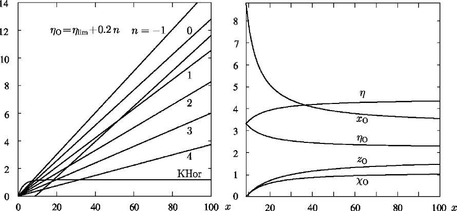
Figure 7: Left: Path of the signal to objects.   Right: Objects reachable by the signal.

Figure 7, left contains lines that plot the dependence of the distance $l_{\rm O}$ on the coordinate $x$ for six objects. Positions of the signal path and the kinematic horizon are indicated as well. The objects are characterized by values of $\eta_{\rm O}=\eta_{\rm lim}+0.2n$, $n=-1(1)4$. The corresponding values of $x_{\rm O}$, the scale factor $a_{\rm O}=a(\eta_{\rm O})$, and the redshift $z_{\rm O}$, as well as the current distances to these objects $l_{\rm O}^{0}$, are given in Table 5. It can be seen from the figure that the emitted signal reaches the objects only when $n=1,2,3,4$. The signal comes earlier to objects with larger values of $\eta_{\rm O}$, and hence smaller values of $z_{\rm O}$ and $l_{\rm O}$. These objects are located closer to the place and moment of the signal output at the moment of its emission. The signal only catches up to objects with $n=3$ and $4$, for which the values of $\eta_{\rm O}$ are equal to $2.79$ and $2.99$, respectively, before they cross the second horizon. The condition of this is $\eta_{0}-\eta_{\rm O}<\eta_{\infty}-2\eta_{\rm O}+\eta_{\rm O}$, that is, $\displaystyle\eta_{\rm O}>\eta_{\rm h}=\frac{3\eta_{0}-\eta_{\infty}}{2}=2.758$. The distance between the object, which is now almost on the second horizon (the current distance to it is $4.84$ Gpc and its redshift is $1.72$), and the signal for $\tilde{l}_{\rm O}^{0}=\eta_{\infty}-\eta_{0}-\varepsilon$, $\eta_{\rm O}=\eta_{\rm lim}+\varepsilon$ is:

$$l_{\rm O}\!-\!l_{\rm ph}\!=\!l_{\rm H}^{0}a(\eta)(\eta_{0}\!-\!\eta_{\rm lim}\!-\!\varepsilon)\!-\!l_{\rm H}^{0}a(\eta)(\eta\!-\!\eta_{0})\!=\!l_{\rm H}^{0}a(\eta)(\eta_{\infty}\!-\!\varepsilon\!-\!\eta)\!\sim\!\frac{c}{H_{\Lambda}}\frac{\eta_{\infty}\!-\!\varepsilon\!-\!\eta}{\eta_{\infty}-\eta},$$ (63)

because, according to eqs. (35) and (38), $\eta\!\sim\!\eta_{\infty}\!-\!\eta_{*}/x$, $a(\eta)\!=\!x/x_{0}\!\sim\!1/\left[\sqrt{\Omega_{\Lambda}^{0}}(\eta_{\infty}\!-\!\eta)\right]$ for $x\to\infty$, $\eta_{\infty}-\eta\ll 1$. The difference (63) tends to zero for $\eta\to\eta_{\infty}-\varepsilon$, if $\varepsilon>0$. Thus, in agreement with Figure 7, left, the signal will still reach any object if this object is located at least slightly closer than the second horizon. The time that the signal needs to meet the object is $t\sim\ln(1/\varepsilon)$. If the object is located on the horizon ($\varepsilon=0$) there remains an insurmountable distance $c/H_{\Lambda}=5.05$ Gpc. The distance will only increase with time between the signal emitted now and objects located currently behind the second horizon. In addition, it will increase asymptotically as an exponential function. These objects are carried away precisely by the exponential expansion, that is, by the repulsion of the dark energy. In models without repulsion the second horizon does not appear.

Figure 7, right shows the dependences of the coordinates $x_{\rm O}$, $\eta_{\rm O}$ и $\chi_{\rm O}=\eta_{0}-\eta_{\rm O}$, as well as redshifts $z_{\rm O}$ of objects, which the signal will reach at the moment corresponding to its coordinate $x$. The figure plots also the dependence of the time coordinate $\eta$ on $x$. The signal emitted now will reach the second horizon when

$$l_{\rm ph}=l_{\rm H}^{0}a(\eta_{\rm h})(\eta_{\rm h}-\eta_{0})=l_{\rm KHor}=l_{\rm H}^{0}a(\eta_{\rm h})(\eta_{\infty}-\eta_{\rm h}),\quad\eta_{\rm h}=\frac{\eta_{0}+\eta_{\infty}}{2}=3.89.$$ (64)

The corresponding values are $x_{\rm h}=18.3$, $l_{\rm ph}=l_{\rm KHor}=5.02$ Gpc, and $t_{\rm h}=24.9$ Gyr. At this time an object with initial coordinate $x_{\rm O}=5.30$ will approach the horizon. This coordinate corresponds to $a_{\rm O}=0.601$, $z_{\rm O}=0.663$, and an initial distance to us of $l_{\rm O}^{0}=l_{\rm H}^{0}(\eta_{0}-\eta_{\rm O})=1.45$ Gpc, because if $l_{\rm O}=l_{\rm ph}=l_{\rm KHor}$ then $\eta_{0}-\eta_{\rm O}=\eta_{\rm h}-\eta_{0}=\eta_{\infty}-\eta_{\rm h}$ and $\eta_{\rm O}=(3\eta_{0}-\eta_{\infty})/2=2.76$.

The signal sent by us can reach distances only up to $\approx$5 Gpc with a hope to get an answer. Exponential expansion of space entrains radiation, both coming from us and directed toward us. Nevertheless, $5$ Gpc is a very large distance, inside the sphere of such a radius there are many galaxies. If the signal hits a planet populated by intelligent creatures who have reached an advanced stage of civilization, they will receive it, understand, determine the direction from what it came, and answer. Then their signal will approach that place where we (people) were when we sent the first signal. The distance of their signal to us will change according to the formula: $\tilde{l}_{\rm ret}=a(\eta)(\eta_{\rm mt}-\eta_{0}-(\eta-\eta_{\rm mt})=a(\eta)(3\eta_{0}-2\eta_{\rm O}-\eta)$. An answer will come to us at the moment $\eta_{\rm ret}=3\eta_{0}-2\eta_{\rm O}$. If we want that an answer would come at a moment $\eta_{\rm ret}^{0}$, $\eta_{0}<\eta_{\rm ret}^{0}<\eta_{\infty}$, then such a civilization should have $\eta_{\rm O}>(3\eta_{0}-\eta_{\rm ret}^{0})/2$ and $\chi_{\rm O}<(\eta_{\rm ret}^{0}-\eta_{0})/2$. In an extreme case, if we assume that $\eta_{\rm ret}^{0}=\eta_{\infty}$ then the condition imposes a restriction on the coordinate $\eta_{\rm O}$: $\displaystyle\eta_{\rm O}>(3\eta_{0}-\eta_{\infty})/2$. This restriction coincides with the condition that the signal reaches the object (civilization) before the latter reaches the second horizon. The restriction on the spatial coordinate is as it was previously: $\chi_{\rm O}=\eta_{0}-\eta_{\rm O}<(\eta_{\infty}-\eta_{0})/2$.

These arguments are purely theoretical, since sending a signal makes sense only to objects located not farther than several dozen light years, otherwise waiting for a possible answer will take too long a time. In addition, signals either need to be sent in a very narrow solid angles, or they should possess very high energy to penetrate to a sufficiently large distance. Although the above arguments have a purely theoretical or even academic character, they establish fundamental, limiting restrictions imposed by the model. They can be related either to epochs when our civilization on the Earth has not existed yet, or has not been able to realize connections with other civilizations, or to the epochs when the Sun and Earth will not exist in their current form anymore. However, these same arguments apply to any arbitrary point of the universe and to civilizations that may arise and prosper at any time.

5 Conclusion

Therefore, our paper gives a quantitative description of geometric and kinematic properties of the model, which is now considered as the most adequate model of the existing universe. Acknowledgements

SJ acknowledges a support from St. Petersburg University research grant 6.38.335.2015.

References

• [1] Zeldovich Ya.B., Novikov I.D. 1975. The Structure and Evolution of the Universe. University of Chicago Press, Chicago, 1983.
• [2] Narlikar J. V. Introduction to Cosmology. Cambridge, Cambridge University Press, 1993.
• [3] Misner T.w., Thorn K.S., Wheeler J.A. Gravitation. San Francisco, Freeman, 11972.
• [4] Weinberg S. Gravitation and Cosmology: Principles and Applications of the General Theory of Relativity. New York, John Wiley and Sons, Inc., 1972.
• [5] Gorbunov D.C., Rubakov V.A. Introduction to the Theory of the Early Universe. The Theory of Hot Big Bang. М., URSS, 2008.
• [6] R.Alpher, R.Herman. Ann. Rev. Nucl. Sci. 2, 1, 1953.
• [7] Hinshaw G., Larson D., Komatsu E., et al. Nine-year Wilkinson Microwave Anisotropy Probe (WMAP) observations: cosmological parameters results. Astrophysical Journal Supplemet Series, 208, 19 (25 pp.) 2013.