Spectral Simplicity of Apparent Complexity, Part II:
Exact Complexities and Complexity Spectra

Abstract

The meromorphic functional calculus developed in Part I overcomes the nondiagonalizability of linear operators that arises often in the temporal evolution of complex systems and is generic to the metadynamics of predicting their behavior. Using the resulting spectral decomposition, we derive closed-form expressions for correlation functions, finite-length Shannon entropy-rate approximates, asymptotic entropy rate, excess entropy, transient information, transient and asymptotic state uncertainty, and synchronization information of stochastic processes generated by finite-state hidden Markov models. This introduces analytical tractability to investigating information processing in discrete-event stochastic processes, symbolic dynamics, and chaotic dynamical systems. Comparisons reveal mathematical similarities between complexity measures originally thought to capture distinct informational and computational properties. We also introduce a new kind of spectral analysis via coronal spectrograms and the frequency-dependent spectra of past-future mutual information. We analyze a number of examples to illustrate the methods, emphasizing processes with multivariate dependencies beyond pairwise correlation. An appendix presents spectral decomposition calculations for one example in full detail.

The prequel laid out a new toolset that allows one to analyze in detail how complex systems store and process information. Here, we use the tools to calculate in closed form almost all complexity measures for processes generated by finite-state hidden Markov models. Helpfully, the tools also give a detailed view of how subprocess components contribute to a process’ informational architecture. As an application, we show that the widely-used methods based on Fourier analysis and power spectra fail to capture the structure of even very simple structured processes. We introduce the spectrum of past-future mutual information and show that it allows one to detect such structure.

I Introduction

Tracking the evolution of a complex system, a time series of observations often appears quite complicated in the sense of temporal patterns, stochasticity, and behavior that require significant resources to predict. Such complexity arises from many sources. Apparent complexity, even in simple systems, can be induced by practical measurement and analysis issues, such as small sample size, inadequate collection of probes, noisy or systematically distorted measurements, coarse-graining, out-of-class modeling, nonconvergent inference algorithms, and so on. The effects can either increase or decrease apparent complexity, as they add or discard information, hiding the system of interest from an observer to one degree or another. Assuming perfect observation, complexity can also be inherent in nonlinear stochastic dynamical processes—deterministic chaos, superexponential transients, high state-space dimension, nonergodicity, nonstationarity, and the like. Even in ideal settings, the smallest sufficient set of a system’s maximally predictive features is generically uncountable, making approximations unavoidable, in principle [1]. With nothing else said, these facts obviate physical science’s most basic goal—prediction—and, without that, they preclude understanding how nature works. How can we make progress?

The prequel, Part I, argued that this is too pessimistic a view. It introduced constructive results that address hidden structure and the challenges associated with predicting complex systems. Part I showed that questions regarding correlation, predictability, and prediction each require their own analytical structures, as long as one can identify a system’s hidden linear dynamic. It distinguished two genres of quantitative question: (i) cascading, in which the influence of an initial preparation cascades through state-space as time evolves, affecting the final measurement, and (ii) accumulating, in which statistics are gathered during such cascades. Part I identified the linear algebraic structure underlying each kind.

Part I explained that the hidden linear dynamic in systems induces a nondiagonalizable metadynamics, even if the dynamics are diagonalizable in their underlying state-space. Assuming normal and diagonalizable dynamics, so familiar in mathematical physics, simply fails in this setting. Thus, nondiagonalizable dynamics present an analytical roadblock. Part I reviewed a calculus for functions of nondiagonalizable operators—the recently developed meromorphic functional calculus of Ref. [2]—that directly addresses nondiagonalizability, giving constructive calculational methods and algorithms.

Along the way, Part I reviewed relevant background in stochastic processes and their complexities and the hidden Markov models (HMMs) that generate them. It delineated several classes of HMMs—Markov chains, unifilar HMMs, and nonunifilar HMMs. It also reviewed their mixed-state presentations (MSPs)—HMM generators of a process that track distributions induced by observation. Related constructions included the HMM and $\epsilon$-machine synchronizing MSPs, generator mixed-functional presentations, and cryptic-operator presentations. MSPs are key to calculating complexity measures within an information-theoretic framing. Part I then showed how each complexity measure reduces to a linear algebra of an appropriate HMM adapted to the cascading- or accumulating-question genre. It summarized the meromorphic functional calculus and several of its mathematical implications in relation to projection operators. Part I also highlighted a spectral weighted directed-graph theory that can give useful shortcuts for determining a process’ spectral decomposition. Part II here uses Part I’s notation and assumes familiarity with its results.

With Part I’s toolset laid out, Part II now derives the promised closed-form complexities of a process. Section §II investigates the range of possible behaviors for correlation and myopic uncertainty via convergence to asymptotic correlation and asymptotic entropy rates. Section §III then considers measures related to accumulating quantities during the transient relaxation to synchronization. Section §IV introduces closed-form expressions for a wide range of complexity measures in terms of the spectral decomposition of a process’ dynamic. It also introduces complexity spectra and highlights common simplifications for special cases, such as almost diagonalizable dynamics. Section §V gives a new kind of signal analysis in terms of coronal spectrograms. A suite of examples in §VI and §VII ground the theoretical developments and are complemented with an in-depth pedagogical example worked out in App. §A. Finally, we conclude with a brief retrospective of Parts I and II and give an eye towards future applications.

II Correlation and Myopic Uncertainty

Using Part I’s methods, our first step is to solve for the correlation function:

$$\gamma(L) =\left\langle\overline{{X}}_{t}{X}_{t+L}\right\rangle_{t}$$ (1)

and the myopic uncertainty or finite-history Shannon entropy rate:

$$h_{\mu}(L) =\operatorname{H}\left[X_{L}\middle|X_{1:L}\right]~{}.$$ (2)

A comparison is informative. We then determine the asymptotic correlation and myopic uncertainty from the resulting finite-$L$ expressions.

II.1 Nonasymptotics

A central result in Part I was the spectral decomposition of powers of a linear operator $A$, even if that operator is nondiagonalizable. Recall that for any $L\in\mathbb{C}$:

$$A^{L} =\Biggl{[}\sum_{\lambda\in\Lambda_{A}\atop\lambda\neq 0}\sum_{m=0}^{\nu_{\lambda}-1}\binom{L}{m}\lambda^{L-m}A_{\lambda,m}\Biggr{]}$$

$$\qquad+\left[0\in\Lambda_{A}\right]\sum_{m=0}^{\nu_{0}-1}\delta_{L,m}A_{0}A^{m}~{},$$ (3)

where $\binom{L}{m}$ is the generalized binomial coefficient:

$$\binom{L}{m} =\frac{1}{m!}\prod_{n=1}^{m}(L-n+1)~{},$$ (4)

$\binom{L}{0}=1$, and $[0\in\Lambda_{A}]$ is the Iverson bracket. The latter takes on value $1$ if zero is an eigenvalue of $A$ and $0$ if not.

In light of this, the autocorrelation function $\gamma(L)$ is simply a superposition of weighted eigen-contributions. Part I showed that Eq. (1) has the operator expression:

$$\gamma(L)=\bra{\pi\overline{\mathcal{A}}}T^{|L|-1}\ket{\mathcal{A}\mathbf{1}}~{},$$

where $T$ is the transition dynamic, $\mathcal{A}$ is the output symbol alphabet, and we defined the row vector:

$$\bra{\pi\overline{\mathcal{A}}} =\bra{\pi}\Big{(}\sum_{{x}\in\mathcal{A}}\overline{{x}}T^{({x})}\Big{)}$$

and the column vector:

$$\ket{\mathcal{A}\mathbf{1}} =\Big{(}\sum_{{x}\in\mathcal{A}}{x}T^{({x})}\Big{)}\ket{\mathbf{1}}~{}.$$

Substituting Part I’s spectral decomposition of matrix powers, Eq. (3) above, directly leads to the spectral decomposition of $\gamma(L)$ for nonzero integer $L$:

$$\gamma(L) =\sum_{\lambda\in\Lambda_{T}\atop\lambda\neq 0}\sum_{m=0}^{\nu_{\lambda}-1}\bra{\pi\overline{\mathcal{A}}}T_{\lambda,m}\ket{\mathcal{A}\mathbf{1}}\binom{|L|-1}{m}\lambda^{|L|-1-m}$$

$$\qquad+[0\in\Lambda_{T}]\sum_{m=0}^{\nu_{0}-1}\bra{\pi\overline{\mathcal{A}}}T_{0}T^{m}\ket{\mathcal{A}\mathbf{1}}\delta_{|L|-1,m}$$ (5)

$$=\gamma_{\rightsquigarrow}(L)+\gamma_{\multimap}(L)~{}.$$ (6)

We denote the persistent first term of Eq. (5) as $\gamma_{\rightsquigarrow}$, and note that it can be expressed:

$$\gamma_{\rightsquigarrow}(L) =\bra{\pi\overline{\mathcal{A}}}T^{\mathcal{D}}TT^{|L|-1}\ket{\mathcal{A}\mathbf{1}}$$

$$=\bra{\pi\overline{\mathcal{A}}}T^{\mathcal{D}}T^{|L|}\ket{\mathcal{A}\mathbf{1}}~{},$$

where $T^{\mathcal{D}}$ is $T$’s Drazin inverse. We denote the ephemeral second term as $\gamma_{\multimap}$, which can be written as:

$$\gamma_{\multimap}(L)=\bra{\pi\overline{\mathcal{A}}}T_{0}T^{|L|-1}\ket{\mathcal{A}\mathbf{1}}~{},$$

where $T_{0}$ is the eigenprojector associated with the eigenvalue of zero; $T_{0}=\bm{0}$ if $0\notin\Lambda_{T}$.

From Eq. (5), it is now apparent that the index of $T$’s zero eigenvalue gives a finite-horizon contribution ($\gamma_{\multimap}$) to the autocorrelation function. Beyond index $\nu_{0}$ of $T$, the only $L$-dependence comes via a weighted sum of terms of the form $\binom{|L|-1}{m}\lambda^{|L|-1-m}$—polynomials in $L$ times decaying exponentials. The set $\bigl{\{}\bra{\pi\overline{\mathcal{A}}}T_{\lambda,m}\ket{\mathcal{A}\mathbf{1}}\bigr{\}}$ simply weights the amplitudes of these contributions. In the familiar diagonalizable case, the behavior of autocorrelation is simply a sum of decaying exponentials $\lambda^{|L|}$.

Similarly, in light of Part I’s expression for the myopic entropy rate in terms of the MSP—starting in the initial unsynchronized mixed-state $\pi$ and evolving the state of uncertainty via the observation-induced MSP transition dynamic $W$:

$$h_{\mu}(L) =\bra{\delta_{\pi}}W^{L-1}\ket{\operatorname{H}(W^{\mathcal{A}})}$$ (7)

—and its spectral decomposition of $A^{L}$, we find the most general spectral decomposition of the myopic entropy rates $h_{\mu}(L)$ to be:

$$h_{\mu}(L) =\sum_{\lambda\in\Lambda_{W}\atop\lambda\neq 0}\sum_{m=0}^{\nu_{\lambda}-1}\bra{\delta_{\pi}}W_{\lambda,m}\ket{\operatorname{H}(W^{\mathcal{A}})}\binom{L-1}{m}\lambda^{L-1-m}$$

$$+\left[0\in\Lambda_{W}\right]\sum_{m=0}^{\nu_{0}-1}\delta_{L-1,m}\bra{\delta_{\pi}}W_{0}W^{m}\ket{\operatorname{H}(W^{\mathcal{A}})}$$ (8)

$$=h_{\rightsquigarrow}(L)+h_{\multimap}(L)~{}.$$ (9)

We denote the persistent first term of Eq. (8) as $h_{\rightsquigarrow}$, and note that it can be expressed directly as:

$$h_{\rightsquigarrow}(L) =\bra{\delta_{\pi}}W^{\mathcal{D}}WW^{L-1}\ket{\operatorname{H}(W^{\mathcal{A}})}$$

$$=\bra{\delta_{\pi}}W^{\mathcal{D}}W^{L}\ket{\operatorname{H}(W^{\mathcal{A}})}~{},$$

where $W^{\mathcal{D}}$ is the Drazin inverse of the mixed-state-to-state net transition dynamic $W$. We denote the ephemeral second term as $h_{\multimap}$, which can be written as:

$$h_{\multimap}(L)=\bra{\delta_{\pi}}W_{0}W^{L-1}\ket{\operatorname{H}(W^{\mathcal{A}})}~{}.$$

From Eq. (8), we see that the index of $W$’s zero eigenvalue gives a finite horizon contribution ($h_{\multimap}$) to the myopic entropy rate. Beyond index $\nu_{0}$ of $W$, the only $L$-dependence comes via a weighted sum of terms of the form $\binom{L-1}{m}\lambda^{L-1-m}$—polynomials in $L$ times decaying exponentials. The set $\bigl{\{}\bra{\delta_{\pi}}W_{\lambda,m}\ket{\operatorname{H}(W^{\mathcal{A}})}\bigr{\}}$ weights the amplitudes of these contributions.

For stationary processes we anticipate that, for all $\zeta\in\{\lambda\in\Lambda_{W}:|\lambda|=1,\lambda\neq 1\}$, $\bra{\delta_{\pi}}W_{\zeta}=\mathbf{0}$ and thus $\bra{\delta_{\pi}}W_{\zeta}\ket{\operatorname{H}(W^{\mathcal{A}})}=0$. Hence, we can save ourselves from superfluous calculation by excluding the nonunity eigenvalues on the unit circle, when calculating the myopic entropy rate for stationary processes. In the diagonalizable case, again, its behavior is simply a sum of decaying exponentials $\lambda^{L}$.

In practice, $\gamma_{\multimap}$ often vanishes, whereas $h_{\multimap}$ is often nonzero. This practical difference between $\gamma_{\multimap}$ and $h_{\multimap}$ stems from the difference between typical graph structures of the respective dynamics. For a stationary process’ generic transition dynamic, zero eigenvalues (and so $\nu_{0}(T)$ of $T$) typically arise from hidden symmetries in the dynamic. In contrast, the MSP of a generic transition dynamic often has tree-like ephemeral structures that are primarily responsible for the zero eigenvalues (and $\nu_{0}(W)$). Nevertheless, despite their practical typical differences, the same mathematical structures appear and contribute to the most general behavior of each of these cascading quantities.

The breadth of qualitative behaviors shared by autocorrelation and myopic entropy rate is common to the solution of all questions that can be reformulated as a cascading hidden linear dynamic; the myopic state uncertainty $\mathcal{H}^{+}(L)$ is just one of many other examples. As we have already seen, however, different measures of a process reflect signatures of different linear operators.

Next, we explore similarities in the qualitative behavior of asymptotics and discuss the implications for correlation and entropy rate.

II.2 Asymptotic correlation

The spectral decomposition reveals that the autocorrelation converges to a constant value as $L\to\infty$, unless $T$ has eigenvalues on the unit circle besides unity itself. This holds if index $\nu_{0}$ is finite, which it is for all processes generated by finite-state HMMs and also many infinite-state HMMs. If unity is the sole eigenvalue with magnitude one, then all other eigenvalues have magnitude less than unity and their contributions vanish for large enough $L$. Explicitly, if $\operatorname*{argmax}_{\lambda\in\Lambda_{T}}|\lambda|=\{1\}$, then:

$$\lim_{L\to\infty} \gamma(L)$$

$$=\lim_{L\to\infty}\sum_{\lambda\in\Lambda_{T}\atop\lambda\neq 0}\sum_{m=0}^{\nu_{\lambda}-1}\bra{\pi\overline{\mathcal{A}}}T_{\lambda,m}\ket{\mathcal{A}\mathbf{1}}\binom{L-1}{m}\lambda^{L-1-m}$$

$$=\bra{\pi\overline{\mathcal{A}}}T_{1}\ket{\mathcal{A}\mathbf{1}}$$

$$=\bra{\pi\overline{\mathcal{A}}}\mathbf{1}\rangle\langle\pi\ket{\mathcal{A}\mathbf{1}}$$

$$=\Bigl{|}\sum_{{x}\in\mathcal{A}}{x}\Pr({x})\Bigr{|}^{2}$$

$$=\bigl{|}\braket{x}\bigr{|}^{2}~{}.$$

This used the fact that $\nu_{1}=1$ and that $T_{1}=\ket{\mathbf{1}}\bra{\pi}$ for an ergodic process.

If other eigenvalues in $\Lambda_{T}$ besides unity lie on the unit circle, then the autocorrelation approaches a periodic sequence as $L$ gets large.

II.3 Asymptotic entropy rate

By the Perron–Frobenius theorem, $\nu_{\lambda}=1$ for all eigenvalues of $W$ on the unit circle. Hence, in the limit of $L\to\infty$, we obtain the asymptotic entropy rate for any stationary process:

$$h_{\mu} \equiv\lim_{L\to\infty}h_{\mu}(L)$$ (10)

$$=\lim_{L\to\infty}\sum_{\lambda\in\Lambda_{W}\atop|\lambda|=1}\lambda^{L-1}\bra{\delta_{\pi}}W_{\lambda}\ket{\operatorname{H}(W^{\mathcal{A}})}$$ (11)

$$=\bra{\delta_{\pi}}W_{1}\ket{\operatorname{H}(W^{\mathcal{A}})}~{},$$ (12)

since, for stationary processes, $\bra{\delta_{\pi}}W_{\zeta}=\mathbf{0}$ for all $\zeta\in\{\lambda\in\Lambda_{W}:|\lambda|=1,\lambda\neq 1\}$. For nonstationary processes, the limit may not exist, but $h_{\mu}$ may still be found in a suitable sense as a function of time. If the process has only one stationary distribution over mixed states, then $W_{1}=\ket{\mathbf{1}}\bra{\pi_{W}}$ and we have:

$$h_{\mu} =\langle\pi_{W}\ket{\operatorname{H}(W^{\mathcal{A}})}~{},$$ (13)

where $\pi_{W}$ is the stationary distribution over $W$’s states, found either from $\bra{\pi_{W}}=\bra{\delta_{\pi}}W_{1}$ or from solving $\bra{\pi_{W}}W=\bra{\pi_{W}}$.

A simple but interesting example of when ergodicity does not hold is the multi-armed bandit problem [3, 4]. In this, a realization is drawn from an ensemble of differently biased coins or, for that matter, over any other collection of IID processes. More generally, there can be many distinct memoryful stationary components from which a given realization is sampled, according to some probability distribution. With many attracting components we have the stationary mixed-state eigenprojector $W_{1}=\sum_{k=1}^{a_{1}}\ket{1_{k}}\bra{1_{k}}$, with $\braket{1_{j}}{1_{k}}=\delta_{j,k}$, where the algebraic multiplicity $a_{1}(T)=a_{1}(W)$ of the ‘1’ eigenvalue is the number of attracting components. The entropy rate becomes:

$$h_{\mu} =\sum_{k=1}^{a_{1}}\bra{\delta_{\pi}}1_{k}\rangle\langle 1_{k}\ket{\operatorname{H}(W^{\mathcal{A}})}$$ (14)

$$=\bigl{\langle}h_{\mu}^{(\text{component }k)}\bigr{\rangle}_{k}~{}.$$ (15)

Above, $\bra{\delta_{\pi}}1_{k}\rangle$ is the probability of ending up in component $k$, while $\langle 1_{k}\ket{\operatorname{H}(W^{\mathcal{A}})}$ is component $k$’s entropy rate. Thus, if nonergodic, the process’ entropy rate may not be the same as the entropy of any particular realization. Rather, the process’ entropy rate is a weighted average of those for the ensemble of sequences constituting the process.

For unifilar $\mathcal{M}$, the topology, transition probabilities, and stationary distribution over the recurrent states are the same for both $\mathcal{M}$ and its $\mathscr{S}$-MSP. Hence, for unifilar $\mathcal{M}$ we have:

$$h_{\mu} =\langle\pi_{W}\ket{\operatorname{H}(W^{\mathcal{A}})}$$

$$=\braket{\pi}{H(T^{\mathcal{A}})}~{}.$$ (16)

One can easily show that Eq. (16) is equivalent to the well-known closed-form expression for $h_{\mu}$ for unifilar presentations:

$$\braket{\pi}{H(T^{\mathcal{A}})}=-\sum_{\sigma\in\bm{\mathcal{S}}}\Pr(\sigma)\sum_{\begin{subarray}{c}{x}\in\mathcal{A}\\ \sigma^{\prime}\in\mathcal{S}\end{subarray}}T^{({x})}_{\sigma,\sigma^{\prime}}\log_{2}(T^{({x})}_{\sigma,\sigma^{\prime}})~{}.$$ (17)

For nonunifilar presentations, however, we must use the more general result of Eq. (13). This is similar to the calculation in Eq. (17), but must be performed over the recurrent states of a mixed-state presentation, which may be countable or uncountable.

III Accumulated Transients for Diagonalizable Dynamics

In the diagonalizable case, autocorrelation, myopic entropy rate, and myopic state uncertainty reduce to a sum of decaying exponentials. Correspondingly, we can find the power spectrum, excess entropy, and synchronization information respectively via geometric progressions.

For example, if $W$ is diagonalizable and has no zero eigenvalue, then the myopic entropy rate reduces to:

$$h_{\mu}(L) =\sum_{\lambda\in\Lambda_{W}}\bra{\delta_{\pi}}W_{\lambda}\ket{\operatorname{H}(W^{\mathcal{A}})}\lambda^{L-1}$$

$$=\bra{\delta_{\pi}}W_{1}\ket{\operatorname{H}(W^{\mathcal{A}})}+\!\!\sum_{\lambda\in\Lambda_{W}\atop|\lambda|<1}\lambda^{L-1}\bra{\delta_{\pi}}W_{\lambda}\ket{\operatorname{H}(W^{\mathcal{A}})},$$

where $\bra{\delta_{\pi}}W_{1}\ket{\operatorname{H}(W^{\mathcal{A}})}$ is identifiable as the entropy rate $h_{\mu}$.

It then follows that the excess entropy, which is the mutual information ${\bf E}=\operatorname{I}[\smash{\overleftarrow{{X}}};\smash{\overrightarrow{{X}}}]$ between the past and the future, is:

$${\bf E} \equiv\sum_{L=1}^{\infty}\left[h_{\mu}(L)-h_{\mu}\right]$$

$$=\sum_{L=1}^{\infty}\sum_{\lambda\in\Lambda_{W}\atop|\lambda|<1}\lambda^{L-1}\bra{\delta_{\pi}}W_{\lambda}\ket{\operatorname{H}(W^{\mathcal{A}})}$$

$$=\sum_{\lambda\in\Lambda_{W}\atop|\lambda|<1}\bra{\delta_{\pi}}W_{\lambda}\ket{\operatorname{H}(W^{\mathcal{A}})}\!\!\!\!\underbrace{\sum_{L=1}^{\infty}\lambda^{L-1}}_{=\sum_{L=0}^{\infty}\lambda^{L}=\frac{1}{1-\lambda}}$$

$$=\sum_{\lambda\in\Lambda_{W}\atop|\lambda|<1}\frac{1}{1-\lambda}\bra{\delta_{\pi}}W_{\lambda}\ket{\operatorname{H}(W^{\mathcal{A}})}~{}.$$ (18)

Note that larger eigenvalues (closer to unity magnitude) drive the denominator $1-\lambda$ closer to zero and, thus, increase $\frac{1}{1-\lambda}$. Hence, larger eigenvalues—controlling modes of the mixed-state transition matrix that decay slowly—have the potential to contribute most to excess entropy. Small eigenvalues—quickly decaying modes—do not contribute. Putting aside the language of eigenvalues, one can paraphrase: slowly decaying transient behavior (of the distribution of distributions over process states) has the most potential to make a process appear complex.

Continuing, the transient information is:

$${\bf T} \equiv\sum_{L=1}^{\infty}L\left[h_{\mu}(L)-h_{\mu}\right]$$

$$=\sum_{L=1}^{\infty}\sum_{\lambda\in\Lambda_{W}\atop|\lambda|<1}L\lambda^{L-1}\bra{\delta_{\pi}}W_{\lambda}\ket{\operatorname{H}(W^{\mathcal{A}})}$$

$$=\sum_{\lambda\in\Lambda_{W}\atop|\lambda|<1}\bra{\delta_{\pi}}W_{\lambda}\ket{\operatorname{H}(W^{\mathcal{A}})}\!\!\!\!\!\!\!\!\!\!\!\!\!\!\!\!\!\!\!\!\!\!\!\!\!\!\!\!\!\!\!\!\!\!\!\!\!\!\!\underbrace{\sum_{L=1}^{\infty}L\lambda^{L-1}}_{=\sum_{L=0}^{\infty}\frac{d}{d\lambda}\lambda^{L}=\frac{d}{d\lambda}\left(\sum_{L=0}^{\infty}\lambda^{L}\right)=\frac{d}{d\lambda}\left(\frac{1}{1-\lambda}\right)=\frac{1}{(1-\lambda)^{2}}}$$

$$=\sum_{\lambda\in\Lambda_{W}\atop|\lambda|<1}\frac{1}{(1-\lambda)^{2}}\bra{\delta_{\pi}}W_{\lambda}\ket{\operatorname{H}(W^{\mathcal{A}})}~{}.$$

We now see that the transient information is very closely related to the excess entropy, differing only via the square in the denominators. This comparison between ${\bf E}$ and ${\bf T}$ closed-form expressions suggests an entire hierarchy of informational quantities based on eigenvalue weighting.

Performing a similar procedure for the synchronization information ${\bf S}^{\prime}$ shows that:

$${\bf S}^{\prime} \equiv\sum_{L=0}^{\infty}\bigl{[}\mathcal{H}(L)-\mathcal{H}\bigr{]}$$

$$=\sum_{L=0}^{\infty}\sum_{\lambda\in\Lambda_{W}\atop|\lambda|<1}\!\bra{\delta_{\pi}}W_{\lambda}\ket{\operatorname{H}[\eta]}\,\lambda^{L}$$

$$=\sum_{\lambda\in\Lambda_{W}\atop|\lambda|<1}\bra{\delta_{\pi}}W_{\lambda}\ket{\operatorname{H}[\eta]}\sum_{L=0}^{\infty}\lambda^{L}$$

$$=\sum_{\lambda\in\Lambda_{W}\atop|\lambda|<1}\frac{1}{1-\lambda}\bra{\delta_{\pi}}W_{\lambda}\ket{\operatorname{H}[\eta]}~{}.$$

The expressions reveal a remarkably close relationship between ${\bf S}^{\prime}$ and ${\bf E}$. Define $\bra{\cdot}\equiv\sum_{L=0}^{\infty}\bra{\delta_{\pi}}W^{L}$. Then:

$$\bra{\cdot}=\sum_{\lambda\in\Lambda_{W}\atop|\lambda|<1}\frac{1}{1-\lambda}\bra{\delta_{\pi}}W_{\lambda}~{}.$$

The relationship is now made plain:

$${\bf E} =\langle\cdot\ket{\operatorname{H}(W^{\mathcal{A}})}\text{~{}~{}and}$$

$${\bf S}^{\prime} =\langle\cdot\ket{\operatorname{H}[\eta]}~{}.$$

Although a bit more cumbersome, perhaps better intuition emerges if we rewrite $\bra{\cdot}$ as $\bra{\int\Pr(\eta,L)dL}$.

Again, large eigenvalues—slowly decaying modes of the mixed-state transition matrix—can make the largest contribution to synchronization information; small eigenvalues correspond to quickly decaying modes that do not have the opportunity to contribute. In fact, the potential of large eigenvalues to make large contributions is a recurring theme for many questions one has about a process. Simply stated, long-term behavior—what we often interpret as “complex” behavior—is dominated by a process’s largest-eigenvalue modes.

That said, a word of warning is in order. Although large-eigenvalue modes have the most potential to make contributions to a process’s complexity, the actual set of largest contributors also depends strongly on the amplitudes $\{\bra{\delta_{\pi}}W_{\lambda}\ket{\dots}\}$, where $\ket{\dots}$ is some quantifier vector of interest; e.g., $\ket{\dots}=\ket{\operatorname{H}[\eta]}$, $\ket{\dots}=\ket{\operatorname{H}(W^{\mathcal{A}})}$, or $\ket{\dots}=\ket{\mathbf{1}}$.

Hence, there is as-yet unanticipated similarity between ${\bf E}$ and ${\bf T}$ and another between ${\bf E}$ and ${\bf S}^{\prime}$—at least assuming diagonalizability. We would like to know the relationships between these quantities more generally. However, deriving the general closed-form expressions for accumulated transients is not tractable via the current approach. Rather, to derive the general results, we deploy the meromorphic functional calculus directly at an elevated level, as we now demonstrate.

IV Exact Complexities and Complexity Spectra

We now derive the most general closed-form solutions for several complexity measures, from which expressions for related measures follow straightforwardly. This includes an expression for the past–future mutual information or excess entropy, identifying two distinct persistent and transient components, and a novel extension of excess entropy to temporal frequency spectra components. We also give expressions for the synchronization information and power spectra. We explicitly address the class—a common one we argue—of almost diagonalizable dynamics. The section finishes by highlighting finite-order Markov order processes that, rather than being simpler than infinite Markov order processes, introduce technical complications that must be addressed.

Before carrying this out, we define several useful objects. Let $\rho(A)$ be the spectral radius of matrix $A$:

$$\rho(A)=\max_{\lambda\in\Lambda_{A}}|\lambda|~{}.$$

For stochastic $W$, since $\rho(W)=1$, let $\Lambda_{\rho(W)}$ denote the set of eigenvalues with unity magnitude:

$$\Lambda_{\rho(W)}=\{\lambda\in\Lambda_{W}:|\lambda|=1\}~{}.$$

We also define:

$$Q\equiv W-W_{1}$$ (19)

and

$$\mathcal{Q}\equiv W-\sum_{\lambda\in\Lambda_{\rho(W)}}\lambda W_{\lambda}~{}.$$ (20)

Eigenvalues with unity magnitude that are not themselves unity correspond to perfectly periodic cycles of the state-transition dynamic. By their very nature, such cycles are restricted to the recurrent states. Moreover, we expect the projection operators associated with these cycles to have no net overlap with the start-state of the MSP. So, we expect:

$$\bra{\delta_{\pi}}W_{\lambda} =\bra{0}~{},$$ (21)

for all $\lambda\in\Lambda_{\rho(W)}\setminus\{1\}$. Hence:

$$\bra{\delta_{\pi}}Q^{L} =\bra{\delta_{\pi}}\mathcal{Q}^{L}~{}.$$ (22)

We will also use the fact that, since $\rho(\mathcal{Q})<1$:

$$\sum_{L=0}^{\infty}\mathcal{Q}^{L} =(I-\mathcal{Q})^{-1}~{};$$

and furthermore:

$$\bra{\delta_{\pi}}(I-\mathcal{Q})^{-1} =\bra{\delta_{\pi}}(I-Q)^{-1}~{},$$

as a consequence of Eq. (21) and our spectral decomposition.

Having seen complexity measures associated with prediction all take on a similar form in terms of the $\mathscr{S}$-MSP state-transition matrix, we expect to encounter similar forms for generically nondiagonalizable state-transition dynamics.

IV.1 Excess entropy

We are now ready to develop the excess entropy in full generality. Our tools turn this into a direct calculation. We find:

$${\bf E} \equiv\sum_{L=1}^{\infty}\left[h_{\mu}(L)-h_{\mu}\right]$$

$$=\sum_{L=1}^{\infty}\left[\bra{\delta_{\pi}}W^{L-1}\ket{\operatorname{H}(W^{\mathcal{A}})}-\bra{\delta_{\pi}}W_{1}\ket{\operatorname{H}(W^{\mathcal{A}})}\right]$$

$$=\sum_{L=0}^{\infty}\left[\bra{\delta_{\pi}}W^{L}\ket{\operatorname{H}(W^{\mathcal{A}})}-\bra{\delta_{\pi}}W_{1}\ket{\operatorname{H}(W^{\mathcal{A}})}\right]$$

$$=\sum_{L=0}^{\infty}\bra{\delta_{\pi}}\bigl{[}(\underbrace{W-W_{1}}_{\equiv Q})^{L}-\delta_{L,0}W_{1}\bigr{]}\ket{\operatorname{H}(W^{\mathcal{A}})}$$

$$=-\underbrace{\bra{\delta_{\pi}}W_{1}\ket{\operatorname{H}(W^{\mathcal{A}})}}_{=h_{\mu}}+\sum_{L=0}^{\infty}\underbrace{\bra{\delta_{\pi}}Q^{L}}_{=\bra{\delta_{\pi}}\mathcal{Q}^{L}}\ket{\operatorname{H}(W^{\mathcal{A}})}$$

$$=\bra{\delta_{\pi}}\Bigl{(}\sum_{L=0}^{\infty}\mathcal{Q}^{L}\Bigr{)}\ket{\operatorname{H}(W^{\mathcal{A}})}-h_{\mu}$$

$$=\bra{\delta_{\pi}}(I-\mathcal{Q})^{-1}\ket{\operatorname{H}(W^{\mathcal{A}})}-h_{\mu}$$

$$=\bra{\delta_{\pi}}(I-Q)^{-1}\ket{\operatorname{H}(W^{\mathcal{A}})}-h_{\mu}~{}.$$

Note that $(I-Q)^{-1}=\text{inv}(I-Q)$ here, since unity is not an eigenvalue of $Q$. Indeed, the unity eigenvalue was explicitly extracted from the former matrix to make an invertible expression.

For an ergodic process, where $W_{1}=\ket{\mathbf{1}}\bra{\pi_{W}}$, this becomes:

$${\bf E} =\bra{\delta_{\pi}}\bigl{(}I-W+\ket{\mathbf{1}}\bra{\pi_{W}}\,\bigr{)}^{-1}\ket{\operatorname{H}(W^{\mathcal{A}})}-h_{\mu}~{}.$$ (23)

Computationally, Eq. (23) is wonderfully useful. However, the subtraction of $h_{\mu}$ is at first mysterious. Especially so, when compared to the compact result for the excess-entropy spectral decomposition in the diagonalizable case given by Eq. (18).

Let’s explore this. Recall that Ref. [2] showed:

$$(I-T)^{\mathcal{D}} =\left[I-(T-T_{1})\right]^{-1}-T_{1}~{},$$ (24)

for any stochastic matrix $T$. From this, we see that the general solution for ${\bf E}$ takes on its most elegant form in terms of the Drazin inverse of $I-W$:

$${\bf E} =\bra{\delta_{\pi}}(I-Q)^{-1}\ket{\operatorname{H}(W^{\mathcal{A}})}-h_{\mu}$$

$$=\bra{\delta_{\pi}}(I-Q)^{-1}\ket{\operatorname{H}(W^{\mathcal{A}})}-\bra{\delta_{\pi}}W_{1}\ket{\operatorname{H}(W^{\mathcal{A}})}$$

$$=\bra{\delta_{\pi}}\left[(I-Q)^{-1}-W_{1}\right]\ket{\operatorname{H}(W^{\mathcal{A}})}$$

$$=\bra{\delta_{\pi}}(I-W)^{\mathcal{D}}\ket{\operatorname{H}(W^{\mathcal{A}})}~{}.$$ (25)

Recall too Part I’s explicit spectral decomposition:

$$(I-T)^{\mathcal{D}} =\!\!\!\sum_{\lambda\in\Lambda_{T}\setminus\{1\}}\sum_{m=0}^{\nu_{\lambda}-1}\frac{1}{(1-\lambda)^{m+1}}T_{\lambda,m}~{}.$$ (26)

From this and Eq. (25), we see that the past–future mutual information—the amount of the future that is predictable from the past—has the general spectral decomposition:

$${\bf E}=\!\!\!\sum_{\lambda\in\Lambda_{W}\setminus\{1\}}\!\sum_{m=0}^{\nu_{\lambda}-1}\frac{1}{(1-\lambda)^{m+1}}\bra{\delta_{\pi}}W_{\lambda,m}\ket{\operatorname{H}(W^{\mathcal{A}})}.$$ (27)

IV.2 Persistent excess

In light of Eq. (9), we see that there are two qualitatively distinct contributions to the excess entropy ${\bf E}={\bf E}_{\rightsquigarrow}+{\bf E}_{\multimap}$. One comprises the persistent leaky contributions from all $L$:

$${\bf E}_{\rightsquigarrow} \equiv\sum_{L=1}^{\infty}\left[h_{\rightsquigarrow}(L)-h_{\mu}\right]$$

$$=\bra{\delta_{\pi}}W^{\mathcal{D}}W(I-W)^{\mathcal{D}}\ket{\operatorname{H}(W^{\mathcal{A}})}$$

and the other is a completely ephemeral piece that contributes only up to $W$’s zero-eigenvalue index $\nu_{0}$:

$${\bf E}_{\multimap} \equiv\sum_{L=1}^{\infty}h_{\multimap}(L)$$

$$=\sum_{L=1}^{\nu_{0}}h_{\multimap}(L)$$

$$=\bra{\delta_{\pi}}W_{0}(I-W)^{\mathcal{D}}\ket{\operatorname{H}(W^{\mathcal{A}})}~{}.$$

IV.3 Excess entropy spectrum

Equation (25) immediately suggests that we generalize the excess entropy, a scalar complexity measure, to a complexity function with continuous part defined in terms of the resolvent—say, via introducing the complex variable $z$:

$$E(z)=\bra{\delta_{\pi}}(zI-W)^{-1}\ket{\operatorname{H}(W^{\mathcal{A}})}~{}.$$

Such a function not only monitors how much of the future is predictable, but also reveals the time scales of interdependence between the predictable features within the observations. Directly taking the $z$-transform of $h_{\mu}(L)$ comes to mind, but this requires tracking both real and imaginary parts or, alternatively, both magnitude and complex phase. To ameliorate this, we employ a transform of a closely related function that contains the same information.

Before doing so, we should briefly note that ambiguity surrounds the appropriate excess-entropy generalization. There are many alternate measures that approach the excess entropy as frequency goes to zero. For example, directly calculating from the meromorphic functional calculus, letting $z=e^{i\omega}$ we find:

$$\lim_{\omega\to 0}\text{Re}\bra{\delta_{\pi}}(e^{i\omega}I-W)^{-1}\ket{\operatorname{H}(W^{\mathcal{A}})}={\bf E}-\frac{1}{2}h_{\mu}~{}.$$

We are challenged, however, to interpret the fact that $\text{Re}\bra{\delta_{\pi}}(e^{i\omega}I-W)^{-1}\ket{\operatorname{H}(W^{\mathcal{A}})}+\frac{1}{2}h_{\mu}$ is not necessarily positive at all frequencies. Another direct calculation shows that:

$$\lim_{\omega\to 0}\text{Re}\bra{\delta_{\pi}}e^{i\omega}(e^{i\omega}I-W)^{-1}\ket{\operatorname{H}(W^{\mathcal{A}})}={\bf E}+\frac{1}{2}h_{\mu}~{}.$$

Enticingly, $\text{Re}\bra{\delta_{\pi}}e^{i\omega}(e^{i\omega}I-W)^{-1}\ket{\operatorname{H}(W^{\mathcal{A}})}-\frac{1}{2}h_{\mu}$ appears to be positive over all frequencies for all examples checked. It is not immediately clear which, if either, is the appropriate generalization, though. Fortunately, the Fourier transform of a two-sided myopic-entropy convergence function makes our upcoming definition of $\mathcal{E}(\omega)$ interpretable and of interest in its own right.

Let h h be the two-sided myopic entropy convergence function defined by:

$$\reflectbox{h}\text{h}(L) =\begin{cases}\operatorname{H}({X}_{0}|{X}_{-\left|L\right|+1:0})&\text{for }L<0~{},\\ \log_{2}(\mathcal{A})&\text{for }L=0~{},\text{and}\\ \operatorname{H}({X}_{0}|{X}_{1:L})&\text{for }L>0~{}.\end{cases}$$

For stationary processes, it is easy to show that $\operatorname{H}({X}_{0}|{X}_{-L+1:0})=\operatorname{H}({X}_{0}|{X}_{1:L})$, with the result that h h is a symmetric function. Moreover, h h then simplifies to:

$$\reflectbox{h}\text{h}(L) =h_{\mu}(|L|)~{},$$

where $h_{\mu}(0)\equiv\log_{2}(\mathcal{A})$ and, as before, $h_{\mu}(L)=\operatorname{H}({X}_{L}|{X}_{1:L})$ for $L\geq 1$ with $h_{\mu}(1)=\operatorname{H}({X}_{1})$.

The symmetry of the two-sided myopic entropy convergence function h h guarantees that its Fourier transform is also real and symmetric. Explicitly, the continuous part of the Fourier transform turns out to be:

$$\widetilde{\reflectbox{h}\text{h}}_{\text{c}}(\omega)=\bm{R}+2\text{Re}\bra{\delta_{\pi}}(e^{i\omega}I-W)^{-1}\ket{\operatorname{H}(W^{\mathcal{A}})}~{},$$

a strictly real and symmetric function of the angular frequency $\omega$. Here, $\bm{R}$ is the redundancy of the alphabet $\bm{R}\equiv\log_{2}|\mathcal{A}|-h_{\mu}$, as in Ref. [5].

The transform $\widetilde{\reflectbox{h}\text{h}}$ also has a discrete impulsive component. For stationary processes this consists solely of the Dirac delta function at zero frequency:

$$\widetilde{\reflectbox{h}\text{h}}_{\text{d}}(\omega)=2\pi h_{\mu}\sum_{k\in\mathbb{Z}}\delta(\omega+2\pi k)~{}.$$

Recall that the Fourier transform of a discrete-domain function is $2\pi$-periodic in the angular frequency $\omega$. This delta function is associated with the nonzero offset of the entropy convergence curve of positive-entropy-rate processes. The full transform is:

$$\widetilde{\reflectbox{h}\text{h}}(\omega)=\widetilde{\reflectbox{h}\text{h}}_{\text{c}}(\omega)+\widetilde{\reflectbox{h}\text{h}}_{\text{d}}(\omega)~{}.$$

Direct calculation using the meromorphic functional calculus of Ref. [2] shows that:

$$\lim_{\omega\to 0}\text{Re}\bra{\delta_{\pi}}(e^{i\omega}I-W)^{-1}\ket{\operatorname{H}(W^{\mathcal{A}})}={\bf E}-\frac{1}{2}h_{\mu}~{}.$$ (28)

This motivates introducing the excess-entropy spectrum $\mathcal{E}(\omega)$:

$$\mathcal{E}(\omega) \equiv\tfrac{1}{2}\bigl{(}\widetilde{\reflectbox{h}\text{h}}(\omega)-\bm{R}+h_{\mu}\bigr{)}$$ (29)

$$=\text{Re}\bra{\delta_{\pi}}(e^{i\omega}I-W)^{-1}\ket{\operatorname{H}(W^{\mathcal{A}})}+\tfrac{1}{2}h_{\mu}~{}.$$ (30)

The excess-entropy spectrum rather directly displays important frequencies of apparent entropy reduction. For example, leaky period-$5$ processes have a period-$5$ signature in the excess entropy spectrum.

As with its predecessors, the excess-entropy spectrum also has a natural decomposition into two qualitatively distinct components:

$$\mathcal{E}(\omega) =\mathcal{E}_{\rightsquigarrow}(\omega)+\mathcal{E}_{\multimap}(\omega)~{}.$$

The excess-entropy spectrum gives an intuitive and concise summary of the complexities associated with a process’ predictability. For example, given a graph of the excess entropy spectrum, the past–future mutual information can be read off as the height of the continuous part of the function as it approaches zero frequency:

$${\bf E} =\lim_{\omega\to 0}\mathcal{E}(\omega)$$

$$=\mathcal{E}_{\text{c}}(\omega=0)~{}.$$

Indeed, the limit of zero frequency is necessary due to the delta function in the Fourier transform at exactly zero frequency:

$$h_{\mu} =\lim_{\epsilon\to 0}\,\frac{1}{\pi}\int_{-\epsilon}^{\epsilon}\mathcal{E}(\omega)\,d\omega~{}.$$

Reflecting on this, the delta function indicates one of the reasons the excess entropy has been difficult to compute in the past. This also sheds light on the role of the Drazin inverse: It removes the infinite asymptotic accumulation, revealing the transient structure of entropy convergence.

We also have a spectral decomposition of the excess-entropy spectrum:

$$\mathcal{E}(\omega) =\sum_{\lambda\in\Lambda_{W}}\sum_{m=0}^{\nu_{\lambda}-1}\text{Re}\biggl{(}\frac{\bra{\delta_{\pi}}W_{\lambda,m}\ket{\operatorname{H}(W^{\mathcal{A}})}}{(e^{i\omega}-\lambda)^{m+1}}\biggr{)}$$

$$=\sum_{m=0}^{\nu_{0}-1}\cos\bigl{(}(m+1)\,\omega\bigr{)}\bra{\delta_{\pi}}W_{0}W^{m}\ket{\operatorname{H}(W^{\mathcal{A}})}$$

$$\qquad+\sum_{\lambda\in\Lambda_{W}\setminus 0}\sum_{m=0}^{\nu_{\lambda}-1}\text{Re}\biggl{(}\frac{\bra{\delta_{\pi}}W_{\lambda,m}\ket{\operatorname{H}(W^{\mathcal{A}})}}{(e^{i\omega}-\lambda)^{m+1}}\biggr{)}~{},$$

where, in the last equality, we assume that $W_{0}$ is real. This shows that, in addition to the contribution of typical leaky modes of decay in entropy convergence, the zero-eigenvalue modes contribute uniquely to the excess entropy spectrum. In addition to Lorentzian-like spectral curves contributed by leaky periodicities in the MSP, the excess-entropy spectrum also contains sums of cosines up to a frequency controlled by index $\nu_{0}$, which corresponds to the depth of the MSP’s nondiagonalizability. This is simply the duration of ephemeral synchronization in the time domain.

IV.4 Synchronization information

Once expressed in terms of the $\mathscr{S}$-MSP transition dynamic, the derivation of the excess synchronization information ${\bf S}^{\prime}$ closely parallels that of the excess entropy, only with a different ket $\ket{\cdot}$ appended. We calculate, as before, finding:

$${\bf S}^{\prime} \equiv\sum_{L=0}^{\infty}\left[\mathcal{H}(L)-\mathcal{H}\right]$$

$$=\sum_{L=0}^{\infty}\left[\bra{\delta_{\pi}}W^{L}\ket{\operatorname{H}[\eta]}-\bra{\delta_{\pi}}W_{1}\ket{\operatorname{H}[\eta]}\right]$$

$$=\sum_{L=0}^{\infty}\bra{\delta_{\pi}}\bigl{[}(\underbrace{W-W_{1}}_{\equiv Q})^{L}-\delta_{L,0}W_{1}\bigr{]}\ket{\operatorname{H}[\eta]}$$

$$=-\underbrace{\bra{\delta_{\pi}}W_{1}\ket{\operatorname{H}[\eta]}}_{=\mathcal{H}}+\sum_{L=0}^{\infty}\underbrace{\bra{\delta_{\pi}}Q^{L}}_{=\bra{\delta_{\pi}}\mathcal{Q}^{L}}\ket{\operatorname{H}[\eta]}$$

$$=\bra{\delta_{\pi}}\Bigl{(}\sum_{L=0}^{\infty}\mathcal{Q}^{L}\Bigr{)}\ket{\operatorname{H}[\eta]}-\mathcal{H}$$

$$=\bra{\delta_{\pi}}(I-\mathcal{Q})^{-1}\ket{\operatorname{H}[\eta]}-\mathcal{H}$$

$$=\bra{\delta_{\pi}}(I-Q)^{-1}\ket{\operatorname{H}[\eta]}-\mathcal{H}~{}.$$

For an ergodic process where $W_{1}=\ket{\mathbf{1}}\bra{\pi_{W}}$, this becomes:

$${\bf S}^{\prime} =\bra{\delta_{\pi}}\bigl{(}I-W+\ket{\mathbf{1}}\bra{\pi_{W}}\,\bigr{)}^{-1}\ket{\operatorname{H}[\eta]}-\mathcal{H}~{}.$$ (31)

From Eq. (24), we see that the general solution for ${\bf S}^{\prime}$ takes on its most elegant form in terms of the Drazin inverse of $I-W$:

$${\bf S}^{\prime} =\bra{\delta_{\pi}}(I-Q)^{-1}\ket{\operatorname{H}[\eta]}-\mathcal{H}$$

$$=\bra{\delta_{\pi}}(I-Q)^{-1}\ket{\operatorname{H}[\eta]}-\bra{\delta_{\pi}}W_{1}\ket{\operatorname{H}[\eta]}$$

$$=\bra{\delta_{\pi}}\left[(I-Q)^{-1}-W_{1}\right]\ket{\operatorname{H}[\eta]}$$

$$=\bra{\delta_{\pi}}(I-W)^{\mathcal{D}}\ket{\operatorname{H}[\eta]}~{}.$$ (32)

From Eq. (32) and Eq. (26), we also see that the excess synchronization information has the general spectral decomposition:

$${\bf S}^{\prime} =\!\!\!\sum_{\lambda\in\Lambda_{W}\setminus\{1\}}\sum_{m=0}^{\nu_{\lambda}-1}\frac{1}{(1-\lambda)^{m+1}}\bra{\delta_{\pi}}W_{\lambda,m}\ket{\operatorname{H}[\eta]}~{}.$$ (33)

Again the form of Eq. (32) suggests generalizing synchronization information from a complexity measure to a complexity function $\mathscr{S}(\omega)$. In this case, the result is simply related to the Fourier transform of the two-sided myopic state-uncertainty $\mathcal{H}(L)$.

IV.5 Power spectra

The extended complexity functions, $\mathcal{E}(\omega)$ and $\mathscr{S}(\omega)$ just introduced, give the same intuitive understanding for entropy reduction and synchronization respectively as the power spectrum $P(\omega)$ gives for pairwise correlation. Recall that the power spectrum can be written as:

$$P_{\text{c}}(\omega) =\bigl{\langle}\left|x\right|^{2}\bigr{\rangle}+2\,\text{Re}\bra{\pi\overline{\mathcal{A}}}\left(e^{i\omega}I-T\right)^{-1}\ket{\mathcal{A}\mathbf{1}}~{}.$$

We see that $\left(e^{i\omega}I-T\right)^{-1}$ is the resolvent of $T$ evaluated along the unit circle $z=e^{i\omega}$ for $\omega\in[0,2\pi)$. Hence, by Part I’s decomposition of the resolvent, the general spectral decomposition of the continuous part of the power spectrum is:

$$P_{\text{c}}(\omega) =\bigl{\langle}\left|x\right|^{2}\bigr{\rangle}+2\sum_{\lambda\in\Lambda_{T}}\sum_{m=0}^{\nu_{\lambda}-1}\,\text{Re}\,\frac{\bra{\pi\overline{\mathcal{A}}}T_{\lambda,m}\ket{\mathcal{A}\mathbf{1}}}{(e^{i\omega}-\lambda)^{m+1}}~{}.$$

As with $\mathcal{E}(\omega)$ and $\mathscr{S}(\omega)$, all continuous frequency dependence of the power spectrum again lies simply and entirely in the denominator of the above expression.

Analogous to Ref. [6]’s results, the power-spectrum delta functions arise from the eigenvalues of $T$ that lie on the unit circle:

$$P_{\text{d}}(\omega) =\sum_{k=-\infty}^{\infty}\sum_{\lambda\in\Lambda_{T}\atop|\lambda|=1}2\pi\,\delta(\omega-\omega_{\lambda}+2\pi k)$$

$$\qquad\qquad\qquad\times\text{Re}\bigl{(}\lambda^{-1}\bra{\pi\overline{\mathcal{A}}}\,T_{\lambda}\ket{\mathcal{A}\mathbf{1}}\bigr{)}~{},$$

where $\omega_{\lambda}$ is related to $\lambda$ by $\lambda=e^{i\omega_{\lambda}}$. An extension of the Perron–Frobenius theorem guarantees that the eigenvalues of $T$ on the unit circle have index $\nu_{\lambda}=1$.

Together, these equations yield structural constraints via particular functional forms that are key to solving the inverse problem of inferring process models from measured data.

IV.6 Almost diagonalizable dynamics

The nondiagonalizability that appears most commonly in prediction metadynamics is of a special form that we call almost diagonalizable: when all eigenspaces except one—usually that associated with $\lambda=0$—are diagonalizable subspaces. In the current setting, we say that a matrix is almost diagonalizable if all of its eigenvalues with magnitude greater than zero have geometric multiplicity equal to their algebraic multiplicity.

Definition 1.

$W$ is almost diagonalizable if and only if $g_{\lambda}=a_{\lambda}$ for all $\lambda\in\Lambda_{W}^{\setminus 0}\equiv\,\Lambda_{W}\setminus\{0\}$.

Fortunately, we treat such nondiagonalizability straightforwardly using $W^{L}$’s spectral decomposition for singular matrices. First off, Eq. (3) simplifies to:

$$W^{L} =\sum_{\lambda\in\Lambda_{W}}\lambda^{L}W_{\lambda}+\sum_{m=1}^{\nu_{0}-1}\delta_{L,m}W_{0}W^{m}~{}.$$ (34)

Then, to obtain the projection operators associated with each eigenvalue in $\Lambda_{W}^{\setminus 0}$ for an almost diagonalizable matrix $W$, we use Part I’s expression for operators with index-one eigenvalues with $\nu_{\lambda}=1$ for all $\lambda\in\Lambda_{W}^{\setminus 0}$. Finding:

$$W_{\lambda} =\left(\frac{W}{\lambda}\right)^{\nu_{0}}\prod_{\zeta\in\Lambda_{W}^{\setminus 0}\atop\zeta\neq\lambda}\frac{W-\zeta I}{\lambda-\zeta}~{},$$ (35)

for each $\lambda\in\Lambda_{W}^{\setminus 0}$. Or, when more convenient in a calculation, we let $\nu_{0}\to a_{0}-g_{0}+1$ or even $\nu_{0}\to a_{0}$ in Eq. (35), since multiplying $W_{\lambda}$ by $W/\lambda$ has no effect.

With the set of projection operators $W_{\lambda}$ for all $\lambda\in\Lambda_{W}^{\setminus 0}$ in hand, we can use the fact from Part I that projection operators sum to the identity to determine the projection operator associated with the zero eigenvalue:

$$W_{0}=I-\sum_{\lambda\in\Lambda_{W}^{\setminus 0}}W_{\lambda}~{}.$$

This is sometimes simpler and easier to automate than evaluating $W_{0}$ via the methods of symbolic inversion and residues or via finding all left and right eigenvectors and generalized eigenvectors.

Almost diagonalizable metadynamics play a prominent role in prediction for both processes of finite Markov order and for the much more general class of processes with broken partial symmetries that can be detected within a finite observation window—the processes of finite symmetry-collapse discussed next.

IV.7 Markov order versus symmetry collapse

What if zero is the only eigenvalue in the transient structure of a process’ MSP? That is, what if there are no loops in the $\mathscr{S}$-MSP transient structure? The associated processes turn out to have finite Markov order.

For processes with finite Markov order $R$—such as, those whose support is a subshift of finite type [7]—the entropy-rate approximates not only converge but also become equal to the true entropy rate when conditioning on long enough histories. Explicitly, for $\ell\geq R+1$ [5]:

$$h_{\mu}(\ell)-h_{\mu}=0~{},$$ (36)

or, equivalently, for $L\geq R$:

$$\bra{\delta_{\pi}}W^{L}\ket{\operatorname{H}(W^{\mathcal{A}})}-\langle\pi_{W}\ket{\operatorname{H}(W^{\mathcal{A}})}=0~{}.$$

For a finite-order Markov process, all MSP transient states must have identically zero probability after $R$ time-steps. The only way to achieve this is if the $\mathscr{S}$-MSP’s transient structure is an acyclic directed graph with all probability density flowing away from the unique start-state down to the recurrent component. This means that all eigenvalues associated with the transient states are zero. Moreover, the index of the zero-eigenvalue of the $\epsilon$-machine’s $\mathscr{S}$-MSP is equal to the Markov order for finite Markov-order processes. That is, if $\Lambda_{W}\setminus\Lambda_{T}=\{0\}$, then:

$$\nu_{0}(W)=R~{}.$$

In contrast, for stochastic processes whose support is a strictly sofic subshift [7], the Markov order diverges, but $\nu_{0}$ can vanish or be finite or infinite. Yet, in either the finite-type or sofic case, $\nu_{0}$ still tracks the duration of exact state-space collapse within the transient dynamics of synchronization. This suggests that $\nu_{0}$ captures the index of broken symmetries for strictly sofic processes, in analogy to the Markov order for subshifts of finite type. The name symmetry-collapse captures the essence of $\nu_{0}$’s role in both cases.

Let’s explain. In the first $\nu_{0}$ time-steps, symmetries are broken that synchronize an observer to the process. For the simple period-two process $\dots 010101010\dots$ the “symmetry” that is broken is the degeneracy of possible phases—the $0$ phase or the $1$ phase of the period-$2$ oscillation. Initially, without making a measurement the two phases are indistinguishable. After a single observation, though, the observer learns the phase and is completely synchronized to the process. Hence, $\nu_{0}=1$ for this order-1 Markov process. Simple periodic processes with larger periods have a longer time before the phase information is fully known; hence, their larger Markov order.

For the more complex strictly sofic processes, there may also be symmetries, such as phase information, that are completely broken within a finite amount of time. However, this is only part of the overall transient metadynamics of synchronization. And so, the symmetries completely broken within the symmetry-collapse epoch occur in addition to lingering state uncertainties about a strictly sofic process. As a practical matter, a process’ predictability is often substantially enhanced through the finite epoch of symmetry-collapse. This becomes apparent in the examples to follow.

\begin{overpic}[width=433.62pt,unit=2mm]{img/CoronalSpectrogram.pdf} \put(20.0,12.0){\scalebox{0.7}{Re$(\lambda)$}} \put(11.0,23.0){\scalebox{0.7}{Im$(\lambda)$}} \put(52.0,26.0){\includegraphics[width=43.36464pt]{img/PS_legend.pdf}} \put(39.0,3.5){$\omega$} \put(37.5,22.0){$P(\omega)$} \put(9.0,25.7){$\Lambda_{T}$} \end{overpic}

(a) How spectra emanate from eigenvalues: Coronal spectrogram (far right) combines a process’ eigenvalues $\Lambda_{T}$ (far left) of the hidden linear dynamic $T$ together with a frequency-dependent function $P(\omega)$ (middle) by wrapping the latter around the unit circle.

\begin{overpic}[width=433.62pt,unit=2mm]{img/CoronatedHorizon.pdf} \put(79.0,21.0){\includegraphics[width=43.36464pt]{img/PS_legend.pdf}} \put(10.5,1.5){$\omega$} \put(9.0,20.0){$P(\omega)$} \put(38.0,23.0){$\Lambda_{T}$} \put(74.5,-0.5){$\omega$} \put(56.5,5.0){\rotatebox{90.0}{$|\lambda|$}} \end{overpic}

(b) Coronated horizon (far right) combines the frequency-dependent function $f(\omega)$ (far left) together with a process’ eigenvalues $\Lambda_{A}$ of the hidden linear dynamic by unwrapping the unit circle.

Figure 1: Spectra and eigenvalues: (a) Coronal spectrogram and (b) coronated horizon.

V Spectral Analysis via Coronal Spectrograms

Coronal spectrograms are a broadly useful tool in visualizing complexity spectra, from power spectra to excess entropy spectra. They were recently introduced by Ref. [6] to demonstrate how diffraction patterns of chaotic crystals emanate from the eigenvalue spectrum of the hidden spatial dynamic of stacked modular layers.

Coronal spectrograms display any frequency-dependent measure $f(\omega)$ of a process wrapped around the unit circle while showing the eigenvalues $\Lambda_{T}$ of the relevant linear dynamic $T$ within the unit circle in the complex plane. Figure 1a gives an example. This is appropriate for discrete-domain (e.g., discrete-time or discrete-space) dynamics. For continuous-time dynamics, the coronal spectrogram unwraps into what we call the coronated horizon, via the familiar discrete-to-continuous conformal mapping of the inside of the unit circle of the complex plane to the left half of the complex plane [8]. Figure 1b displays a discrete-time version of the coronated horizon. Ultimately, either the coronal spectrogram or coronated horizon yield the same information and lend the same important lesson: the eigenvalues of the hidden linear dynamic control allowed system behaviors.

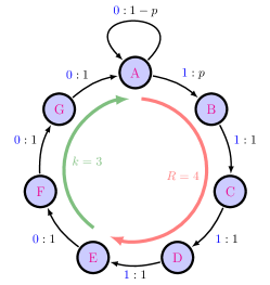
(a) $(4\text{-}3)$-GM Process of the $(R\text{-}k)$-Golden Mean family with $0\leq k=\nu_{0}(\zeta)\leq R=\nu_{0}(\mathcal{W})<\infty$, which generates processes with finite but tunable Markov-order $R$ and cryptic-order $k$.

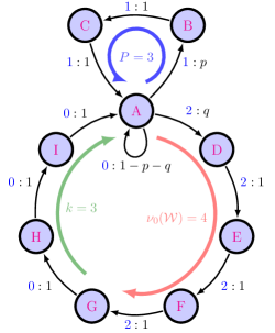
(b) $(4\text{-}3)$-GP-$(3)$ Process of the $(\nu_{0}(\mathcal{W})\text{-}k)$-Golden Parity-$(P)$ family with $0\leq k=\nu_{0}(\zeta)\leq\nu_{0}(\mathcal{W})<R=\infty$ whenever $P>1$, generates processes with infinite Markov-order $R$, tunable finite cryptic-order $k$, and tunable finite symmetry-collapse index $\nu_{0}(\mathcal{W})$.

(c) $(4\text{-}3)$-GPZ-$(3\text{-}3)$ Process of the $(\nu_{0}(\mathcal{W})\text{-}\nu_{0}(\zeta))$-Golden Parity-$(P\text{-}Z)$ family with $0\leq\nu_{0}(\zeta)\leq\nu_{0}(\mathcal{W})<k=R=\infty$ whenever $Z>1$. Markov order is infinite whenever either $P>1$ or $Z>1$. Cryptic-order is infinite when $Z>1$. This family generates processes with finite but tunable symmetry-collapse index $\nu_{0}(\mathcal{W})$ and cryptic index $\nu_{0}(\zeta)$.

Figure 2: Process families for exploring the roles of and interplay between Markov-order $R$, cryptic-order $k$, the symmetry-collapse index $\nu_{0}(\mathcal{W})$ of the zero eigenvalue of the synchronizing dynamic over mixed states, and the cryptic index $\nu_{0}(\zeta)$ of the zero eigenvalue of the cryptic operator presentation. We always have $k\leq R$ and $\nu_{0}(\zeta)\leq\nu_{0}(\mathcal{W})$. Whenever $\Lambda_{\mathcal{W}}=\Lambda_{T}\cup\{0\}$, $R$ is finite, $R=\nu_{0}(\mathcal{W})$ and $k=\nu_{0}(\zeta)$. Whenever $\Lambda_{\zeta}=\Lambda_{T}\cup\{0\}$, $k$ is finite, whether or not $R$ is, and $k=\nu_{0}(\zeta)$. When $k$ or $R$ is infinite, the cryptic index and symmetry-collapse index reveal more nuanced features of the cryptic and synchronization dynamics.

Coronal spectrograms demonstrate that complex systems behave according to the spectrum of their hidden linear dynamic. The relevant frequency-dependent measure $f(\omega)$ emanates from the nonzero eigenvalues of the hidden linear dynamic: the closer eigenvalues approach the unit circle, the sharper the observed peaks. At one extreme, one observes Bragg-like reflections (delta-function contributions) when the eigenvalues fall on the unit circle. The collection of diffuse peaks observed is a sum of Lorentzian-like and, what we might call, super-Lorentzian-like line profiles. Indeed, the Lorentzian-like line profiles are the discrete-time version of a Lorentzian curve. While the continuous-domain Lorentzian is given by $\text{Re}\bigl{(}\frac{c}{\omega-\lambda}\bigr{)}$, the continuous-to-discrete conformal mapping $\omega\to e^{i\omega}$ directly yields our discrete-domain analog $\text{Re}\bigl{(}\frac{c}{e^{i\omega}-\lambda}\bigr{)}$. The super-Lorentzian-like line profiles have the form $\text{Re}\bigl{[}(\frac{c}{e^{i\omega}-\lambda})^{n}\bigr{]}$.

Zero eigenvalues also contribute to $f(\omega)$, but only sinusoidal contributions of discrete increments from $\cos(\omega)$ up to $\cos(\nu_{0}\,\omega)$. Since these are qualitatively distinct from the super-Lorentzian contributions and do not emanate radially from the eigenvalues the same way contributions from nonzero eigenvalues do, coronal spectrograms are most useful for understanding the contributions of nonzero eigenvalues. Nevertheless, the two contributions can be usefully disentangled, as shown later.

We use both coronal spectrograms and coronated horizons to visualize various features in the examples to follow.

VI Examples

VI.1 Golden Mean Processes

To explore finite Markov order in relation to various complexity measures let’s consider the $(R\text{-}k)$-Golden Mean (GM) Processes . This process family describes a unique transition-parametrized process for each Markov-order $R\in\bigl{\{}\nu\in\mathbb{Z}:\nu\geq 1\bigr{\}}$ and each cryptic-order $k\in\bigl{\{}\kappa\in\mathbb{Z}:1\leq\kappa\leq R\bigr{\}}$. The $\epsilon$-machine for the $(4\text{-}3)$-Golden Mean Process is shown in Fig. 2a. From this the construction of all other $(R\text{-}k)$-Golden Mean processes can be discerned. In words, $(R\text{-}k)$-Golden Mean Processes are binary with alphabet $\mathcal{A}=\{{\color[rgb]{0,0,1}0},{\color[rgb]{0,0,1}1}\}$ and if the most recent history consists of at least $k$ consecutive ${\color[rgb]{0,0,1}0}$s (and no ${\color[rgb]{0,0,1}1}$s since then) then there is a probability $p$ of next observing a ${\color[rgb]{0,0,1}1}$ and a probability $1-p$ of simply seeing another ${\color[rgb]{0,0,1}0}$. This entails $R$ consecutive ${\color[rgb]{0,0,1}1}$s followed by at least $k$ consecutive ${\color[rgb]{0,0,1}0}$s.

The eigenvalues of the internal state-to-state transition matrix of the $\epsilon$-machine’s recurrent component are:

$$\Lambda_{T}=\Bigl{\{}\lambda\in\mathbb{C}:\bigl{(}\lambda-(1-p)\bigr{)}\lambda^{R+k-1}=p\Bigr{\}}~{}.$$

In the limit of $p\to 1$, all $(R\text{-}k)$-Golden Mean Processes become perfectly periodic. In this limit, the eigenvalues are evenly distributed on the unit circle:

$$\Lambda_{T}\to\bigl{\{}e^{in2\pi/(R+k)}\bigr{\}}_{n=0}^{R+k-1}~{}.$$

At the other extreme, as $p\to 0$, all eigenvalues evolve to zero, except the stationary eigenvalue at $z=1$. At any setting of $p$, the nonunity eigenvalues lie approximately on a circle within the complex plane whose radius decreases nonlinearly from $1$ to $0$ as $p$ is swept from $1$ to $0$. Simultaneously, this circle’s center moves from the origin to a positive real value and back to the origin as $p$ is swept from $1$ to $0$. Figure 3 shows how the eigenvalues of the $(5\text{-}3)$-Golden Mean Process evolve over the full range of $p$ as it sweeps from $1$ to $0$.

In contrast to the $p$-dependent spectrum of the recurrent structure just discussed, the only eigenvalue corresponding to the transient structure of the $\mathscr{S}$-MSP is equal to zero, regardless of the transition parameter $p$. Recall that this is necessarily true for any process with finite Markov order. Hence, $\Lambda_{\mathcal{W}}=\Lambda_{T}\cup\{0\}$, with $\nu_{0}(\mathcal{W})=R$. The cryptic structure is similar: $\Lambda_{\zeta}=\Lambda_{T}\cup\{0\}$, with $\nu_{0}(\zeta)=k$, where $\zeta$ is the state-to-state transition matrix of the cryptic operator presentation.

Table 1 compares the $\epsilon$-machines, autocorrelation, power spectra, MSPs, myopic entropy rates, and myopic state uncertainties for three $p$-parametrized examples of $(R\text{-}k)$-GM processes.

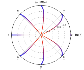
Figure 3: Evolution of eigenvalues $\Lambda_{T}$ of the recurrent component of the (5–3)-GM Process’s $\epsilon$-machine. Displayed within the unit circle of the complex plane, the trajectory of each eigenvalue follows a line that starts thick blue and ends thin red as the transition parameter $p$ evolves from $1$ to $0$. In addition to the seven eigenvalues that move from the nontrivial eighth roots of unity towards zero along nonlinear trajectories, the eigenvalue at $z=1$ does not change with $p$.

The autocorrelation of each process captures their ‘leaky periodic’ behaviors: The leakiness originates from the self-transition at state ${\color[rgb]{1,0,1}A}$ that adds a phase-slip noise to otherwise $(R+k)$–periodic behavior. Moreover, each process’ phase, and so its $\epsilon$-machine’s internal state, is uniquely identified after $R$ observations. This corresponds to the depth of the $\mathscr{S}$-MSP tree-like structure $\nu_{0}(\mathcal{W})=R$, the convergence of the myopic entropy rate $h_{\mu}(L)$ to the true entropy rate $h_{\mu}$ when conditioning on observations of finite block-length $L-1=R$, and the complete loss of causal state uncertainty $\mathcal{H}(L)$ after $L=R$ observations.

Table 1: Complexity analyses for finite Markov-order processes. Quantitative data used $p=1/2$.

A paradigm of finite Markov order, the $(5\text{-}3)$-Golden Mean Process has a strictly tree-like structure in its MSP’s transients, which have a maximum depth equal to both $\nu(\mathcal{W})$ and its Markov order of $5$.

These analyses illustrate the typical behaviors of complexity measures for finite Markov-order processes. We next investigate examples of infinite Markov-order processes to draw attention to the characteristic differences of nonzero eigenvalues in their MSP transient structures.

VI.2 Even Process

The Even Process, shown in the first column of Table 2, is a well known example of a stochastic process that cannot be generated by any finite Markov-order approximation, yet it is described by a simple two-state HMM.

Infinite Markov order, in this case, stems from the fact that the process generates only an even number of consecutive $1$s, between $0$s. The countably infinite set of Markov chain states necessary to track this parity reflects the infinite order. Moreover, the surplus entropy rate $h_{\mu}(L)-h_{\mu}$ incurred when using a finite order-$(L-1)$ Markov approximation vanishes only asymptotically, being the sum of decaying exponentials. (See Table 2.) This is in stark contrast to the myopic entropy rate for the finite Markov order processes of Table 1. For them $h_{\mu}(L)$ drops to $h_{\mu}$ exactly at $L=R+1$. Similarly, the average state uncertainty $\mathcal{H}(L)$ for infinite Markov processes converges only asymptotically—and with the same set of decay rates as $h_{\mu}(L)$—to its asymptotic value of $0$. (This curve is not shown in Table 2 for lack of space.) Such long-lived decay is driven by nonzero eigenvalues in the $\mathscr{S}$-MSP transient structure.

The Even Process is a relatively simple example of an infinite Markov-order process. As expected for infinite Markov-order, its MSP’s transient structure had nonzero eigenvalues. Generally, though, two ranges of contribution are to be expected in synchronization dynamics. The first is a finite-horizon contribution to the past-future mutual information, corresponding to completely ephemeral zero eigenvalues in the MSP’s transient structure. The second is an infinite-horizon contribution to the past–future mutual information, arising from nonzero eigencontributions.

Table 2: Complexity analyses for infinite Markov-order processes. Quantitative data used $p=1/2$ and $q=1/3$.

VI.3 Golden–Parity Process Family

To further explore the nature of infinite Markov order processes, we introduce the $(\nu_{0}\text{-}k)$-Golden-Parity-$(P)$ Processes. This family subsumes and extends the examples analyzed so far. The role of each parameter is explained in Fig. 2b, which displays a state-transition diagram of the $(4\text{-}3)$-GP-$(3)$ Process’ $\epsilon$-machine.

If $P=1$, the family reduces to the $(\nu_{0}\text{-}k)$-Golden Mean Process family, with tunable Markov $R=\nu_{0}(W)$ and cryptic $k$ orders. That is, $(\nu_{0}(\mathcal{W})\text{-}k)$-GP-$(1)$ = $(\nu_{0}(\mathcal{W})\text{-}k)$-GM. However, the Markov order becomes infinite whenever $P>1$. In this case the index $\nu_{0}(\mathcal{W})$ of the $\mathscr{S}$-MSP’s zero-eigenvalue—which controls the finite duration necessary to resolve all broken symmetries—and the cryptic order $k$ can still be tuned independently. The Even Process considered earlier is the $(0\text{-}0)$-Golden-Parity-$(2)$ Process.

Three examples of $(\nu_{0}(\mathcal{W})\text{-}k)$-Golden-Parity-$(P)$ processes are analyzed in Table 2. The $\mathscr{S}$-MSP transient structure for the second two clarifies the difference between (i) the symmetry collapse associated with completely ephemeral transient states that are fully depleted of probability density after $\nu_{0}(\mathcal{W})$ time-steps and (ii) the long-lived leaky transients whose probability density only vanishes as more-refined ambiguity is resolved.

Examining the myopic entropy convergence $h_{\mu}(L)$, the effect of these distinct routes to synchronization on the predictability can be seen: The process is much more predictable, on average, after $\nu_{0}(\mathcal{W})$ time-steps. However, the average predictability of an infinite-Markov-order process continues to increase with increasing observation window, albeit with exponentially diminishing returns. In general, we showed that this asymptotic convergence occurs as a sum of decaying exponentials from diagonalizable subspaces and as the product of polynomials and exponentials in the case of nondiagonalizable structures associated with nonzero eigenvalues. The apparent oscillations under the exponential decays are completely described by the leaky periodicities of the eigenvalues in the transient belief states.

Finally, note that the excess entropy spectrum $\mathcal{E}(\omega)$ shows the frequency domain view of observation-induced predictability. ${\bf E}=\lim_{\omega\to 0}\mathcal{E}(\omega)$ is the total past–future mutual information, which is also the excess entropy observed before full synchronization. The $\nu_{0}(\mathcal{W})$ symmetry collapse contributes significantly and early to the total excess entropy of the last two examples. Whereas, the asymptotic tails of synchronization associated with leaky periodicity of particular transient states of uncertainty accumulate their contribution to excess entropy rather slowly.

In addition to new intuitions about convergence behaviors in stochastic processes, the general and broadly applicable theoretical results here allow novel numerical investigations and unprecedentedly-accurate analyses of infinite-Markov-order processes. As an example of the latter, let us summarize several of the exact results derived in App. A for the $(p,q)$-parametrized $(2\text{-}1)$-GP-$(2)$ process explored in Table 2’s second column.

Depending on whether the transition parameter $p$ is larger or smaller than $2\sqrt{q}-q$, App. A found qualitatively distinct behaviors dominate the $(2\text{-}1)$-GP-$(2)$ process. This hints at a general principle: behaviorally distinct regions are separated by a critical line in the $(p,q)$-parameter space along which the transition dynamic $T$ becomes nondiagonalizable. For $p<2\sqrt{q}-q$, the autocorrelation for $|L|\geq 2$ has the exact solution:

$$\gamma(L) =\beta^{2}+\beta\,q^{|L|/2}\,\text{Re}\bigl{(}\zeta\,e^{i\omega_{\xi}|L|}\bigr{)}~{},$$ (37)

where $\beta\equiv 2(p+2q)/(1+p+2q)$, $\zeta\equiv(\xi+1)^{2}(p\xi+2q)/(\xi(\xi^{3}+p\xi+2q))$, $\xi\equiv-\frac{1}{2}(p+q)+i\frac{1}{2}\sqrt{4q-(p+q)^{2}}$, and $\omega_{\xi}\equiv\tfrac{\pi}{2}+\arctan\bigl{(}(p+q)/\sqrt{4q-(p+q)^{2}}\bigr{)}$. The corresponding power spectrum is:

$$P(\omega) =\frac{8q}{1+p+2q}+\frac{2p}{1+p+2q}\bigl{[}1-\cos(\omega)\bigr{]}$$

$$\qquad+\beta\,\text{Re}\Bigl{(}\frac{\zeta\xi}{e^{i\omega}-\xi}+\frac{\zeta\xi}{e^{-i\omega}-\xi}\Bigr{)}$$

$$\qquad+2\pi\beta^{2}\sum_{k=-\infty}^{\infty}\delta(\omega+2\pi k)~{}.$$ (38)

For any parameter setting, the metadynamic of observation-induced synchronization to the $(2\text{-}1)$-GP-$(2)$ process is nondiagonalizable due to the index-$2$ zero eigenvalue. This leads to a completely ephemeral contribution to $h_{\mu}(L)$ up to $L=2$. For $L\geq 3$, we find the myopic entropy rate relaxes asymptotically to the true entropy rate according to:

$$h_{\mu}(L)-h_{\mu} =\begin{cases}\frac{-p\log p+(1+p)\log(1+p)-2p}{\sqrt{p}(1+p+2q)}\,p^{L/2}&\text{for odd }L,\\ \frac{p\log p-(1+p)\log(1+p)+2}{(1+p+2q)}\,p^{L/2}&\text{for even }L,\end{cases}$$

where the process’ true entropy rate is:

$$h_{\mu} =\frac{-q\log q-p\log p-(1-p-q)\log(1-p-q)}{1+p+2q}~{}.$$

Interestingly, while the autocorrelation at separation $L$ scales as $\sim q^{L/2}$, the predictability of single-symbol transitions between slightly shifted histories of length $L$ converges as $\sim p^{L/2}$—indicating two rather independent decay rates.

The amount of the future that can be predicted from the past is the total mutual information between the observable past and observable future:

$${\bf E} =\tfrac{(1-p-q)\log(1-p-q)-p\log p-q\log q-(1-p)\log(1-p)}{1+p+2q}$$

$$\qquad+\log(1+p+2q)~{}.$$

However, to actually perform prediction requires more memory than this amount of shared information. Calculation of additional measures and more detail can be found in App. A.

To explore the structure in infinite-cryptic order processes, one can use the more generalized family of $(\nu_{0}(\mathcal{W})\text{-}\nu_{0}(\zeta))$-GP-$(P\text{-}Z)$ Processes. For them, $\nu_{0}(\zeta)$ is the index of the zero-eigenvalue of the cryptic operator presentation and the process has infinite cryptic order whenever $Z>1$. Above, $Z=1$ and $(\nu_{0}(\mathcal{W})\text{-}\nu_{0}(\zeta))$-GP-$(P\text{-}1)$ = $(\nu_{0}(\mathcal{W})\text{-}\nu_{0}(\zeta))$-GP-$(P)$. Since the preceding examples served well enough to illustrate the power of spectral decomposition, our main goal, we leave a full analysis of this family to interested others.

VII Predicting Superpairwise Structure

The Random–Random–XOR (RRXOR) Process is generated by a simple HMM. Figure 4 displays its five-state $\epsilon$-machine. However, it illustrates nontrivial, counterintuitive features typical of stochastic dynamic information processing systems. The process is defined over three steps that repeat: (i) a $\color[rgb]{0,0,1}0$ or $\color[rgb]{0,0,1}1$ is output with equal probability, (ii) another $\color[rgb]{0,0,1}0$ or $\color[rgb]{0,0,1}1$ is output with equal probability, and then (iii) the eXclusive-OR operation (XOR) of the last two outputs is output.

Figure 4: RRXOR Process $\epsilon$-machine.

Surprisingly, but calculations easily verify, there are no pairwise correlations. All of its correlations are higher than second order. One consequence is that its power spectrum is completely flat—the signature of white noise; see Fig. 5. This would lead a casual observer to incorrectly conclude that the generated time series has no structure. In fact, a white noise spectrum is an indication that, if structure it present, it must be hidden in higher-order correlations.

The RRXOR Process clearly is not structureless—via the exclusive OR, it transforms information in a substantial way. We show that the complexity measures introduced above can detect this higher-order structure. However, let us first briefly consider why the correlation-based measures fail to detect structure in the RRXOR Process.

It is sometimes noted that information measures are superior to standard measures of correlation since they capture nonlinear dependencies, while the standard correlation relies on linear models. And so, we can avoid this problem by using the information correlation $\operatorname{I}[X_{0};X_{\tau}]$ rather than autocorrelation. Analogous to autocorrelation, it too has a spectral version—the power-of-pairwise information (POPI) spectrum:

$$\mathcal{I}(\omega)\equiv-\operatorname{H}(X_{0})+\lim_{N\to\infty}\sum_{\tau=-N}^{N}e^{-i\omega\tau}\operatorname{I}[X_{0};X_{\tau}]~{}.$$ (39)

It is easy to show that $\mathcal{I}(\omega)=0$ for the RRXOR Process. Hence, as Fig. 5 showed, such measures are not sufficient to detect even simple computational structure, since they only can detect pairwise statistical dependencies.

In stark contrast, the excess entropy spectrum $\mathcal{E}(\omega)$ does identify the structure of hidden dependencies in the RRXOR Process; see Fig. 6. Why? The brief detour through power spectra, information correlation, and POPI spectra brings us to a deeper understanding of why $\mathcal{E}(\omega)$ is successful at detecting nuanced computational structure in a time series. Since it partitions all random variables throughout time, the excess entropy itself picks up any systematic influence the past has on the future. The excess entropy spectrum further identifies the frequency decomposition of any such linear or nonlinear dependencies. In short, all multivariate dependencies contribute to the excess entropy spectrum.

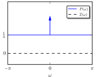
Figure 5: Power spectrum $P(\omega)$ and POPI spectrum $\mathcal{I}(\omega)$ of the RRXOR Process: The first is flat and the second identically zero. One might incorrectly conclude the RRXOR Process is structureless white noise.

\begin{overpic}[width=199.4681pt,unit=1mm]{img/RRX_coronated_horizon.pdf} \put(58.0,60.0){\includegraphics[width=43.36464pt]{img/EE_legend_fully_annotated.pdf}} \put(-1.0,20.0){\rotatebox{90.0}{$|\lambda|$}} \put(42.5,1.0){\scalebox{1.1}{$\omega$}} \end{overpic}

Figure 6: Excess entropy spectrum of the RRXOR Process, together with the eigenvalues of the $\mathscr{S}$-MSP transition matrix $\mathcal{W}$. Among the power spectrum, POPI spectrum, and excess entropy spectrum, only the excess entropy spectrum is able to detect structure in the RRXOR Process since the structure is beyond pairwise. The eigenspectrum of the MSP of the RRXOR $\epsilon$-machine and the excess entropy spectrum both indicate that the RRXOR Process is indeed structured, with both ephemeral symmetry breaking and leaky periodicities in the convergence to optimal predictability.

Let us now consider the hidden structure of the RRXOR Process in more detail. With reference to Fig. 4, we observe that the expected probability density over causal states evolves through the $\epsilon$-machine with a period-$3$ modulation. In a given realization, the particular symbols emitted after each phase resetting ($\phi=0$) break symmetries with respect to which “wings” of the $\epsilon$-machine structure are traversed. This is reflected in $T$’s eigenvalues: the three roots of unity $\{e^{in2\pi/3}\}_{n=0}^{2}$ and two zero eigenvalues, with $a_{0}(T)=g_{0}(T)=2$ giving index $\nu_{0}(T)=1$.

The period-$3$ modulation leads to a phase ambiguity when an observer synchronizes to the process, an ambiguity that resolved in the MSP transient structure. This resolution is rather complicated, as made explicit in the RRXOR Process’ $\mathscr{S}$-MSP, shown in Fig. 7. There are $31$ transient states of uncertainty, in addition to the five recurrent states—$36$ causal states in total.

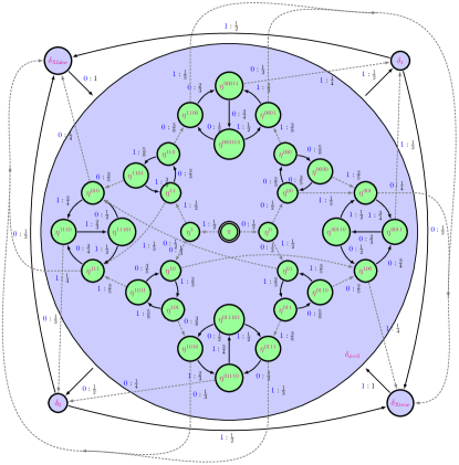
Figure 7: MSP of the RRXOR Process’ $\epsilon$-machine: Grayed out (and dashed) transitions permanently leave the states from which they came. Recognizing the manner by which these transitions partition the mixed-state space allows simplified spectrum calculations. The directed graph structure is inherently nonplanar. The large blue recurrent state should be visualized as being behind the transient states; it does not contain them.

Since we derived the $\epsilon$-machine’s $\mathscr{S}$-MSP, $W=\mathcal{W}$. Hence, the MSP’s layout depicts the information processing involved while an observer synchronizes to the RRXOR Process. This graphically demonstrates the burden on an optimal predictor, even one that only needs to learn an average of $h_{\mu}$ bits per observation to optimally predict the process.

The MSP introduces new, relevant zero eigenvalues associated with its transient states. In particular, the first-encountered tree-like transients (starting with mixed-state $\pi$) introduce new Jordan blocks up to dimension $2$. Overall, the $0$-eigenspace of $W$ has index $2$, so that $\nu_{0}(W)=2$.

Two different sets of leaky-period-$3$ structures appear in the MSP transients. There are four leaky three-state cycles, each with the same leaky-period-3 contributions to the spectrum: $\bigl{\{}(\tfrac{1}{4})^{1/3}e^{in2\pi/3}\bigr{\}}_{n=0}^{2}$. There are also four leaky four-state cycles, each with a leaky-period-3 contribution and symmetry-breaking 0-eigenvalue contribution to the spectrum: $\bigl{\{}(\tfrac{1}{2})^{1/3}e^{in2\pi/3}\bigr{\}}_{n=0}^{2}\cup\{0\}$. The difference in eigenvalue magnitude, $(\tfrac{1}{4})^{1/3}$ versus $(\tfrac{1}{2})^{1/3}$, implies different timescales of synchronization associated with distinct learning tasks. For example, an immediate lesson is that it takes longer (on average) to escape the $4$-state leaky-period-$3$ components (from the time of arrival) than to escape the preceding $3$-state leaky-period-$3$ components of the synchronizing metadynamic.

\begin{overpic}[width=216.81pt,unit=1mm]{img/hmuL.pdf} \put(67.0,50.5){\scalebox{0.85}{$h_{\multimap}\!+h_{\rightsquigarrow}$}} \put(70.0,46.5){\scalebox{0.85}{$h_{\rightsquigarrow}$}} \end{overpic}

Figure 8: Ephemeral ($h_{\multimap}(L)$) and persistent ($h_{\rightsquigarrow}(L)$) contributions to the myopic entropy rate ($h_{\mu}(L)$). The ephemeral contribution lasts only up to $L=\nu_{0}(W)=2$.

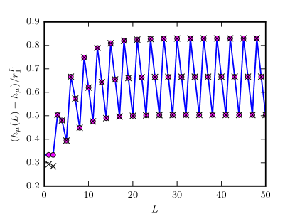
Figure 9: Tails of the myopic entropy convergence $h_{\mu}(L)$ shown in Fig.  8 decay according to two different leaky period-three envelopes. The latter correspond to the two qualitatively different types of transient synchronization cycles in the MSP of Fig. 7. One of the transient cycles has a relatively fast decay rate of $r_{2}=(1/4)^{1/3}$. While the slower decay rate of $r_{1}=(1/2)^{1/3}$ dominates $h_{\mu}(L)$’s deviation from $h_{\mu}$ at large $L$.

The entropy rate convergence plots of Figs. 8 and 9 reveal a sophisticated predictability modulation that simply could not have been gleaned from the spectra of Fig. 5. Figure 9 emphasizes the dominance of the slowest-decaying eigenmodes for large $L$. Such oscillations under the exponential convergence to synchronization are typical. However, as seen in comparison with Fig. 8 much of the uncertainty may be reduced before this asymptotic mode comes to dominate. Ultimately, synchronization to optimal prediction may involve important contributions from all modes of the mixed-state-to-state metadynamic.

This detailed analysis of the RRXOR Process suggests several general lessons about how we view information in stochastic processes. First, as information processing increases in sophistication, a vanishing amount of a process’ intrinsic structure will be discernible at low-orders of correlation. Second, logical computation, as implemented by universal logic gates, primarily operates above pairwise correlation. And so, finally, there is substantial motivation to move beyond measures of pairwise correlation. We must learn to recognize hidden structures and to use higher-order structural investigations to better understand information processing. This is critical to empirically probing functionality in biological and engineered processes.

VIII Conclusion

Surprisingly, many questions we ask about structured stochastic, nonlinear processes implicate a linear dynamic over an appropriate hidden state space. That is, there is an implied hidden Markov model. The promise is that once the dynamic is found for the question of interest, one can make progress in analyzing it. Unfortunately, a roadblock immediately arises: these hidden linear dynamics are generically nondiagonalizable for questions related to prediction and to information and complexity measures. Deploying Part I’s meromorphic functional calculus, though, circumvents the roadblock. Using it, we determined closed-form expressions for a very wide range of information and complexity measures. Often, these expressions turned out to be direct functions of the HMM’s transition dynamic.

This allowed us to catalog in detail the range of possible convergence behaviors for correlation and myopic uncertainty. We then considered complexity measures that accumulate during the transient relaxation to observer synchronization. We also introduced the new notion of complexity spectra, gave a new kind of information-theoretic signal analysis in terms of coronal spectrograms, and highlighted common simplifications for special cases, such as almost diagonalizable dynamics. We closed by analyzing several families of finite and infinite Markov and cryptic order processes and emphasized the importance of higher-than-pairwise-order correlations, showing how the excess entropy spectrum is the key diagnostic tool for them.

The analytical completeness might suggest that we have reached an end. Partly, but the truth we seek is rather farther down the road. The meromorphic functional calculus of nondiagonalizable operators merely sets the stage for the next challenges—to develop complexity measures and structural decompositions for infinite-state and infinite excess entropy processes. Hopefully, the new toolset will help us scale the hierarchies of truly complex processes outlined in Refs. [5, 4, 1], at a minimum giving exact answers at each stage of a convergent series of finite-$\epsilon$-machine approximations.

Appendix A Example Analytical Calculations

To exercise the operational nature of the framework introduced, the following explicitly carries out the analytic calculations to obtain the closed-form complexity measures for the $(p,q)$-parametrized $(2\text{-}1)$-GP-$(2)$ Process. This process was already visually explored in the second column of Table 2. And so, the goal here is primarily pedagogical—providing insight and better explicating particular calculational steps. The appendix demonstrates a variety of techniques in the spirit of a tutorial, though many were not called out in the main development.

A.1 Process and spectra features

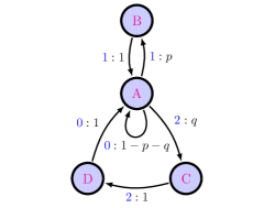
Figure 10: $\epsilon$-Machine of the $(2\text{-}1)$-GP-$(2)$ Process.

The $(p,q)$-parametrized $(2\text{-}1)$-GP-$(2)$ Process is described by its $\epsilon$-machine, whose state-transition diagram was shown in the first row and second column of Table 2 and is reproduced here in Fig. 10. Formally, the $(2\text{-}1)$-GP-$(2)$ stationary stochastic process is generated by the HMM $\mathcal{M}_{\epsilon\text{M}}=\bigl{(}\bm{\mathcal{S}},\mathcal{A},\{T^{({x})}\}_{{x}\in\mathcal{A}},\eta_{0}=\pi\bigr{)}$. That is, $\mathcal{M}$ consists of a set of hidden causal states $\bm{\mathcal{S}}=\{{\color[rgb]{1,0,1}\text{A}},{\color[rgb]{1,0,1}\text{B}},{\color[rgb]{1,0,1}\text{C}},{\color[rgb]{1,0,1}\text{D}}\}$, an alphabet $\mathcal{A}=\{{\color[rgb]{0,0,1}0},{\color[rgb]{0,0,1}1},{\color[rgb]{0,0,1}2}\}$ of symbols emitted to form the observed process, and a set $\bigl{\{}T^{({x})}:T^{({x})}_{s,s^{\prime}}=\Pr(X_{t}={x},\mathcal{S}_{t+1}=s^{\prime}|\mathcal{S}_{t}=s)\bigr{\}}_{{x}\in\mathcal{A}}$ of symbol-labeled transition matrices. These are:

$$T^{(0)} =\begin{bmatrix}\scalebox{0.75}{$1\!-\!p\!-\!q$}&0&0&0\\ 0&0&0&0\\ 0&0&0&0\\ 1&0&0&0\\ \end{bmatrix}~{},$$

$$T^{(1)} =\begin{bmatrix}\;0\;&p\,&0\,&0\;\\ \;1&0&0&0\\ \;0&0&0&0\\ \;0&0&0&0\\ \end{bmatrix}~{},$$

and

$$T^{(2)} =\begin{bmatrix}\;0\;&0\,&q\,&0\;\\ \;0&0&0&0\\ \;0&0&0&1\\ \;0&0&0&0\\ \end{bmatrix}~{}.$$

The symbol-labeled transition matrices sum to the row-stochastic internal state-to-state transition matrix:

$$T=\sum_{{x}\in\mathcal{A}}T^{({x})}=\begin{bmatrix}\scalebox{0.75}{$1\!-\!p\!-\!q$}&p&q&0\\ 1&0&0&0\\ 0&0&0&1\\ 1&0&0&0\\ \end{bmatrix}~{}.$$

This is a Markov chain over the hidden states. From it we find the stationary state distribution $\bra{\pi}=\bra{\pi}T$:

$$\bra{\pi}=\frac{1}{1+p+2q}\begin{bmatrix}1&p&q&q\end{bmatrix}~{}.$$

The first analysis task is to determine the eigenvalues and associated projection operators for the internal state-to-state transition matrix $T$. From:

$$\det(T-\lambda I) =\lambda(\lambda-1)\bigl{(}\lambda^{2}+(p+q)\lambda+q\bigr{)}$$

$$=0~{},$$

we find the four eigenvalues:

$$\Lambda_{T}=\bigl{\{}1,\,0,\,-\tfrac{1}{2}(p+q)\pm\tfrac{1}{2}\sqrt{(p+q)^{2}-4q}\,\bigr{\}}~{}.$$

All eigenvalues are real for $p\geq 2\sqrt{q}-q$. Two are complex with nonzero imaginary part when $p<2\sqrt{q}-q$. Putting this together with the transition-probability consistency constraint that $p+q<1$ yields the map of the transition-parameter space shown in Fig. 11.

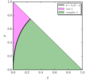
Figure 11: Transition-probability space for the $(p,q)$-parametrized $(2\text{-}1)$-GP-$(2)$ Process.

For a generic choice of the parameter setting $(p,q)$, all $T$’s eigenvalues are unique, and so $T$ is diagonalizable. However, two of the eigenvalues become degenerate along the parameter subspace $p=2\sqrt{q}-q$, giving $\Lambda_{T}=\{1,0,-\sqrt{q}\}$. We find that the algebraic multiplicity $a_{-\sqrt{q}}=2$ is larger than the geometric multiplicity $g_{-\sqrt{q}}=1$, yielding nondiagonalizability ($\nu_{-\sqrt{q}}=2$) along this ($p=2\sqrt{q}-q$)-submanifold. More broadly, experience has shown that eigenvalues generically induce nondiagonalizability when they collide and scatter in the complex plane. For example, this occurs when a pair of eigenvalues first “entangle” to become complex conjugate pairs.

For any parameter setting ($p,q$), we find $T$’s right eigenvectors from $(T-\lambda I)\ket{\lambda}=\ket{0}$. They are:

$$\ket{0} =\begin{bmatrix}0&1&-p/q&0\end{bmatrix}^{\top}$$

and

$$\ket{\lambda} =\begin{bmatrix}\lambda^{2}&\lambda&1&\lambda\end{bmatrix}^{\top}~{},$$

for all $\lambda\in\Lambda_{T}\setminus\{0\}$. Similarly, we find the left eigenvectors of $T$ from $\bra{\lambda}(T-\lambda I)=\ket{0}$:

$$\bra{0} =\begin{bmatrix}0&1&0&-1\end{bmatrix}$$

and

$$\bra{\lambda} =\begin{bmatrix}\lambda^{2}&p\lambda&q\lambda&q\end{bmatrix}~{},$$

for all $\lambda\in\Lambda_{T}\setminus\{0\}$. Clearly, the left eigenvectors are not simply the complex-conjugate transpose of the right eigenvectors. This is a signature of the more intricate algebraic structure in these processes.

Since $T$ is generically diagonalizable, all of the projection operators are simply the normalized ket-bra outer products:

$$T_{\lambda}=\frac{\ket{\lambda}\bra{\lambda}}{\braket{\lambda}{\lambda}}~{},$$

so long as $p\neq 2\sqrt{q}-q$. To wit:

$$T_{1} =\frac{\ket{1}\bra{1}}{\braket{1}{1}}$$

$$=\ket{\mathbf{1}}\bra{\pi}~{}.$$

Along the nondiagonalizable ($p=2\sqrt{q}-q$)-subspace of parameter settings: $\braket{{}^{-}\sqrt{q}}{{}^{-}\sqrt{q}}=0$. This corresponds to the fact that the right and left eigenvectors are now dual to the left and right generalized eigenvectors, rather than being dual to each other. We find the projection operator for the nondiagonalizable eigenspace is:

$$T_{-\sqrt{q}}=\frac{\ket{{}^{-}\sqrt{q}^{(1)}}\bra{{}^{-}\sqrt{q}^{(2)}}}{\braket{{}^{-}\sqrt{q}^{(2)}}{{}^{-}\sqrt{q}^{(1)}}}+\frac{\ket{{}^{-}\sqrt{q}^{(2)}}\bra{{}^{-}\sqrt{q}^{(1)}}}{\braket{{}^{-}\sqrt{q}^{(1)}}{{}^{-}\sqrt{q}^{(2)}}}~{},$$

where:

$$\ket{{}^{-}\sqrt{q}^{(1)}} =\begin{bmatrix}q&-\sqrt{q}&\;1&-\sqrt{q}\end{bmatrix}^{\top}~{},$$

$$\ket{{}^{-}\sqrt{q}^{(2)}} =\begin{bmatrix}-\sqrt{q}&0&1/\sqrt{q}&0\end{bmatrix}^{\top}~{},$$

$$\bra{{}^{-}\sqrt{q}^{(1)}} =\begin{bmatrix}q&q(\sqrt{q}-2)&-q\sqrt{q}&q\end{bmatrix}~{},\text{ and}$$

$$\bra{{}^{-}\sqrt{q}^{(2)}} =\begin{bmatrix}-\sqrt{q}&0&0&\sqrt{q}\end{bmatrix}~{}.$$

Equivalently, $T_{-\sqrt{q}}=I-T_{1}-T_{0}$. The projection operators for the remaining ($\lambda=0,1$) eigenspaces retain the same form as before: $T_{\lambda}=\ket{\lambda}\bra{\lambda}/\braket{\lambda}{\lambda}$.

A.2 Observed correlation

The pieces are now in place to calculate the observable correlation and power spectrum. Recall that we derived the general spectral decomposition of the autocorrelation function $\gamma(L)=\left\langle\overline{{X}}_{t}{X}_{t+L}\right\rangle_{t}$:

$$\gamma(L) =\sum_{\lambda\in\Lambda_{T}\atop\lambda\neq 0}\sum_{m=0}^{\nu_{\lambda}-1}\bra{\pi\overline{\mathcal{A}}}T_{\lambda,m}\ket{\mathcal{A}\mathbf{1}}\binom{|L|-1}{m}\lambda^{|L|-1-m}$$

$$\qquad+[0\in\Lambda_{T}]\sum_{m=0}^{\nu_{0}-1}\bra{\pi\overline{\mathcal{A}}}T_{0}T^{m}\ket{\mathcal{A}\mathbf{1}}\delta_{|L|-1,m}$$

for nonzero integer $L$, where:

$$\bra{\pi\overline{\mathcal{A}}} =\bra{\pi}\sum_{{x}\in\mathcal{A}}\overline{{x}}T^{({x})}$$

$$=\frac{1}{1+p+2q}\begin{bmatrix}p&p&2q&2q\end{bmatrix}~{},$$

and:

$$\ket{\mathcal{A}\mathbf{1}} =\sum_{{x}\in\mathcal{A}}{x}T^{({x})}\ket{\mathbf{1}}$$

$$=\begin{bmatrix}p+2q&1&2&0\end{bmatrix}^{\top}~{}.$$

For generic parameter settings, this reduces to:

$$\gamma(L) =\frac{\bra{\pi\overline{\mathcal{A}}}0\rangle\langle 0\ket{\mathcal{A}\mathbf{1}}}{\braket{0}{0}}\delta_{|L|,1}$$

$$\qquad+\sum_{\lambda\in\Lambda_{T}\atop\lambda\neq 0}\frac{\bra{\pi\overline{\mathcal{A}}}\lambda\rangle\langle\lambda\ket{\mathcal{A}\mathbf{1}}}{\braket{\lambda}{\lambda}}\lambda^{|L|-1}$$

$$=4\left(\frac{p+2q}{1+p+2q}\right)^{2}+\frac{-p}{1+p+2q}\delta_{|L|,1}$$

$$\qquad+\frac{p+2q}{1+p+2q}\sum_{\lambda\in\Lambda_{T}\atop\lambda\neq 0,1}\frac{(\lambda+1)^{2}(p\lambda+2q)}{\lambda^{3}+p\lambda+2q}\lambda^{|L|-1}~{}.$$

Notably, the autocorrelation splits into an ephemeral part (via the Kronecker delta) due to the zero eigenvalue, an exponentially decaying oscillatory part due to the two eigenvalues with magnitude between $0$ and $1$, and an asymptotic part that survives even as $L\to\infty$ due to the eigenvalue of unity. Moreover, for $p<2\sqrt{q}-q$, the two nontrivial eigenvalues become complex conjugate pairs. This allows us to rewrite the autocorrelation for the $(2\text{-})$-GP-$(2)$ process for $|L|\geq 2$ concisely as:

$$\gamma(L) =\beta^{2}+\beta\,q^{|L|/2}\,\text{Re}\bigl{(}\zeta\,e^{i\omega_{\xi}|L|}\bigr{)}~{},$$

where:

$$\beta \equiv\frac{2(p+2q)}{1+p+2q}~{},$$

$$\zeta \equiv\frac{(\xi+1)^{2}(p\xi+2q)}{\xi(\xi^{3}+p\xi+2q)}~{},$$

$$\xi \equiv-\frac{1}{2}(p+q)+i\frac{1}{2}\sqrt{4q-(p+q)^{2}}~{},\text{ and}$$

$$\omega_{\xi} \equiv\frac{\pi}{2}+\arctan\bigl{(}\frac{p+q}{\sqrt{4q-(p+q)^{2}}}\bigr{)}~{}.$$

The latter form reveals that the magnitude of the largest nonunity eigenvalue $|\xi|=\sqrt{q}$ controls the slowest rate of decay of observed correlation $|\gamma(L)|\sim\sqrt{q}^{L}$ and that the complex phase of the eigenvalues determine the oscillations within this exponentially decaying envelope.

We found the general spectral decomposition of the continuous part of the power spectrum is:

$$P_{\text{c}}(\omega) =\bigl{\langle}\left|x\right|^{2}\bigr{\rangle}+2\sum_{\lambda\in\Lambda_{T}}\sum_{m=0}^{\nu_{\lambda}-1}\,\text{Re}\,\frac{\bra{\pi\overline{\mathcal{A}}}T_{\lambda,m}\ket{\mathcal{A}\mathbf{1}}}{(e^{i\omega}-\lambda)^{m+1}}~{}.$$

Also, recall from earlier that the delta functions of the power spectrum arise from $T$’s eigenvalues that lie on the unit circle:

$$P_{\text{d}}(\omega) =\sum_{k=-\infty}^{\infty}\sum_{\lambda\in\Lambda_{T}\atop|\lambda|=1}2\pi\,\delta(\omega-\omega_{\lambda}+2\pi k)$$

$$\qquad\qquad\qquad\times\text{Re}\bigl{(}\lambda^{-1}\bra{\pi\overline{\mathcal{A}}}\,T_{\lambda}\ket{\mathcal{A}\mathbf{1}}\bigr{)}~{},$$

where $\omega_{\lambda}$ is related to $\lambda$ by $\lambda=e^{i\omega_{\lambda}}$. As long as $p+q<1$, $\lambda=1$ is the only eigenvalue that lies on the unit circle, so that:

$$P_{\text{d}}(\omega)=\sum_{k=-\infty}^{\infty}2\pi\,\delta(\omega+2\pi k)\text{Re}\bra{\pi\overline{\mathcal{A}}}\,T_{1}\ket{\mathcal{A}\mathbf{1}}~{},$$

with:

$$\text{Re}\bra{\pi\overline{\mathcal{A}}}\,T_{1}\ket{\mathcal{A}\mathbf{1}} =\beta^{2}$$

$$=4\left(\frac{p+2q}{1+p+2q}\right)^{2}~{}.$$

Putting this all together we find the complete power spectrum for the $(2\text{-}1)$-GP-$(2)$ Process:

$$P(\omega) =\frac{8q}{1+p+2q}+\frac{2p}{1+p+2q}\bigl{[}1-\cos(\omega)\bigr{]}$$

$$\qquad+\beta\sum_{\lambda\in\Lambda_{T}\atop\lambda\neq 0,1}\text{Re}\left(\frac{(\lambda+1)^{2}(p\lambda+2q)}{\lambda^{3}+p\lambda+2q}\cdot\frac{1}{e^{i\omega}-\lambda}\right)$$

$$\qquad+2\pi\beta^{2}\sum_{k=-\infty}^{\infty}\delta(\omega+2\pi k)~{},$$

Thus, the process exhibits delta functions from the eigenvalue on the unit circle, continuous Lorentzian-like line profiles emanating from finite eigenvalues inside the unit circle which express the process’ chaotic nature, and the unique sinusoidal contribution that can only come from zero eigenvalues.

Whenever $p<2\sqrt{q}-q$, the two nontrivial eigenvalues become complex conjugate pairs. This allows us to rewrite the process’ power spectrum in a more transparent way:

$$P(\omega) =\frac{8q}{1+p+2q}+\frac{2p}{1+p+2q}\bigl{[}1-\cos(\omega)\bigr{]}$$

$$\qquad+\beta\,\text{Re}\left(\frac{\zeta\xi}{e^{i\omega}-\xi}+\frac{\zeta\xi}{e^{-i\omega}-\xi}\right)$$

$$\qquad+2\pi\beta^{2}\sum_{k=-\infty}^{\infty}\delta(\omega+2\pi k)~{},$$

which is clearly symmetric about $\omega=0$.

The level of completeness achieved is notable: we calculated these properties exactly in closed form for this infinite-Markov order stochastic process over the full range of possible parameter settings. Moreover, once it constructs the process’ $\mathscr{S}$-MSP, the next section goes on to produce the same level of analytical completeness but for predictability.

A.3 Predictability

To analyze the process’ predictability, we need the $\mathscr{S}$-MSP of any of its generators. Since we started already with the $\epsilon$-machine, we directly determine its $\mathscr{S}$-MSP. This gives the mixed-state transition matrix $W=\mathcal{W}$ that, in turn, suffices for calculating both predictability in this section and the synchronization necessary for prediction in the next.

We construct the $\mathscr{S}$-MSP by calculating all mixed states that can be induced by observation from the start distribution $\pi$ and then calculating the transition probabilities between them. There are eight such mixed-state distributions over $\bm{\mathcal{S}}$. However, four of them (${\color[rgb]{1,0,1}\delta_{\text{A}}}$, ${\color[rgb]{1,0,1}\delta_{\text{B}}}$, ${\color[rgb]{1,0,1}\delta_{\text{C}}}$, and ${\color[rgb]{1,0,1}\delta_{\text{D}}}$) correspond to completely synchronized peaked distributions. The other four states are new (relative to the recurrent states) transient states and correspond to transient states of recurrent-state uncertainty during synchronization. Calculating, we find the eight unique mixed-state distributions iteratively from:

$$\bra{\eta^{wx}}=\frac{\bra{\eta^{w}}T^{(x)}}{\bra{\eta^{w}}T^{(x)}\ket{\mathbf{1}}}~{},$$

starting with:

$$\bra{\eta^{x}}=\frac{\bra{\pi}T^{(x)}}{\bra{\pi}T^{(x)}\ket{\mathbf{1}}}~{},$$

are:

$$\bra{\pi} =\frac{1}{1+p+2q}\begin{bmatrix}1&p&q&q\end{bmatrix}~{},$$

$$\bra{\eta^{1}} =\frac{1}{2}\begin{bmatrix}1&1&0&0\end{bmatrix}~{},$$

$$\bra{\eta^{11}} =\frac{1}{1+p}\begin{bmatrix}1&p&0&0\end{bmatrix}~{},$$

$$\bra{\eta^{2}} =\frac{1}{2}\begin{bmatrix}0&0&1&1\end{bmatrix}~{},$$

$$\bra{\delta_{\text{A}}} =\begin{bmatrix}1&0&0&0\end{bmatrix}~{},$$

$$\bra{\delta_{\text{B}}} =\begin{bmatrix}0&1&0&0\end{bmatrix}~{},$$

$$\bra{\delta_{\text{C}}} =\begin{bmatrix}0&0&1&0\end{bmatrix}~{},\text{ and}$$

$$\bra{\delta_{\text{D}}} =\begin{bmatrix}0&0&0&1\end{bmatrix}~{}.$$

In this, the transient mixed states $\eta^{w}$ are labeled according to the shortest word $w$ that induces them. These distributions constitute the set of mixed-states $\bm{\mathcal{R}}_{\pi}$ of the $\mathscr{S}$-MSP. Moreover, each transition probability from mixed state $\bra{\eta^{w}}$ to mixed state $\bra{\eta^{wx}}$ is calculated as: $\bra{\eta^{w}}T^{(x)}\ket{\mathbf{1}}$. Altogether, these calculations yield the $\mathscr{S}$-MSP of the $(2\text{-}1)$-GP-$(2)$ Process, reproduced in Fig. 12 from Table 2 for convenience.

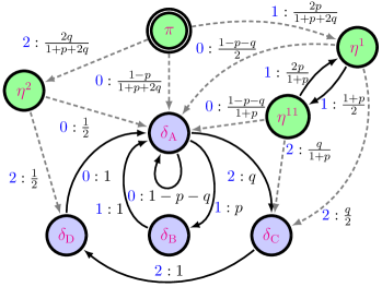
Figure 12: $\mathscr{S}$-MSP of the $(2\text{-}1)$-GP-$(2)$ Process.

As a HMM, the $\epsilon$-machine’s $\mathscr{S}$-MSP is specified by the $4$-tuple: $\mathcal{M}_{\text{{$\mathscr{S}$-MSP}}}=\bigl{(}\bm{\mathcal{R}}_{\pi},\,\mathcal{A},\,\{\mathcal{W}^{({x})}\}_{{x}\in\mathcal{A}},\,\mu_{0}\!=\!\delta_{\pi}\bigr{)}$, where $\bm{\mathcal{R}}_{\pi}$ is the set of mixed states just quoted, $\mathcal{A}$ is the same observable alphabet as before, $\bigl{\{}\mathcal{W}^{({x})}\bigr{\}}_{{x}\in\mathcal{A}}$ is the set of symbol-labeled transition matrices among the mixed states, and $\bra{\delta_{\pi}}=\begin{bmatrix}1&0&0&0&0&0&0&0\end{bmatrix}$ is the start distribution over the mixed states.

With this new linear metadynamic in hand, our next step is to calculate the eigenvalues and projection operators of the internal mixed-state-to-state transition dynamic $\mathcal{W}=\sum_{{x}\in\mathcal{A}}\mathcal{W}^{({x})}$. $\mathcal{W}$ can be explicitly represented in the block-matrix form:

$$\mathcal{W}=\begin{bmatrix}A&B\\ \bm{0}&T\end{bmatrix}~{},$$

where:

$$A =\begin{bmatrix}0&\tfrac{2p}{1+p+2q}&0&\tfrac{2q}{1+p+2q}\\ 0&0&\tfrac{1+p}{2}&0\\ 0&\tfrac{2p}{1+p}&0&0\\ 0&0&0&0\end{bmatrix}~{}\text{and}$$

$$B =\begin{bmatrix}\tfrac{1-p}{1+p+2q}&0&0&0\\ \tfrac{1-p-q}{2}&0&\tfrac{q}{2}&0\\ \tfrac{1-p-q}{1+p}&0&\tfrac{q}{1+p}&0\\ \tfrac{1}{2}&0&0&\tfrac{1}{2}\end{bmatrix}~{},$$

and $T$ is the same as the state-to-state internal transition matrix of the $\epsilon$-machine from earlier.

$\mathcal{W}$’s eigenvalues are thus relatively straightforward to calculate since $\text{det}(\mathcal{W}-\lambda I)=\text{det}(A-\lambda I)\text{det}(T-\lambda I)$ implies that:

$$\Lambda_{\mathcal{W}}=\Lambda_{A}\cup\Lambda_{T}~{}.$$

The new eigenvalues introduced by the feedback matrix $A$ are $\Lambda_{A}=\{0,\pm\sqrt{p}\}$ with $\nu_{0}=2$. While the other eigenvalues ($\pm\sqrt{p}$), found most easily from Part I’s cyclic eigenvalue rule, are associated with diagonalizable subspaces. It is important to note that, while $T$ was only nondiagonalizable along a very special submanifold in parameter space, the mixed-state-to-state metadynamic is generically nondiagonalizable over all parameter settings. This nondiagonalizability corresponds to a special kind of symmetry breaking of uncertainty during synchronization.

$\mathcal{W}$’s eigenvectors are most easily found through a two-step process. Specifically, $\ket{{}^{\pm}\sqrt{p}_{A}}$ and $\bra{{}^{\pm}\sqrt{p}_{A}}$ (the solutions of $A\ket{{}^{\pm}\sqrt{p}_{A}}=\pm\sqrt{p}\ket{{}^{\pm}\sqrt{p}_{A}}$ and $\bra{{}^{\pm}\sqrt{p}_{A}}A=\pm\sqrt{p}\bra{{}^{\pm}\sqrt{p}_{A}}$) are found first, and the result is used to reduce the number of unknowns when solving the full eigenequations ($\mathcal{W}\ket{{}^{\pm}\sqrt{p}_{\mathcal{W}}}=\pm\sqrt{p}\ket{{}^{\pm}\sqrt{p}_{\mathcal{W}}}$) for $\ket{{}^{\pm}\sqrt{p}_{\mathcal{W}}}$ and $\bra{{}^{\pm}\sqrt{p}_{\mathcal{W}}}$. Similarly, we can recycle the restricted eigenvectors $\ket{\lambda_{T}}$ and $\bra{\lambda_{T}}$ found earlier for the $\epsilon$-machine to reduce the number of unknowns when solving the more general eigenvector problems for $\ket{\lambda_{\mathcal{W}}}$ and $\bra{\lambda_{\mathcal{W}}}$ in cases where $\lambda\in\Lambda_{T}$. Performing such a calculation, we find:

$$\ket{{}^{\pm}\sqrt{p}_{\mathcal{W}}} =\begin{bmatrix}\frac{1}{1+p+2q}&\tfrac{\pm\sqrt{p}}{2p}&\tfrac{1}{1+p}&0&0&0&0&0\end{bmatrix}^{\top}~{},$$

$$\bra{{}^{\pm}\sqrt{p}_{\mathcal{W}}} =\begin{bmatrix}0&{}^{\pm}\sqrt{p}&\frac{1+p}{2}&0&-\tfrac{1\pm\sqrt{p}}{2}&-\tfrac{p\pm\sqrt{p}}{2}&0&0\end{bmatrix}~{},$$

$$\bra{\lambda_{\mathcal{W}}} =\begin{bmatrix}0&0&0&0&\lambda^{2}&p\lambda&q\lambda&q\end{bmatrix}\text{ for all }\lambda\in\Lambda_{T}\setminus\{0\}~{},$$

$$\ket{1_{\mathcal{W}}} =\begin{bmatrix}1&1&1&1&1&1&1&1\end{bmatrix}^{\top}~{},\text{ and}$$

$$\ket{\lambda_{\mathcal{W}}} =\begin{bmatrix}0&\frac{\lambda(1+\lambda)}{2}&\frac{\lambda(1+\lambda)}{1+p}&\frac{1+\lambda}{2}&\lambda^{2}&\lambda&1&\lambda\end{bmatrix}^{\top}~{},$$

for $\lambda\in\Lambda_{T}\setminus\{0,1\}$. Moreover, $\mathcal{W}$’s eigenvectors and generalized eigenvector corresponding to eigenvalue $0$ are:

$$\ket{0_{1}^{(1)}} =\bra{\delta_{\pi}}^{\top}=\begin{bmatrix}1&0&0&0&0&0&0&0\end{bmatrix}^{\top}~{},$$

$$\ket{0_{1}^{(2)}} =\begin{bmatrix}0&0&0&\frac{1+p+2q}{2q}&0&0&0&0\end{bmatrix}^{\top}~{},$$

$$\ket{0_{2}^{(1)}} =\begin{bmatrix}0&\frac{1}{2}&\frac{p}{1+p}&\frac{-p}{2q}&0&1&\frac{-p}{q}&0\end{bmatrix}^{\top}~{},$$

$$\bra{0_{1}^{(1)}} =\begin{bmatrix}0&0&0&1&0&0&\frac{-1}{2}&\frac{-1}{2}\end{bmatrix}~{},$$

$$\bra{0_{1}^{(2)}} =\begin{bmatrix}\frac{1+p+2q}{2q}&0&\frac{-(1+p)}{2q}&0&0&0&\frac{-1}{2}&\frac{-1}{2}\end{bmatrix}~{},\text{ and}$$

$$\bra{0_{2}^{(1)}} =\begin{bmatrix}0&0&0&0&0&1&0&-1\end{bmatrix}~{}.$$

Above, we used the notation $\ket{0_{k}^{(m)}}$ for indexing generalized eigenvectors introduced in Part I.

All nondegenerate eigenvalues have projection operators of the form:

$$\mathcal{W}_{\lambda}=\frac{\ket{\lambda}\bra{\lambda}}{\braket{\lambda}{\lambda}}~{}.$$

However, the degenerate and nondiagonalizable subspace associated with the zero eigenvalue has the composite projection operator:

$$\mathcal{W}_{0} =\frac{\ket{0_{1}^{(1)}}\bra{0_{1}^{(2)}}}{\braket{0_{1}^{(2)}}{0_{1}^{(1)}}}+\frac{\ket{0_{1}^{(2)}}\bra{0_{1}^{(1)}}}{\braket{0_{1}^{(1)}}{0_{1}^{(2)}}}+\frac{\ket{0_{2}^{(1)}}\bra{0_{2}^{(1)}}}{\braket{0_{2}^{(1)}}{0_{2}^{(1)}}}~{}.$$

The fact that $\bra{\delta_{\pi}}\lambda_{\mathcal{W}}\rangle=0$ for all $\lambda\in\Lambda_{T}\setminus\bigl{(}\{1\}\cup\Lambda_{A}\bigr{)}$ is an instantiation of a general result that greatly simplifies the calculations relating to predictability and prediction.

The remaining piece for analyzing predictability is the vector of transition-entropies $\ket{\operatorname{H}(W^{\mathcal{A}})}$. A simple calculation, utilizing the fact that:

$$-\sum_{i}\frac{n_{i}}{d}\log\left(\frac{n_{i}}{d}\right)=\log(d)-\frac{1}{d}\sum_{i}n_{i}\log n_{i}~{},$$

when $\sum_{i}n_{i}=d$, yields:

$$\ket{\operatorname{H}(W^{\mathcal{A}})}=\begin{bmatrix}\log(1+p+2q)-\frac{1}{1+p+2q}\bigl{[}2q\log(2q)+2p\log(2p)+(1-p)\log(1-p)\bigr{]}\\ 1-\frac{1}{2}\bigl{[}q\log(q)+(1+p)\log(1+p)+(1-p-q)\log(1-p-q)\bigr{]}\\ \log(1+p)-\frac{1}{1+p}\bigl{[}q\log(q)+2p\log(2p)+(1-p-q)\log(1-p-q)\bigr{]}\\ 1\\ -\bigl{[}q\log(q)+p\log(p)+(1-p-q)\log(1-p-q)\bigr{]}\\ 0\\ 0\\ 0\end{bmatrix}~{},$$

where $\log$ is understood to be the base-2 logarithm $\log_{2}$.

Putting this all together, we can now calculate in full detail the myopic entropy rate $h_{\mu}(L)$ that results from modeling the infinite-order $(2\text{-}1)$-GP-$(2)$ process as an order-$(L\text{-}1)$ Markov process:

$$h_{\mu}(L) =\sum_{\lambda\in\Lambda_{W}\atop\lambda\neq 0}\sum_{m=0}^{\nu_{\lambda}-1}\bra{\delta_{\pi}}W_{\lambda,m}\ket{\operatorname{H}(W^{\mathcal{A}})}\binom{L-1}{m}\lambda^{L-1-m}$$

$$\quad+\left[0\in\Lambda_{W}\right]\sum_{m=0}^{\nu_{0}-1}\delta_{L-1,m}\bra{\delta_{\pi}}W_{0}W^{m}\ket{\operatorname{H}(W^{\mathcal{A}})}$$

$$=\delta_{L,1}\bra{\delta_{\pi}}W_{0}\ket{\operatorname{H}(W^{\mathcal{A}})}+\delta_{L,2}\bra{\delta_{\pi}}WW_{0}\ket{\operatorname{H}(W^{\mathcal{A}})}$$

$$\quad+\bra{\delta_{\pi}}W_{1}\ket{\operatorname{H}(W^{\mathcal{A}})}+\!\!\!\!\!\sum_{\lambda\in\Lambda_{W}\setminus\Lambda_{T}}\!\!\!\!\!\bra{\delta_{\pi}}W_{\lambda}\ket{\operatorname{H}(W^{\mathcal{A}})}\lambda^{L-1}.$$

This oscillates under an exponentially decaying envelope as it approaches its asymptotic value of:

$$h_{\mu} =\bra{\delta_{\pi}}W_{1}\ket{\operatorname{H}(W^{\mathcal{A}})}$$

$$=\bra{\delta_{\pi}}1_{\mathcal{W}}\rangle\langle\pi_{\mathcal{W}}\ket{\operatorname{H}(W^{\mathcal{A}})}$$

$$=\langle\pi_{\mathcal{W}}\ket{\operatorname{H}(W^{\mathcal{A}})}=\braket{\pi_{T}}{\operatorname{H}(T^{\mathcal{A}})}$$

$$=\frac{-q\log q-p\log p-(1-p-q)\log(1-p-q)}{1+p+2q}~{}.$$

Simplifying the terms in the myopic entropy rate yields:

$$\bra{\delta_{\pi}}W_{0}\ket{\operatorname{H}(W^{\mathcal{A}})} =\langle\delta_{\pi}\ket{\operatorname{H}(W^{\mathcal{A}})}$$

$$\qquad-\frac{1+p}{1+p+2q}\langle\delta_{\eta^{11}}\ket{\operatorname{H}(W^{\mathcal{A}})}$$

and:

$$\bra{\delta_{\pi}}WW_{0}\ket{\operatorname{H}(W^{\mathcal{A}})}=\frac{2q}{1+p+2q}$$

for the two ephemeral contributions.

For $L\geq 3$, we find for odd $L$:

$$h_{\mu}(L)-h_{\mu} =\frac{-p\log p+(1+p)\log(1+p)-2p}{\sqrt{p}(1+p+2q)}\,p^{L/2}$$

and for even $L$:

$$h_{\mu}(L)-h_{\mu} =\frac{p\log p-(1+p)\log(1+p)+2}{1+p+2q}\,p^{L/2}~{}.$$

This highlights the period-2 nature of the asymptotic decay.

The total mutual information between the observable past and observable future, the excess entropy, is:

$${\bf E} =\!\!\!\sum_{\lambda\in\Lambda_{W}\setminus\{1\}}\sum_{m=0}^{\nu_{\lambda}-1}\frac{1}{(1-\lambda)^{m+1}}\bra{\delta_{\pi}}W_{\lambda,m}\ket{\operatorname{H}(W^{\mathcal{A}})}$$

$$=\frac{(1-p-q)\log(1-p-q)-p\log p}{1+p+2q}$$

$$\qquad-\frac{q\log q+(1-p)\log(1-p)}{1+p+2q}$$

$$\qquad+\log(1+p+2q)~{}.$$

This is the total future information that can possibly be predicted using past observations. The structure of how this information is unraveled over time is revealed in the excess entropy spectrum:

$$\mathcal{E}(\omega) =\pi h_{\mu}\delta(\omega)$$

$$\qquad+\sum_{m=0}^{\nu_{0}-1}\cos\bigl{(}(m+1)\,\omega\bigr{)}\bra{\delta_{\pi}}W_{0}W^{m}\ket{\operatorname{H}(W^{\mathcal{A}})}$$

$$\qquad+\sum_{\lambda\in\Lambda_{W}\setminus 0}\sum_{m=0}^{\nu_{\lambda}-1}\text{Re}\biggl{(}\frac{\bra{\delta_{\pi}}W_{\lambda,m}\ket{\operatorname{H}(W^{\mathcal{A}})}}{(e^{i\omega}-\lambda)^{m+1}}\biggr{)}$$

$$=\pi h_{\mu}\delta(\omega)+\frac{2q}{1+p+2q}\cos(2\omega)$$

$$\qquad+\bigl{(}{\bf E}+\frac{p\log p-(1+p)\log(1+p)-2q}{1+p+2q}\bigr{)}\cos(\omega)$$

$$\qquad+\frac{-p\log p+(1+p)\log(1+p)}{1+p+2q}\text{Re}\biggl{(}\frac{e^{i\omega}-p}{e^{i2\omega}-p}\biggr{)}$$

$$\qquad+\tfrac{2p}{1+p+2q}\text{Re}\biggl{(}\frac{1-e^{i\omega}}{e^{i2\omega}-p}\biggr{)}~{}.$$

From this, we observe that ${\bf E}=\lim_{\omega\to 0}\mathcal{E}(\omega)$.

A.4 Synchronizing to predict optimally

To analyze the information-processing cost of synchronizing to a process, we need its $\epsilon$-machine $\mathscr{S}$-MSP. We already constructed this in the last section. Hence, we can immediately evaluate the resources necessary for synchronizing to and predicting the $(2\text{-}1)$-GP-$(2)$ Process.

The only novel piece needed for this is the vector of mixed-state entropies $\ket{\operatorname{H}[\eta]}$. A simple calculation yields:

$$\ket{\operatorname{H}[\eta]}=\begin{bmatrix}\log(1+p+2q)-\tfrac{p\log p+2q\log q}{1+p+2q}\\ 1\\ \log(1+p)-\tfrac{p\log p}{1+p}\\ 1\\ 0\\ 0\\ 0\\ 0\end{bmatrix}~{},$$

where $\log$ is again understood to be the base-2 logarithm $\log_{2}$.

An observer, tasked with predicting the future as well as possible, must synchronize to the causal state of the dynamic. During the metadynamics of synchronization, the observer on average will pick up synchronization information according to the remaining causal-state uncertainty $\mathcal{H}^{+}(L)$ after an observation interval of $L$ steps:

$$\mathcal{H}^{+}(L)$$

$$=\sum_{\lambda\in\Lambda_{\mathcal{W}}\atop\lambda\neq 0}\sum_{m=0}^{\nu_{\lambda}-1}\bra{\delta_{\pi}}\mathcal{W}_{\lambda,m}\ket{\operatorname{H}[\eta]}\binom{L}{m}\lambda^{L-m}$$

$$\qquad+\left[0\in\Lambda_{\mathcal{W}}\right]\sum_{m=0}^{\nu_{0}-1}\delta_{L,m}\bra{\delta_{\pi}}\mathcal{W}_{0}\mathcal{W}^{m}\ket{\operatorname{H}[\eta]}$$

$$=\delta_{L,0}\bigl{[}\log(1+p+2q)-\frac{2q\log q+(1+p)\log(1+p)}{1+p+2q}\bigr{]}$$

$$\qquad+\delta_{L,1}\tfrac{2q}{1+p+2q}+\frac{\langle\sqrt{p}\ket{\operatorname{H}[\eta]}+(-1)^{L}\langle^{-}\!\sqrt{p}\ket{\operatorname{H}[\eta]}}{1+p+2q}\,p^{L/2}~{}.$$

More explicitly, for $L\geq 2$, this becomes:

$$\mathcal{H}^{+}(L) =\begin{cases}\frac{2\sqrt{p}}{1+p+2q}\,p^{L/2}&\text{ \small for odd }L\\ \frac{(1+p)\log(1+p)-p\log p}{1+p+2q}\,p^{L/2}&\text{ \small for even }L\end{cases}~{}.$$

The total synchronization information accumulated is then:

$${\bf S} =\!\!\!\sum_{\lambda\in\Lambda_{\mathcal{W}}\setminus\{1\}}\sum_{m=0}^{\nu_{\lambda}-1}\frac{1}{(1-\lambda)^{m+1}}\bra{\delta_{\pi}}\mathcal{W}_{\lambda,m}\ket{\operatorname{H}[\eta]}$$

$$=\frac{2q(1-\log q)}{1+p+2q}+\frac{p\bigl{[}2-\log p+(1+p)\log(1+p)\bigr{]}}{(1-p)(1+p+2q)}$$

$$\qquad+\log(1+p+2q)~{}.$$

Even after synchronization, an observer must update an average of $b_{\mu}$ of its bits of information per observation and must keep track of a net $C_{\mu}$ bits of information to stay synchronized, where:

$$C_{\mu} =\operatorname{H}[\pi]$$

$$=\langle\delta_{\pi}\ket{\operatorname{H}[\eta]}$$

$$=\log(1+p+2q)-\frac{p\log p+2q\log q}{1+p+2q}~{}.$$

An interesting feature of prediction is a process’ crypticity:

$$\chi =C_{\mu}-{\bf E}$$

$$=\frac{3q\log q+(1-p)\log(1-p)}{1+p+2q}$$

$$\qquad-\frac{(1-p-q)\log(1-p-q)}{1+p+2q}~{},$$

This gives, as a function of $p$ and $q$, the minimal overhead of additional memory about the past—beyond the information that the future can possibly share with it—that must be stored for optimal prediction.

In summary, we now more fully appreciate, via this rather complete analysis, the fundamental limits on predictability of our example stochastic process. It showed many of the qualitative features, both in terms of the calculation and system behavior, that should be expected when analyzing prediction, based on the more general results of the main development. The procedures can be commandeered to apply to any inference algorithm that yields a generative model, whether classical machine learning, Bayesian Structural Inference [10], or any other favorite inference tool. With a generative model in hand, synchronizing to real world data—necessary to make good predictions about the real world’s future—follows the $\mathscr{S}$-MSP metadynamics. The consequences for prediction is that typically there will be a finite epoch of symmetry collapse followed by a slower asymptotic synchronization that allows improved prediction, as longer observations induce a refined knowledge of what lies hidden.

References

- [1] S. E. Marzen and J. P. Crutchfield. Nearly maximally predictive features and their dimensions. Phys. Rev. E, 95(5):051301(R), 2017.
- [2] P. M. Riechers and J. P. Crutchfield. Beyond the spectral theorem: Decomposing arbitrary functions of nondiagonalizable operators. arxiv.org:1607.06526.
- [3] T. M. Cover and M. E. Hellman. The two-armed-bandit problem with time-invariant finite memory. IEEE Trans. Info. Th., 16(2):185–195, Mar 1970.
- [4] J. P. Crutchfield and S. E. Marzen. Signatures of infinity: Nonergodicity and resource scaling in prediction, complexity, and learning. Phys. Rev. E, 91:050106(R), 2015.
- [5] J. P. Crutchfield and D. P. Feldman. Regularities unseen, randomness observed: Levels of entropy convergence. CHAOS, 13(1):25–54, 2003.
- [6] P. M. Riechers, D. P. Varn, and J. P. Crutchfield. Diffraction patterns of layered close-packed structures from hidden markov models. arxiv.org:1410.5028.
- [7] D. Lind and B. Marcus. An Introduction to Symbolic Dynamics and Coding. Cambridge University Press, New York, 1995.
- [8] B. Latni. Signal processing and linear systems. Oxford University Press, USA, 1998.
- [9] Historically, the name “Golden Mean” derives from the -Golden Mean Process that forbids two consecutive s. It describes the symbolic dynamics of the chaotic one-dimensional shift map over the unit interval with generating partition, when the slope of the map is the golden mean [11]. Moreover, consistency with the stationary stochastic process generated implies . Generalizing to arbitrary and especially to arbitrary and takes us away from the eponymous property into a setting sufficiently general to study the generic behavior of order- Markov processes and the complexities of predicting them.
- [10] C. C. Strelioff and J. P. Crutchfield. Bayesian structural inference for hidden processes. Phys. Rev. E, 89:042119, Apr 2014.
- [11] S. G. Williams. Introduction to symbolic dynamics. In Proceedings of Symposia in Applied Mathematics, volume 60, pages 1–12, 2004.