Multiple Kernel Learning and Automatic Subspace Relevance Determination for High-dimensional Neuroimaging Data

Abstract

Alzheimer’s disease is a major cause of dementia. Its diagnosis requires accurate biomarkers that are sensitive to disease stages. In this respect, we regard probabilistic classification as a method of designing a probabilistic biomarker for disease staging. Probabilistic biomarkers naturally support the interpretation of decisions and evaluation of uncertainty associated with them. In this paper, we obtain probabilistic biomarkers via Gaussian Processes. Gaussian Processes enable probabilistic kernel machines that offer flexible means to accomplish Multiple Kernel Learning. Exploiting this flexibility, we propose a new variation of Automatic Relevance Determination and tackle the challenges of high dimensionality through multiple kernels. Our research results demonstrate that the Gaussian Process models are competitive with or better than the well-known Support Vector Machine in terms of classification performance even in the cases of single kernel learning. Extending the basic scheme towards the Multiple Kernel Learning, we improve the efficacy of the Gaussian Process models and their interpretability in terms of the known anatomical correlates of the disease. For instance, the disease pathology starts in and around the hippocampus and entorhinal cortex. Through the use of Gaussian Processes and Multiple Kernel Learning, we have automatically and efficiently determined those portions of neuroimaging data. In addition to their interpretability, our Gaussian Process models are competitive with recent deep learning solutions under similar settings.

Keywords— Statistical learning; Classification algorithms; Bayesian methods; Gaussian processes; Magnetic Reasonance Imaging; Alzheimer’s Disease;

1 Introduction

Alzheimer’s disease (AD) is the 6^th leading cause of death in the United States [1]. Its pathology induces complex patterns that evolve as the disease progresses [22]. The pathology mainly starts in and around the hippocampus and entorhinal cortex; however, by the time of a clinical diagnosis, the cerebral atrophy is widespread and it involves, to a large extent, temporal, parietal, and frontal lobes [72, 22]. Moreover, the AD pathology does not necessarily conform to anatomical boundaries [22]. Thus, it is highly recommended that the entire brain, instead of predetermined regions of interest (ROI), be examined for accurate diagnosis [72, 22].

The most recent criteria and guidelines for AD diagnosis, as proposed by the National Institute on Aging (NIA) and the Alzheimer’s Association (AA), describe a continuum in which an individual experiences a smooth transition from functioning normally, despite the changes in the brain, to failing to compensate for the deterioration of cognitive abilities [1]. There are three stages of AD: i) preclinical AD, ii) Mild Cognitive Impairment (MCI)due to AD, and iii) dementia due to AD. In the preclinical stage, measurable physiological changes may be observed; however, the symptoms are not developed [1]. MCI is a transitional state between normal aging and AD [55]. Individuals with MCI experience measurable changes in their cognitive abilities, which are also notable by family and friends, but the symptoms are not significant enough to affect the patient’s daily life [1]. On the downside, MCI shares features with AD and it is likely to progress to AD at an accelerated rate [55].

1.1 Biomarkers

A biomarker quantifies a biological state, i.e., the presence or absence of a disease, or the risk of developing a particular condition. According to the World Health Organization (WHO), “any substance, structure or process that can be measured in the body or its products and influence or predict the incidence of outcome or disease” is a biomarker [73]. Examples include blood glucose level for diabetes, cholesterol level for heart disease risk, and body mass index (BMI) for obesity. Ideally, a biomarker is safe, easy to measure, repeatable, and sensitive and specific to the state or condition targeted.

The guidelines for AD diagnosis identify biomarkers that measure i) the amyloid-beta (A$\beta$) accumulation in the brain and ii) if the neurons in the brain are injured or degenerating [1]. These biomarkers will be essential to identify the disease during the preclinical or MCI stages, administer disease-modifying treatments, and monitor the progression towards AD. However, more research is needed to evaluate the effectiveness of these biomarkers and investigate potential combinations of them for more accurate screening [1].

Neuroimaging techniques such as Positron Emission Tomography (PET) and Magnetic Resonance Imaging (MRI) are useful in identifying brain changes due to tumors and other damages that can explain a patient’s symptoms. As a result, they have been used as imaging biomarkers [47]. However, it is virtually impossible to visually detect a slight decrease in regional cerebral blood flow or glucose metabolism in cases of early AD [37]. Also, such an inspection is susceptible to other factors like subjectivity and experience of the physician [47, 38]. On the other hand, voxel-based representations of neuroimagery can be used to perform both standardization and data-driven analysis of brain imagery [51, 47].

1.2 Computerized Diagnosis

Klöppel et al. [38] compared the accuracy of dementia diagnosis provided by radiologists to that of a computer-based diagnostic method. Basically, they extracted the segments of gray matter (GM) from complete MRI scans, normalized them into a standard template, and ended up with several thousands of voxels. Then, they used Support Vector Machines (SVMs) for binary classification problems: i) healthy (normal) vs. AD and ii) fronto-temporal lobar degeneration vs. AD. They also recruited radiologists with different levels of experience for the same problems. The well-trained and experienced radiologists are competitive with the computerized method; however, the overall performance of radiologists is susceptible to human factors [38]. As a result, the radiologists induce a larger variance in the diagnostic accuracy. In this regard, Klöppel et al. [38] argue that the accuracy of the computerized diagnosis of AD is equal to or better than that of radiologists.

In summary, a general adoption of computerized methods for visual image interpretation for dementia diagnosis is strongly recommended [51, 37, 47, 38]. Given the variety of computational methods and growing interest of researchers from a diverse set of disciplines, better diagnostic tools are also expected in the near future. In this respect, Klöppel et al. [38] stress the need for further research on probabilistic methods because medical experts could have more comfort from knowing the confidence levels associated with decisions and having better ability to interpret the models behind them.

1.3 Motivation of Work

Machine learning algorithms can be viewed in two main categories: discriminative and generative. Discriminative algorithms exploit labeled training data in order to uncover input–output relations. These methods can demonstrate excellent generalization performances even though little is known about the generating mechanisms of data. On the other hand, generative methods aim to capture the generating mechanisms of data and to discover the structure of classes [70]. However, unless the representation extracted by a generative method completely epitomizes reality, its generalization performance is usually poor.

The cost of neuroimaging data is high since the gathering process involves expensive imaging procedures and domain experts. Thus, sample sizes are small. Also, neuroimaging procedures usually generate high-dimensional data. An attempt to examine the complete brain imagery complicates statistical analysis and modeling, resulting in high computational complexity, and typically more sophisticated and perhaps less comprehensible models.

Due to the complexity of atrophy patterns and high dimensionality of data, we have resorted to discriminative methods and focused on a particular family of algorithms known as kernel machines. SVM is probably the best known kernel machine and it has been the workhorse of the multivariate predictive analysis of brain data [38, 22, 31, 4, 82, 79, 32, 6]. The popularity of SVM is mainly due to its theoretical soundness and guarantees on generalization performance in spite of high dimensionality. However, SVM characteristically lacks the support for probabilistic interpretation of the decision function and evaluation of uncertainty associated with decisions. Even though solutions (Section 2.1.1) have been proposed to calibrate the SVM outputs for probabilistic information, these procedures are ad hoc instead of being an integral part of the SVM framework. On the other hand, Gaussian Processes (GPs) enable a holistic view of Bayesian probability theory that meets with the need for computational tractability [59]. The result is a probabilistic kernel machine with comprehensive support for interpretability. For instance, a GP model can execute a process known as Automatic Relevance Determination (ARD) [46, 52] by means of specialized kernel functions. The process yields an explanatory and sparse subset of features [76]. But, the high dimensionality of neuroimaging data has rendered ARD too expensive for this context.

In this study, we regard the induction of a classifier as the creation of a computational biomarker for disease staging. Analogously, the creation of a probabilistic classifier results in a probabilistic (computational) biomarker. We propose to design probabilistic biomarkers via GPs. Also, GPs offer flexible means to carry out the Multiple Kernel Learning (MKL) and tackle the challenges of high dimensionality. In this regard, we first investigate the conventional single kernel learning and postulate the advantages of using GP models rather than SVMs for biomarker induction. Then, we extend the basic scheme towards MKL and propose a new variation of ARD, namely, the Multiple Kernel Learning for Automatic Subspace Relevance Determination (MKL-AsRD). It inherits the supervised feature selection characteristics of ARD and unites them with the automatic model selection capabilities of MKL. In contrast to sparse variants of GPs, such as the Relevance Vector Machine (RVM) and Sparse Pseudo-Input Gaussian Process (SPGP), MKL-AsRD takes advantage of the full (non-sparse) GPs. Despite the use of full GPs, MKL-AsRD is computationally feasible for the high-dimensional neuroimaging data. It has improved the performance of probabilistic biomarkers. Moreover, the proposed models are competitive with deep learning solutions under similar settings.

The rest of the document is organized as follows. Section 2 reviews kernel machines and the basics of MKL. Section 3 introduces MKL-AsRD. Section 4 presents the experiments and results. Section 5 compares and contrasts our work with previous methods including the deep learning solutions. Section 6 concludes the study.

2 Kernel Machines

Kernel machines translate the data points into an Euclidean feature space and aim to solve the machine learning problems in the new space. In this review section, we focus on supervised learning problems, for which the goal is to learn an appropriate function $y=f(\mathbf{x})$, where $\mathbf{x}=(x_{1},x_{2},...,x_{D})$ and $D$ is the number of dimensions, that maps inputs to outputs, given a data set $\mathcal{D}=\{(\mathbf{x}_{i},y_{i})\}$ where $i=1...N$.

In the context of kernel machines, it is assumed that there is a function $\phi(\mathbf{x})$ that translates inputs into a feature space and a kernel function $k(\mathbf{x}_{i},\mathbf{x}_{j})=\phi(\mathbf{x}_{i})\phi(\mathbf{x}_{j})^{T}$ implicitly achieves an embedding of observations into the feature space and yields the inner products. As a result, there is no need to explicitly compute the feature vectors and corresponding inner products. This is known as the kernel trick [62, 59]. A kernel that induces positive semidefinite (PSD) Gram matrices is said to be PSD. A PSD kernel guarantees the uniqueness of a Reproducing Kernel Hilbert Space (RKHS) [62, 59]. The existence of RKHS allows us to use various distance measures that are accepted by Mercer’s theorem [49].

In the next subsection, we review the well-known SVM and point out its disadvantages regarding model selection and probabilistic outputs. Then, we discuss the fundamentals of GPs and emphasize their capabilities for factor analysis and dimensionality reduction. We also review the special cases of GP models such as RVM and SPGP as they address the relevance determination and sparsity in different ways.

2.1 Support Vector Machine

A typical SVM formulation for classification is

$$\min_{w,b,\varepsilon} \frac{1}{2}\mathbf{w}^{T}\mathbf{w}+C\sum_{i=1}^{N}\varepsilon_{i}$$ (1)

$$s.t. y_{i}(\mathbf{w}^{T}\mathbf{x}_{i}+b)\geq 1-\varepsilon_{i}$$

$$\varepsilon_{i}\geq 0,\quad i\in\{1,\dots,N\},$$

where $C>0$ is the regularization parameter [71, 14]. This formulation is also known as $C$-Support Vector Classification ($C$-SVC). The dual of (1) is written as

$$\min_{w,b,\varepsilon} \frac{1}{2}{\boldsymbol{\alpha}}^{T}Q{\boldsymbol{\alpha}}-\mathbf{e}^{T}{\boldsymbol{\alpha}}$$ (2)

$$s.t. \mathbf{y}^{T}{\boldsymbol{\alpha}}=0,$$

$$0\leq\alpha_{i}\leq C,\quad i\in\{1,\dots,N\},$$

where $\mathbf{e}=[1,\dots,1]^{T}$, $Q$ is an $N\times N$ PSD matrix, $Q_{ij}=y_{i}y_{j}k(\mathbf{x}_{i},\mathbf{x}_{j})$ and $k(\mathbf{x}_{i},\mathbf{x}_{j})$ is a kernel function [14]. A typical choice is a Radial Basis Function (RBF) (3):

$$k_{RBF}(\mathbf{x}_{i},\mathbf{x}_{j})=\text{exp}\left(-\gamma{\parallel}\mathbf{x}_{i}-\mathbf{x}_{j}{\parallel}^{2}\right).$$ (3)

Once (2) is solved for $\boldsymbol{\alpha}$, the SVM decision function is

$$f(\mathbf{x}_{*})=\text{sgn}\left(\sum_{i=1}^{N}y_{i}\alpha_{i}k(\mathbf{x}_{i},\mathbf{x}_{*})+b\right),$$ (4)

where $b$ is the intercept term. For $\alpha_{i}\neq 0$, $\mathbf{x}_{i}$ is a support vector. An SVM solution is sparse in the sense that the decision function depends only on support vectors. Also note that the output is a class label ($-1\text{ or }+1$) [14].

Training a typical SVM with an RBF kernel involves an exhaustive grid search for the values of hyperparameters $C$ and $\gamma$ [14] . For a large number of parameter configurations, the grid search becomes prohibitively expensive. In practice, the search is conducted with respect to a finite set of discrete parameter configurations predefined by user. Namely, the user roughly predicts the search space in which likely solutions exist. Then, for each configuration, (2) must be solved for $\boldsymbol{\alpha}$ in order to obtain (4). Moreover, each decision function must be evaluated on a validation set in the search of the most plausible model. The validation set is essentially a portion of the valuable training data. Consequently, the solution to (2) is derived from a smaller training set. In this regard, Chang and Lin [14] suggest that the validation set be added to the training set, once the kernel parameters are optimized, and (2) be solved again in order to obtain the final model. However, such retraining does not necessarily mean that it will improve the model because SVM is a stable algorithm robust to perturbation of examples under mild conditions [62, 78].

2.1.1 Probabilistic Outputs

The SVM outputs can be calibrated so as to generate probabilistic information [56]. A sigmoid function, $\lambda(af(\mathbf{x})+b)$, is fitted to the training set. Based on the solution of Platt [56], Lin et al. [44] introduced a more robust algorithm with decent convergence properties. Using class labels and decision values, $a$ and $b$ are estimated by maximizing the likelihood of training data [77, 14]. Since such a training may cause the model to overfit to the data, a second-level cross-validation (CV) is required in order to obtain acceptable decision values [77, 14]. Unfortunately, it causes a major overhead regarding the model selection due to nested validation procedures.

2.2 Gaussian Processes for Regression

GPs enable us to do inference in the function space. Explicitly, given $\mathcal{D}$, an $N$-dimensional random vector $\mathbf{f}$ represents the function values induced by inputs. We wish to infer the best possible $\mathbf{f}$ in order to match to the target vector $\mathbf{y}$.

A GP is specified by a mean function $m(\mathbf{x}_{i})$ and a covariance function $k(\mathbf{x}_{i},\mathbf{x}_{j})$. Given an observation $\mathbf{x}_{i}$ as input, the value of $f(\mathbf{x}_{i})$ is a sample from the process [59]:

$$f(\mathbf{x}_{i}) \sim\mathcal{GP}(m(\mathbf{x}_{i}),k(\mathbf{x}_{i},\mathbf{x}_{j}))\text{, where}$$ (5)

$$m(\mathbf{x}_{i}) =\mathbb{E}[f(\mathbf{x}_{i})]$$

$$k(\mathbf{x}_{i},\mathbf{x}_{j}) =\mathbb{E}[(f(\mathbf{x}_{i})-m(\mathbf{x}_{i}))(f(\mathbf{x}_{j})-m(\mathbf{x}_{j}))]\text{.}$$

(5) indicates that $f(\mathbf{x}_{i})$ and $f(\mathbf{x}_{j})$ are jointly Gaussian. For $j=1...N$, $f(\mathbf{x}_{i})$ depends on other observations, as well. In this regard, a GP model that uses all observations is considered to be full (non-sparse) and special cases of GP models that provide sparse approximations (Section 2.5 and Section 2.6) to full GPs exist [69, 12, 59, 63, 64].

In GP learning, inner products are computed with respect to a covariance matrix $\Sigma_{f}$ implied by the features: $k(\mathbf{x}_{i},\mathbf{x}_{j})=\phi(\mathbf{x}_{i})\Sigma_{f}\phi(\mathbf{x}_{j})^{T}$ [59]. Hence, in GP terminology, a kernel is a covariance function that estimates the covariance of two latent variables $f(\mathbf{x}_{i})$ and $f(\mathbf{x}_{j})$ in terms of input vectors $\mathbf{x}_{i}$ and $\mathbf{x}_{j}$ [59]. A simple covariance function that depends on an inner product of the input vectors is $k_{LIN}(\mathbf{x}_{i},\mathbf{x}_{j})={\sigma^{2}_{f}}\left(\mathbf{x}_{i}{\cdot}\mathbf{x}_{j}^{T}\right)$, where $\sigma_{f}$ is the scale parameter. A more widely used one is the squared-exponential (SE) covariance function:

$$k_{SE}(\mathbf{x}_{i},\mathbf{x}_{j})={\sigma^{2}_{f}}\text{exp}\left(-\frac{{\parallel}\mathbf{x}_{i}-\mathbf{x}_{j}{\parallel}^{2}}{2{\ell}^{2}}\right),$$ (6)

where $\ell$ is the bandwidth parameter. Another example is the neural network (NN) covariance function:

$$k_{NN}(\mathbf{x}_{i},\mathbf{x}_{j})={\sigma^{2}_{f}}\text{sin}^{-1}\left(\frac{2\mathbf{\tilde{x}}_{i}^{T}\Sigma\mathbf{\tilde{x}}_{j}}{\sqrt{(1+2\mathbf{\tilde{x}}_{i}^{T}\Sigma\mathbf{\tilde{x}}_{i})(1+2\mathbf{\tilde{x}}_{j}^{T}\Sigma\mathbf{\tilde{x}}_{j})}}\right),$$ (7)

where $\tilde{\mathbf{x}}=(1,\mathbf{x})^{T}$ is an augmented input vector and $\Sigma$ is a covariance matrix for input-to-hidden weights: $\mathbf{w}\sim\mathcal{N}(\mathbf{0},\Sigma)$ [52, 75, 59]. A GP with the NN covariance function emulates a NN with a single hidden layer [59].

2.2.1 Learning of hyperparameters

A GP-prior, e.g., $\mathbf{f}\sim\mathcal{N}(\mathbf{0},K)$, is a prior distribution over the latent variables. The covariance matrix $K$ is dictated by the covariance function $k(\cdot,\cdot)$. Once combined with the likelihood associated with observed data, the GP-prior leads to a GP-posterior in a function space. This Bayesian treatment promotes the smoothness of predictive functions [75] and the prior has an effect analogous to the quadratic penalty term used in maximum-likelihood procedures [59].

The impact of the covariance function on the information processing capabilities of GPs is larger for small to medium-sized datasets [21]. As the covariance function communicates our beliefs about the functions to be estimated, it should suit the problem at hand well. Otherwise, the likelihood term may fail to compensate for the inappropriate prior specification unless the dataset is large enough.

Many covariance functions have adjustable parameters, such as $\ell$ and $\sigma_{f}$ in (6). In this regard, learning in GPs is equivalent to finding suitable parameters for the covariance function. Given the target vector $\mathbf{y}$ and the matrix $X$ that consists of training instances, this is accomplished by maximizing the log marginal likelihood function:

$$\text{log }p(\mathbf{y}|X)=\underbrace{-\frac{1}{2}\mathbf{y}^{T}(K+\sigma^{2}_{n}I)^{-1}\mathbf{y}}_{\text{data fit term}}\underbrace{-\frac{1}{2}\text{log }|K+\sigma^{2}_{n}I|}_{\text{complexity term}}\underbrace{-\frac{N}{2}\text{log }2{\pi}}_{\text{a constant}},$$ (8)

where $\sigma_{n}$ is due to the Gaussian noise model, $y_{i}=f_{i}+\varepsilon$ and $\varepsilon\sim\mathcal{N}(0,\sigma^{2}_{n})$. Note that a large number of hyperparameters can be automatically approximated by maximizing (8) via continuous optimization. (8) is solved just once and no validation set is required, which is desirable when the sample size is small.

2.2.2 Predictions

GP regression yields a predictive Gaussian distribution (9), from which a prediction $f_{*}=f(\mathbf{x}_{*})$ is sampled, given the training instances $X$, target vector $\mathbf{y}$ and test input $\mathbf{x}_{*}$.

$$f_{*}|X,\mathbf{y},\mathbf{x}_{*}\sim\mathcal{N}(\bar{f}_{*},\mathbb{V}[f_{*}])\text{, where}$$ (9)

$$\bar{f}_{*}=\mathbf{k}_{*}^{T}(K+\sigma^{2}_{n}I)^{-1}\mathbf{y}$$ (10)

$$\mathbb{V}[f_{*}]=k(\mathbf{x}_{*},\mathbf{x}_{*})-\mathbf{k}_{*}^{T}(K+\sigma^{2}_{n}I)^{-1}\mathbf{y}$$ (11)

and $\mathbf{k}_{*}$ is a vector of covariances between the test input $\mathbf{x}_{*}$ and the training instances. (10) gives the mean prediction $\bar{f}_{*}$, which is the empirical risk minimizer for any symmetric loss function [59]. (11) yields the predictive variance. Notice that the information extracted from the observations reduces the prior variance.

2.3 Gaussian Processes for Classification

Logistic regression (LR) is a well-known binary classifier, for which a sigmoid function (12) assigns the class probabilities of a given input $\mathbf{x}_{*}$ based on the associated function value $f_{*}$:

$$p(y_{*}=+1|\mathbf{x}_{*})=\lambda(f_{*})=\frac{1}{1+\text{exp}(-f_{*})}.$$ (12)

GP classification generalizes the idea and turns $\lambda(f_{*})$ into a stochastic function, which implies a distribution over predictive probabilities. Once the nuisance parameters are integrated out, we obtain the averaged predictive probability via (13) and (14) [59].

$$\bar{\lambda}(f_{*})=\int\lambda(f_{*})p(f_{*}|X,\mathbf{y},\mathbf{x}_{*})df_{*},\text{ where}$$ (13)

$$p(f_{*}|X,\mathbf{y},\mathbf{x}_{*})=\int p(f_{*}|X,\mathbf{x}_{*},\mathbf{f})p(\mathbf{f}|X,\mathbf{y})d\mathbf{f}$$ (14)

Due to discrete targets, the likelihood term is not Gaussian. Neither is the posterior distribution over the functions, $p(\mathbf{f}|X,\mathbf{y})$. Thus, the exact computation in (14) is intractable and we resort to approximation methods. A comprehensive overview of algorithms for approximate inference in GPs for probabilistic binary classification is provided [53]. We consider two of these solutions: Laplace Approximation (LA) and Expectation Propagation (EP).

2.3.1 Laplace Approximation

LA proposes a second order Taylor expansion around the mode of the posterior distribution and replaces $p(\mathbf{f}|X,\mathbf{y})$ with a Gaussian approximation $q(\mathbf{f}|X,\mathbf{y})$ centered at the Maximum-a-Posteriori (MAP) estimate of $p(\mathbf{f}|X,\mathbf{y})$. The covariance matrix of the approximation is given by the inverse of the Hessian of negative log-posterior [75, 59, 53].

LA is a local method that exploits the properties, such as derivatives, of the posterior at a particular location only, e.g., at the posterior distribution’s mode [53]. Owing to its simplicity, LA is very fast; however, this method may lead to substantial underestimations of the mean and covariance, especially, in high-dimensional spaces because the mode and mean can be far from each other [40, 53].

2.3.2 Expectation Propagation

The EP algorithm can perform approximate inference more accurately than other methods like Monte Carlo, LA and Variational Bounds (VB) [50]. As a result, it is heavily used for GP learning. EP is a global method in the sense that the likelihood $p(\mathbf{y}|\mathbf{f})$ in (15) is approximated by means of many local approximations [59, 53]. That is, $p(y_{i}|f_{i})$ is approximated by a Gaussian function $\tilde{Z}_{i}\mathcal{N}(f_{i}|\tilde{\mu}_{i},\tilde{\sigma}_{i}^{2})$, where $\tilde{Z}_{i}$, $\tilde{\mu}_{i}$ and $\tilde{\sigma}_{i}^{2}$ are site parameters [59].

$$p(\mathbf{f}|X,\mathbf{y}) =\frac{1}{Z}p(\mathbf{f}|X)p(\mathbf{y}|\mathbf{f})=\frac{1}{Z}p(\mathbf{f}|X)\prod_{i=1}^{N}p(y_{i}|f_{i}),\text{ where}$$ (15)

$$Z =\int p(\mathbf{f}|X)p(\mathbf{y}|\mathbf{f})d\mathbf{f}=p(\mathbf{y}|X).$$

EP is an iterative algorithm. Iterative minimization of local divergences results in a small global divergence [53]. As a result, EP algorithm delivers accurate marginals, reliable class probabilities and faithful model selection [53]. However, the convergence of EP is not generally guaranteed [53].

2.4 Automatic Relevance Determination and Supervised Factor Analysis

A multipurpose covariance function can be written with respect to a symmetric matrix $M$ as in (16) [59].

$$k_{multi}(\mathbf{x}_{i},\mathbf{x}_{j})={\sigma^{2}_{f}}\text{exp}\left(-\frac{(\mathbf{x}_{i}-\mathbf{x}_{j})M(\mathbf{x}_{i}-\mathbf{x}_{j})^{T}}{2}\right).$$ (16)

Possible choices for $M$ are $M_{1}=\ell^{-2}I,M_{2}=\text{diag}\left(\boldsymbol{\ell}\right)^{-2}$ and $M_{3}=\Lambda\Lambda^{T}+M_{1},$ where $\boldsymbol{\ell}=[\ell_{1},\ell_{2},\cdots,\ell_{D}]$ is a vector of bandwidth parameters for each dimension, $\Lambda$ is a $D\times k$ projection matrix, and typically $k\ll D$. Depending on the choice of $M_{1}$ or $M_{2}$, (16) can perform as a standard Gaussian-shaped kernel or implement ARD [46, 52, 59], respectively. As a result of ARD, irrelevant features are effectively turned off by selecting large bandwidths for them. The ARD process yields an explanatory and sparse subset of features [52, 59, 76]. But, its cost is $O(N^{2})$ per hyperparameter [59], which makes it computationally expensive for high-dimensional data.

While ARD removes the superfluous dimensions from the inference, $M_{3}$ allows us to exploit the rich covariances between the dimensions [64], and enables a factor analysis [59]. The goal of the factor analysis is to find a small number of highly relevant directions in the input space, which is analogous to Principal Component Analysis (PCA). However, PCA is an unsupervised filter and it does not have access to the function classes, from which we sample our predictor $f(X)$. All that is known to the PCA algorithm is the set of observations $X$. On the other hand, a GP model can carry out the factor analysis in a supervised manner since all hyperparameters are jointly optimized with respect to the likelihood of data [59, 64].

2.5 Relevance Vector Machine

RVM is a probabilistic kernel machine with sparsity properties that are analogous to SVM ‘s [69, 11]. Observations that are assigned non-zero weights via a Bayesian analysis are called relevance vectors. RVM is competitive with SVM in terms of generalization performance; however, it achieves higher sparsity in its solution [69, 11]. Given that the number of support vectors typically grows linearly with the training set, RVM is advantageous in practice [69, 11].

RVM is essentially a special GP model that can be constructed by the covariance function (17) [69, 12, 59]:

$$k_{RVM}(\mathbf{x}_{i},\mathbf{x}_{j})=\sum_{n=1}^{N}\frac{1}{\alpha_{n}}\psi_{n}(\mathbf{x}_{i})\psi_{n}(\mathbf{x}_{j})^{T},$$ (17)

where $\boldsymbol{\alpha}$ is a vector of hyperparameters and $\psi_{n}(\mathbf{x}_{i})$ is a basis function (18) centered on the observation $\mathbf{x}_{n}$ [59, 69].

$$\psi_{n}(\mathbf{x}_{i})=\text{exp}\left(-\frac{{\parallel}\mathbf{x}_{i}-\mathbf{x}_{n}{\parallel}^{2}}{2{\ell}^{2}}\right),$$ (18)

where $\ell$ is a bandwidth parameter. For a large $\alpha_{n}$, the basis function centered on $\mathbf{x}_{n}$ is effectively removed from the kernel computation. Thus, $\mathbf{x}_{n}$ is not a relevance vector.

Selecting a subset of observations as relevance vectors, RVM achieves a sparse approximation to a full GP [69, 12, 59]. However, a GP-prior induced by (17) depends on the training data. Given a pair of inputs $\mathbf{x}_{i}$ and $\mathbf{x}_{j}$, (17) passes over all observations and relates the prior to evidence, which is at odds with the Bayesian formalism [59]. Also, the selection of the relevance vectors for the estimation of the full GP likelihood may undermine the optimality of hyperparameters, particularly those found as a result of an ARD process [63].

2.6 Sparse Pseudo-Input Gaussian Process

SPGP [64] exploits the supervised factor analysis along with pseudo-inputs. The pseudo-inputs are engineered entities. They do not belong to the training data. Instead, they are learned from it and used to approximate the full GP covariance matrix $K$ [63, 64]. The number of pseudo-inputs is typically much smaller than the number of training inputs: $P\ll N$ [63, 64]. Therefore, the SPGP is a sparse approximation to the full GP [63, 64].

A SPGP is parameterized by

$$\underbrace{Pk}_{\text{pseudo-input parameters}}+\underbrace{Dk}_{\text{projection parameters}}+\underbrace{2}_{\sigma_{f},\ell}$$ (19)

hyperparameters [64]. (19) indicates that the scale of optimization and quality of approximation are determined by $P$ and $k$, given the $D$-dimensional data. In practice, small values for $P$ and $k$ may suffice for many problems [64]. However, the dimensionality of neuroimaging data complicates the optimization, even if only one pseudo-input and one factor are deemed acceptable. Also note that the solution would probably provide a very poor approximation to the full GP. In this regard, we seek ways to retain the benefits of the full GPs while discovering the most relevant dimensions of data through kernels in an efficient manner and avoid solving a large scale optimization problem that results in a poor approximation.

2.7 Multiple Kernel Learning

A kernel function $k(\cdot,\cdot)$ encodes our beliefs about the predictive function that we aim to learn from data. But, a single kernel restricts us to a certain class of functions. To relax the restriction, we can specify many kernels as in (20) and simultaneously learn their properties via MKL.

$$k(\mathbf{x}_{i},\mathbf{x}_{j})=\sum_{m=1}^{M}\beta_{m}k_{m}(\mathbf{x}_{i},\mathbf{x}_{j}),$$ (20)

where $\mathbf{x}_{i}$ and $\mathbf{x}_{j}$ are the input vectors, $k_{m}(\cdot,\cdot)$ is the $m$-th basis kernel and $\beta_{m}$ is the weight associated with it [57].

MKL is a generalization of the single kernel learning. Given a single data representation and several basis kernels, each of which is defined on the same input space, an MKL solution delivers an optimal combination of the kernels. As a result, MKL allows for automatic model selection and insights into the learning problem at hand [9, 32]. In addition, MKL enables a principled way of integrating feature representations obtained from different data sources or modalities [65, 57, 26, 25]. Under such a multimodal scenario, each kernel computes the similarities with respect to a given modality and they are combined into a final similarity measure. Data integration improves the performances and interpretability of models [41, 65, 57, 31, 82, 32, 81, 80].

2.7.1 Regularization of Mixing Weights

The optimal combination of kernels is achieved via the mixing weights $\beta_{1}\dots\beta_{m}$, which must be tuned and regularized. The goal of regularization is to control the model complexity and prevent overfitting due to the sampling error. A common practice is to use a norm of the $M$-dimensional parameter vector as a regularizer. In general, $L_{p}$ norm is $||\boldsymbol{\beta}||_{p}=(\sum_{m=1}^{M}|\beta_{m}|^{p})^{1/p}$. The most common forms are the $L_{1}$ and $L_{2}$ norms of the weights.

Lasso, Group Lasso and Multiple Kernel Learning:

Regularization by the $L_{1}$ norm is also known as Lasso and it leads to sparse solutions through weight vectors which contain many zeros [68, 83]. Lasso is used for variable selection in least square regression; however, the consistency of Lasso depends on whether it can recover the sparsity pattern, or not, when the true model is one with a sparse vector [83, 8]. In the presence of lowly correlated features, Lasso is consistent, but, strong correlations between features hinder the consistency of Lasso [83, 8].

Group Lasso [8] assumes that the correlated features are grouped together and it defines a regularizer with respect to the $L_{2}$ norms of the weights corresponding to groups of features. (21) depicts the Group Lasso optimization problem based on the squared loss.

$$\min_{w,b}\frac{1}{2N}\left[\sum_{i=1}^{N}(y_{i}-(\mathbf{w}^{T}\mathbf{x}_{i}+b))^{2}+\lambda\sum_{m=1}^{M}d_{m}||\mathbf{w}_{m}||_{2}\right]$$ (21)

where $\mathbf{d}=(d_{1},d_{2},...d_{M})^{T}$ is a vector of strictly positive weights, $\mathbf{w}\in\mathbb{R}^{D}$, and $\mathbf{w}_{m}$ represents the weights of the $m$-th group [8]. As a result of the Group Lasso, all the weights in a group are driven towards zeros all together; however, the growth of group sizes from one to larger numbers leads to weaker consistency results [8].

The Group Lasso also allows for the replacement of the sum of $L_{2}$ (Euclidean) norms with the sum of Hilbertian norms defined over RKHSs [9, 8]. Such a transformation enables the learning of the best convex combination of a set of PSD kernels, which is equivalent to MKL [9, 8]. In this setting, Group Lasso becomes nonparametric and it leads to sparse combinations of kernel functions of separate random variables [8].

Despite the sparsity benefits, $L_{1}$ regularization may significantly degrade the generalization performance for large-scale kernel combinations [16, 25]. On the other hand, $L_{2}$ regularization never degrades the performance and, in contrast, it achieves significant improvements [16, 25].

2.7.2 Solutions for Multiple Kernel Learning

Lanckriet et al. [41] introduced the MKL problem as a Semidefinite Program (SDP). The SDP is solved for a linear combination of fixed kernels. If the mixing weights are restricted to be positive, the SDP reduces to a Quadratically-Constrained Quadratic Program (QCQP) [41]. However, it rapidly becomes intractable as the training set or scale of kernel combination grows large [57]. Also, the problem is convex but non-smooth [57]. Bach et al. [9] introduced a smoothed version of the problem via Second-Order Cone Programming (SOCP) and Sequential Minimal Optimization (SMO), which addressed the scalability issues of Rakotomamonjy et al. [57] for medium-scale problems.

Sonnenburg et al. [65] revised the MKL problem as a Semi-Infinite Linear Program (SILP). This solution has computational advantages since it iteratively uses a typical SVM with a single kernel [65, 57, 14]. Thus, it is applicable to large datasets. But, the linear problem includes constraints, the number of which may increase along with iterations [65, 57]. A solution may be delayed due to new constraints [65].

SimpleMKL [57] is an efficient algorithm for MKL. The mixing weights are determined via a gradient descent that wraps around a classical SVM solver [57]. In terms of classification performance, SimpleMKL and SILP are competitive with each other [57]. However, SimpleMKL has empirically demonstrated better convergence properties. Thus, it is significantly more efficient than SILP [57]. Nevertheless, it still aims to find an optimal linear combination of the basis kernels, properties of which are fixed [57]. Given the objective of MKL for automatic model selection, the requirement of pre-specifying the kernel properties, such as the bandwidth of an RBF or the degree of a polynomial kernel, is a step backwards, even though SimpleMKL extends the capabilities of SVMs.

The Bayesian framework of GPs offers more flexibility for parameter optimization. The fact that many hyperparameters can be automatically tuned via GP learning is a factor in the adoption of GPs under various MKL scenarios. A notable example is the Bayesian Localized MKL [15], which states that the set of discriminative features depends on the locality of observations. Thus, multiple local views of data should be preferred to a single (global) view. The local views are estimated by clustering the data in the joint feature space; each view is processed by a covariance function and the final covariance metric is obtained by a linear combination of those [15]. In this setting, each covariance function is a product of two functions: a parametric covariance function to compute the similarities over the feature space, and a non-parametric covariance function to represent the confidence of similarities in each view. With this Bayesian approach to MKL, local feature importance can be learned, and the locally weighted views of data improve the classification performance [15]. Also, the method is robust to over-clustering; a rough estimate of the number of clusters in data is sufficient [15].

Multiple Gaussian Processes (MGPs) [2] is an MKL framework that aims at obtaining convex combinations of covariance functions associated with different modalities in the hopes of better explaining data and improving the generalization performances of models. It also addresses all $L_{p}$ norms of the mixing weights at once and aims to determine in the light of data whether sparsity in kernel combination is appropriate or not [2]. However, a MGP model essentially corresponds to multiple independent non-GPs, from which a GP can be recovered by mathematical manipulation [2]. After all, a sum of multiple latent function values yields a prediction [2].

GPs are typically used for single task prediction. Namely, the goal is to predict a single output, given a set of features. On the other hand, Multitask Learning (MTL) leverages a shared representation to extract specific information for multiple tasks [13]. Melkumyan and Ramos [48] used GPs for MTL. In order to model the dependencies between multiple outputs, they adopted MKL and used various covariance functions for different tasks. The use of MKL enabled the GP models to estimate the target functions more accurately as well as to better capture the dependencies between tasks [48].

3 Multiple Kernel Learning for Automatic Subpsace Relevance Determination

GP models execute ARD via covariance functions and their hyperparameters. As a result, the most relevant dimensions are determined in a supervised fashion. But, the ARD achieved by $M_{2}$ in (16) is prohibitive for the high-dimensional neuroimaging data. Thus, we shy away from the conventional approach, but still want to exploit its elegance.

Given the flexibility of the GP framework and the benefits of MKL, we investigate a new variation of ARD through multiple kernels. Our goal is to enable the expressiveness of ARD in high-dimensional settings. To this end, we propose an ARD procedure with respect to coarse groups, namely, bags of features rather than considering individual features. As a result, we will dramatically reduce the number of hyperparameters, obtain a tractable ARD solution for the analysis of neuroimaging data, and achieve sparsity at the level of feature bags. We call the new procedure MKL-AsRD. It will be parameterized by the hyperparameters of the covariance functions and hence inherit the elegance of ARD as well as its characteristics for supervised feature selection.

It takes two basic steps to set up MKL-AsRD: i) define the feature bags and ii) assign the basis kernels accordingly. Then, each bag, which corresponds to a subspace, will be processed by a basis kernel and the information extracted from each will be weighted and combined into a final similarity measure. An MKL-AsRD problem can be specified with (22).

$$k(\mathbf{x}_{i},\mathbf{x}_{j})=\sum_{s=1}^{S}\beta_{s}k_{s}(\mathbf{x}_{is},\mathbf{x}_{js}),$$ (22)

where $\mathbf{x}_{i}$ and $\mathbf{x}_{j}$ are the input vectors, $s$ is the subspace indentifier, $k_{s}(\cdot,\cdot)$ is a basis kernel and $\beta_{s}$ is the weight associated with the subspace. A subvector $\mathbf{x}_{is}$ denotes the part of the input $\mathbf{x}_{i}$ that lies in the subspace $s$, where $s\in\left\{1,2,...,S\right\}$. Despite their resemblance, (20) and (22) are semantically different. (22) is a combination of multiple functions, each of which processes certain parts ($\mathbf{x}_{is}$ and $\mathbf{x}_{js}$) of inputs, even in the case of single modality [75]. For $\beta_{s}\neq 0$, $\mathbf{x}_{is}$ and $\mathbf{x}_{js}$ are the relevant portions of inputs. Otherwise, $\mathbf{x}_{is}$ and $\mathbf{x}_{js}$ are effectively pruned away from the inference.

In summary, we consider a global view of data and a single GP which is specified with multiple covariance functions and aimed at single task learning. Despite the global view, the subtlety of MKL-AsRD should be noted. We wish to exploit the locality information in order to better capture the spatial patterns of brain atrophy. In this regard, we consider the portions of high-dimensional inputs, instead of the clusters obtained by an analysis of the joint feature space (Figure 1).

$$X=\leavevmode\hbox to315.95pt{\vbox to131.21pt{\text{[drawing]}}} {x_{1,1}} {x_{1,2}} {x_{1,3}} {\cdots} {x_{1,d}} {\cdots} {x_{1,D}} {\vdots} {\vdots} {\ddots} {\cdots} {\vdots} {\vdots} {\vdots} {\,\,\,\,\,x_{k,1}\,\,\,\,} {x_{k,2}} {x_{k,3}} {\cdots} {x_{k,d}} {\vdots} {x_{k,D}} {\vdots} {\vdots} {\vdots} {\vdots} {\ddots} {\vdots} {\vdots} {x_{N,1}} {x_{N,2}} {x_{N,3}} {\cdots} {x_{N,d}} {\vdots} {x_{N,D}} \left[\vbox{\hrule height=60.5625pt,depth=60.5625pt,width=0.0pt}\right. \left.\vbox{\hrule height=60.5625pt,depth=60.5625pt,width=0.0pt}\right] {x_{1,1}} {x_{1,2}} {x_{1,3}} {\cdots} {x_{1,d}} {\cdots} {x_{1,D}} {\vdots} {\vdots} {\ddots} {\cdots} {\vdots} {\vdots} {\vdots} {\,\,\,\,\,x_{k,1}\,\,\,\,} {x_{k,2}} {x_{k,3}} {\cdots} {x_{k,d}} {\vdots} {x_{k,D}} {\vdots} {\vdots} {\vdots} {\vdots} {\ddots} {\vdots} {\vdots} {x_{N,1}} {x_{N,2}} {x_{N,3}} {\cdots} {x_{N,d}} {\vdots} {x_{N,D}} \left[\vbox{\hrule height=60.5625pt,depth=60.5625pt,width=0.0pt}\right. \left.\vbox{\hrule height=60.5625pt,depth=60.5625pt,width=0.0pt}\right]$$

Figure 1: Comparison of the local and global views of data. Given an $N\times D$ data matrix $X$, a local view corresponds to a cluster of observations with size $k$, whereas the global view embraces the entire dataset [15]. On the other hand, a portion of inputs corresponds to a $d$-dimensional subspace of the input space.

3.1 Composite Kernels for MKL-AsRD

Adopting $k_{LIN}(\cdot,\cdot)$, $k_{SE}(\cdot,\cdot)$ and $k_{NN}(\cdot,\cdot)$ as basis kernels, we define three composite kernels as follows:

$$k_{LINcomp}(\mathbf{x}_{i},\mathbf{x}_{j})=\sum_{s=1}^{S}k_{LIN}(\mathbf{x}_{is},\mathbf{x}_{js}),$$ (23)

$$k_{SEcomp}(\mathbf{x}_{i},\mathbf{x}_{j})=\sum_{s=1}^{S}k_{SE}(\mathbf{x}_{is},\mathbf{x}_{js}),$$ (24)

$$k_{NNcomp}(\mathbf{x}_{i},\mathbf{x}_{j})=\sum_{s=1}^{S}k_{NN}(\mathbf{x}_{is},\mathbf{x}_{js}),$$ (25)

where each subspace is assigned a local kernel. These kernel combinations indicate a conic sum where the mixing weights are restricted to be non-negative: $\beta_{s}=\sigma^{2}_{f_{s}}$. Also, we optimize with respect to $\sigma_{f_{s}}$. Figure 2 shows a surface obtained by the complexity term in (8). Clearly, the parameters are driven towards zero, which leads to sparse solutions as in the case of the nonparametric Group Lasso.

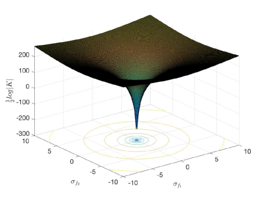
Figure 2: Gaussian process complexity surface obtained by the mixtures of two covariance functions (7) applied to 100 training instances from a Normal/AD separation task. Also note that maximizing $-\frac{1}{2}log|K|$ is equal to minimizing $\frac{1}{2}log|K|$ and additive noise $\sigma_{n}^{2}$ is missing is due to classification.

In regards to the types of basis kernels, we prefer homogeneous combinations and do not interleave different types of basis kernels in an attempt to simplify the problem. Otherwise, a heterogenous combination would require the normalization of kernel values since each kernel would have different output scales and the larger ones could dominate others. A basis kernel could cope with such a dominance by upscaling its outputs by taking on larger values for $\sigma_{f_{s}}$. However, we would not know whether the magnitude of $\sigma_{f_{s}}$ is due to the relevance of $\mathbf{x}_{is}$ to the problem or the competition between different kernel types.

3.2 On Efficiency and Generality

MKL-AsRD relaxes the requirement of ARD from evaluating the relations between observations at the granularity of individual dimensions to assessing the relations in subspaces and reduces the computational demands of the conventional approach. However, in the case of a large number of observations, the computational burden of MKL-AsRD could be dominated by kernel computations, especially if the kernels cannot be stored in main memory. In this regard, we assume that the entire computation takes place in memory, which also suits the small sample characteristics of our problem. Under our assumption, the efficiency of MKL-AsRD mainly depends on the granularity of feature bags. The smaller the feature bags, the larger will be the number of basis kernels and hyperparameters. As an extreme case, if all the feature bags are of cardinality of 1, each dimension gets assigned a basis kernel. In this extreme case, ARD and MKL-AsRD are equivalent in the sense that both are aimed at individual dimensions. However, depending on the numbers of hyperparameters associated with the basis kernels, the overall computation required by such an MKL-AsRD may be ridiculously higher than that required by ARD. Therefore, great care has to be taken in designing composite kernels and utilizing them for the discovery of relevant subspaces. At the other extreme, a big bag that can fit all features reduces the MKL problem to the traditional single kernel approach.

As demonstrated by the two extremes above, MKL-AsRD is a generalized solution for ARD. It can account for a wide range of possibilities at different levels of computational complexity. However, in practice, a trade-off has to be established between the full-fledged ARD and the single kernel learning. To this end, we heuristically define an upper bound for the total number of hyperparameters of a composite kernel as follows: $\sum_{s=1}^{S}h_{s}<D+1$, where $h_{s}$ is the number of hyperparameters associated with the $s$-th basis kernel, $D$ is the number of dimensions, and $D+1$ hyperparameters are required by ARD. For (24), $\forall s\in\left\{1,2,...,S\right\}h_{s}=2$, and an upper bound for the number of basis kernels is $S<(D+1)/2$. Due to the high dimensionality of neuroimaging data, we prefer $S\ll(D+1)/2$. Thus, MKL-AsRD is proposed as an approximate, but efficient, ARD solution.

3.3 Occam’s Razor

The principle of Occam’s razor states that given two models with the same generalization error, we should prefer the simpler one because the simplicity is a design goal [19]. Domingos [19] revised the razor that we should prefer the more comprehensible one, given two models with the same generalization error. While the comprehensibility is domain-dependent, in practice, we should constrain the model selection using domain-knowledge in order to promote simplicity and comprehensibility [19].

“Incorporating such constraints can simultaneously improve accuracy (by reducing the search needed to find an accurate model) and comprehensibility (by making the results of induction consistent with previous knowledge).” [19, p.5].

The razor motivates us to use the prior domain-knowledge regarding the inputs. Accordingly, we aim to avoid expensive search procedures required to find plausible feature bags and improve the classification performance and comprehensibility of the GP models.

3.3.1 Domain-Knowledge for Feature Bags

Recall that a kernel function represents our prior belief about the functions we wish to learn. Given a collection of 391 parametric images derived from PET scans and a taxonomy of 15,964 features that complies with the Talairach-Tournoux atlas, Ayhan et al. [5] handpicked certain regions of the brain containing characteristic patterns of AD based on domain-knowledge and showed that the use of domain-knowledge improves the prior specification even in case of the single kernel learning. Handpicking of cortical regions also resulted with significant computational gain, during both feature selection and training, and with no significant loss of classification performance [5]. Then, Ayhan et al. [7] investigated more flexible and sensible prior specifications via (24) and (25), which is absolutely desirable from the Bayesian perspective. Given the taxonomy of 15 anatomical regions, Ayhan et al. [7] specified anatomically motivated composite kernels and integrated information from many regions, each of which exhibits certain characteristics regarding the progression of AD.

Neuroimaging procedures capture the snapshots of the metabolic demands or activities of neurons in the brain into 3D volumes, the structures of which are known beforehand. For instance, an MRI scan is acquired one axial slice at a time (Figure 3). These slices are combined into a big volume of brain imagery, following certain processing steps, i.e., slice timing corrections [67, 3]. However, a taxonomy of voxels is not always available. In this regard, we consider the slices as feature bags, namely pseudo regions. In addition, we can use the spatial properties of voxels to come up with richer structural formations, e.g., cubes. One obvious advantage of using cubes is due to their ability to capture the 3D information about patterns in their proximity. A pattern of structural deformation that cuts across multiple slices may be captured by a single cube.

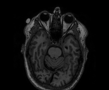
(a) Axial view (before)

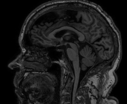
(b) Sagittal view (before)

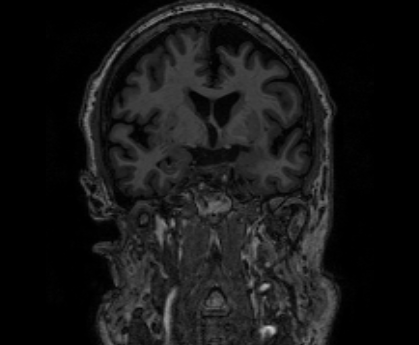
(c) Coronal view (before)

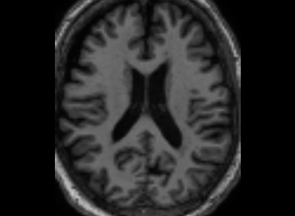
(d) Axial view (after)

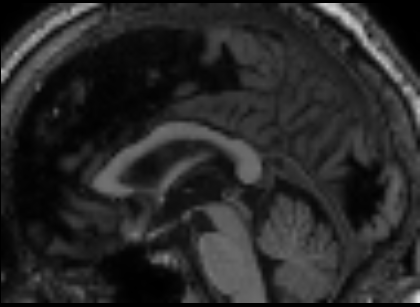
(e) Sagittal view (after)

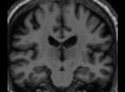
(f) Coronal view (after)

Figure 3: Visualization of an MRI scan from the AD class before and after normalization. Following the normalization, the dimensionality of neuroimages reduces from $170\times 256\times 256$ to $79\times 95\times 68$.

The structural information of MRI scans allows us to view the data from different perspectives. We wish to make an explicit use of the prior information and constrain the search for an appropriate arrangement of basis kernels to a particular setting defined with respect to slices and cubes. We hope to establish a proper trade-off for the supervised feature selection via MKL-AsRD.

4 Experiments

An SVM-based diagnostic method is competitive with or better than radiologists [38]. Therefore, we assume a typical SVM configuration as the baseline method and investigate the benefits of utilizing GPs for predictive modeling of AD. In this respect, our experimental setup is reminiscent of [7] which demonstrated the advantages of using GPs for the analysis of parametric images derived from PET scans. However, we use a larger collection of actual MRI scans, no taxonomy of voxels is present, and the dimensionality is much higher. Thus, the MRI data enable us to demonstrate the impact of MKL-AsRD under more complicated scenarios. Also, we provide a more detailed analysis of the diagnostic classification performance, including the predictive probabilities and multi-class classification results.

Initially, we compare the performances of two kernel machines on basis of the single kernel learning. Then, we aim to improve the diagnostic classification performance of the GP models via MKL-AsRD. We do not consider SVM under MKL settings, mainly due to the computational costs involved in MKL. The single kernel learning results also support us in so doing. In addition to benchmarking, we identify the prominent portions of the brain through data analysis and interpret the results in a manner consistent with the AD pathology. The impact of MKL-AsRD on predictive probabilities is of interest to us, as well.

In order to estimate the generalization performances of the specified algorithms, we apply 10-fold CV. Our performance metrics are classification accuracy, sensitivity, and specificity.

$$\text{Accuracy}=\frac{\text{True Pos. + True Neg.}}{\text{True Pos. + True Neg. + False Pos. + False Neg.}}$$

$$\text{Sensitivity}=\frac{\text{True Pos.}}{\text{True Pos. + False Neg.}}$$

$$\text{Specificity}=\frac{\text{True Neg.}}{\text{True Neg. + False Pos.}}$$

Sensitivity indicates our ability to recognize positive results, whereas specificity does it for negative results. For instance, given an AD patient, sensitivity is the probability that our classifier will assign the correct diagnosis. Specificity is the probability that our classifier will tell that the patient is healthy, given that he/she is, in fact, healthy. In medical diagnosis, the trade-off between these two measures are crucial. A highly sensitive test is valuable if there is a high penalty for missing positive cases [23]. “Sensitive tests are also helpful during the early stages of a diagnostic workup, when several diagnoses are being considered, to reduce the number of possibilities” [23, p.50]. On the other hand, highly specific tests are useful in reducing the risks as well as harm due to unnecessary procedures resulting from false positives [23]. Overall, it is desirable for a diagnostic test to achieve high sensitivity and specificity simultaneously. However, in practice, this may not be possible and one measure can be traded for the other [23]. In our experiments, we favor sensitivity because the risks involved in missing a positive case are usually greater than in misdiagnosing a healthy patient.

For binary classification tasks, we provide another measure: Area Under Curve (AUC). The AUC measure is obtained via Receiver Operating Characteristic (ROC) analysis and it summarizes the overall classification performance into one number. Based on the AUC scores, we compare the classification performances and test for significant differences.

For SVMs [14], we use a single linear kernel as well as the RBF kernel. A grid search is also performed using a fold of data. As a result, 80%, 10%, and 10% of data are used for training, validation, and testing, respectively. Note that we do not retrain SVMs after adding the validation set to the training set. Also, we consider the generation of probabilistic outputs along with class labels for each SVM configuration tested in single kernel learning scenarios. For the GP models [58], we use all the kernel functions described in Section 2.2 and Section 3.1. Since the GP models do not require validation sets, the training and test splits correspond to 90% and 10% of data. We fit a constant mean function to data and EP is used for inference, unless stated otherwise.

4.1 Data Acquisition

Data used in this study are from the Alzheimer’s Disease Neuroimaging Initiative (ADNI) (adni.loni.usc.edu). The ADNI was launched in 2003 as a public-private partnership, led by Principal Investigator Michael W. Weiner, MD. The primary goal of ADNI has been to test whether serial MRI, PET, other biological markers, and clinical and neuropsychological assessment can be combined to measure the progression of MCI and early AD.

4.2 Data Characteristics

Table 1 describes the demographics of the patients in the collection. There are three groups: Normal, MCI and AD. The MCI group is the largest and the dataset is skewed. In order to obtain a balanced dataset, 755 scans were randomly sampled without replacement from each group.

Table 1: Demographics of MRI data.

	Number of	Sex		Average	Number of
	Subjects	M	F	Age	MRI Scans
Normal	232	113	119	76.2	1278
MCI	411	267	114	75.5	2282
AD	200	103	97	76.0	755

4.3 Stereotactic Normalization

A raw MRI scan (Figure 3a-3c) consists of massive amounts of voxels and it needs to go through a preprocessing pipeline before analysis. The goals of preprocessing include the minimization of differences in brain size, shape and position, and hence the standardization of brain regions and tissue boundaries across subjects. Statistical Parametric Mapping (SPM) [3] is used to normalize the image data into an International Consortium for Brain Mapping (ICBM) template [29, 67]. Figure 3d-3f demonstrates the result of normalization. Note that no anatomical structure such as GM, white matter (WM) or cerebrospinal fluid (CSF) is extracted. Instead, the whole brain data is deliberately preserved because brain atrophy can be measured both in GM and WM [22]. We expect the machine learning software to figure out whatever is informative and determine the relevant portions of data.

4.4 Arrangement of the Basis Kernels

The number of basis kernels is essentially a hyperparameter for a given model. In the case of axial slices, the number is 68. However, if cubes are desired, it has to be determined according to user preferences. Given the dimensions of normalized MRI scans, the cube dimensions of $4\times 4\times 4$, $8\times 8\times 8$, $16\times 16\times 16$ and $32\times 32\times 32$ would result in 8160, 1080, 150, and 27 basis kernels, respectively, assuming that they were forbidden from overlapping. Due to the coarseness of the largest cube dimensions and excessive number of basis kernels induced by the smaller ones, we set the cube dimensions as $16\times 16\times 16$. This sweet spot not only leads to a significant saving on computational time but also helps us alleviate the potentially weaker consistency in the case of larger cube dimensions. Also note that, despite the fixed number and layout of kernels, we learn the kernel properties automatically from data, which is central to MKL.

4.5 Binary Classification Results

Table 2 shows the binary classification results. However, in many cases, it is difficult to discern the differences between performances. Since the numbers given in the table correspond to single points on the average ROC curves of the classifiers, we judge their performances by the AUC scores in Figure 4 while we keep the table for reference.

From Table 2 and Figure 4, we can tell that SVMs are fairly accurate. When we demand probabilistic outputs from SVMs, their performances are competitive with the basic configuration despite the use of smaller training sets. However, the generation of probabilities significantly complicates training. The differences between the performances of linear (LIN) and non-linear (RBF) SVMs indicate the non-linearity of the complex atrophy patterns. GPs tend to significantly outperform the baseline SVM, which is a linear one. Exceptions are those with a single SE covariance function or which used LA in slice-based MKL settings. Due to the quadratic form in the exponent of the SE covariance function, even the slightest change in a large number of input values easily causes the covariance between $f_{i}$ and $f_{j}$ to tend to zero. The same phenomenon was reported based on the experiments with PET data, as well [7]. However, SVMs with the RBF kernel are more robust to this situation, now. In our defense, the poor performance of such GP models can be rectified by the virtue of MKL-AsRD when the most relevant inputs are emphasized for the calculation of similarities (Figure 4a and Figure 4c). On the contrary, Figure 4b shows a case in which slice-based MKL-AsRD failed to recover from the catastrophe. In this case, the EP algorithm failed to complete during at least one iteration of CV, even though the remaining iterations resulted in performances that are comparable with other models’. Due to the instability concerns, we resorted to LA throughout CV. Evidently, LA failed to provide good estimates of mean and covariance. As a result, the performances are far from satisfying and the variation in the performance is larger compared with the others (Table 2, 22^nd row). Nevertheless, the use of cubes, instead of slices, remedies the situation.

Another observation to be made from Figure 4 is the competitiveness of the GP models equipped with linear covariance functions. Even a single function is quite satisfying in terms of classification performance. Considering the fewer number of hyperparameters and corresponding computational requirements, linear covariance function may be a natural choice for both single and multiple kernel learning scenarios. For those who want to make the most out of GP learning, the NN covariance function is also available.

Lastly, we did not expect the competitive performance demonstrated by a single linear covariance function before the experiments. Given the performances of linear SVMs, this seems counter intuitive. We speculate that it may be due to the algorithmic differences under the hood of the respective methodologies. On the bright side, GP models can outperform SVMs even in linear settings.

Table 2: The average generalization performances based on 10-fold CV. Standard deviations are given in parentheses. The highest average in each category is given in boldface with a preference for smaller deviation in cases of equality. GP^LA means that LA was used.

			Classifier	Accuracy	Sensitivity	Specificity
Normal vs. AD	Single Kernel		SVM LIN	89.20 (3.14)	89.60 (3.76)	88.80 (4.50)
			SVMprob LIN	89.20 (2.93)	89.87 (3.62)	88.53 (4.36)
			SVM RBF	90.60 (2.60)	90.80 (3.11)	90.40 (3.92)
			SVMprob RBF	89.87 (2.39)	90.67 (2.35)	89.07 (3.86)
			GP LIN	92.67 (1.57)	92.40 (2.67)	92.93 (1.89)
			GP SE	83.27 (2.02)	82.27 (4.31)	84.27 (3.31)
			GP NN	92.80 (1.47)	92.13 (2.70)	93.47 (1.60)
	MKL-AsRD	Slices	GP LIN	93.00 (2.07)	92.40 (3.50)	93.60 (1.86)
			GP SE	91.20 (2.79)	91.87 (3.23)	90.53 (3.95)
			GP NN	93.20 (2.43)	93.20 (3.74)	93.20 (2.39)
		Cubes	GP LIN	93.53 (1.34)	92.13 (2.91)	94.93 (2.25)
			GPLA SE	91.67 (2.04)	89.87 (3.28)	93.47 (2.31)
			GP NN	93.87 (1.72)	93.60 (2.73)	94.13 (2.89)
Normal vs. MCI	Single Kernel		SVM LIN	81.40 (3.93)	80.67 (3.78)	82.13 (5.15)
			SVMprob LIN	81.20 (3.72)	81.60 (4.25)	80.80 (4.45)
			SVM RBF	84.80 (2.77)	84.53 (3.78)	85.07 (4.39)
			SVMprob RBF	84.27 (2.83)	84.53 (3.57)	84.00 (3.98)
			GP LIN	86.13 (2.83)	84.00 (2.95)	88.27 (3.81)
			GP SE	72.13 (8.38)	76.00 (9.28)	68.27 (23.14)
			GP NN	86.20 (2.78)	84.13 (2.91)	88.27 (3.81)
	MKL-AsRD	Slices	GP LIN	87.40 (2.75)	86.53 (3.52)	88.27 (3.97)
			GPLA SE	72.27 (14.23)	73.60 (12.10)	70.93 (17.45)
			GP NN	88.07 (2.42)	86.93 (3.65)	89.20 (3.47)
		Cubes	GP LIN	89.60 (1.89)	88.93 (2.60)	90.27 (2.74)
			GPLA SE	87.27 (3.09)	85.20 (4.64)	89.33 (3.56)
			GP NN	89.93 (1.65)	89.73 (3.02)	90.13 (3.78)
MCI vs. AD	Single Kernel		SVM LIN	82.13 (3.73)	83.20 (4.92)	81.07 (4.52)
			SVMprob LIN	82.67 (3.40)	82.93 (4.98)	82.40 (4.65)
			SVM RBF	87.27 (2.25)	88.27 (3.86)	86.27 (4.03)
			SVMprob RBF	87.40 (2.28)	88.67 (4.13)	86.13 (3.68)
			GP LIN	88.80 (3.37)	91.07 (4.08)	86.53 (4.28)
			GP SE	80.27 (2.60)	79.33 (3.10)	81.20 (4.81)
			GP NN	88.87 (3.44)	90.80 (4.33)	86.93 (3.81)
	MKL-AsRD	Slices	GP LIN	89.40 (2.44)	92.00 (4.36)	86.80 (1.72)
			GPLA SE	88.00 (2.24)	88.67 (3.46)	87.33 (2.37)
			GP NN	88.73 (2.73)	91.20 (3.78)	86.27 (4.36)
		Cubes	GP LIN	88.87 (2.65)	90.53 (3.41)	87.20 (4.54)
			GPLA SE	87.53 (2.92)	88.40 (3.50)	86.67 (5.11)
			GP NN	89.13 (2.18)	90.13 (2.45)	88.13 (3.47)

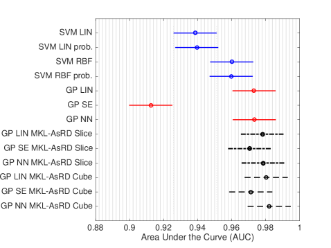
(a) Normal vs. AD

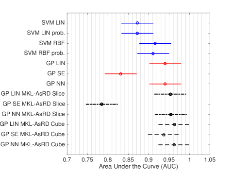
(b) Normal vs. MCI

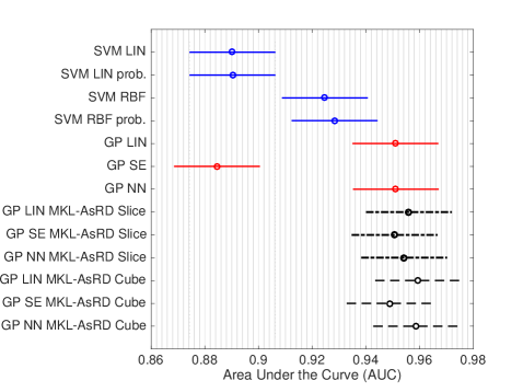
(c) MCI vs. AD

Figure 4: Average (mean) AUC results and comparison intervals for binary classification tasks. The confidence level is 95%. Two means are significantly different if their comparison intervals do not overlap.

4.5.1 Regions of Relevance and Comprehensibility

Figure 5 shows the relevant portions of brain imagery that are determined via MKL-AsRD. We consider the relevant slices and cubes as the regions of relevance (ROR). Since an anatomical taxonomy of them is not present, they are not exactly compatible with the known anatomical structures. However, Figure 5 shows that the models generally focus on the lower brain, where the AD pathology starts in and around the hippocampus and entorhinal cortex [72, 22]. Also note that the models are consistent in their preferences for the top regions in spite of the fundamental changes in their kernel configurations.

The patterns of atrophy due to AD are bilateral in spite of the greater impact on the left hemisphere [72]. The GP models with the cube-based MKL-AsRD capability better respond to the bilateral patterns of the AD pathology as it results in more connected structures in comparison with the slice-based configuration. (Figure 5).

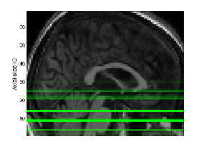
(a) Top 7 slices via GP LIN MKL-AsRD: 9,14,4,25,21,22,2

(b) Top 7 slices via GP SE MKL-AsRD: 14,9,24,8,10,23,11

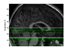
(c) Top 7 slices via GP NN MKL-AsRD: 14,30,4,9,26,22,15

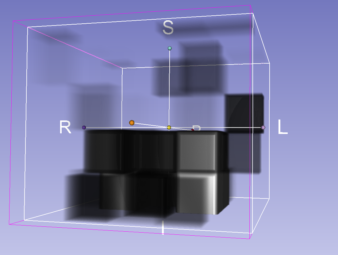
(d) Top 15 cubes via GP LIN MKL-AsRD: 46,41,106,47,71,107,42,77, 112,97,96,81,13, 116,87

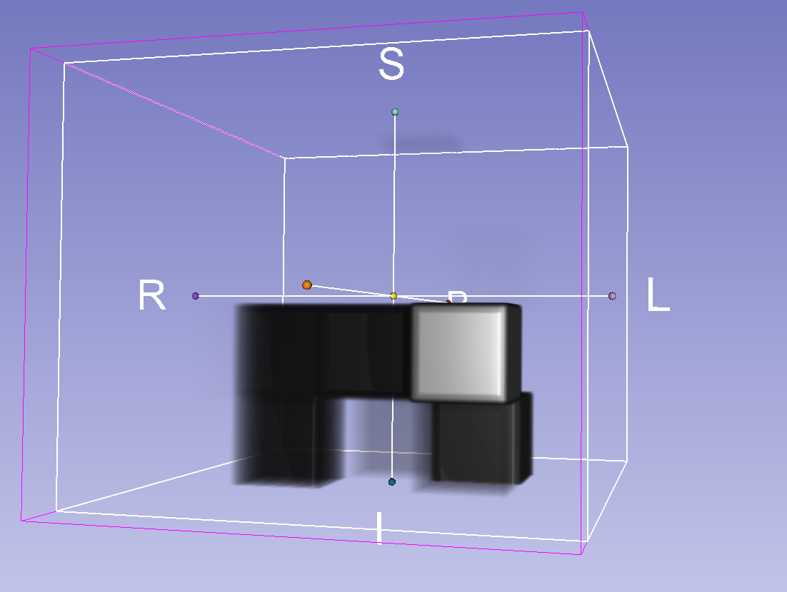
(e) Top 15 slices via GP SE MKL-AsRD: 47,41,77,107,106,46,71,97,52, 70,102,112,38, 43,103

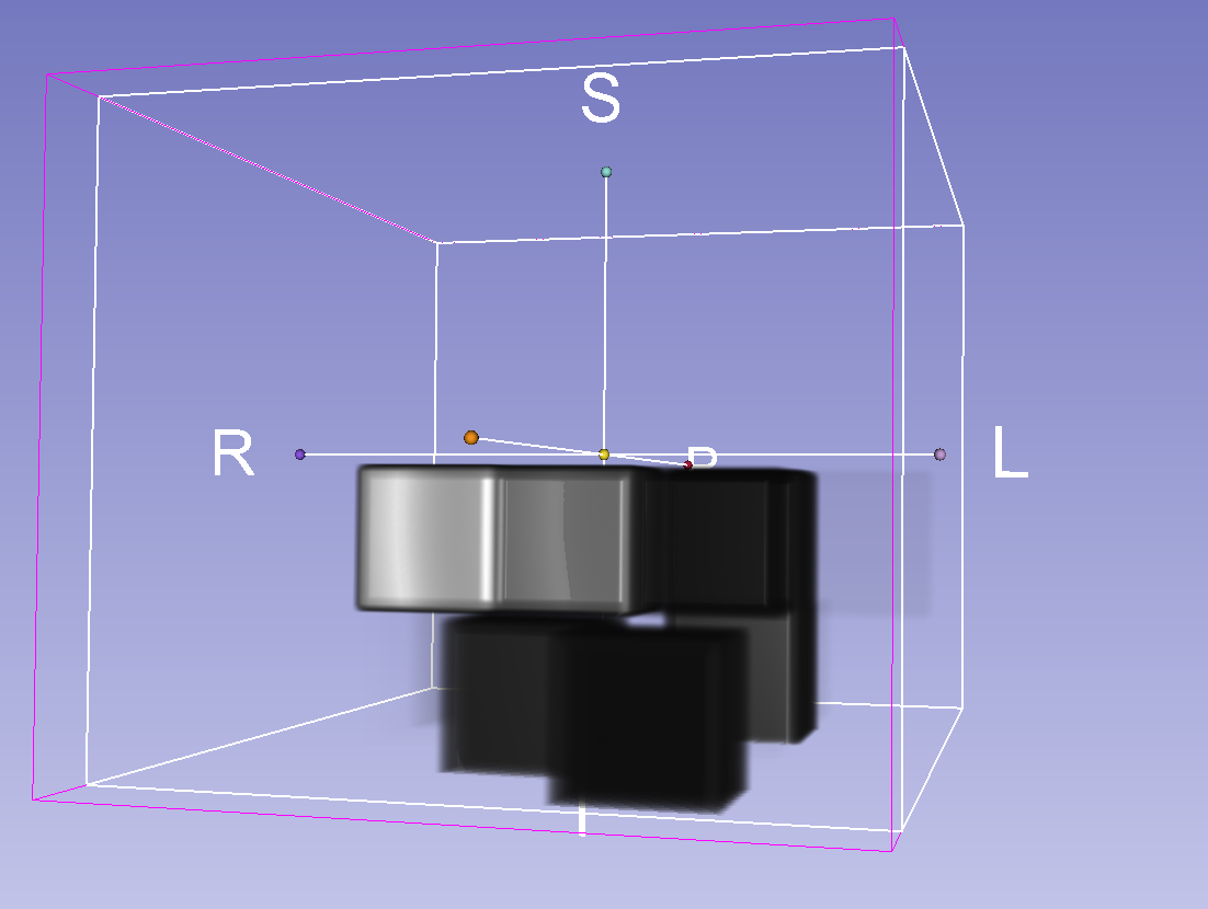
(f) Top 15 slices via GP NN MKL-AsRD: 107,77,41,42,81,56,47,97,101, 36,17,46,71, 106,112

Figure 5: Axial slices (top row) and cubes (bottom row) of relevance for Normal/AD classification. Relevance scores are determined based on 10-fold CV. For each CV iteration, the mixing weights are normalized separately. Then, they are accumulated over iterations. Note that the normalized weights are always less than or equal to 1. Thus, the relevance scores are between 0 and 10. In this scheme, a relevance score towards the high end of the spectrum indicates that the associated slice or cube has been emphasized many times during our experiments. On the other hand, a score from the low end means that the slice/cube was pretty much ignored due to its low relevance to the classification task at hand. In the top row, the brighter (greener) a slice is, the more relevant it is. Similarly, in the bottom row, the brighter (grayer) a cube is, the more relevant it is. Invisible cubes are considered irrelevant due to their relevance scores and hence not shown in the figures.

4.5.2 Predictive Probabilities

Figure 6 indicates that the GP models using a single SE covariance function tend to be overly cautious about their predictions. Even though the signs of predictions ($f_{*}$) are mostly correct, the predictive probabilities ($p_{*}$) are centered around 0.5 (Figure 6d). Such a conservative behavior can be associated with the underestimations of mean and covariance via LA [40]. But, it can happen due to the inappropriateness of the SE covariance function even if the EP algorithm is used for inference (Table 2, row 6). MKL-AsRD has a dramatic impact in this regard. The predictive probabilities are widespread and mostly closer to 0 or 1 (Figure 6e), which is desirable for confident decisions. Also, the average classification accuracy goes up by 7.93% as a result of MKL-AsRD. Another benefit of the MKL-AsRD is that it yields more confident models compared with the single kernel counterparts, even when LA is used for GP inference (Figure 6f). The first and last rows of Figure 6 show that MKL-AsRD improves the predictive probability distributions in cases of the linear and neural network covariance functions, as well. Not to mention, the choice of cubes leads to more confident models, in comparison with the slice-based configurations.

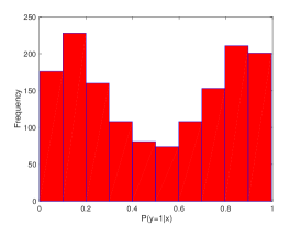
(a) GP LIN

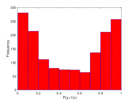
(b) GP LIN MKL-AsRD Slice

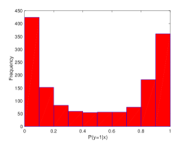
(c) GP LIN MKL-AsRD Cube

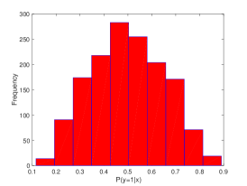
(d) GP SE

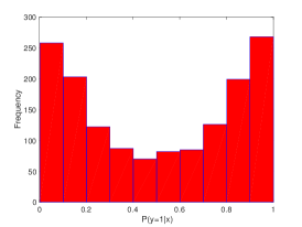
(e) GP SE MKL-AsRD Slice

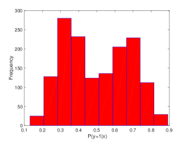
(f) GP SE MKL-AsRD Cube

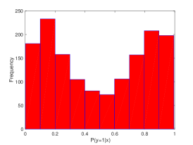
(g) GP NN

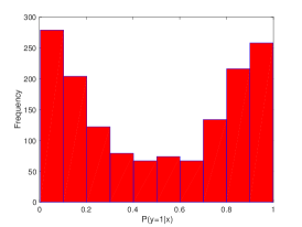
(h) GP NN MKL-AsRD Slice

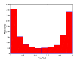
(i) GP NN MKL-AsRD Cube

Figure 6: Histograms of predictive probabilities via GP configurations for binary (Normal vs AD) classification task based on all test sets used during CV.

4.6 Multi-Class Classification Results

Dementia diagnosis is essentially a multi-class problem that can be decomposed into a series of binary classification problems. Probably the most popular schemes are One-vs-One (OVO) and One-vs-All (OVA). The OVO approach gives rise to $\binom{K}{2}$ classifiers, given $K$ classes. Each classifier separates a pair of classes. On the other hand, the OVA approach requires $K$ classifiers, each of which distinguishes a class from the others. OVO and OVA are competitive with other more complicated methods like single-machine schemes [60, 35]. Moreover, Rifkin and Klautau [60] reported that “a simple OVA scheme is as accurate as any other approach, assuming that the underlying binary classifiers are well-tuned regularized classifiers such as SVMs” [60, p.1]. Since we have established that the GP models are robust, high-performance classifiers, we use them for multi-class classification, adopting the OVA scheme.

Table 3 and Figure 7 present the multi-class classification performances of the previously described configurations. The trend is similar to those observed with the binary classification experiments. SVMs set a fairly high baseline for the GP models to match. As one would expect, the GP models with a single SE covariance function perform poorly. However, MKL-AsRD restores the modeling power of GPs, and two GP configurations, GP LIN MKL-AsRD Slice and GP NN MKL-AsRD Cube, significantly outperform the baseline SVM. The striking fact from Table 3 is that all classifiers struggle with the MCI class. The underlying classifiers trained for the discrimination of MCI from others always deliver low sensitivity but high specificity, which imposes a limitation on the multi-class accuracy. This phenomenon is also indicative of the large overlap between the MCI class and others, which has been reported by [22].

Table 3: Multi-class classification performances via OVA approach. For the GP models that utilize the SE covariance function, LA was used for inference. All other GP models were obtained via EP. Optimal parameters for the underlying binary SVMs were determined by a grid-search per SVM.

	Classifier	$+$ class	Binary Accuracy	Sensitivity	Specificity	Multi-class Accuracy
Single Kernel	SVM LIN	AD	89.42 (2.04)	86.13 (5.59)	91.07 (2.25)	80.22 (3.05)
		MCI	84.04 (3.03)	72.40 (4.49)	89.87 (3.62)
		Normal	86.98 (2.56)	82.13 (4.58)	89.40 (2.50)
	SVMprob LIN	AD	89.33 (1.93)	85.87 (5.70)	91.07 (2.52)	80.40 (3.48)
		MCI	83.96 (3.60)	72.93 (4.83)	89.47 (4.18)
		Normal	87.51 (2.91)	82.40 (4.57)	90.07 (2.69)
	SVM RBF	AD	90.89 (1.26)	88.53 (3.03)	92.07 (2.00)	83.02 (1.69)
		MCI	86.27 (2.18)	75.60 (5.11)	91.60 (2.81)
		Normal	88.89 (1.39)	84.93 (4.62)	90.87 (2.63)
	SVMprob RBF	AD	90.09 (1.72)	86.93 (4.44)	91.67 (1.76)	82.18 (3.11)
		MCI	85.16 (3.23)	75.60 (4.99)	89.93 (4.03)
		Normal	89.11 (2.08)	84.00 (4.91)	91.67 (2.71)
	GP LIN	AD	91.20 (1.58)	90.00 (4.37)	91.80 (1.44)	83.73 (1.38)
		MCI	86.84 (1.21)	73.33 (3.77)	93.60 (2.40)
		Normal	89.42 (1.27)	87.87 (4.46)	90.20 (2.74)
	GP SE	AD	81.42 (6.98)	76.93 (31.78)	83.67 (10.36)	64.44 (8.94)
		MCI	69.91 (8.38)	43.73 (31.99)	83.00 (18.55)
		Normal	77.56 (6.48)	72.67 (30.83)	80.00 (11.37)
	GP NN	AD	91.20 (1.58)	90.00 (4.37)	91.80 (1.44)	83.78 (1.38)
		MCI	86.89 (1.19)	73.47 (3.47)	93.60 (2.40)
		Normal	89.47 (1.31)	87.87 (4.46)	90.27 (2.69)
MKL-AsRD (Slices)	GP LIN	AD	91.91 (1.25)	90.27 (4.40)	92.73 (1.31)	85.64 (1.75)
		MCI	88.44 (1.15)	77.87 (3.40)	93.73 (2.36)
		Normal	90.93 (2.21)	88.80 (3.99)	92.00 (2.29)
	GP SE	AD	90.67 (2.67)	87.73 (5.99)	92.13 (1.96)	83.51 (3.16)
		MCI	86.98 (2.11)	74.67 (5.11)	93.13 (3.31)
		Normal	89.38 (2.05)	88.13 (5.05)	90.00 (2.39)
	GP NN	AD	91.73 (1.64)	90.40 (4.35)	92.40 (1.48)	85.24 (1.94)
		MCI	87.82 (1.28)	76.80 (4.45)	93.33 (2.37)
		Normal	90.93 (2.18)	88.53 (3.99)	92.13 (2.75)
MKL-AsRD (Cubes)	GP LIN	AD	91.38 (1.19)	90.40 (4.30)	91.87 (1.88)	85.38 (2.22)
		MCI	88.53 (2.67)	76.27 (7.24)	94.67 (2.24)
		Normal	90.84 (2.00)	89.47 (4.24)	91.53 (3.24)
	GP SE	AD	90.44 (1.74)	89.33 (4.91)	91.00 (2.58)	84.49 (2.64)
		MCI	87.33 (2.30)	74.67 (5.86)	93.67 (2.40)
		Normal	91.20 (2.48)	89.47 (4.28)	92.07 (3.42)
	GP NN	AD	92.67 (1.50)	90.80 (2.70)	93.60 (2.07)	86.71 (2.20)
		MCI	89.24 (2.50)	78.53 (6.17)	94.60 (1.87)
		Normal	91.51 (2.11)	90.80 (3.52)	91.87 (2.59)

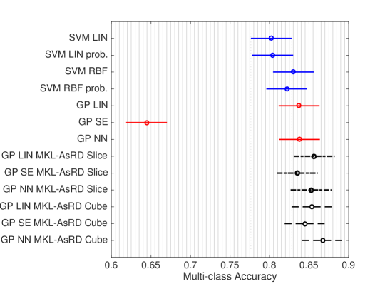
Figure 7: Average (mean) multi-class classification accuracies and comparison intervals. The confidence level is 95%. Two means are significantly different if their comparison intervals do not overlap.

5 Discussion

MKL generalizes the use of kernels and enables sophisticated extensions to the capabilities of kernel machines. A particular example is the multimodal classification, for which each modality is assigned its own kernel or kernels. Hinrichs et al. [31] showed the benefits of the multimodal classification by simultaneously using PET and MRI data. Since each imaging procedure captures different aspects of the underlying disease pathology, a linear combination of them is more informative for AD diagnosis [31]. As a result, the multimodal SVM outperforms the conventional one that uses only one modality at a time [31]. Zhang et al. [82] considered three modalities obtained from PET, MRI and CSF. Using an SVM, they, too, showed that MKL is superior to the single kernel learning. However, they used a grid search to determine the optimal mixing weights, which resulted in a secondary layer CV. The grid search and second level CV significantly complicates the model selection.

Young et al. [81] trained a GP classifier for the discrimination of AD from Normal based on the PET, MRI, CSF and apolipoprotein E (APOE) genotype data and used the model to predict the conversion from MCI to AD. They also compared the GP models to SVMs on the basis of their classification performances. Both kernel-machines were equipped with linear kernels and the GP models significantly outperformed the SVMs on the classification tasks involving multiple modalities [81]. In addition, they regarded the probabilistic outputs as risk scores for conversion to AD and approximated the continuum with respect to discrete stages of the disease. In a follow-up study, Young et al. [80] demonstrated the use of real-valued predictions for inferring the rate of conversion from MCI to AD. The elimination of discrete class labels increases the robustness to mislabeling. But, both the classification and regression approaches require data from multiple modalities. As a result, the final training set size is determined by the modality with the smallest number of examples [80]. The limitation on training data is a serious drawback that contaminates other multimodal approaches as well.

In our work, we exploit the power of MKL, without using multiple data modalities. Thus, we can use larger datasets in the first place. Secondly, we adopt a different perspective for the deployment of multiple kernels. Given a modality, we seek to discover new and implicitly accessible modalities from the given one. To better understand the analogy we make here, one can leave the mathematical sophistication aside and think that each kernel translates a portion of data into a feature space. Then, the features are combined into a very long vector that represents the input image from the given modality. Notice that our proposal does not exclude the possibility of the conventional multimodality since it can be adopted for each one separately. It is also notable that the previous studies on multi-modality adressed only the binary classification problems, i.e., Normal vs. AD, or Normal vs. MCI, and small scale kernel combinations, e.g., 3-4 kernels. In our experiments, we consider the multi-class classification as well as make use of larger scale kernel combinations, e.g., 150 kernels.

5.1 Representation Learning via Deep Architectures

Autoencoder (AE) is an unsupervised learning algorithm that automatically learns features from data. It is typically used to learn a compact, distributed representation of data [10]. Gupta et al. [29] used a sparse autoencoder (SAE) to obtain a set of bases from natural images. Using these natural image bases, they learned new and low dimensional representations of high dimensional MRI imagery by considering individual slices of 3D scans. The results obtained via the natural image bases are given in Table 4. In a follow-up study, Gupta et al. [30] investigated the advantages of the sparse, denoising and contractive AEs, over the basic AE. In terms of classification performance, even the basic AE is competitive with the sophisticated ones, given a large enough basis set [30]. However, the SAE enabled a new representation via only 100 bases, whereas the denoising, contractive and basic AEs required 200, 150 and 350 bases, respectively. The representation obtained by the SAE consisted of 61,200 features while the imagery contained 510,340 voxels [29, 30].

Table 4: Summary of the results obtained by MKL-AsRD, natural images via SAE [29], stacked AEs [45], and the combination of SAE with Convolutional neural network (CNN) [54]. The same MRI dataset was used by us, Gupta et al. [29], and Payan and Montana [54]. The numbers are the estimates of the generalization performances in terms of classification accuracy. A notable exception is the division of MCI into subclasses by Liu et al. [45]: nc-MCI and c-MCI. nc-MCI corresponds to the patients who have not converted to AD, whereas c-MCI patients did convert within 3 years from the initial screening.

	MKL-AsRD		SAE	Stacked AEs		SAE + CNN
Classes	2D	3D	Nat.Img.	MRI only	MRI+PET	2D	3D
Normal vs. AD	93.20%	93.87%	94.74%	82.59%	91.40%	95.39%	95.39%
Normal vs. MCI	88.07%	89.93%	86.35%	71.98%	82.10%	90.13%	92.11%
MCI vs. AD	89.40%	89.13%	88.10%	N/A		82.24%	86.84%
Normal, MCI, AD	85.64%	86.71%	85.00%			85.53%	89.47%
Normal, nc-MCI, c-MCI, AD				46.30%	53.79%
Representation	510,340		61,200	N/A		489,600	486,000
	voxels		features			features	features

Liu et al. [45] used stacked AEs to learn new representations from both MRI and PET scans simultaneously. The multimodal dataset consisted of only 331 instances. Also, instead of learning features directly from the neuroimagery, they extracted 83 ROIs from each modality and applied a feature engineering strategy to compute the first set of features. Then, some of the features were selected via the elastic net [84] on the basis of their discriminative power before being fed into the AEs. The extraction of predetermined ROIs resembles our selection of pseudo regions based on domain-knowledge. However, in our case, features are implicitly learned via kernel functions, parameters of which are also automatically tuned with respect to data. The use of hand-crafted features by Liu et al. [45] is at odds with the spirit of automated feature learning. The combined effect of the use of a small sample, predetermined ROIs, and hand-crafted features seems to have hindered their work (Table 4, shaded region).

Given the nature of neuroimages, 3D CNNs offer a great deal of opportunities in terms of obtaining sparsity and discovering many interesting relationships between inputs; however, moving from 2D to 3D significantly complicates the convolutional learning process [28]. Simply, 3D convolution requires many more filters in comparison with 2D convolution. Despite one can reduce the number of convolution filters by forbidding them from overlapping, extracting information from small and discrete patches is at odds with the need for the examination of complete brain imagery. Thankfully, Payan and Montana [54] proposed a deep architecture that consists of a SAE and a CNN followed by a feed-forward neural network. Basically, they used a SAE to learn 3D convolution filters. Then, these filters were used for feature extraction, which was followed by max-pooling and classification via a feed-forward neural network. Payan and Montana [54] also considered a similar feature extraction pipeline based on 2D filters. However, the 3D approach yields better performance as it better captures the spatial patterns of brain atrophy (Table 4, the rightmost column).

Table 4 also shows that MKL-AsRD is competitive with the aforementioned deep learning approaches to the computerized diagnosis of AD. Its accuracy for the separation of MCI and AD instances is particularly encouraging for further investigation of MKL-AsRD for early diagnosis and disease-modifying treatments. For instance, it can be pushed further into a feature learning pipeline in order to eliminate the use of predetermined ROIs (Section 6.1).

6 Conclusion

The proposed GP models are competitive with or better than the SVM which has been the workhorse of the multivariate predictive analysis of brain data. The added value of the GP models is that they readily provide probabilistic information regarding their predictions. Moreover, the models with MKL-AsRD capability respond to the patterns of AD pathology and emphasize the prominent anatomical regions and their proximities for accurate staging of AD. Last but not least, these models can compete with deep learning solutions under similar settings. Supporting the view of Klöppel et al. [38], we consider them highly practical. Carefully trained and validated models can be deployed at neuroimaging centers in order to speed up the diagnostic processes with no compromise of accuracy and support accurate decision-making based on probabilistic reasoning in cases where there is a lack of access to an experienced physician.

6.1 Future Directions

Deep learning sets a definitive direction, considering its impressive successes over a plethora of applications  [33, 34, 61, 42, 39, 66, 20, 24]. Deep learning is dominated by neural networks that consist of multiple layers of many hidden units for higher levels of representation. Given that neuroimages are big, naive approaches end in rapid memory blow-up as well as high computation time. In this regard, it is common for deep learning applications to extract information from small patches of larger images [42, 39, 29, 30]. Convolution via patches is also a key for learning representations [43, 66, 20, 24]. However, 3D convolution is a complicated process due to the volumes of neuroimages. In this regard, as an immediate extension, we would like to combine deep learning methods with the GP models proposed as biomarkers. Our goal is to learn new representations of neuroimages from the most relevant portions of data. Considering that a structure observed in brain imagery is dictated by an anatomical as well as functional organization [17], we expect to outperform the slice-based representations [29, 30, 54] by better exploiting the spatial relationships in data. Also, we will eliminate the need for 3D convolution by learning representations from all RORs at once. Last but not least, this approach can be easily extended to a multimodal scenario, under which multiple data types, e.g., PET and MRI, will be used simultaneously.

Acknowledgments

Data collection and sharing for this project was funded by the ADNI (National Institutes of Health (NIH) Grant U01 AG024904) and DOD ADNI (Department of Defense award number W81XWH-12-2-0012). ADNI is funded by the NIA, the National Institute of Biomedical Imaging and Bioengineering, and through generous contributions from the following: AbbVie, AA; Alzheimer’s Drug Discovery Foundation; Araclon Biotech; BioClinica, Inc.; Biogen; Bristol-Myers Squibb Company; CereSpir, Inc.; Eisai Inc.; Elan Pharmaceuticals, Inc.; Eli Lilly and Company; EuroImmun; F. Hoffmann-La Roche Ltd and its affiliated company Genentech, Inc.; Fujirebio; GE Healthcare; IXICO Ltd.; Janssen Alzheimer Immunotherapy Research & Development, LLC.; Johnson & Johnson Pharmaceutical Research & Development LLC.; Lumosity; Lundbeck; Merck & Co., Inc.; Meso Scale Diagnostics, LLC.; NeuroRx Research; Neurotrack Technologies; Novartis Pharmaceuticals Corporation; Pfizer Inc.; Piramal Imaging; Servier; Takeda Pharmaceutical Company; and Transition Therapeutics. The Canadian Institutes of Health Research is providing funds to support ADNI clinical sites in Canada. Private sector contributions are facilitated by the Foundation for the NIH (www.fnih.org). The grantee organization is the Northern California Institute for Research and Education, and the study is coordinated by the Alzheimer’s Disease Cooperative Study at the University of California, San Diego. ADNI data are disseminated by the Laboratory for Neuro Imaging at the University of Southern California.

In preparation of this article, we used portions of text from our earlier work: [5],[7], and [29]. Specifically, Section 2.2, 2.3 and 3.3 are extended from the corresponding sections of our earlier work [5, 7]. The extended material offers a comprehensive review of the GP learning and a comparison of the GP classifier with SVM. Given that our work relies on the principle of Occam’s razor, we reiterated the principle by using text from [5] and elaborated on the idea towards MKL-AsRD. This study also shares data with [29] but we test different hypotheses and our experimental setup is unique to us. We thank our collaborators for their contribution that led us to this study.

References

- Alzheimer’s Association [2017] Alzheimer’s Association. 2017 Alzheimer’s disease facts and figures. Alzheimer’s & Dementia, 13(4):325 – 373, 2017. ISSN 1552-5260. doi: https://doi.org/10.1016/j.jalz.2017.02.001. URL http://www.sciencedirect.com/science/article/pii/S1552526017300511.
- Archambeau and Bach [2011] C. Archambeau and F. Bach. Multiple Gaussian process models. arXiv preprint arXiv:1110.5238, 2011.
- Ashburner et al. [2010] J. Ashburner, G. Barnes, C. Chen, J. Daunizeau, G. Flandin, K. Friston, D. Gitelman, S. Kiebel, J. Kilner, V. Litvak, R. Moran, W. Penny, K. Stephan, D. Gitelman, R. Henson, C. Hutton, V. Glauche, J. Mattout, and C. Phillips. SPM8 manual, July 2010.
- Ayhan et al. [2010] M. S. Ayhan, R. G. Benton, V. V. Raghavan, and S. Choubey. Exploitation of 3D stereotactic surface projection for automated classification of Alzheimer’s disease according to dementia levels. In 2010 IEEE International Conference on Bioinformatics and Biomedicine (BIBM), pages 516–519. IEEE, 2010.
- Ayhan et al. [2012] M. S. Ayhan, R. G. Benton, S. Choubey, and V. V. Raghavan. Utilization of domain-knowledge for simplicity and comprehensibility in predictive modeling of Alzheimer’s disease. In Proceedings of the 2012 IEEE International Conference on Bioinformatics and Biomedicine Workshops (BIBMW), BIBMW ’12, pages 265–272, 2012. ISBN 978-1-4673-2746-6.
- Ayhan et al. [2013a] M. S. Ayhan, R. G. Benton, V. V. Raghavan, and S. Choubey. Exploitation of 3D stereotactic surface projection for predictive modelling of Alzheimer’s disease. Int. J. Data Min. Bioinformatics, 7(2):146–165, Apr. 2013a. ISSN 1748-5673.
- Ayhan et al. [2013b] M. S. Ayhan, R. G. Benton, V. V. Raghavan, and S. Choubey. Composite kernels for automatic relevance determination in computerized diagnosis of alzheimer’s disease. In International Conference on Brain and Health Informatics, pages 126–137. Springer, 2013b.
- Bach [2008] F. R. Bach. Consistency of the group lasso and multiple kernel learning. J. Mach. Learn. Res., 9:1179–1225, June 2008. ISSN 1532-4435. URL http://dl.acm.org/citation.cfm?id=1390681.1390721.
- Bach et al. [2004] F. R. Bach, G. R. G. Lanckriet, and M. I. Jordan. Multiple kernel learning, conic duality, and the SMO algorithm. In Proceedings of the Twenty-first International Conference on Machine Learning, ICML ’04, pages 6–13, 2004. ISBN 1-58113-838-5.
- Bengio [2009] Y. Bengio. Learning deep architectures for AI. Found. Trends Mach. Learn., 2(1):1–127, Jan. 2009. ISSN 1935-8237.
- Bishop and Tipping [2003] C. M. Bishop and M. E. Tipping. Bayesian regression and classification. In J. Suykens, G. Horvath, S. Basu, C. Micchelli, and J. Vandewalle, editors, Advances in Learning Theory: Methods, Models and Applications, volume 190 of NATO Science Series III: Computer and Systems Sciences, pages 267–285. IOS Press, 2003.
- Candela [2004] J. Q. Candela. Learning with uncertainty-Gaussian processes and relevance vector machines. PhD thesis, Technical University of Denmark, 2004.
- Caruana [1998] R. Caruana. Multitask Learning. In Learning to Learn, pages 95–133. Springer, 1998.
- Chang and Lin [2011] C.-C. Chang and C.-J. Lin. LIBSVM: A library for support vector machines. ACM Trans. Intell. Syst. Technol., 2(3):27:1–27:27, May 2011. ISSN 2157-6904.
- Christoudias et al. [2009] M. Christoudias, R. Urtasun, and T. Darrell. Bayesian localized multiple kernel learning. Technical report, University of California at Berkeley, 2009.
- Cortes et al. [2009] C. Cortes, M. Mohri, and A. Rostamizadeh. L2 regularization for learning kernels. In Proceedings of the Twenty-Fifth Conference on Uncertainty in Artificial Intelligence, UAI ’09, pages 109–116, 2009. ISBN 978-0-9749039-5-8.
- Cuingnet et al. [2013] R. Cuingnet, J. A. Glaunes, M. Chupin, H. Benali, and O. Colliot. Spatial and anatomical regularization of svm: a general framework for neuroimaging data. Pattern Analysis and Machine Intelligence, IEEE Transactions on, 35(3):682–696, 2013.
- Damianou and Lawrence [2013] A. Damianou and N. Lawrence. Deep Gaussian processes. In Proceedings of the Sixteenth International Conference on Artificial Intelligence and Statistics (AISTATS 2013), pages 207–215, 2013.
- Domingos [1998] P. Domingos. Occam’s two razors: The sharp and the blunt. In In Proceedings of the Fourth International Conference on Knowledge Discovery and Data Mining, pages 37–43. AAAI Press, 1998.
- Dosovitskiy et al. [2014] A. Dosovitskiy, J. T. Springenberg, and T. Brox. Learning to generate chairs with convolutional neural networks. arXiv preprint arXiv:1411.5928, 2014.
- Duvenaud et al. [2011] D. K. Duvenaud, H. Nickisch, and C. E. Rasmussen. Additive Gaussian processes. In J. Shawe-Taylor, R. Zemel, P. Bartlett, F. Pereira, and K. Weinberger, editors, Advances in Neural Information Processing Systems 24, pages 226–234. 2011.
- Fan et al. [2008] Y. Fan, N. Batmanghelich, C. M. Clark, and C. Davatzikos. Spatial patterns of brain atrophy in MCI patients, identified via high-dimensional pattern classification, predict subsequent cognitive decline. NeuroImage, 39(4):1731–1743, 2008. ISSN 1053-8119. doi: http://dx.doi.org/10.1016/j.neuroimage.2007.10.031.
- [23] R. Fletcher, S. Fletcher, and G. Fletcher. Clinical Epidemiology: The Essentials. M - Medicine Series. ISBN 9781451144475.
- Flynn et al. [2015] J. Flynn, I. Neulander, J. Philbin, and N. Snavely. Deepstereo: Learning to predict new views from the world’s imagery. CoRR, abs/1506.06825, 2015.
- Gönen [2012] M. Gönen. Bayesian efficient multiple kernel learning. In J. Langford and J. Pineau, editors, Proceedings of the 29th International Conference on Machine Learning (ICML-12), ICML ’12, pages 1–8, New York, NY, USA, July 2012. Omnipress. ISBN 978-1-4503-1285-1.
- Gönen and Alpaydin [2011] M. Gönen and E. Alpaydin. Multiple kernel learning algorithms. J. Mach. Learn. Res., 12:2211–2268, July 2011. ISSN 1532-4435.
- Gonnella et al. [1984] J. S. Gonnella, M. C. Hornbrook, and D. Z. Louis. Staging of disease: A case-mix measurement. JAMA, 251(5):637–644, 1984. doi: 10.1001/jama.1984.03340290051021.
- Graham [2015] B. Graham. Sparse 3d convolutional neural networks. arXiv preprint arXiv:1505.02890, 2015.
- Gupta et al. [2013a] A. Gupta, M. S. Ayhan, and A. S. Maida. Natural image bases to represent neuroimaging data. In Proceedings of the 30th International Conference on Machine Learning (ICML-13), ICML’13, June 2013a.
- Gupta et al. [2013b] A. Gupta, M. S. Ayhan, and A. S. Maida. Evaluation of autoencoders for bases to represent neuroimaging data. In NIPS 2013 Workshop on Machine Learning and Interpretation in NeuroImaging, December 2013b.
- Hinrichs et al. [2009] C. Hinrichs, V. Singh, G. Xu, and S. Johnson. Mkl for robust multi-modality ad classification. In Medical Image Computing and Computer-Assisted Intervention–MICCAI 2009, pages 786–794. Springer, 2009.
- Hinrichs et al. [2012] C. Hinrichs, V. Singh, J. Peng, and S. C. Johnson. Q-MKL: Matrix-induced regularization in multi-kernel learning with applications to neuroimaging. In NIPS, pages 1430–1438, 2012.
- Hinton and Salakhutdinov [2006] G. E. Hinton and R. R. Salakhutdinov. Reducing the dimensionality of data with neural networks. Science, 313(5786):504–507, 2006.
- Hinton et al. [2006] G. E. Hinton, S. Osindero, and Y.-W. Teh. A fast learning algorithm for deep belief nets. Neural Comput., 18(7):1527–1554, July 2006. ISSN 0899-7667.
- Huang et al. [2006] T.-K. Huang, R. C. Weng, and C.-J. Lin. Generalized Bradley-Terry models and multi-class probability estimates. J. Mach. Learn. Res., 7:85–115, Dec. 2006. ISSN 1532-4435.
- Hyvärinen et al. [2009] A. Hyvärinen, J. Hurri, and P. O. Hoyer. Natural Image Statistics: A Probabilistic Approach to Early Computational Vision. Springer Publishing Company, Incorporated, 1st edition, 2009. ISBN 1848824904, 9781848824904.
- Imabayashi et al. [2004] E. Imabayashi, H. Matsuda, T. Asada, T. Ohnishi, S. Sakamoto, S. Nakano, and T. Inoue. Superiority of 3-dimensional stereotactic surface projection analysis over visual inspection in discrimination of patients with very early Alzheimer’s disease from controls using brain perfusion SPECT. Journal of Nuclear Medicine, 45(9):1450–1457, 2004.
- Klöppel et al. [2008] S. Klöppel, C. M. Stonnington, J. Barnes, F. Chen, C. Chu, C. D. Good, I. Mader, L. A. Mitchell, A. C. Patel, C. C. Roberts, et al. Accuracy of dementia diagnosis–a direct comparison between radiologists and a computerized method. Brain, 131(11):2969–2974, 2008.
- Krizhevsky et al. [2012] A. Krizhevsky, I. Sutskever, and G. E. Hinton. ImageNet classification with deep convolutional neural networks. In NIPS, volume 1, page 4, 2012.
- Kuss and Rasmussen [2005] M. Kuss and C. E. Rasmussen. Assessing approximate inference for binary Gaussian process classification. The Journal of Machine Learning Research, 6:1679–1704, 2005.
- Lanckriet et al. [2004] G. R. G. Lanckriet, N. Cristianini, P. Bartlett, L. E. Ghaoui, and M. I. Jordan. Learning the kernel matrix with semidefinite programming. J. Mach. Learn. Res., 5:27–72, Dec. 2004. ISSN 1532-4435.
- Le et al. [2011] Q. V. Le, R. Monga, M. Devin, G. Corrado, K. Chen, J. D. Marc’Aurelio Ranzato, and A. Y. Ng. Building high-level features using large scale unsupervised learning. arXiv preprint arXiv:1112.6209, 2011.
- LeCun et al. [1998] Y. LeCun, L. Bottou, Y. Bengio, and P. Haffner. Gradient-based learning applied to document recognition. Proceedings of the IEEE, 86(11):2278–2324, 1998.
- Lin et al. [2007] H.-T. Lin, C.-J. Lin, and R. C. Weng. A note on Platt’s probabilistic outputs for support vector machines. Mach. Learn., 68(3):267–276, Oct. 2007. ISSN 0885-6125.
- Liu et al. [2015] S. Liu, S. Liu, W. Cai, H. Che, S. Pujol, R. Kikinis, D. Feng, and M. J. Fulham. Multimodal neuroimaging feature learning for multiclass diagnosis of Alzheimer’s disease. Biomedical Engineering, IEEE Transactions on, 62(4):1132–1140, 2015.
- MacKay [1996] D. J. MacKay. Bayesian methods for backpropagation networks. In Models of neural networks III, pages 211–254. Springer, 1996.
- Matsuda [2007] H. Matsuda. Role of neuroimaging in Alzheimer’s disease, with emphasis on brain perfusion spect. Journal of Nuclear Medicine, 48(8):1289–1300, 2007.
- Melkumyan and Ramos [2011] A. Melkumyan and F. Ramos. Multi-kernel Gaussian processes. In IJCAI Proceedings-International Joint Conference on Artificial Intelligence, volume 22, page 1408, 2011.
- Mercer [1909] J. Mercer. Functions of positive and negative type, and their connection with the theory of integral equations. Philosophical Transactions of the Royal Society of London. Series A, Containing Papers of a Mathematical or Physical Character, 209:pp. 415–446, 1909. ISSN 02643952.
- Minka [2001] T. P. Minka. A family of algorithms for approximate Bayesian inference. PhD thesis, Massachusetts Institute of Technology, 2001.
- Minoshima et al. [1995] S. Minoshima, K. A. Frey, R. A. Koeppe, N. L. Foster, and D. E. Kuhl. A diagnostic approach in Alzheimer’s disease using three-dimensional stereotactic surface projections of fluorine-18-FDG PET. Journal of Nuclear Medicine, 36(7):1238–1248, 1995.
- Neal [1996] R. M. Neal. Bayesian Learning for Neural Networks. Springer-Verlag New York, Inc., Secaucus, NJ, USA, 1996. ISBN 0387947248.
- Nickisch and Rasmussen [2008] H. Nickisch and C. E. Rasmussen. Approximations for binary Gaussian process classification. Journal of Machine Learning Research, 9:2035–2078, 2008.
- Payan and Montana [2015] A. Payan and G. Montana. Predicting Alzheimer’s disease: a neuroimaging study with 3D convolutional neural networks. arXiv preprint arXiv:1502.02506, 2015.
- Petersen et al. [2001] R. C. Petersen, R. Doody, A. Kurz, R. C. Mohs, J. C. Morris, P. V. Rabins, K. Ritchie, M. Rossor, L. Thal, and B. Winblad. Current concepts in mild cognitive impairment. Archives of Neurology, 58(12):1985, 2001.
- Platt [1999] J. C. Platt. Probabilistic outputs for support vector machines and comparisons to regularized likelihood methods. Advances in Large Margin Classifiers, 10(3):61–74, 1999.
- Rakotomamonjy et al. [2008] A. Rakotomamonjy, F. R. Bach, S. Canu, and Y. Grandvalet. SimpleMKL. Journal of Machine Learning Research, 9:2491–2521, Nov. 2008.
- Rasmussen and Nickisch [2010] C. E. Rasmussen and H. Nickisch. Gaussian Processes for Machine Learning (GPML) toolbox. The Journal of Machine Learning Research, 9999:3011–3015, 2010.
- Rasmussen and Williams [2005] C. E. Rasmussen and C. K. I. Williams. Gaussian Processes for Machine Learning (Adaptive Computation and Machine Learning). The MIT Press, 2005. ISBN 026218253X.
- Rifkin and Klautau [2004] R. Rifkin and A. Klautau. In defense of one-vs-all classification. J. Mach. Learn. Res., 5:101–141, Dec. 2004. ISSN 1532-4435.
- Salakhutdinov et al. [2007] R. Salakhutdinov, A. Mnih, and G. Hinton. Restricted boltzmann machines for collaborative filtering. In Proceedings of the 24th international conference on Machine learning, pages 791–798. ACM, 2007.
- Schölkopf and Smola [2001] B. Schölkopf and A. J. Smola. Learning with Kernels: Support Vector Machines, Regularization, Optimization, and Beyond. MIT Press, Cambridge, MA, USA, 2001. ISBN 0262194759.
- Snelson and Ghahramani [2006a] E. Snelson and Z. Ghahramani. Sparse Gaussian processes using pseudo-inputs. In Advances in Neural Information Processing Systems 18, pages 1257–1264. MIT press, 2006a.
- Snelson and Ghahramani [2006b] E. Snelson and Z. Ghahramani. Variable noise and dimensionality reduction for sparse Gaussian processes. In Proceedings of the Twenty-Second Conference Annual Conference on Uncertainty in Artificial Intelligence (UAI-06), pages 461–468, Arlington, Virginia, 2006b. AUAI Press.
- Sonnenburg et al. [2006] S. Sonnenburg, G. Rätsch, C. Schäfer, and B. Schölkopf. Large scale multiple kernel learning. J. Mach. Learn. Res., 7:1531–1565, Dec. 2006. ISSN 1532-4435.
- Szegedy et al. [2014] C. Szegedy, W. Liu, Y. Jia, P. Sermanet, S. Reed, D. Anguelov, D. Erhan, V. Vanhoucke, and A. Rabinovich. Going deeper with convolutions. arXiv preprint arXiv:1409.4842, 2014.
- Thatcher [1994] R. W. Thatcher. Functional neuroimaging: technical foundations. Academic Press, 1994. ISBN 9780126858457.
- Tibshirani [1996] R. Tibshirani. Regression shrinkage and selection via the lasso. Journal of the Royal Statistical Society. Series B (Methodological), pages 267–288, 1996.
- Tipping [2001] M. E. Tipping. Sparse Bayesian learning and the relevance vector machine. J. Mach. Learn. Res., 1:211–244, Sept. 2001. ISSN 1532-4435.
- Tu [2007] Z. Tu. Learning generative models via discriminative approaches. In Computer Vision and Pattern Recognition, 2007. CVPR’07. IEEE Conference on, pages 1–8. IEEE, 2007.
- Vapnik [1995] V. N. Vapnik. The nature of statistical learning theory. Springer-Verlag New York, Inc., New York, NY, USA, 1995. ISBN 0-387-94559-8.
- Whitwell et al. [2007] J. L. Whitwell, S. A. Przybelski, S. D. Weigand, D. S. Knopman, B. F. Boeve, R. C. Petersen, and C. R. Jack. 3D maps from multiple MRI illustrate changing atrophy patterns as subjects progress from mild cognitive impairment to Alzheimer’s disease. Brain, 130(7):1777–1786, 2007.
- WHO International Programme on Chemical Safety [2001] WHO International Programme on Chemical Safety. Biomarkers in risk assessment: Validity and validation. World Health Organization International Programme on Chemical Safety, Environmental Health Criteria 155, 2001.
- Wiering et al. [2013] M. Wiering, M. Van der Ree, M. Embrechts, M. Stollenga, A. Meijster, A. Nolte, and L. Schomaker. The Neural Support Vector Machine. In The 25th Benelux Artificial Intelligence Conference (BNAIC). IEEE, 2013.
- Williams and Barber [1998] C. K. I. Williams and D. Barber. Bayesian classification with Gaussian processes. IEEE Trans. Pattern Anal. Mach. Intell., 20(12):1342–1351, Dec. 1998. ISSN 0162-8828.
- Wipf and Nagarajan [2007] D. P. Wipf and S. S. Nagarajan. A new view of automatic relevance determination. In Advances in Neural Information Processing Systems, pages 1625–1632, 2007.
- Wu et al. [2004] T.-F. Wu, C.-J. Lin, and R. C. Weng. Probability estimates for multi-class classification by pairwise coupling. J. Mach. Learn. Res., 5:975–1005, Dec. 2004. ISSN 1532-4435.
- Xu et al. [2009] H. Xu, C. Caramanis, and S. Mannor. Robustness and regularization of Support Vector Machines. The Journal of Machine Learning Research, 10:1485–1510, 2009.
- Yang et al. [2011] W. Yang, R. L. M. Lui, J. H. Gao, T. F. Chan, S. Yau, R. A. Sperling, and X. Huang. Independent component analysis-based classification of Alzheimer’s Disease MRI Data. Journal of Alzheimer’s Disease, 24(4):775–783, 2011.
- Young et al. [2013a] J. Young, M. Modat, M. J. Cardoso, J. Ashburner, and S. Ourselin. An oblique approach to prediction of conversion to Alzheimer’s disease with multikernel Gaussian processes. In NIPS 2013 Workshop on Machine Learning and Interpretation in NeuroImaging, December 2013a.
- Young et al. [2013b] J. Young, M. Modat, M. J. Cardoso, A. Mendelson, D. Cash, and S. Ourselin. Accurate multimodal probabilistic prediction of conversion to Alzheimer’s disease in patients with mild cognitive impairment. NeuroImage: Clinical, 2(0):735–745, 2013b. ISSN 2213-1582. doi: http://dx.doi.org/10.1016/j.nicl.2013.05.004.
- Zhang et al. [2011] D. Zhang, Y. Wang, L. Zhou, H. Yuan, and D. Shen. Multimodal classification of Alzheimer’s disease and mild cognitive impairment. Neuroimage, 55(3):856–867, 2011.
- Zhao and Yu [2006] P. Zhao and B. Yu. On model selection consistency of lasso. J. Mach. Learn. Res., 7:2541–2563, Dec. 2006. ISSN 1532-4435. URL http://dl.acm.org/citation.cfm?id=1248547.1248637.
- Zou and Hastie [2005] H. Zou and T. Hastie. Regularization and variable selection via the elastic net. Journal of the Royal Statistical Society: Series B (Statistical Methodology), 67(2):301–320, 2005.