Higher-order meshing of implicit geometries—part II:
Approximations on manifolds

Abstract

A new concept for the higher-order accurate approximation of partial differential equations on manifolds is proposed where a surface mesh composed by higher-order elements is automatically generated based on level-set data. Thereby, it enables a completely automatic workflow from the geometric description to the numerical analysis without any user-intervention. A master level-set function defines the shape of the manifold through its zero-isosurface which is then restricted to a finite domain by additional level-set functions. It is ensured that the surface elements are sufficiently continuous and shape regular which is achieved by manipulating the background mesh. The numerical results show that optimal convergence rates are obtained with a moderate increase in the condition number compared to handcrafted surface meshes.

Keywords: higher-order FEM, manifold, surface PDEs, level-set method

1 Introduction

Many challenging applications in engineering and natural sciences are characterized by physical phenomena taking place on curved surfaces in the three-dimensional space. There are numerous examples for transport and flow phenomena on biomembranes or bubble surfaces [26, 39]. Examples in structures are membranes and shells [7, 3]. Phenomena on surfaces may also be coupled to processes in the surrounding volume such as in surfactant transport, hydraulic fracturing, reinforced structures etc. As an additional challenge, the surfaces may be moving [18, 40, 22], i.e. the domain of interest changes. The modeling of such phenomena naturally leads to boundary value problems where partial differential equations are formulated on manifolds. For the solution of such models, customized numerical methods are needed.

The first application of the finite element method for the solution of the Laplace-Beltrami operator on manifolds is reported in 1988 by Dziuk [17]. Since then, the topic has attracted a tremendous research interest leading to a variety of numerical methods for PDEs on surfaces existing today, see [20] for an overview. The most straightforward approach is to generate surface meshes on the manifold and extend the finite element method in a natural way using tangential differential calculus. That is, standard gradients of the planar two-dimensional case are replaced by surface gradients on the manifold. It is interesting to note that this approach has been chosen from the beginning in the simulation of transport phenomena, e.g. [2, 1, 16, 20]. However, for the modeling of membranes and shells, a less intuitive path using local coordinate systems and Christoffel symbols is standard since a long time [7, 3]. It is rather recent that these models have been recasted in the frame of global tangential operators [10, 11, 28, 29].

Another approach is to only employ an implicit description of the manifold and solve the model equations on all iso-surfaces at once [19, 4]. Then, the problem is naturally set up in the three-dimensional space embedding the manifolds, i.e. volumetric elements and shape functions are employed. However, typically only the solution on one iso-surface, say the zero-isosurface, is of interest. One may then restrict the surrounding domain to a narrow band around the manifold [2, 8, 21]. There are interesting similarities to phase field and diffuse interface approaches [37]. A recent approach is to collaps the narrow band to the manifold itself. Then, shape functions of the volumetric background elements are used, however, the integration takes place on the trace of the manifold only [32, 31, 28]. The resulting approaches are labeled TraceFEM [9, 25, 32, 35, 38] or CutFEM [27, 28]. Higher-order approximations of PDEs on manifolds have been reported in different contexts before: For explicit handcrafted surface meshes in [12] and in the context of the TraceFEM in [38]. Adaptivity is considered e.g. in [13, 14].

Herein, we propose a higher-order accurate approach for the approximation of PDEs on manifolds. The manifold is described implicitly based on the level-set method. A surface mesh composed by mixed higher-order quadrilateral and triangular finite elements is automatically generated from a background mesh and given level-set functions. A master level-set function defines the shape of the manifold. However, as the implied zero-isosurface may be infinite, it is restricted by additional (slave) level-set functions. That is, several level-set functions imply the bounded manifold being the domain of interest in the BVP. As a model problem, we consider the Laplace-Beltrami operator and an instationary advection-diffusion problem. Based on this, the extension of the approach to more advanced transport problems on surfaces and in the simulation of membranes and shells will be reported in forthcoming publications.

The automatic detection of higher-order surface elements has been reported by the authors in [23, 24] in the context of integration and interpolation. There, only a set of surface elements is needed featuring double nodes and not necessarily fulfilling $C_{0}$-continuity. In order to be suited for the approximation of PDEs on surfaces as discussed herein, (1) continuity requirements have to be fulfilled, (2) the elements must be sufficiently shape regular, and (3) connectivity information in the usual FEM sense has to be provided, enabling the concept of nodal degrees of freedom. These issues are addressed herein with emphasis on higher-order accurate approximations. Also, the concept of using several level-set functions for the definition of the bounded manifold is new and an extension of [24].

The paper is organized as follows: In Section 2 we outline the geometric description of the bounded manifold based on several level-set functions defined on a background mesh composed by higher-order elements. The automatic generation of suitable higher-order surface meshes is described in Section 3: The reconstruction of surface elements approximating the zero-isosurface of the master level-set function, the restriction by means of additional (slave) level-set functions, the extraction of a continuous surface mesh from the element set, and the manipulation of the background mesh to achieve shape regular elements. Section 4 shortly recalls the standard finite element approach for approximations on meshed surfaces. Numerical results are presented in Section 5 for curved lines in two dimensions and curved surfaces in three dimensions. The Laplace-Beltrami operator is considered as well as instationary advection-diffusion on manifolds. Finally, a summary and outlook is given in Section 6.

2 Preliminaries

The task is to solve a boundary value problem (BVP) on a surface $\Gamma$ in three dimensions. Let the surface be possibly curved, sufficiently smooth, orientable, connected (so there is only one surface), and feature a finite fixed area. The surfaces discussed herein are defined following the concept of the level-set method. That is, there is a continuous scalar function $\phi\left(\mathchoice{\displaystyle\boldsymbol{x}}{\textstyle\boldsymbol{x}}{\scriptstyle\boldsymbol{x}}{\scriptscriptstyle\boldsymbol{x}}\right)$ with $\mathchoice{\displaystyle\boldsymbol{x}}{\textstyle\boldsymbol{x}}{\scriptstyle\boldsymbol{x}}{\scriptscriptstyle\boldsymbol{x}}\in\mathbb{R}^{3}$ and its zero-level set

$$\Gamma_{\phi}=\left\{\mathchoice{\displaystyle\boldsymbol{x}}{\textstyle\boldsymbol{x}}{\scriptstyle\boldsymbol{x}}{\scriptscriptstyle\boldsymbol{x}}\in\mathbb{R}^{3}:\,\phi\left(\mathchoice{\displaystyle\boldsymbol{x}}{\textstyle\boldsymbol{x}}{\scriptstyle\boldsymbol{x}}{\scriptscriptstyle\boldsymbol{x}}\right)=0\right\}$$ (2.1)

defines a (zero-)isosurface. We note that a general isosurface of $\phi\left(\mathchoice{\displaystyle\boldsymbol{x}}{\textstyle\boldsymbol{x}}{\scriptstyle\boldsymbol{x}}{\scriptscriptstyle\boldsymbol{x}}\right)$ may be unconnected, see Fig. 1(a). Then, it is necessary to select the one zero-level set of interest for the solution of a BVP, so this is not a problem. Furthermore, isosurfaces of level-set functions are orientable by default, i.e. there is a consistent normal vector pointing from the negative to the positive side, see Fig. 1(b).

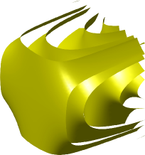
(a) unconnected

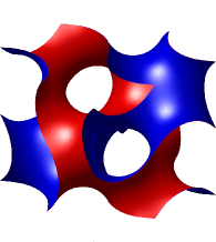
(b) orientable

(c) closed

Figure 1: Examples for iso-surfaces: (a) shows unconnected isosurfaces in $[-1,1]^{3},$ (b) shows that isosurfaces are orientable, (c) shows a closed isosurface.

There is no concept of a boundary when only one level-set function $\phi\left(\mathchoice{\displaystyle\boldsymbol{x}}{\textstyle\boldsymbol{x}}{\scriptstyle\boldsymbol{x}}{\scriptscriptstyle\boldsymbol{x}}\right)$ is considered with $\mathchoice{\displaystyle\boldsymbol{x}}{\textstyle\boldsymbol{x}}{\scriptstyle\boldsymbol{x}}{\scriptscriptstyle\boldsymbol{x}}\in\mathbb{R}^{3}$. As a consequence, isosurfaces with finite area must be closed (compact) as e.g. shown in Fig. 1(c), hence, there is no boundary. Otherwise, in the more general case, they are open and feature an infinite area without a boundary. It is thus seen that the manifold of interest, i.e. the surface $\Gamma$ where a BVP is to be solved, is typically only a subset of $\Gamma_{\phi}$, hence, $\Gamma\subseteq\Gamma_{\phi}$.

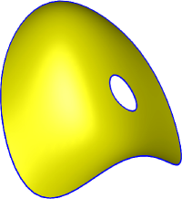
(a) bounded manifold

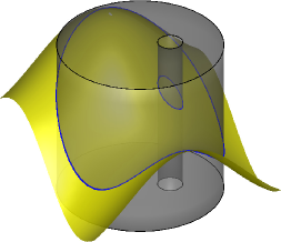
(b) subregion $\Omega$

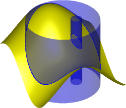
(c) several level-sets

Figure 2: The bounded isosurface in (a) may be described by restricting the evaluation of $\phi\left(\mathchoice{\displaystyle\boldsymbol{x}}{\textstyle\boldsymbol{x}}{\scriptstyle\boldsymbol{x}}{\scriptscriptstyle\boldsymbol{x}}\right)$ to the subregion $\Omega$ shown in (b) or by using additional level-set functions whose isosurfaces are seen in (c).

There are two alternatives to define bounded isosurfaces with finite area, see Fig. 2(a), which fully represent the manifold of interest: One is to evaluate the level-set function $\phi$ only in a subregion $\Omega\in\mathbb{R}^{3}$, hence

$$\Gamma=\left\{\mathchoice{\displaystyle\boldsymbol{x}}{\textstyle\boldsymbol{x}}{\scriptstyle\boldsymbol{x}}{\scriptscriptstyle\boldsymbol{x}}\in\Omega:\,\phi\left(\mathchoice{\displaystyle\boldsymbol{x}}{\textstyle\boldsymbol{x}}{\scriptstyle\boldsymbol{x}}{\scriptscriptstyle\boldsymbol{x}}\right)=0\right\}.$$ (2.2)

See Fig. 2(b) for an example, where $\phi\left(\mathchoice{\displaystyle\boldsymbol{x}}{\textstyle\boldsymbol{x}}{\scriptstyle\boldsymbol{x}}{\scriptscriptstyle\boldsymbol{x}}\right)$ is only evaluated in the gray subregion $\Omega$ instead of $\mathbb{R}^{3}$. The other is to employ additional level-set functions $\psi^{i}\left(\mathchoice{\displaystyle\boldsymbol{x}}{\textstyle\boldsymbol{x}}{\scriptstyle\boldsymbol{x}}{\scriptscriptstyle\boldsymbol{x}}\right)$ to restrict $\Gamma_{\phi}$, hence

$$\Gamma=\left\{\mathchoice{\displaystyle\boldsymbol{x}}{\textstyle\boldsymbol{x}}{\scriptstyle\boldsymbol{x}}{\scriptscriptstyle\boldsymbol{x}}\in\mathbb{R}^{3}:\,\phi\left(\mathchoice{\displaystyle\boldsymbol{x}}{\textstyle\boldsymbol{x}}{\scriptstyle\boldsymbol{x}}{\scriptscriptstyle\boldsymbol{x}}\right)=0\;\mathrm{and}\;\psi^{i}\left(\mathchoice{\displaystyle\boldsymbol{x}}{\textstyle\boldsymbol{x}}{\scriptstyle\boldsymbol{x}}{\scriptscriptstyle\boldsymbol{x}}\right)\leq 0,\,i=1,2...\right\}.$$ (2.3)

See Fig. 2(c) for an example, where two additonal isosurfaces of $\psi^{1}$ and $\psi^{2}$ are shown in blue. The same bounded isosurface from Fig. 2(a) is thereby defined.

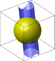
(a) ex. 1, isosurfaces

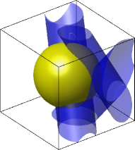
(b) ex. 2, isosurfaces

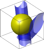
(c) ex. 3, isosurfaces

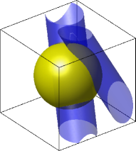
(d) ex. 4, isosurfaces

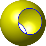
(e) ex. 1, manifold

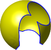
(f) ex. 2, manifold

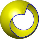
(g) ex. 3, manifold

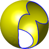
(h) ex. 4, manifold

Figure 3: (a) to (d) show some isosurfaces, yellow of $\phi$ and blue of $\psi^{i}$, (e) to (h) show the implied bounded manifolds (from different viewpoints), respectively. Several continuous $\psi^{i}$ are able to define corners in the boundaries of the manifold.

Further examples are shown in Fig. 3. In Fig. 3(a) to (d), zero-isosurfaces are shown, in yellow of $\phi\left(\mathchoice{\displaystyle\boldsymbol{x}}{\textstyle\boldsymbol{x}}{\scriptstyle\boldsymbol{x}}{\scriptscriptstyle\boldsymbol{x}}\right)$ and in blue of $\psi^{i}\left(\mathchoice{\displaystyle\boldsymbol{x}}{\textstyle\boldsymbol{x}}{\scriptstyle\boldsymbol{x}}{\scriptscriptstyle\boldsymbol{x}}\right)$. It is seen that complex, bounded manifolds are thereby implied, see Fig. 3(e) to (h). It is clear, that it would be very difficult to define such complex manifolds by using only $\phi\left(\mathchoice{\displaystyle\boldsymbol{x}}{\textstyle\boldsymbol{x}}{\scriptstyle\boldsymbol{x}}{\scriptscriptstyle\boldsymbol{x}}\right)$ and defining subregions $\Omega$. Therefore, we prefer the second alternative of using multiple level-set functions which are evaluated in $\mathbb{R}^{3}$. Of course, a combination of these two alternatives is straightforward: This is in particular useful when the outer boundary of the manifold is straight and follows from a box-like subdomain, e.g. $\Omega=[-1,1]^{3}$, but features internal boundaries which are rather described by $\psi^{i}$.

An important consequence of using several level-set functions $\psi^{i}\left(\mathchoice{\displaystyle\boldsymbol{x}}{\textstyle\boldsymbol{x}}{\scriptstyle\boldsymbol{x}}{\scriptscriptstyle\boldsymbol{x}}\right)$ to restrict $\Gamma_{\phi}$ is that corners in the boundaries of the manifold may be defined straightforwardly (although each $\psi^{i}$ is smooth). This seen in Fig. 3(f) to (h) where more than one $\psi^{i}$ is present. It is noted that the employed level-set functions $\phi$ and $\psi^{i}$ do not have to be signed distance functions.

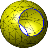
(a) ex. 1, mesh

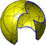
(b) ex. 2, mesh

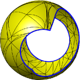
(c) ex. 3, mesh

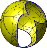
(d) ex. 4, mesh

Figure 4: Some automatically generated higher-order meshes of the bounded manifolds shown in Fig. 3.

The task is now to automatically generate higher-order meshes of the bounded manifolds. See Fig. 4 for some examples of meshes referring to the bounded isosurfaces shown in Fig. 3.

3 Mesh generation of the manifold

The procedure is outlined as follows: First, a background mesh is introduced such that the manifold of interest is completely immersed. The level-set data is evaluated at the nodes of the higher-order elements of this background mesh. Second, the isosurface $\Gamma_{\phi}$ is identified and meshed which is called reconstruction. As mentioned before, this isosurface is either closed or is bounded by the boundary of the background mesh. Third, the meshed isosurface $\Gamma_{\phi}$ is restricted by the additonal level-set functions $\psi^{i}$.

3.1 Background mesh

A background mesh is introduced such that the manifold of interest is completely immersed. The mesh is composed by higher-order background elements of the Lagrange class and we restrict ourselves to tetrahedral elements for simplicity. Hexahedral elements could be decomposed into tetrahedra and treated similarly, see [23]. There are no restrictions on the background mesh, i.e. it may be unstructured and the element faces may be curved.

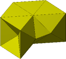
(a) building block

(b) universal mesh

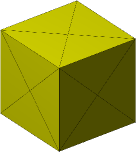
(c) building block

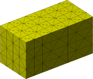
(d) box mesh

Figure 5: Different types of typical background meshes. (a) shows the building block of the universal mesh in (b), (c) shows the building block of the “box mesh” in (d).

We shall later discuss the issue of manipulating the background mesh by moving nodes in order to improve the resulting surface elements of the manifold mesh. We find that the concept of universal meshes [36], extended to three dimensions as shown in Fig. 5(b), allows for a maximum of flexibility in the node movements. But natural choices are also the block-type meshes shown in Fig. 5(d). This is in particular useful when the manifold of interest features straight edges and follows from Eq. (2.2) with a block-type subdomain, e.g. $\Omega=[-1,1]^{3}$.

3.2 Reconstruction of $\Gamma_{\phi}$

In each element of the background mesh which is cut by the zero-isosurface of $\phi$, the task is to identify element nodes of a higher-order surface element on the isosurface. This has been described in detail in the first part of this series of publications, see [24] and also [23]. The procedure is shortly summarized as: In each tetrahedral background element, it is confirmed that valid level-set data is present which implies only two possible cut scenarios of the isosurface: The isosurface is either of triangular shape, see Fig. 6(a), then three edges are cut. Otherwise, four edges are cut and it is of quadrilateral shape, see Fig. 6(b). Depending on the topology, customized search algorithms are evaluated in the reference background element.

First, element nodes on the faces of the tetrahedron are identified leading to the edge nodes of the sought surface element approximating the isosurface. This is, in fact, realized by reconstructing a higher-order line element in a two-dimensional, triangular reference element with the level-set data from the respective face nodes of the tetrahedron. This line is mapped to the corresponding face of the tetrahedron. The inner nodes of the sought surface element are then determined in the reference tetrahedron wherefore the search algorithm also makes use of the position of the edge nodes determined beforehand. Finally, the determined surface element may be mapped to the physical background element using the isoparametric concept. An example is seen in Fig. 6(c) and (d) for the two different topological cases of a triangular or quadrilateral surface element, respectively.

(a) top. 1, ref. element

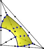
(b) top. 2, ref. element

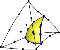
(c) top. 1, real element

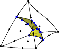
(d) top. 2, real element

Figure 6: (a) and (b) show a triangular or quadrilateral isosurface in the reference background element, respectively, which is approximated by a surface element, (c) and (d) show the mapped situation in a physical element of the background mesh.

Obviously, applying the described procedure in all cut background elements leads to a set of higher-order surface elements representing an accurate approximation of $\Gamma_{\phi}$. Lateron, a mesh suitable for a finite element analysis of the BVP on the manifold will be automatically generated from this element set, see Section 3.4. An important property of such a mesh is that it is at least $C_{0}$-continuous so that there are no gaps in the representation of the manifold. It is interesting to note that the reconstruction described above does, in fact, not assure this property without further considerations.

(a) reference element

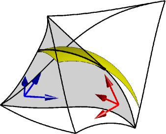
(b) two real elements

Figure 7: (a) shows the convention for the face coordinate systems, normal vectors (red) point outwards, (b) shows two physical elements where the node numberings imply non-matching coordinate systems on the shared face. This will lead to slightly different nodes on the shared edge and, hence, to a small gap in the (yellow) surface elements. Therefore, for the reconstruction on the faces, a permutation may be required to ensure that the face coordinate systems match.

The reason for this is found in the orientation of the face coordinate systems, see Fig. 7: Only when the same coordinate system is used for both tetrahedra sharing a face, this will lead to exactly the same edge nodes of the surface elements. Otherwise, only the corner nodes of the surface elements perfectly match. Fortunately, there is a simple solution to the problem: The face nodes of a tetrahedron which are extracted for the reconstruction of the edge nodes of the sought surface element should be permuted such that they imply the same coordinate systems on the shared face. The resulting set of surface elements is then, as desired, a globally $C_{0}$-continuous, higher-order approximation of $\Gamma_{\phi}$. This is an important difference to the reconstructions discussed in [23, 24].

3.3 Restriction of $\Gamma_{\phi}$ by additional level-set functions $\psi^{i}$

The focus is on one background element cut by the zero-level set of $\phi\left(\mathchoice{\displaystyle\boldsymbol{x}}{\textstyle\boldsymbol{x}}{\scriptstyle\boldsymbol{x}}{\scriptscriptstyle\boldsymbol{x}}\right)$. A triangular or quadrilateral surface element, approximating the zero isosurface, has been succesfully reconstructed. Assume that the background element and the surface element are also cut by another level set function $\psi^{k}\left(\mathchoice{\displaystyle\boldsymbol{x}}{\textstyle\boldsymbol{x}}{\scriptstyle\boldsymbol{x}}{\scriptscriptstyle\boldsymbol{x}}\right)$, see Fig. 8(a) to (c) for different examples. A decomposition of the surface element is then sought into surface elements on the two sides, see Fig. 8(d) to (f) for the same examples, respectively.

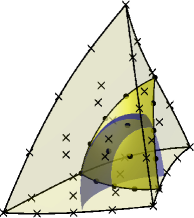
(a) ex. 1, reconstruction

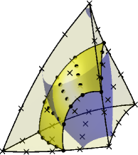
(b) ex. 2, reconstruction

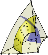
(c) ex. 3, reconstruction

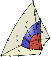
(d) ex. 1, decomposition

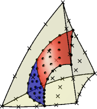
(e) ex. 2, decomposition

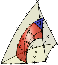
(f) ex. 3, decomposition

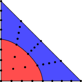
(g) ex. 1, 2D ref. element

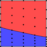
(h) ex. 2, 2D ref. element

(i) ex. 3, 2D ref. element

Figure 8: Example 1 features a triangular surface element, examples 2 and 3 a quadrilateral surface element, (a) to (c) show the reconstructed surface element (yellow) and the zero isosurface of $\psi^{k}$ (blue) cutting through the elements, (d) to (f) show the decomposed surface elements with respect to $\psi^{k}$ (red for $\psi^{k}<0$, blue for $\psi^{k}>0$), (g) to (i) show that the decomposition is realized in 2D reference elements.

For this decomposition, it is necessary to first interpolate the nodal values of $\psi^{k}\left(\mathchoice{\displaystyle\boldsymbol{x}}{\textstyle\boldsymbol{x}}{\scriptstyle\boldsymbol{x}}{\scriptscriptstyle\boldsymbol{x}}\right)$ in the background element (crosses) at the nodes of the reconstructed surface element (dots). Then, the decomposition is carried out in two-dimensional reference elements with these nodal values, see Fig. 8(g) to (i). As discussed in detail in [23, 24], different cut scenarios may be faced: In triangles, always one of the corners is on the other side than the other two and one sub-triangle and one sub-quadrilateral are obtained, see Fig. 8(g). In quadrilaterals, either two neighboring nodes are on the other side leading to two sub-quadrilaterals, see Fig. 8(h), or only one node, leading to four triangles, see Fig. 8(i). The decomposed two-dimensional elements are mapped to the cut tetrahedral element using an isoparametric map implied by the original surface element (from the reconstruction of $\phi$). Typically, considering Eq. (2.3), only the subelements on the negative side of $\psi^{k}$ are needed and the others are neglected, this may be called restriction.

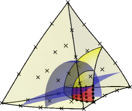
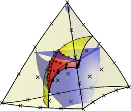
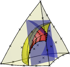
Figure 9: Some examples for level-set functions $\psi^{k}$ further restricting the reconstructed surface element, the corresponding isosurfaces are shown in blue. The final resulting reconstructed elements which approximate $\Gamma_{\phi}$ with $\psi^{k}<0$ are shown in red.

The procedure is very similar when several level-set functions $\psi^{i}\left(\mathchoice{\displaystyle\boldsymbol{x}}{\textstyle\boldsymbol{x}}{\scriptstyle\boldsymbol{x}}{\scriptscriptstyle\boldsymbol{x}}\right)$ cut the same element, possibly implying one or more corners in the boundary of the manifold. The starting point is then a set of surface elements resulting from a previous restriction with respect to other level-set functions. Then, at each surface element, the procedure from above is repeated: The nodal values of the current level-set function at the current surface element are interpolated from the tetrahedral nodes. Then, the decomposition is carried out in the two-dimensional reference elements and mapped to the current surface element. Finally, the resulting sub-elements are restricted to those with $\psi^{i}\left(\mathchoice{\displaystyle\boldsymbol{x}}{\textstyle\boldsymbol{x}}{\scriptstyle\boldsymbol{x}}{\scriptscriptstyle\boldsymbol{x}}\right)<0$. See Fig. 9 for some examples. It is emphasized that the reconstructions are always realized in reference elements (before mapping them to the situation in global coordinates): For the level-set function $\phi$, these are 3D reference tetrahedra and for the level-set functions $\psi^{i}$, these are reference triangular or quadrilateral elements. This enables a very efficient and robust implementation as the reference elements always feature straight edges and planar faces, respectively. On the contrary, it seems impossible to reconstruct directly in general, possibly curved, physical elements.

3.4 Mesh generation

Starting point is a set of higher-order surface elements which has been reconstructed from $\Gamma_{\phi}$ and restricted to the manifold of interest $\Gamma$ using the additional level-set functions $\psi^{k}$. In order to approximate a BVP on the manifold, a finite element mesh has to be generated from the element set. The aim is to extract a set of unique nodes, introduce a global node numbering and set up a connectivity matrix defining the elements. It is noted that the generated element set from above contains triangular and quadrilateral elements, which leads to a mixed finite element mesh. Of course, the decompositon of quadrilateral elements to triangular elements (or vice versa) is possible if meshes of one element type are preferred.

There are two obvious alternatives for the automatic mesh generation from the element set: In alternative 1, the nodes are first sorted with respect to their coordinates and then repeated nodes, such as they appear on the element edges and corners, are unified and associated with a node number. This may be implemented very efficiently, however, it requires some user-defined threshold characterizing a distance within which nodes are considered equal. Because the overall set of elements may contain extremely small elements (e.g. when the zero-isosurface cuts very close to a corner node of a background element) this may interfere with the threshold leading to invalid data. For example, all element nodes may be unified to one node in an extreme situation.

Therefore, we prefer alternative 2 where the connectivity information of the background mesh is employed. One may easily determine the neigboring elements of each tetrahedron. For the surface elements in the reconstructed set of elements, the information of the corresponding background elements is stored, respectively. One may then directly compute which nodes on a shared face of two tetrahedra must match. The same holds for the nodes on a shared edge of several tetrahedra. No distance computations are needed in this approach. It is clear that an advanced implementation is possible where the computation of nodes with the same coordinates (at the edges or corners of the surface elements belonging to different background elements) is completely avoided.

3.5 Manipulation of the background mesh

Some example meshes for complex manifolds are seen in Fig. 4. It is obvious that awkward element shapes result from the automatic meshing. Very small inner angles may occur and the size of neighboring elements can vary strongly so that the shape regularity is an issue. This may lead to the assumption that the elements are not suitable for the analysis, even less in a higher-order context. However, as shown in [31, 33] in a low-order context, only a few manipulations ensure that the “maximal angle condition” is fulfilled and the spectral condition number is bounded uniformly. More generally, it has recently been shown in several publications by the groups around Hansbo, Burman and Reusken, e.g. [5, 33, 38], that optimal results for BVPs on implicitly defined manifolds are possible with such meshes. They use finite element shape functions based on the background mesh which are only evaluated on the manifold; these approaches are labelled TraceFEM or CutFEM. They introduce tailored stabilization terms which avoid negative effects resulting from the ill-shaped elements. We shall report on the use of such methods in this context in a future publication. Herein, we wish to avoid the detailed (mathematical) discussion of these approaches.

A simple and intuitive attempt is to manipulate the background mesh such that the resulting reconstructed elements remain shape regular. In particular, the area of the surface elements shall be bounded from below. When the condition numbers in a finite element analysis obtained by a tailored, manufactured surface mesh, ideally featuring the same element shapes and areas in the whole mesh, are compared to those of the automatically generated meshes from above, it is seen that there is typically an increase by the factor of the largest to the smallest element area $A_{\mathrm{max}}/A_{\mathrm{min}}$. Because $A_{\mathrm{max}}$ typically scales with the size of the (very regular) background elements, this clearly motivates the need to bound $A_{\mathrm{min}}$ from below.

For simplicity, we focus on the set of elements resulting from a reconstruction with respect to $\phi$, i.e. the set of elements approximating $\Gamma_{\phi}$ on a finite background mesh. An algorithm is proposed which moves the nodes of the background mesh away from the zero-level set of $\phi$. Basically, this ensures that the zero-isosurface is not too close to the corner nodes of the background mesh and, consequently, that the surface elements are not too small. Only the nodes in a close band around the zero isosurface are moved.

Although the elements of the background mesh may be arbitrarily curved, it is quite useful to enforce straight edges for simplicity of the node manipulation. The algorithm for the node movement is described for one concrete node at position $\mathchoice{\displaystyle\boldsymbol{x}}{\textstyle\boldsymbol{x}}{\scriptstyle\boldsymbol{x}}{\scriptscriptstyle\boldsymbol{x}}^{{}^{\prime}}$ in the background mesh; the same holds for all other nodes. It may be seen as a fix-point iteration and the following steps are repeated until all nodes have been moved sufficiently away from the zero-level set.

1. Approximate the distance of the node at $\mathchoice{\displaystyle\boldsymbol{x}}{\textstyle\boldsymbol{x}}{\scriptstyle\boldsymbol{x}}{\scriptscriptstyle\boldsymbol{x}}^{\prime}$ to the zero-level set. When the level-set function $\phi$ is given in analytical form, this is realized by a Newton-Raphson procedure,

   $$\mathchoice{\displaystyle\boldsymbol{x}}{\textstyle\boldsymbol{x}}{\scriptstyle\boldsymbol{x}}{\scriptscriptstyle\boldsymbol{x}}_{i+1}=\mathchoice{\displaystyle\boldsymbol{x}}{\textstyle\boldsymbol{x}}{\scriptstyle\boldsymbol{x}}{\scriptscriptstyle\boldsymbol{x}}_{i}-\frac{\phi\left(\mathchoice{\displaystyle\boldsymbol{x}}{\textstyle\boldsymbol{x}}{\scriptstyle\boldsymbol{x}}{\scriptscriptstyle\boldsymbol{x}}_{i}\right)}{\left\|\nabla\phi\left(\mathchoice{\displaystyle\boldsymbol{x}}{\textstyle\boldsymbol{x}}{\scriptstyle\boldsymbol{x}}{\scriptscriptstyle\boldsymbol{x}}_{i}\right)\right\|}\cdot\nabla\phi\left(\mathchoice{\displaystyle\boldsymbol{x}}{\textstyle\boldsymbol{x}}{\scriptstyle\boldsymbol{x}}{\scriptscriptstyle\boldsymbol{x}}_{i}\right),$$

   using $\mathchoice{\displaystyle\boldsymbol{x}}{\textstyle\boldsymbol{x}}{\scriptstyle\boldsymbol{x}}{\scriptscriptstyle\boldsymbol{x}}_{0}=\mathchoice{\displaystyle\boldsymbol{x}}{\textstyle\boldsymbol{x}}{\scriptstyle\boldsymbol{x}}{\scriptscriptstyle\boldsymbol{x}}^{\prime}$ as the starting point. This algorithm converges to some position $\mathchoice{\displaystyle\boldsymbol{x}}{\textstyle\boldsymbol{x}}{\scriptstyle\boldsymbol{x}}{\scriptscriptstyle\boldsymbol{x}}^{\star}$ on the zero-level set which is not necessarily the closest point. However, it is found that $\mathchoice{\displaystyle\boldsymbol{x}}{\textstyle\boldsymbol{x}}{\scriptstyle\boldsymbol{x}}{\scriptscriptstyle\boldsymbol{x}}^{\star}$ is approaching the closest point quickly the closer $\mathchoice{\displaystyle\boldsymbol{x}}{\textstyle\boldsymbol{x}}{\scriptstyle\boldsymbol{x}}{\scriptscriptstyle\boldsymbol{x}}^{{}^{\prime}}$ is to the zero-level set. Because the node manipulation is only realized for nodes which are close to the zero-level set, it turned out to be sufficient to continue with the computed position $\mathchoice{\displaystyle\boldsymbol{x}}{\textstyle\boldsymbol{x}}{\scriptstyle\boldsymbol{x}}{\scriptscriptstyle\boldsymbol{x}}^{\star}$. The estimated signed distance is

   $$D\left(\mathchoice{\displaystyle\boldsymbol{x}}{\textstyle\boldsymbol{x}}{\scriptstyle\boldsymbol{x}}{\scriptscriptstyle\boldsymbol{x}}^{\prime}\right)=\left\|\mathchoice{\displaystyle\boldsymbol{x}}{\textstyle\boldsymbol{x}}{\scriptstyle\boldsymbol{x}}{\scriptscriptstyle\boldsymbol{x}}^{\prime}-\mathchoice{\displaystyle\boldsymbol{x}}{\textstyle\boldsymbol{x}}{\scriptstyle\boldsymbol{x}}{\scriptscriptstyle\boldsymbol{x}}^{\star}\right\|\cdot\mathrm{sign}\left(\phi\left(\mathchoice{\displaystyle\boldsymbol{x}}{\textstyle\boldsymbol{x}}{\scriptstyle\boldsymbol{x}}{\scriptscriptstyle\boldsymbol{x}}^{\prime}\right)\right)$$

   and the direction

   $$\mathchoice{\displaystyle\boldsymbol{d}}{\textstyle\boldsymbol{d}}{\scriptstyle\boldsymbol{d}}{\scriptscriptstyle\boldsymbol{d}}\left(\mathchoice{\displaystyle\boldsymbol{x}}{\textstyle\boldsymbol{x}}{\scriptstyle\boldsymbol{x}}{\scriptscriptstyle\boldsymbol{x}}^{\prime}\right)=\frac{\left(\mathchoice{\displaystyle\boldsymbol{x}}{\textstyle\boldsymbol{x}}{\scriptstyle\boldsymbol{x}}{\scriptscriptstyle\boldsymbol{x}}^{\prime}-\mathchoice{\displaystyle\boldsymbol{x}}{\textstyle\boldsymbol{x}}{\scriptstyle\boldsymbol{x}}{\scriptscriptstyle\boldsymbol{x}}^{\star}\right)}{D\left(\mathchoice{\displaystyle\boldsymbol{x}}{\textstyle\boldsymbol{x}}{\scriptstyle\boldsymbol{x}}{\scriptscriptstyle\boldsymbol{x}}^{{}^{\prime}}\right)}$$

   is computed as well; there holds $\left\|\mathchoice{\displaystyle\boldsymbol{d}}{\textstyle\boldsymbol{d}}{\scriptstyle\boldsymbol{d}}{\scriptscriptstyle\boldsymbol{d}}\left(\mathchoice{\displaystyle\boldsymbol{x}}{\textstyle\boldsymbol{x}}{\scriptstyle\boldsymbol{x}}{\scriptscriptstyle\boldsymbol{x}}^{\prime}\right)\right\|=1$. In the case that $\phi$ is only given at the nodes of a higher-order background mesh (and no analytic information is available), one may estimate the distance through a linear reconstruction of the zero isosurface which is much cheaper than the desired higher-order reconstruction performed after the node manipulation.

2. Move the node provided that it is sufficiently close to the zero-level set, i.e. when $\left|D\left(\mathchoice{\displaystyle\boldsymbol{x}}{\textstyle\boldsymbol{x}}{\scriptstyle\boldsymbol{x}}{\scriptscriptstyle\boldsymbol{x}}^{\prime}\right)\right|<D_{\mathrm{crit}}$. $D_{\mathrm{crit}}$ scales with the resolution of the background mesh and we typically set $D_{\mathrm{crit}}=3\cdot h$ with $h$ being some characteristic element length. The node is moved as

   $$\mathchoice{\displaystyle\boldsymbol{x}}{\textstyle\boldsymbol{x}}{\scriptstyle\boldsymbol{x}}{\scriptscriptstyle\boldsymbol{x}}^{\prime\prime}=\mathchoice{\displaystyle\boldsymbol{x}}{\textstyle\boldsymbol{x}}{\scriptstyle\boldsymbol{x}}{\scriptscriptstyle\boldsymbol{x}}^{\prime}+q\left(D,D_{\mathrm{crit}},D_{\mathrm{step}}\right)\cdot\mathchoice{\displaystyle\boldsymbol{d}}{\textstyle\boldsymbol{d}}{\scriptstyle\boldsymbol{d}}{\scriptscriptstyle\boldsymbol{d}}\left(\mathchoice{\displaystyle\boldsymbol{x}}{\textstyle\boldsymbol{x}}{\scriptstyle\boldsymbol{x}}{\scriptscriptstyle\boldsymbol{x}}^{\prime}\right)\cdot\mathrm{sign}\left(D\left(\mathchoice{\displaystyle\boldsymbol{x}}{\textstyle\boldsymbol{x}}{\scriptstyle\boldsymbol{x}}{\scriptscriptstyle\boldsymbol{x}}^{\prime}\right)\right)$$

   with

   $$q\left(D,D_{\mathrm{crit}},D_{\mathrm{step}}\right)=D_{\mathrm{step}}\cdot\left(1-\frac{\left|D\right|}{D_{\mathrm{crit}}}\right).$$

   That is, the maximum distance a node is moved in one step is $D_{\mathrm{step}}$ which is often set as $0.1\cdot h$. Obviously, $q$ scales linearly with the distance of a node from the zero-level set.

3. Set $\mathchoice{\displaystyle\boldsymbol{x}}{\textstyle\boldsymbol{x}}{\scriptstyle\boldsymbol{x}}{\scriptscriptstyle\boldsymbol{x}}^{\prime}=\mathchoice{\displaystyle\boldsymbol{x}}{\textstyle\boldsymbol{x}}{\scriptstyle\boldsymbol{x}}{\scriptscriptstyle\boldsymbol{x}}^{\prime\prime}$ and repeat the two steps from above until $\left|D\left(\mathchoice{\displaystyle\boldsymbol{x}}{\textstyle\boldsymbol{x}}{\scriptstyle\boldsymbol{x}}{\scriptscriptstyle\boldsymbol{x}}^{\prime}\right)\right|>D_{\mathrm{min}}$ where, typically, $D_{\mathrm{min}}=0.25\cdot h$.

This algorithm works very fast and scales linearly with the number of nodes in the background mesh. It is controlled by the three parameters which are summarized as: $D_{\mathrm{crit}}$ and $D_{\mathrm{min}}$ define local regions around the zero-level sets (“bands”): Nodes within the band controlled by $D_{\mathrm{crit}}$ are considered for movement and $D_{\mathrm{min}}$ defines the band within which no nodes shall be present. $D_{\mathrm{step}}$ defines the maximum moving length in one iteration which is scaled linearly in the band controlled by $D_{\mathrm{crit}}$. Obviously, we need $D_{\mathrm{step}}<D_{\mathrm{min}}<D_{\mathrm{crit}}$.

It is mentioned that in our first approximations of BVPs on manifolds with the automatically generated surface meshes, we were surprised by the accuracy of the results even without any mesh manipulations. Actually, it seems that as long as direct solvers are employed (in our case Matlab’s backslash solver), there is a large range of condition numbers still leading to accurate results even in the frame of systematic convergence studies. Nevertheless, the node manipulations are used by default in the numerical studies presented in Section 5. It is an important advantage that they also render recursive refinements of the background elements unnecessary as long as the resolution of the background elements is reasonably adjusted to the complexity of the zero-level sets. The effect of the proposed node manipulation is now demonstrated in one, two an three dimensions.

3.5.1 Node manipulation in 1D

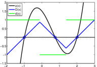
(a) $\phi,D,d$

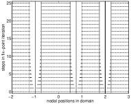
(b) Example 1

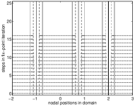
(c) Example 2

(d) Example 3

Figure 10: Examples for node movements in 1D, (a) shows a level-set function $\phi$ (black), the corresponding signed-distance function $D$ (blue) and its gradient $d$ (green), (b) to (d) show how the nodes within $D_{\mathrm{crit}}$ are moved away from the roots during the fix-point iteration.

Consider the one-dimensional example shown in Fig. 10. In Fig. 10(a), a level-set function $\phi$ is plotted in black and the corresponding signed-distance function $D$, which stores the (signed) distance to the closest root of $\phi$, is shown in blue. On the $x$-axis, there are regularly distributed nodes marked as blacked dots, the distance between two nodes is $h$. The aim is to move these nodes away from the roots (blue circles). In Fig. 10(b), we set $D_{\mathrm{crit}}=D_{\mathrm{min}}=5\cdot h$ and $D_{\mathrm{step}}=h$. It is then seen that after about 10 steps of the fix-point iteration, the nodes in the region $D_{\mathrm{crit}}$ are squeezed to the boundary between the band scaled by $D_{\mathrm{crit}}$ and the rest of the domain. The resulting nodal distribution leads to undesired, locally concentrated background elements. Therefore, we set $D_{\mathrm{crit}}=5\cdot h$ and $D_{\mathrm{min}}=\nicefrac{{1}}{{2}}D_{\mathrm{crit}}$ next. Results with $D_{\mathrm{step}}=\nicefrac{{1}}{{5}}h$ and $\nicefrac{{1}}{{2}}h$ are shown in Figs. 10(c) and (d), respectively. Obviously, the larger the value for $D_{\mathrm{step}}$, the faster the nodes are moved out of the band controlled by $D_{\mathrm{min}}$. Nevertheless, in more than one dimension, setting $D_{\mathrm{step}}$ considerably smaller than $D_{\mathrm{min}}$ allows for curved node paths throughout the nodal movements leading to smoother element distributions in the background meshes.

3.5.2 Node manipulation in 2D and 3D

(a) $\phi_{1}$, coarse

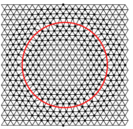
(b) $\phi_{1}$, fine

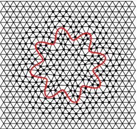
(c) $\phi_{2}$, coarse

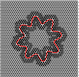
(d) $\phi_{2}$, fine

Figure 11: Examples for node movements in 2D based on different level-set functions $\phi$ and background meshes. The red lines are the zero isolines $\Gamma_{\phi_{i}}$ which are meshed by higher-order line elements.

Examples for manipulations of background meshes in 2D are shown in Fig. 11. Two different level-set functions $\phi$ on a coarse and a fine mesh are considered, respectively. The red lines indicate the zero-level sets which are meshed by higher-order line elements. It is seen that due to the nodal movements, the lengths of the line elements in the background mesh are quite regular, hence, the ratio $l_{\mathrm{max}}/l_{\mathrm{min}}$ is bounded. The results are achieved with $D_{\mathrm{crit}}=3\cdot h$, $D_{\mathrm{min}}=0.25\cdot h$, and $D_{\mathrm{step}}=0.1\cdot h$.

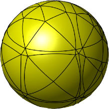
(a) $\Gamma_{\phi_{1}}$, coarse

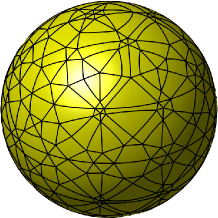
(b) $\Gamma_{\phi_{1}}$, medium

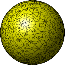
(c) $\Gamma_{\phi_{1}}$, fine

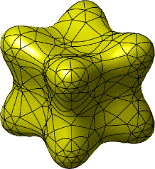
(d) $\Gamma_{\phi_{2}}$, coarse

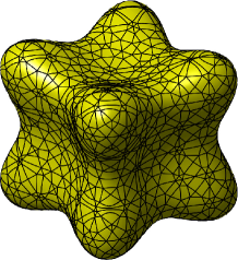
(e) $\Gamma_{\phi_{2}}$, medium

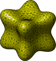
(f) $\Gamma_{\phi_{2}}$, fine

Figure 12: Examples for node movements in 3D based on different level-set functions $\phi$ and background meshes (not shown).

A similar study is repeated in 3D. In Fig. 12, the resulting surface meshes are shown for two different level-set functions on different background meshes, respectively. The manipulated background meshes are omitted for clarity and the focus is on the shape and size of the surface elements. The element areas of the largest and smallest elements are computed and given in Tables 1 and 2. As can be seen, the ratio $A_{\mathrm{max}}/A_{\mathrm{min}}$ is well bounded; it is typically less than $100$. The increase in the condition number when using the automatically generated meshes as proposed herein (compared to manually constructed meshes) is in the same range. This is not a problem as long as direct solvers are employed, however, will increase the effort in the context of iterative solvers.

$\phi_{1}$	$A_{\mathrm{max}}$	$A_{\mathrm{min}}$	$A_{\mathrm{max}}/A_{\mathrm{min}}$
coarse mesh	$1.51\cdot 10^{-1}$	$1.63\cdot 10^{-3}$	$93.1$
medium mesh	$3.69\cdot 10^{-2}$	$6.23\cdot 10^{-4}$	$59.2$
fine mesh	$6.72\cdot 10^{-3}$	$1.84\cdot 10^{-4}$	$36.5$

Table 1: Element areas of the surface meshes resulting from $\phi_{1}$ as shown in Fig. 12 (a) to (c).

$\phi_{2}$	$A_{\mathrm{max}}$	$A_{\mathrm{min}}$	$A_{\mathrm{max}}/A_{\mathrm{min}}$
coarse mesh	$3.20\cdot 10^{-2}$	$7.35\cdot 10^{-4}$	$43.6$
medium mesh	$1.07\cdot 10^{-2}$	$1.33\cdot 10^{-4}$	$81.0$
fine mesh	$1.88\cdot 10^{-3}$	$4.31\cdot 10^{-5}$	$43.7$

Table 2: Element areas of the surface meshes resulting from $\phi_{2}$ as shown in Fig. 12 (d) to (f).

4 PDEs on manifolds

Herein, we consider the stationary Poisson equation and the instationary advection-diffusion equation on curved manifolds. Both involve the Laplace-Beltrami operator. The PDEs are conveniently defined based on the tangential differential calculus, i.e. on surface gradients (sometimes refered to as intrinsic gradients). The manifold $\Gamma$ is implicitly defined by the zero-level set of a sufficiently smooth level-set function. The tangential gradient operator $\nabla_{\Gamma}$ of a scalar function $u:\Gamma\to\mathbb{R}$ on the manifold is defined as

$$\nabla_{\Gamma}u=\mathchoice{\displaystyle\mathbf{P}}{\textstyle\mathbf{P}}{\scriptstyle\mathbf{P}}{\scriptscriptstyle\mathbf{P}}\cdot\nabla\tilde{u}=\left(\mathbb{I}-\mathchoice{\displaystyle\boldsymbol{n}}{\textstyle\boldsymbol{n}}{\scriptstyle\boldsymbol{n}}{\scriptscriptstyle\boldsymbol{n}}_{\Gamma}\otimes\mathchoice{\displaystyle\boldsymbol{n}}{\textstyle\boldsymbol{n}}{\scriptstyle\boldsymbol{n}}{\scriptscriptstyle\boldsymbol{n}}_{\Gamma}\right)\cdot\nabla\tilde{u}$$ .

$\mathchoice{\displaystyle\mathbf{P}}{\textstyle\mathbf{P}}{\scriptstyle\mathbf{P}}{\scriptscriptstyle\mathbf{P}}$ is the discrete tangential projector, $\mathchoice{\displaystyle\boldsymbol{n}}{\textstyle\boldsymbol{n}}{\scriptstyle\boldsymbol{n}}{\scriptscriptstyle\boldsymbol{n}}_{\Gamma}$ is the unit normal vektor on the manifold $\Gamma$ and $\tilde{u}$ is a smooth extension in a neighborhood $\mathcal{U}$ of the manifold $\Gamma$. With the tangential divergence of a vector $\mathchoice{\displaystyle\boldsymbol{v}}{\textstyle\boldsymbol{v}}{\scriptstyle\boldsymbol{v}}{\scriptscriptstyle\boldsymbol{v}}$, $\nabla_{\Gamma}\cdot\mathchoice{\displaystyle\boldsymbol{v}}{\textstyle\boldsymbol{v}}{\scriptstyle\boldsymbol{v}}{\scriptscriptstyle\boldsymbol{v}}=\text{tr}(\nabla_{\Gamma}\mathchoice{\displaystyle\boldsymbol{v}}{\textstyle\boldsymbol{v}}{\scriptstyle\boldsymbol{v}}{\scriptscriptstyle\boldsymbol{v}})$, the Laplace-Beltrami operator is [31, 20]

$$\Delta_{\Gamma}u=\nabla_{\Gamma}\cdot\nabla_{\Gamma}u\qquad\text{on}\;\Gamma.$$ (4.1)

Assume a sucessfull reconstruction of the manifold $\Gamma$, the discrete surface $\Gamma_{h}$ is the union of the elements $\Gamma_{h}=\underset{T\in\tau_{h}}{\bigcup}T$, where $\tau_{h}$ is the set of automatically generated Lagrange elements as described above. The standard surface FEM as described in [12, 20] is used to solve the PDEs on the discrete manifold. In the context of the FEM the function $u$ is often a shape function $N\left(\mathchoice{\displaystyle\boldsymbol{r}}{\textstyle\boldsymbol{r}}{\scriptstyle\boldsymbol{r}}{\scriptscriptstyle\boldsymbol{r}}\right)$ living in a reference element $\bar{T}$ with coordinates $\mathchoice{\displaystyle\boldsymbol{r}}{\textstyle\boldsymbol{r}}{\scriptstyle\boldsymbol{r}}{\scriptscriptstyle\boldsymbol{r}}$. Using the standard isoparametric mapping from the reference element to the physical element, $\mathchoice{\displaystyle\boldsymbol{\chi}}{\textstyle\boldsymbol{\chi}}{\scriptstyle\boldsymbol{\chi}}{\scriptscriptstyle\boldsymbol{\chi}}:=\sum_{i}N_{i}\left(\mathchoice{\displaystyle\boldsymbol{r}}{\textstyle\boldsymbol{r}}{\scriptstyle\boldsymbol{r}}{\scriptscriptstyle\boldsymbol{r}}\right)\cdot\mathchoice{\displaystyle\boldsymbol{x}}{\textstyle\boldsymbol{x}}{\scriptstyle\boldsymbol{x}}{\scriptscriptstyle\boldsymbol{x}}_{i},\ \mathchoice{\displaystyle\boldsymbol{r}}{\textstyle\boldsymbol{r}}{\scriptstyle\boldsymbol{r}}{\scriptscriptstyle\boldsymbol{r}}\in\bar{T}$, and $\mathchoice{\displaystyle\boldsymbol{x}}{\textstyle\boldsymbol{x}}{\scriptstyle\boldsymbol{x}}{\scriptscriptstyle\boldsymbol{x}}_{i}\in T$ being nodal coordinates, the finite element space on $\Gamma_{h}$ with the polynomial degree $k$ is then defined by

$$\mathcal{S}_{h}^{k}=\left\{u_{h}\in C\text{\textsuperscript{0}}\left(\Gamma_{h}^{k}\right)\mid u_{h}\circ\mathchoice{\displaystyle\boldsymbol{\chi}}{\textstyle\boldsymbol{\chi}}{\scriptstyle\boldsymbol{\chi}}{\scriptscriptstyle\boldsymbol{\chi}}^{-1}|_{T}\in\mathbb{P}_{k}\left(\bar{T}\right)\;\text{or}\;\mathbb{Q}_{k}\left(\bar{T}\right),T\in\tau_{h}\right\}.$$ (4.2)

$\mathbb{P}_{k}\left(\bar{T}\right)$ is the polynomial basis in a triangular element and $\mathbb{Q}_{k}\left(\bar{T}\right)$ in a quadrilateral element, both being complete of order $k$. This space is spanned by the nodal basis $M_{1},\ldots,\,M_{n}$, with $n$ being the total number of nodes, which is given by

$$M_{i}\left(\mathchoice{\displaystyle\boldsymbol{x}}{\textstyle\boldsymbol{x}}{\scriptstyle\boldsymbol{x}}{\scriptscriptstyle\boldsymbol{x}}\right)\in S_{h}^{k},\qquad M_{i}(\mathchoice{\displaystyle\boldsymbol{x}}{\textstyle\boldsymbol{x}}{\scriptstyle\boldsymbol{x}}{\scriptscriptstyle\boldsymbol{x}}_{j})=\delta_{ij}\ .$$

A base function is defined by $M_{i}=N_{i}\circ\mathchoice{\displaystyle\boldsymbol{\chi}}{\textstyle\boldsymbol{\chi}}{\scriptstyle\boldsymbol{\chi}}{\scriptscriptstyle\boldsymbol{\chi}}|_{T}$. Note that the function space $\mathcal{S}_{h}^{k}$ is a subspace of the continuous space $\mathcal{H}^{1}(\Gamma_{h})$. For more information we refer to [12, 20].

In general, it is desirable to compute the surface gradient without explicitly computing an extension $\tilde{u}$. Assume that the surface element $T$ in the physical space $\mathchoice{\displaystyle\boldsymbol{x}}{\textstyle\boldsymbol{x}}{\scriptstyle\boldsymbol{x}}{\scriptscriptstyle\boldsymbol{x}}\in\mathbb{R}^{3}$ follows from the standard isoparametric mapping $\mathchoice{\displaystyle\boldsymbol{\chi}}{\textstyle\boldsymbol{\chi}}{\scriptstyle\boldsymbol{\chi}}{\scriptscriptstyle\boldsymbol{\chi}}$, then the surface gradient is directly obtained from

$$\nabla_{\Gamma_{h}}u_{h}\left(\mathchoice{\displaystyle\boldsymbol{x}}{\textstyle\boldsymbol{x}}{\scriptstyle\boldsymbol{x}}{\scriptscriptstyle\boldsymbol{x}}\left(\mathchoice{\displaystyle\boldsymbol{r}}{\textstyle\boldsymbol{r}}{\scriptstyle\boldsymbol{r}}{\scriptscriptstyle\boldsymbol{r}}\right)\right)=\mathchoice{\displaystyle\mathbf{J}}{\textstyle\mathbf{J}}{\scriptstyle\mathbf{J}}{\scriptscriptstyle\mathbf{J}}\cdot\mathchoice{\displaystyle\mathbf{G}}{\textstyle\mathbf{G}}{\scriptstyle\mathbf{G}}{\scriptscriptstyle\mathbf{G}}^{-1}\cdot\nabla_{\mathchoice{\displaystyle\boldsymbol{r}}{\textstyle\boldsymbol{r}}{\scriptstyle\boldsymbol{r}}{\scriptscriptstyle\boldsymbol{r}}}u_{h}\left(\mathchoice{\displaystyle\boldsymbol{r}}{\textstyle\boldsymbol{r}}{\scriptstyle\boldsymbol{r}}{\scriptscriptstyle\boldsymbol{r}}\right)$$ (4.3)

with $\mathchoice{\displaystyle\mathbf{J}}{\textstyle\mathbf{J}}{\scriptstyle\mathbf{J}}{\scriptscriptstyle\mathbf{J}}=\nicefrac{{\partial\mathchoice{\displaystyle\boldsymbol{\chi}}{\textstyle\boldsymbol{\chi}}{\scriptstyle\boldsymbol{\chi}}{\scriptscriptstyle\boldsymbol{\chi}}}}{{\partial\mathchoice{\displaystyle\boldsymbol{r}}{\textstyle\boldsymbol{r}}{\scriptstyle\boldsymbol{r}}{\scriptscriptstyle\boldsymbol{r}}}}$ being the ($3\times 2$)-Jacobi matrix and $\mathchoice{\displaystyle\mathbf{G}}{\textstyle\mathbf{G}}{\scriptstyle\mathbf{G}}{\scriptscriptstyle\mathbf{G}}=\mathchoice{\displaystyle\mathbf{J}}{\textstyle\mathbf{J}}{\scriptstyle\mathbf{J}}{\scriptscriptstyle\mathbf{J}}^{T}\cdot\mathchoice{\displaystyle\mathbf{J}}{\textstyle\mathbf{J}}{\scriptstyle\mathbf{J}}{\scriptscriptstyle\mathbf{J}}$ being the first fundamental form.

4.1 Stationary Poisson equation on manifolds

The complete boundary value problem in strong form for the Poisson equation on manifolds states that we seek $u:\Gamma\to\mathbb{R}$ such that:

$$-\Delta_{\Gamma}u =f \text{on}\quad\Gamma,$$ (4.4a)

$$u =g_{\mathrm{D}}\quad \text{on}\quad\partial\Gamma_{\text{D}},$$ (4.4b)

$$\mathchoice{\displaystyle\boldsymbol{n}}{\textstyle\boldsymbol{n}}{\scriptstyle\boldsymbol{n}}{\scriptscriptstyle\boldsymbol{n}}_{\partial\Gamma}\cdot\nabla_{\Gamma}u =g_{\mathrm{N}} \text{on}\quad\partial\Gamma_{\text{N}},$$ (4.4c)

where $f\in L^{2}(\Gamma)$ is a source function and $\mathchoice{\displaystyle\boldsymbol{n}}{\textstyle\boldsymbol{n}}{\scriptstyle\boldsymbol{n}}{\scriptscriptstyle\boldsymbol{n}}_{\partial\Gamma}$ is the co-normal vector being normal to the boundary yet in the tangent plane of the manifold at each point on the boundary.

For a closed (compact) manifold, where no boundary exists, one needs an additional condition for the problem to be well-posed. Therefore, typically the zero mean constraint is imposed,

$$\int\limits_{\Gamma}u\,\text{d}s=0.$$ (4.5)

The boundary value problem from above is converted to a weak form and discretized using the surface FEM. Therefore, we introduce the following trial and test function spaces

$$\mathcal{S}_{u} = \left\{u_{h}\in\mathcal{S}_{h}^{k}(\Gamma_{h})\ :\ u\rvert_{\partial\Gamma_{h,D}}=g_{\mathrm{D}}\right\},$$ (4.6)

$$\mathcal{V}_{u} = \left\{v_{h}\in\mathcal{S}_{h}^{k}(\Gamma_{h})\ :\ v\rvert_{\partial\Gamma_{h,D}}=0\right\}\qquad\mathrm{for\;manifolds\;with\;boundary},$$ (4.7)

$$\mathcal{V}_{u} = \big{\{}v_{h}\in\mathcal{S}_{h}^{k}(\Gamma_{h})\ :\ \smallint_{\Gamma_{h}}v_{h}\,\text{\text{\text{d}}}s=0\big{\}}\qquad\mathrm{for\;compact\;manifolds}.$$ (4.8)

Then, the discrete weak form for the Poisson equation on a manifold $\Gamma_{h}$ is stated as: Find $u_{h}\in\mathcal{S}_{u}$ such that

$$\int\limits_{\Gamma_{h}}\nabla_{\Gamma_{h}}v_{h}\cdot\nabla_{\Gamma_{h}}u_{h}\;\text{\text{d}}s=\int\limits_{\Gamma_{h}}v_{h}\cdot f\;\text{\text{d}}s+\int_{\partial\Gamma_{h}}v_{h}\cdot g_{\mathrm{N}}^{h}\;\text{\text{d}}q\qquad\forall v_{h}\in\mathcal{V}_{u}.$$ (4.9)

The existence and uniqueness of this BVP is shown in [20, 6]. The zero mean constraint for compact manifolds is enforced by a Lagrange multiplier.

4.2 Instationary advection-diffusion equation on manifolds

The strong form of the instationary advection-diffusion equation in the time interval from $0$ to $T$ reads

$$\dot{u}+\mathchoice{\displaystyle\boldsymbol{c}}{\textstyle\boldsymbol{c}}{\scriptstyle\boldsymbol{c}}{\scriptscriptstyle\boldsymbol{c}}_{\Gamma}\cdot\nabla_{\Gamma}u-\lambda\Delta_{\Gamma}u =f \quad\Gamma\times\left(0,T\right),$$ on (4.10a)

$$u =g_{\mathrm{D}} \quad\partial\Gamma_{\text{D}}\times\left(0,T\right),$$ on (4.10b)

$$\mathchoice{\displaystyle\boldsymbol{n}}{\textstyle\boldsymbol{n}}{\scriptstyle\boldsymbol{n}}{\scriptscriptstyle\boldsymbol{n}}_{\partial\Gamma}\cdot\nabla_{\Gamma}u =g_{\mathrm{N}} \quad\partial\Gamma_{\mathrm{N}}\times\left(0,T\right),$$ on (4.10c)

$$u(\mathchoice{\displaystyle\boldsymbol{x}}{\textstyle\boldsymbol{x}}{\scriptstyle\boldsymbol{x}}{\scriptscriptstyle\boldsymbol{x}},0) =u_{0}(\mathchoice{\displaystyle\boldsymbol{x}}{\textstyle\boldsymbol{x}}{\scriptstyle\boldsymbol{x}}{\scriptscriptstyle\boldsymbol{x}})\quad \quad\Gamma\;\mathrm{at}\;t=0,$$ on (4.10d)

with $\dot{u}=\nicefrac{{\partial u}}{{\partial t}}$, $\mathchoice{\displaystyle\boldsymbol{c}}{\textstyle\boldsymbol{c}}{\scriptstyle\boldsymbol{c}}{\scriptscriptstyle\boldsymbol{c}}_{\Gamma}$ being the advection velocity in the tangent space of the manifold and $\lambda$ the diffusion coefficient. Using the same function spaces from above, the semi-discrete weak form becomes: Find $u_{h}\in\mathcal{S}_{u}\times\left(0,T\right)$ with $\dot{u}_{h}\in L^{2}(\Gamma_{h})$ such that $\forall v_{h}\in\mathcal{V}_{u}$

$$\int\limits_{\Gamma_{h}}\left[v_{h}\cdot\dot{u}+v_{h}\cdot\mathchoice{\displaystyle\boldsymbol{c}}{\textstyle\boldsymbol{c}}{\scriptstyle\boldsymbol{c}}{\scriptscriptstyle\boldsymbol{c}}_{\Gamma}\cdot\nabla_{\Gamma_{h}}u_{h}+\lambda\cdot\nabla_{\Gamma_{h}}v_{h}\cdot\nabla_{\Gamma_{h}}u_{h}\right]\text{\text{d}}s=\int\limits_{\Gamma_{h}}v_{h}\cdot f(\mathchoice{\displaystyle\boldsymbol{x}}{\textstyle\boldsymbol{x}}{\scriptstyle\boldsymbol{x}}{\scriptscriptstyle\boldsymbol{x}},t)\;\text{\text{d}}s+\int_{\partial\Gamma_{h}}v_{h}\cdot g_{\mathrm{N}}^{h}\;\text{\text{d}}q.$$ (4.11)

The zero mean constraint from (4.8) for compact manifolds is not needed here. The existence and uniqueness of the solution is guaranteed by the Lax-Milgramm lemma and is proven for the stationary problem in [34].

After the FEM discretization in space, a first-order system of ordinary differential equations in time is obtained as usual. We use a $6$th-order accurate, implicit, $3$-step Runge-Kutta method based on Gauss-Legendre points to discretize in time. The corresponding Butcher tableau for this Runge-Kutta scheme is given as

$$\left[\begin{array}[]{c|c}\mathchoice{\displaystyle\boldsymbol{c}}{\textstyle\boldsymbol{c}}{\scriptstyle\boldsymbol{c}}{\scriptscriptstyle\boldsymbol{c}}&\mathchoice{\displaystyle\mathbf{A}}{\textstyle\mathbf{A}}{\scriptstyle\mathbf{A}}{\scriptscriptstyle\mathbf{A}}\\ \hline\cr&\mathchoice{\displaystyle\boldsymbol{b}}{\textstyle\boldsymbol{b}}{\scriptstyle\boldsymbol{b}}{\scriptscriptstyle\boldsymbol{b}}^{T}\end{array}\right]=\left[\begin{array}[]{c|ccc}\frac{1}{2}-\frac{1}{10}\sqrt{15}&\frac{5}{36}&\frac{2}{9}-\frac{1}{15}\sqrt{15}&\frac{5}{36}-\frac{1}{30}\sqrt{15}\\ \frac{1}{2}&\frac{5}{36}+\frac{1}{24}\sqrt{15}&\frac{2}{9}&\frac{5}{36}-\frac{1}{24}\sqrt{15}\\ \frac{1}{2}+\frac{1}{10}\sqrt{15}&\frac{5}{36}+\frac{1}{30}\sqrt{15}&\frac{2}{9}-\frac{1}{15}\sqrt{15}&\frac{5}{36}\\ \hline\cr&\frac{5}{18}&\frac{4}{9}&\frac{5}{18}\end{array}\right]$$ (4.12)

It is useful to employ this highly accurate scheme in time to virtually eliminate the temporal error in the numerical studies and focus on the spatial approximation error of the surface finite elements (with different orders).

5 Numerical results

As defined in the previous section, the stationary Poisson equation and the instationary advection-diffusion equation are considered here. The focus above is on curved surfaces in three domensions, however, results are also shown for curved lines in two dimensions. Convergence studies for different element orders up to $6$ are conducted where the analytic solutions are generated by the method of manufactured solutions. In each test case, we compare the performance of handcrafted meshes composed by very regular elements with the automatically generated meshes as described in Section 3. The manipulation of the background mesh from Section 3.5 is enabled in all examples.

According to the method of manufactured solutions in the context of the Poisson equation, the source function $f$ on the right hand side is computed such that Eq. (4.4a) is fulfilled for a chosen solution $u(\mathchoice{\displaystyle\boldsymbol{x}}{\textstyle\boldsymbol{x}}{\scriptstyle\boldsymbol{x}}{\scriptscriptstyle\boldsymbol{x}})$. That is, the Laplace-Beltrami operator (in local coordinates)

$$-\Delta_{\Gamma}u=-\dfrac{1}{\sqrt{|\det\mathchoice{\displaystyle\mathbf{G}}{\textstyle\mathbf{G}}{\scriptstyle\mathbf{G}}{\scriptscriptstyle\mathbf{G}}|}}\dfrac{\partial}{\partial x_{i}}\left(g^{ij}\sqrt{|\det\mathchoice{\displaystyle\mathbf{G}}{\textstyle\mathbf{G}}{\scriptstyle\mathbf{G}}{\scriptscriptstyle\mathbf{G}}|}\dfrac{\partial u}{\partial x_{j}}\right)=f,$$ (5.1)

is applied to $u(\mathchoice{\displaystyle\boldsymbol{x}}{\textstyle\boldsymbol{x}}{\scriptstyle\boldsymbol{x}}{\scriptscriptstyle\boldsymbol{x}})$ to achieve $f(\mathchoice{\displaystyle\boldsymbol{x}}{\textstyle\boldsymbol{x}}{\scriptstyle\boldsymbol{x}}{\scriptscriptstyle\boldsymbol{x}})$. There, $\mathchoice{\displaystyle\mathbf{G}}{\textstyle\mathbf{G}}{\scriptstyle\mathbf{G}}{\scriptscriptstyle\mathbf{G}}=\mathchoice{\displaystyle\mathbf{J}}{\textstyle\mathbf{J}}{\scriptstyle\mathbf{J}}{\scriptscriptstyle\mathbf{J}}^{\text{T}}\cdot\mathchoice{\displaystyle\mathbf{J}}{\textstyle\mathbf{J}}{\scriptstyle\mathbf{J}}{\scriptscriptstyle\mathbf{J}}$ with entries $g_{ij}$ is the first fundamental form and $\mathchoice{\displaystyle\mathbf{G}}{\textstyle\mathbf{G}}{\scriptstyle\mathbf{G}}{\scriptscriptstyle\mathbf{G}}^{-1}$ with entries $g^{ij}$ its inverse.

For the convergence studies, the error is shown over the element lengths $h$ of the corresponding meshes. For the handcrafted meshes, $h$ is the element length of a typical element of the surface mesh (where elements are quite uniformly shaped). For an automatically reconstructed surface mesh, the element lengths vary largely so that $h$ is the characteristic element length of the background mesh (from which the surface mesh was reconstructed).

5.1 Poisson equation on curved lines in 2D

5.1.1 Circular manifold

The Poisson equation is first solved on a circle with radius $r=1$. The circle is defined by the implicit level-set function $\phi(\mathchoice{\displaystyle\boldsymbol{x}}{\textstyle\boldsymbol{x}}{\scriptstyle\boldsymbol{x}}{\scriptscriptstyle\boldsymbol{x}})=\|x\|-1$. Using polar coordinates $(r,\,\varphi)$, the solution $u$ which satisfies the zero-mean condition from Eq. (4.5) is chosen as [30]

$$u(r,\varphi)=12\sin 3\varphi$$ (5.2)

with the corresponding right hand side resulting as

$$f(r,\varphi)=\dfrac{108}{r^{2}}\sin 3\varphi\ .$$ (5.3)

The element sizes of the background meshes are systematically varied as $h=r/\left\{4,\,8,\,16,\,32,\,64,\,128,\,256,\,512\right\}$ for the convergence studies. One example of a coarse background mesh and a reconstruction by quadratic elements is shown in Fig. 13(a). The corresponding numerical solution is shown in Fig. 13(b) together with the analytical solution. Fig. 13(c) shows the ratio of the largest element length of the line mesh $h_{\mathrm{max}}$ over the smallest $h_{\mathrm{min}}$ for the different background meshes. These numbers are very similar for the different element orders, so that we only show one curve being representative for all orders. It is seen that the worst ratio is less than $4$ in this example which shows the success of the manipulation of the background mesh. Of course, for handcrafted meshes on the circle, it is not a problem to achieve the optimal ratio of $1$ in this test case.

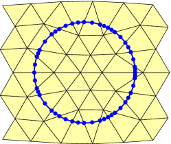
(a) meshes

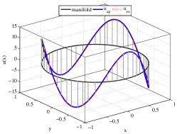
(b) exact solution

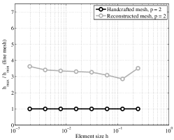
(c) ratio $h_{\mathrm{max}}/h_{\mathrm{min}}$

Figure 13: (a) Background and reconstructed line mesh for the circular manifold, (b) exact solution of the Poisson equation, (c) the largest ratio $h_{\mathrm{max}}/h_{\mathrm{min}}$ of the reconstructed line elements.

Fig. 14 shows the convergence rates and condition numbers. Fig. 14(a) and (c) are achieved on handcrafted meshes with equi-distant line elements. As expected, optimal convergence rates are seen in the $L_{2}$-norm and the condition number scales with $O\left(h^{2}\right)$. Fig. 14(b) and (d) show the corresponding results on the automatically generated meshes. The convergence rates are again optimal (the dotted lines show the optimal slope) and the condition numbers also scale with $O\left(h^{2}\right)$. Obviously, compared to the handcrafted meshes, the error level is modestly larger and the condition number is larger by about two order of magnitude.

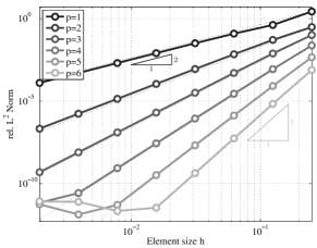
(a) handcr. mesh, $L_{2}$-norm

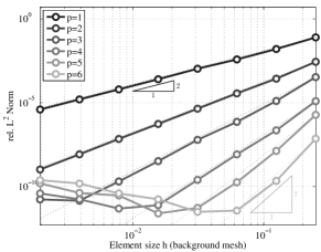
(b) recon. mesh, $L_{2}$-norm

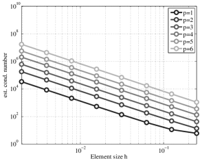
(c) handcr. mesh, cond.

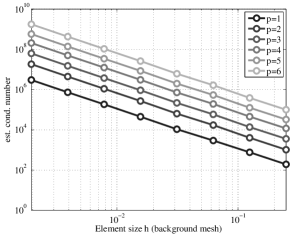
(d) recon. mesh, cond.

Figure 14: Convergence results and condition numbers for the Poisson equation on a circular manifold.

5.1.2 Flower-shaped manifold

Next, the Laplace-Beltrami operator is solved on a closed, flower-shaped manifold implied by the level-set function

$$\phi\left(\mathchoice{\displaystyle\boldsymbol{x}}{\textstyle\boldsymbol{x}}{\scriptstyle\boldsymbol{x}}{\scriptscriptstyle\boldsymbol{x}}\right)=\sqrt{x^{2}+y^{2}}-R\left(\theta\right),$$

with $R\left(\theta\right)=0.5+0.1\cdot\sin\left(8\theta\right)$ and $\theta\left(\mathchoice{\displaystyle\boldsymbol{x}}{\textstyle\boldsymbol{x}}{\scriptstyle\boldsymbol{x}}{\scriptscriptstyle\boldsymbol{x}}\right)=\mathrm{atan}\left(y/x\right)$. The function $u$ is defined as $u(\theta)=12\sin 3\theta$ and the right hand side is computed accordingly. See Fig. 15(a) for a coarse background mesh and a reconstructed line mesh of order $1$. The exact solution is seen in Fig. 15(b) and the largest ratio $h_{\mathrm{max}}/h_{\mathrm{min}}$ of the reconstructed line elements resulting from the different background meshes in Fig. 15(c).

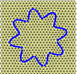
(a) meshes

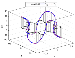
(b) exact solution

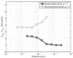
(c) ratio $h_{\mathrm{max}}/h_{\mathrm{min}}$

Figure 15: (a) Background and reconstructed line mesh for the flower-shaped manifold, (b) exact solution of the Poisson equation, (c) the largest ratio $h_{\mathrm{max}}/h_{\mathrm{min}}$ of the reconstructed line elements.

In the convergence studies, we use background meshes with $h=R/\left\{32,\,64,\,128,\,256,\,512,\,1024,\,2048\right\}$ which is fine enough to ensure that the reconstruction is successfully achieved without any (recursive/adaptive) refinements of the background elements. For the handcrafted meshes, significantly larger element lengths $h$ may be used. The results presented in Fig. 16 follow the same style than in the previous test case. It is confirmed that optimal convergence rates are achieved on handcrafted and automatically reconstructed meshes and the condition numbers behave as expected.

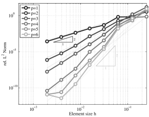
(a) handcr. mesh, $L_{2}$-norm

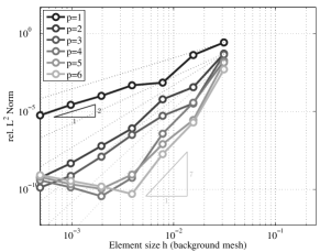
(b) recon. mesh, $L_{2}$-norm

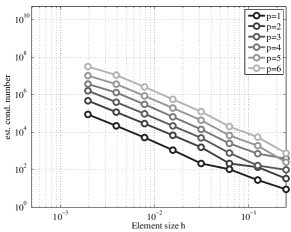
(c) handcr. mesh, cond.

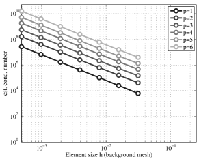
(d) recon. mesh, cond.

Figure 16: Convergence results and condition numbers for the Poisson equation on a flower-shaped manifold.

5.1.3 S-shaped manifold

In this example, we consider an open manifold where the boundary is defined by additional level-set functions $\psi^{i}\left(\mathchoice{\displaystyle\boldsymbol{x}}{\textstyle\boldsymbol{x}}{\scriptstyle\boldsymbol{x}}{\scriptscriptstyle\boldsymbol{x}}\right)$. The manifold in parametric form is given as

$$\Gamma=\begin{bmatrix}x\\ f(x)\end{bmatrix}=\begin{bmatrix}x\\ \frac{x^{3}}{2}+\sin(\pi(1-x))\sin^{5}\left(\frac{\pi}{2}(1-x)\right)-\frac{1}{4}\end{bmatrix}, \quad\mathrm{with}\;x\in\left[0,\,1\right].$$ (5.4)

The corresponding level-set function may be defined as

$$\phi(\mathchoice{\displaystyle\boldsymbol{x}}{\textstyle\boldsymbol{x}}{\scriptstyle\boldsymbol{x}}{\scriptscriptstyle\boldsymbol{x}})=f(x)-y\ .$$ (5.5)

The boundaries are defined by the two additional level-set functions $\psi^{1}(\mathchoice{\displaystyle\boldsymbol{x}}{\textstyle\boldsymbol{x}}{\scriptstyle\boldsymbol{x}}{\scriptscriptstyle\boldsymbol{x}})=\nicefrac{{1}}{{4}}-y$ and $\psi^{2}(\mathchoice{\displaystyle\boldsymbol{x}}{\textstyle\boldsymbol{x}}{\scriptstyle\boldsymbol{x}}{\scriptscriptstyle\boldsymbol{x}})=y-\nicefrac{{1}}{{4}}$. An example for a reconstructed line mesh is seen in Fig. 17(a) where also the zero-isolines of all three level-set functions are shown. The exact solution $u(\mathchoice{\displaystyle\boldsymbol{x}}{\textstyle\boldsymbol{x}}{\scriptstyle\boldsymbol{x}}{\scriptscriptstyle\boldsymbol{x}})=\exp\left(2x\right)$ is plotted in Fig. 17(b). Again, the ratio of the largest element length of the automatically reconstructed line mesh to the smallest is shown in Fig. 17(c). This ratio may be worse than in the previous examples due to the presence of several level-set functions which renders the manipulation of the background mesh more complicated.

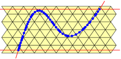
(a) meshes

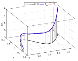
(b) exact solution

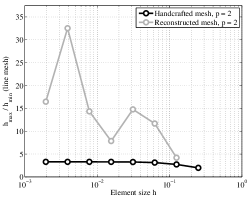
(c) ratio $h_{\mathrm{max}}/h_{\mathrm{min}}$

Figure 17: (a) Background and reconstructed line mesh for the S-shaped manifold, (b) exact solution of the Poisson equation, (c) the largest ratio $h_{\mathrm{max}}/h_{\mathrm{min}}$ of the reconstructed line elements.

In Fig. 18, the results of the convergence analysis is presented in the same style than above with the same conclusions to be drawn. Hence, we conclude that approximations of the Poisson equation with optimal convergence rates are possible for the automatically generated meshes discretizing closed and open curved lines in 2D.

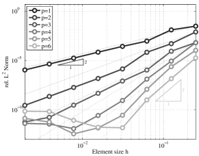
(a) handcr. mesh, $L_{2}$-norm

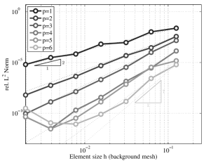
(b) recon. mesh, $L_{2}$-norm

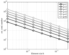
(c) handcr. mesh, cond.

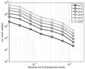
(d) recon. mesh, cond.

Figure 18: Convergence results and condition numbers for the Poisson equation on a S-shaped manifold.

5.2 Poisson equation on curved surfaces in 3D

5.2.1 Quarter Cylinder

Here, the Laplace-Beltrami operator is solved on the surface of a quarter cylinder with the radius $r=1$ and height $L=4$. The analytical solution in cylindrical coordinates $(r,\,\varphi,\,z)$ is given in [30] based on the following parameters and functions:

$$g_{\varphi,1}(\varphi) =\left(1-\cos\varphi\right)\left(1-\sin\varphi\right),$$ (5.6)

$$g_{\varphi,2}(\varphi) =\left(\cos\varphi+\sin\varphi-4\sin\varphi\cos\varphi\right),$$ (5.7)

$$g_{z}(z) =\sin\dfrac{\alpha\pi z}{L},$$ (5.8)

$$\alpha =3\,,\qquad\beta=\dfrac{1}{\frac{3}{2}-\sqrt{2}}\ .$$ (5.9)

The analytic solution is then defined as $u(r,\,\varphi,\,z)=\beta g_{\varphi,1}(\varphi)g_{z}(z)$. Applying the Laplace-Beltrami operator yields the source function

$$f=\beta\cdot g_{z}(z)\left[\left(\dfrac{\alpha\pi}{L}\right)^{2}g_{\varphi,1}(\varphi)-g_{\varphi,2}(\varphi)\right].$$

The Dirichlet boundary condition is $u\rvert_{\partial\Gamma_{\text{D}}}=0$. In this special case, it is particularly simple to use a tensor-product background mesh in the volume $\Omega=(0,r)\times(0,r)\times(0,L)$ to reconstruct the higher-order surface mesh with the desired boundaries. Hence, the use of addional level-set functions $\psi^{i}$ would unnecessarily complicate the situation here.

An example of a reconstructed, higher-order surface mesh is shown in Fig. 19(a). The exact solution is given in Fig. 19(b). The ratio of the largest surface element to the smallest is given in Fig. 19(c) and is, again, clearly bounded (in the range of $<20$ for this example).

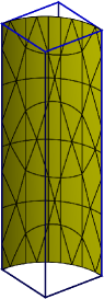
(a) Surface mesh

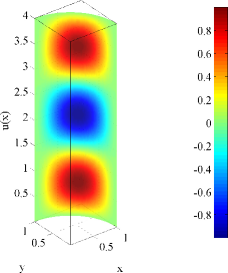
(b) exact solution

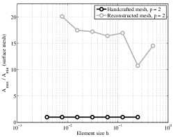
(c) ratio $A_{\mathrm{max}}/A_{\mathrm{min}}$

Figure 19: (a) Reconstructed surface mesh for the quarter cylinder, (b) exact solution of the Poisson equation, (c) the largest ratio $A_{\mathrm{max}}/A_{\mathrm{min}}$ of the reconstructed surface elements.

For the convergence studies we use background meshes with $h=r/\left\{4,\,8,\,16,\,32,\,64,\,128\right\}$ and results are shown in Fig. 18. As for the previous convergence studies for curved lines, Fig. 18(a) and (c) refer to convergence rates and condition numbers of handcrafted surface meshes, respectively. Fig. 18(b) and (d) give the results of the automatically generated surface meshes. The resulting convergence plots show optimal convergence rates which are surprisingly smooth given the irregularity of the reconstructed surface elements. The condition numbers are about two orders of magnitude larger than in the handcrafted meshes.

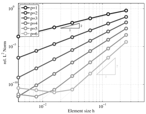
(a) handcr. mesh, $L_{2}$-norm

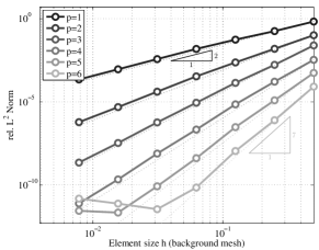
(b) recon. mesh, $L_{2}$-norm

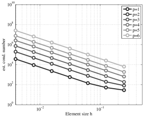
(c) handcr. mesh, cond.

(d) recon. mesh, cond.

Figure 20: Convergence results and condition numbers for the Poisson equation on a quarter cylinder.

5.2.2 Sphere

Next, we consider a sphere with radius $r=1$. Using spherical coordinates $(r,\,\varphi,\,\theta)$, an exact solution $u(r,\,\varphi,\,\theta)$ fulfilling the zero-mean constraint from Eq. (4.5) is chosen as

$$u(r,\,\varphi,\,\theta)=\sin(3\theta)\left(\cos\varphi-\sin\varphi\right)\ .$$ (5.10)

Applying the Laplace-Beltrami operator yields the source function

$$f=-\dfrac{2\sqrt{2}}{\sin(\theta)}\cos\left(\dfrac{\pi}{4}+\varphi\right)\,\left(24\cos^{4}\theta-29\cos^{2}\theta+5\right).$$ (5.11)

The test case is sketched in Fig. 21 showing (a) a reconstructed example mesh and (b) the exact solution on the sphere. The area ratios are given in Fig. 21(c). In Fig. 22, convergence results and condition numbers are only shown for the automatically reconstructed surface meshes because the findings coincide with the previous test case. It is well-known that the inner angles in the elements play an important role for the quality of a mesh. In particular, large inner angles may hinder optimal convergence [15]. Therefore, for all meshes the maximum inner angles have also been computed. The generated meshes are typically mixed, i.e., composed by quadrilateral and triangular elements and the maximum angles have been computed for these two element types individually. Results are shown in Fig. 23 for first order and $6$th-order meshes only because all other orders yield very similar results. As can be seen the maximum inner angles in quadrilaterals are below $140^{\circ}$ and in triangles below $110^{\circ}$. This was also confirmed in the other test cases where one level-set function defines the manifold.

(a) Surface mesh

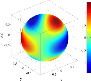
(b) exact solution

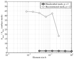
(c) ratio $A_{\mathrm{max}}/A_{\mathrm{min}}$

Figure 21: (a) Reconstructed surface mesh for the sphere, (b) exact solution of the Poisson equation, (c) the largest ratio $A_{\mathrm{max}}/A_{\mathrm{min}}$ of the reconstructed surface elements.

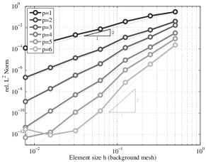
(a) recon. mesh, $L_{2}$-norm

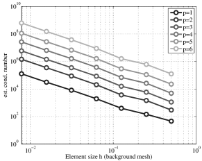
(b) recon. mesh, cond.

Figure 22: Convergence results and condition numbers for the Poisson equation on a sphere.

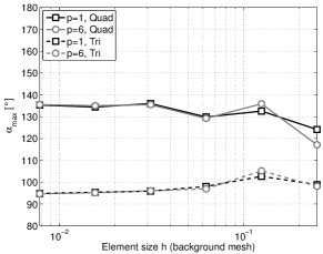
Figure 23: Maximum inner angles of the automatically generated meshes of the sphere.

5.2.3 Hyperbolic paraboloid with bumps

Now we consider the Laplace-Beltrami operator on a hyperbolic paraboloid with bumps. The surface is defined by the function

$$f\left(x,y\right)=\dfrac{1}{2}\left(x^{2}-y^{2}\right)+\dfrac{3}{20}\sin\left(2\pi x\right)\sin\left(2\pi y\right)$$

with $x,y\in\left[-0.5,0.5\right]$. The analytic solution $u$ is chosen as

$$u(x,y)=\sin\left[\pi\left(x-\dfrac{1}{2}\right)\right]\,\sin\left[\pi\left(y-\dfrac{1}{2}\right)\right]$$ (5.12)

and the source function $f$ determined accordingly. The level-set function $\phi\left(\mathchoice{\displaystyle\boldsymbol{x}}{\textstyle\boldsymbol{x}}{\scriptstyle\boldsymbol{x}}{\scriptscriptstyle\boldsymbol{x}}\right)$ implying the manifold is

$$\phi(\mathchoice{\displaystyle\boldsymbol{x}}{\textstyle\boldsymbol{x}}{\scriptstyle\boldsymbol{x}}{\scriptscriptstyle\boldsymbol{x}})=f(x,y)-z\ .$$ (5.13)

If the reconstruction is achieved based on a cube-like background mesh with suitable dimensions, the manipulation of the background mesh is restricted in that nodes on the outer contour of the background mesh cannot be moved freely without changing the boundary $\partial\Gamma$ of the implied manifold. Therefore, we use four additional level-set functions $\psi^{i}\left(\mathchoice{\displaystyle\boldsymbol{x}}{\textstyle\boldsymbol{x}}{\scriptstyle\boldsymbol{x}}{\scriptscriptstyle\boldsymbol{x}}\right)$ which restrict the manifold properly. The mesh manipulation of the (universal) background mesh, see Section 2, is then applied with respect to all level-set functions and the element ratios are sufficently bounded.

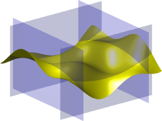
(a) Zero-level sets

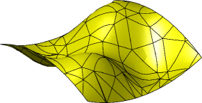
(b) Surface mesh

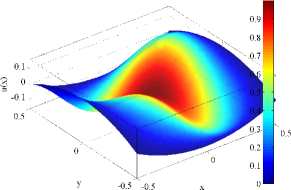
(c) exact solution

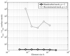
(d) ratio $A_{\mathrm{max}}/A_{\mathrm{min}}$

Figure 24: (a) Zero iso-surfaces of $\phi$ and $\psi^{i}$, (b) reconstructed surface mesh for the hyperbolic paraboloid with bumps, (c) exact solution of the Poisson equation, (d) the largest ratio $A_{\mathrm{max}}/A_{\mathrm{min}}$ of the reconstructed surface elements.

The additional level-set functions are

$$\psi^{i}(\mathchoice{\displaystyle\boldsymbol{x}}{\textstyle\boldsymbol{x}}{\scriptstyle\boldsymbol{x}}{\scriptscriptstyle\boldsymbol{x}}) =\left\langle\mathchoice{\displaystyle\boldsymbol{x}}{\textstyle\boldsymbol{x}}{\scriptstyle\boldsymbol{x}}{\scriptscriptstyle\boldsymbol{x}}-\mathchoice{\displaystyle\boldsymbol{P}}{\textstyle\boldsymbol{P}}{\scriptstyle\boldsymbol{P}}{\scriptscriptstyle\boldsymbol{P}}_{i},\,\mathchoice{\displaystyle\boldsymbol{n}}{\textstyle\boldsymbol{n}}{\scriptstyle\boldsymbol{n}}{\scriptscriptstyle\boldsymbol{n}}_{i}\right\rangle\qquad i=1,\,\ldots,\,4$$

where $\left\langle\;,\;\right\rangle$ is a scalar product and

$$\mathchoice{\displaystyle\boldsymbol{P}}{\textstyle\boldsymbol{P}}{\scriptstyle\boldsymbol{P}}{\scriptscriptstyle\boldsymbol{P}}_{1} =\left[\begin{array}[]{c}0.5\\ 0\\ 0\end{array}\right]\quad \mathchoice{\displaystyle\boldsymbol{P}}{\textstyle\boldsymbol{P}}{\scriptstyle\boldsymbol{P}}{\scriptscriptstyle\boldsymbol{P}}_{2} =\left[\begin{array}[]{c}0\\ 0.5\\ 0\end{array}\right]\quad \mathchoice{\displaystyle\boldsymbol{P}}{\textstyle\boldsymbol{P}}{\scriptstyle\boldsymbol{P}}{\scriptscriptstyle\boldsymbol{P}}_{3} =\left[\begin{array}[]{c}-0.5\\ 0\\ 0\end{array}\right]\quad \mathchoice{\displaystyle\boldsymbol{P}}{\textstyle\boldsymbol{P}}{\scriptstyle\boldsymbol{P}}{\scriptscriptstyle\boldsymbol{P}}_{4} =\left[\begin{array}[]{c}0\\ -0.5\\ 0\end{array}\right]$$

$$\mathchoice{\displaystyle\boldsymbol{n}}{\textstyle\boldsymbol{n}}{\scriptstyle\boldsymbol{n}}{\scriptscriptstyle\boldsymbol{n}}_{1} =\left[\begin{array}[]{c}1\\ 0\\ 0\end{array}\right] \mathchoice{\displaystyle\boldsymbol{n}}{\textstyle\boldsymbol{n}}{\scriptstyle\boldsymbol{n}}{\scriptscriptstyle\boldsymbol{n}}_{2} =\left[\begin{array}[]{c}0\\ 1\\ 0\end{array}\right] \mathchoice{\displaystyle\boldsymbol{n}}{\textstyle\boldsymbol{n}}{\scriptstyle\boldsymbol{n}}{\scriptscriptstyle\boldsymbol{n}}_{3} =\left[\begin{array}[]{c}-1\\ 0\\ 0\end{array}\right] \mathchoice{\displaystyle\boldsymbol{n}}{\textstyle\boldsymbol{n}}{\scriptstyle\boldsymbol{n}}{\scriptscriptstyle\boldsymbol{n}}_{4} =\left[\begin{array}[]{c}0\\ -1\\ 0\end{array}\right]$$

The resulting zero-level sets are planes restricting the zero-level set $\Gamma_{\phi}$ implied by Eq. (5.13). See Fig. 24(a) for a visualization of the zero-level sets and (b) the resulting bounded manifold. Fig. 24(c) and (d) show the exact solution and the area ratios of the resulting surface elements, respectively. Convergence results and condition numbers for the automatically reconstructed meshes are seen in Fig. 25.

(a) recon. mesh, $L_{2}$-norm

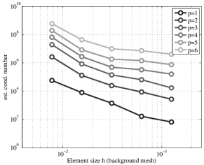
(b) recon. mesh, cond.

Figure 25: Convergence results and condition numbers for the Poisson equation on a hyperbolic paraboloid with bumps.

5.3 Instationary transport equation in 2D and 3D

The instationary advection-diffusion equation on manifolds is considered here. The semi-discrete weak form is given in Eq. (4.11). The time discretization is carried out using a $6$th-order accurate, implicit, $3$-step Runge-Kutta method as defined in Eq. (4.12). We use a constant number of 4096 time steps in all upcoming examples which virtually eliminates the discretization error in time. First, we consider pure advection problems on a circle and a sphere, i.e. without any diffusion. Then, two test cases are considered with diffusion where no analytic solution is available. In the error studies, the $L_{2}$-error is measured in space at the final time step. Of course, this error is effected by the discretizations in space and time, wherefore we employ the highly accurate time stepping scheme mentioned above.

5.3.1 Pure advection on a circular manifold

The instationary transport problem is solved on a circle with radius $r=1$ in the time interval $t\in(0,1)$. The advection velocity is $\left\|\mathchoice{\displaystyle\boldsymbol{c}}{\textstyle\boldsymbol{c}}{\scriptstyle\boldsymbol{c}}{\scriptscriptstyle\boldsymbol{c}}_{\Gamma}\right\|=5$ in tangential direction of the circle and the diffusion coefficient $\lambda=0$. The initial condition is

$$u_{0}(\mathchoice{\displaystyle\boldsymbol{x}}{\textstyle\boldsymbol{x}}{\scriptstyle\boldsymbol{x}}{\scriptscriptstyle\boldsymbol{x}})=\exp\left(-4\cdot\varphi\left(\mathchoice{\displaystyle\boldsymbol{x}}{\textstyle\boldsymbol{x}}{\scriptstyle\boldsymbol{x}}{\scriptscriptstyle\boldsymbol{x}}\right)^{2}\right)\ \mathrm{with}\;\varphi=\mathrm{atan}\left(y/x\right),\;\varphi\in\left[-\pi,\,\pi\right],\ \mathchoice{\displaystyle\boldsymbol{x}}{\textstyle\boldsymbol{x}}{\scriptstyle\boldsymbol{x}}{\scriptscriptstyle\boldsymbol{x}}\in\Gamma.$$ (5.14)

This initial distribution is simply advected around the circle without changing its shape. That is, the exact solution is (5.14) with a shift in the angle of $\Delta\varphi=\left\|\mathchoice{\displaystyle\boldsymbol{c}}{\textstyle\boldsymbol{c}}{\scriptstyle\boldsymbol{c}}{\scriptscriptstyle\boldsymbol{c}}_{\Gamma}\right\|/r\cdot t$. See Fig. 26 for a graphical representation of the solution at different instances in time at $t=\left[0.00,\,0.20,\,1.00\right]$.

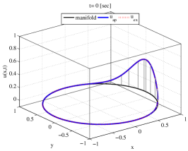
(a) Initial state

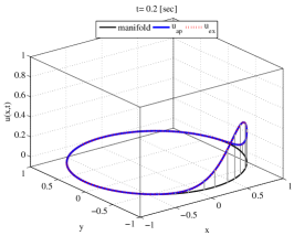
(b) State at $0.20$

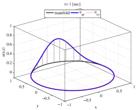
(c) State at $1.00$

Figure 26: Solution of the instationary transport problem on a circle without diffusion.

For this study, the same meshes from Section 5.1.1 are used. Results are presented in Fig. 27 in the same style than above. It is seen that higher-order convergence rates are achieved. However, for this pure advection problem, one order of the optimal convergence rate is lost for even orders of the elements, i.e. $p=2,4,6,\dots$ This is the same for handcrafted meshes as well as for the automatically reconstructed meshes. We have confirmed that the same behavior also occurs for planar advection problems so this has nothing to do with the fact that the problem is solved on a curved manifold nor that no boundaries are present.

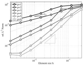
(a) handcr. mesh, $L_{2}$-norm

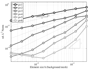
(b) recon. mesh, $L_{2}$-norm

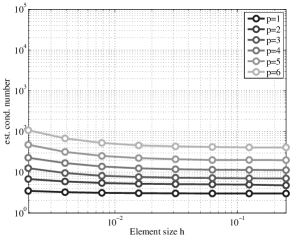
(c) handcr. mesh, cond.

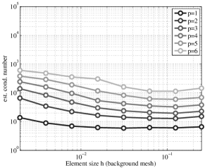
(d) recon. mesh, cond.

Figure 27: Convergence results and condition numbers for the transport equation on a circular manifold.

5.3.2 Pure advection on a sphere

A similar problem without diffusion is now solved on a sphere with radius $r=1$ in the time interval $t\in(0,1)$. The advection velocity is

$$\mathchoice{\displaystyle\boldsymbol{c}}{\textstyle\boldsymbol{c}}{\scriptstyle\boldsymbol{c}}{\scriptscriptstyle\boldsymbol{c}}_{\Gamma}=\left[\begin{array}[]{c}c_{x}\\ 0\\ c_{z}\end{array}\right]=\left[\begin{array}[]{c}z\\ 0\\ -x\end{array}\right]\cdot\frac{c}{r},\quad c=-\frac{7}{8}$$

taking place only in the $xz$-plane tangential to the sphere. The initial state is set to

$$u_{0}(\mathchoice{\displaystyle\boldsymbol{x}}{\textstyle\boldsymbol{x}}{\scriptstyle\boldsymbol{x}}{\scriptscriptstyle\boldsymbol{x}})=\exp\left(-4\theta(\mathchoice{\displaystyle\boldsymbol{x}}{\textstyle\boldsymbol{x}}{\scriptstyle\boldsymbol{x}}{\scriptscriptstyle\boldsymbol{x}})^{2}\right)\ \mathrm{with}\;\theta=\mathrm{acos}\left(z/r\right),\ \theta\in\left[0,\,\pi\right],\ \mathchoice{\displaystyle\boldsymbol{x}}{\textstyle\boldsymbol{x}}{\scriptstyle\boldsymbol{x}}{\scriptscriptstyle\boldsymbol{x}}\in\Gamma.$$ (5.15)

Analogously to the example above, the exact solution is obtained by the rotation angle in the $xz$-plane. In Fig. 28, the analytical solution at $t=\left[0.00,\,0.50,\,1.00\right]$ is illustrated.

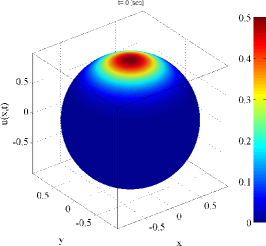
(a) Initial state

(b) State at $0.50\,\text{s}$

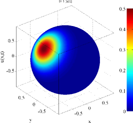
(c) State at $1.00\,\text{s}$

Figure 28: Solution of the instationary transport problem on a sphere without diffusion.

The same meshes from Section 5.2.2 are used and results are seen in Fig. 29. The same conclusions from above may be drawn, in particular the loss of one order in the convergence rate for elements with even orders. It is recalled that this behaviour is typical for pure advection and optimal convergence rates are recovered in the presence of diffusion. This is equivalent to results of planar problems with handcrafted meshes.

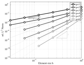
(a) handcr. mesh, $L_{2}$-norm

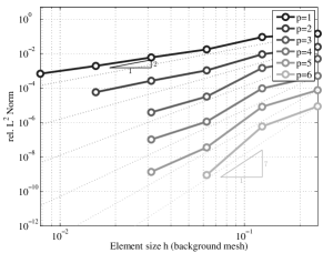
(b) recon. mesh, $L_{2}$-norm

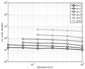
(c) handcr. mesh, cond.

(d) recon. mesh, cond.

Figure 29: Convergence results and condition numbers for the transport equation on a sphere.

5.3.3 Advection-diffusion on an S-shaped manifold

Next, the instationary transport problem is solved on the S-shaped manifold of Section 5.1.3 in the time interval $t\in(0,1)$. The advection velocity is $\left\|\mathchoice{\displaystyle\boldsymbol{c}}{\textstyle\boldsymbol{c}}{\scriptstyle\boldsymbol{c}}{\scriptscriptstyle\boldsymbol{c}}_{\Gamma}\right\|=1$ and the diffusion coefficient $\lambda=0.15$. A Dirichlet boundary condition of $u=1$ is prescribed at the inflow. The initial condition is $u=0$ everywhere on $\Gamma$. As there is no analytical solution available, no convergence study is performed and only a representative approximation is shown in Fig. 30.

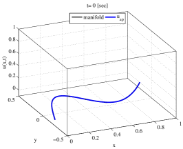
(a) Initial state

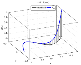
(b) State at $0.19$

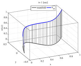
(c) State at $1.00$

Figure 30: Solution of an instationary transport problem on an S-shaped manifold.

5.3.4 Advection-diffusion on a hyperbolic paraboloid with bumps

Finally, an advection-diffusion problem is considered on the hyperbolic paraboloid with bumps introduced in Section 5.2.3. The time interval is again $t\in(0,1)$, the advection velocity $\left\|\mathchoice{\displaystyle\boldsymbol{c}}{\textstyle\boldsymbol{c}}{\scriptstyle\boldsymbol{c}}{\scriptscriptstyle\boldsymbol{c}}_{\Gamma}\right\|=1.25$ tangential to the manifold in the direction of $y$, and the diffusion coefficient $\lambda=0.01$. The initial condition is given by $u(\mathchoice{\displaystyle\boldsymbol{x}}{\textstyle\boldsymbol{x}}{\scriptstyle\boldsymbol{x}}{\scriptscriptstyle\boldsymbol{x}},0)=\dfrac{1}{2}\exp\left[-10\left(x^{2}+y^{2}\right)\right]$. A representative result is seen in Fig. 31.

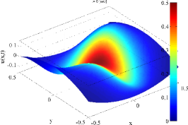
(a) Initial state

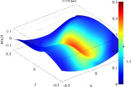
(b) State at $0.49$

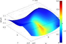
(c) State at $1.00$

Figure 31: Solution of an instationary transport problem on a hyperbolic parabolid with bumps.

6 Conclusions

A higher-order accurate method for PDEs on surfaces is proposed. It enables a completely automatic workflow from the geometric description based on level-sets to the numerical analysis without any user-intervention. This is an important advantage over other methods which are based on handcrafted surface meshes. Furthermore, these meshes are often composed by flat triangles leading to a low-order representation of the geometry and the resulting approximation of the BVP. Compared to methods which solve BVPs on all zero-isosurfaces at once by using volumetric elements, the proposed approach is more efficient as the effort scales with standard planar, two-dimensional BVPs. Compared to methods which employ shape functions of the background mesh as in TraceFEM and CutFEM, it is an important advantage that boundary conditions are enforced in the standard way without additional technqiues for general constraints (Lagrange multipliers, Nitsche’s method etc.).

The proposed method is characterized by the following key ingredients:

1. A geometry description of the bounded manifold based on several level-set functions.

2. The automatic generation of surface elements which enable a $C_{0}$-continuous, higher-order accurate representation of the level-set geometry. A conforming surface mesh used for the finite element approximation is automatically extracted from this set of surface elements.

3. The manipulation of the background mesh by node movements in order to ensure the shape regularity of the resulting surface elements and a bounded condition number of the resulting system of equations. This step may later be replaced by a stabilization similar to what is done in the TraceFEM and CutFEM.

The numerical results confirm that higher-order accurate solutions of BVPs on curved surfaces in three dimensions are achieved. The next steps will be to investigate the proposed technique for the solution of more advanced BVPs on manifolds such as flow problems on curved surfaces and the numerical analysis of membranes and shells.

References

- [1] Adalsteinsson, D.; Sethian, J.A.: Transport and diffusion of material quantities on propagating interfaces via level set methods. J. Comput. Phys., 185, 271 – 288, 2003.
- [2] Bertalmio, M.; Cheng, L.T.; Osher, S.; Sapiro, G.: Variational problems and partial differential equations on implicit surfaces: The framework and examples in image processing and pattern formation. J. Comput. Phys., 174, 759 – 780, 2001.
- [3] Blaauwendraad, J.; Hoefakker, J.H.: Structural Shell Analysis, Vol. 200, Solid Mechanics and Its Applications. Springer, Berlin, 2014.
- [4] Burger, M.: Finite element approximation of elliptic partial differential equations on implicit surfaces. Computing and Visualization in Science, 12, 87 – 100, 2009.
- [5] Burman, E.; Hansbo, P.; Larson, M.G.: A stabilized cut finite element method for partial differential equations on surfaces: The Laplace-Beltrami operator. Comp. Methods Appl. Mech. Engrg., 285, 188 – 207, 2015.
- [6] Burman, E.; Hansbo, P.; Larson, M.G.; Larsson, K.; Massing, A.: Finite Element Approximation of the Laplace-Beltrami Operator on a Surface with Boundary. ArXiv e-prints, Sep 2015.
- [7] Chapelle, D.; Bathe, K.J.: The Finite Element Analysis of Shells – Fundamentals. Computational Fluid and Solid Mechanics. Springer, Berlin, 2011.
- [8] Deckelnick, K.; Dziuk, G.; Elliott, C.M.; Heine, C.J.: An -narrow band finite-element method for elliptic equations on implicit surfaces. IMA Journal of Numerical Analysis, 30, 351 – 376, 2010.
- [9] Deckelnick, K.; Elliott, C.M.; Ranner, T.: Unfitted finite element methods using bulk meshesfor surface partial differential equations. SIAM J. Numer. Anal., 52, 2137 – 2162, 2014.
- [10] Delfour, M.C.; Zolésio, J.P.: A Boundary Differential Equation for Thin Shells. Journal of Differential Equations, 119, 426 – 449, 1995.
- [11] Delfour, M.C.; Zolésio, J.P.: Tangential Differential Equations for Dynamical Thin-Shallow Shells. Journal of Differential Equations, 128, 125 – 167, 1996.
- [12] Demlow, A.: Higher-order finite element methods and pointwise error estimates for elliptic problems on surfaces. SIAM J. Numer. Anal., 47, 805 – 827, 2009.
- [13] Demlow, A.; Dziuk, G.: An adaptive finite element method for the Laplace-Beltrami operator on implicitly defined surfaces. SIAM J. Numer. Anal., 45, 421 – 442, 2007.
- [14] Demlow, A.; Olshanskii, M.A.: An adaptive surface finite element method based on volume meshes. SIAM J. Numer. Anal., 50, 1624 – 1647, 2012.
- [15] Deuflhard, P.; Weiser, M.: Adaptive numerical solutions of PDEs. De Gruyter, Berlin, 2012.
- [16] Du, Q.; Ju, L.; Tian, L.: Finite element approximation of the Cahn-Hilliard equation on surfaces. Comp. Methods Appl. Mech. Engrg., 200, 2458 – 2470, 2011.
- [17] Dziuk, G.: Finite Elements for the Beltrami operator on arbitrary surfaces, Chapter 6, 142 – 155. Springer Berlin Heidelberg, Berlin, Heidelberg, 1988.
- [18] Dziuk, G.; Elliott, C.M.: Finite elements on evolving surfaces. IMA Journal of Numerical Analysis, 27, 262 – 292, 2007.
- [19] Dziuk, G.; Elliott, C.M.: Eulerian finite element method for parabolic PDEs and on implicit surfaces. Interfaces and Free Boundaries, 10, 2008.
- [20] Dziuk, G.; Elliott, C.M.: Finite element methods for surface PDEs. Acta Numerica, 22, 289 – 396, 2013.
- [21] Elliott, C.M.; Stinner, B.: Analysis of a diffuse interface approach to an advection diffusion equation on a moving surface. Mathematical Models and Methods in Applied Sciences, 19, 787 – 802, 2009.
- [22] Elliott, C.M.; Styles, V.: An ALE ESFEM for Solving PDEs on Evolving Surfaces. Milan Journal of Mathematics, 80, 469 – 501, 2012.
- [23] Fries, T.P.; Omerović, S.: Higher-order accurate integration of implicit geometries. Internat. J. Numer. Methods Engrg., 106, 323 – 371, 2016.
- [24] Fries, T.P.; Omerović, S.; Schöllhammer, D.; Steidl, J.: Higher-order meshing of implicit geometries—part I: Integration and interpolation in cut elements. Comp. Methods Appl. Mech. Engrg., 313, 759 – 784, 2017.
- [25] Grande, J.; Reusken, A.: A Higher Order Finite Element Method for Partial Differential Equations on Surfaces. SIAM J. Numer. Anal., 54, 388 – 414, 2016.
- [26] Gross, S.; Reusken, A.: Numerical Methods for Two-phase Incompressible Flows, Vol. 40, Springer Series in Computational Mathematics. Springer, Berlin, 2011.
- [27] Hansbo, A.; Hansbo, P.: A finite element method for the simulation of strong and weak discontinuities in solid mechanics. Comp. Methods Appl. Mech. Engrg., 193, 3523 – 3540, 2004.
- [28] Hansbo, P.; Larson, M.G.: Finite element modeling of a linear membrane shell problem using tangential differential calculus. Comp. Methods Appl. Mech. Engrg., 270, 1 – 14, 2014.
- [29] Hansbo, P.; Larson, M.G; Larsson, F.: Tangential differential calculus and the finite element modeling of a large deformation elastic membrane problem. Comput. Mech., 56, 87 – 95, 2015.
- [30] Kamilis, D.: Numerical methods for the PDEs on curves and surfaces. Masters thesis, Umeå university, Umeå, Sweden, 2013.
- [31] Olshanskii, M.A.; Reusken, A.: A finite element method for surface PDEs: matrix properties. Numer. Math., 114, 491 – 520, 2010.
- [32] Olshanskii, M.A.; Reusken, A.; Grande, J.: A finite element method for elliptic equations on surfaces. SIAM J. Numer. Anal., 47, 3339 – 3358, 2009.
- [33] Olshanskii, M.A.; Reusken, A.; Xu, X.: On surface meshes induced by level set functions. Comput. Visual Sci., 15, 53 – 60, 2012.
- [34] Olshanskii, M.A.; Reusken, A.; Xu, X.: A stabilized finite element method for advection-diffusion equations on surfaces. IMA Journal of Numerical Analysis, 34(2), 732 – 758, 2014.
- [35] Olshanskii, M.A.; Safin, D.: Numerical integration over implicitly defined domains for higher order unfitted finite element methods. Lobachevskii Journal of Mathematics, 37, 582 – 596, 2016.
- [36] Rangarajan, R.; Lew, A.J.: Universal Meshes: A new paradigm for computing with nonconforming triangulations. arxiv:1201.4903, 2012.
- [37] Rätz, A.; Voigt, A.: PDEs on surfaces – A diffuse interface approach. Communications in Mathematical Sciences, 4, 575 – 590, 2006.
- [38] Reusken, A.: Analysis of trace finite element methods for surface partial differential equations. IMA J Numer Anal, 35, 1568 – 1590, 2014.
- [39] Xu, J.J.; Yang, Y.; Lowengrub, J.: A level-set continuum method for two-phase flows with insoluble surfactant. J. Comput. Phys., 231, 5897 – 5909, 2012.
- [40] Xu, J.J.; Zhao, H.K.: An Eulerian Formulation for Solving Partial Differential Equations along a Moving Interface. Journal of Scientific Computing, 19, 573 – 594, 2003.