COMPARATIVE PERFORMANCE ANALYSIS OF THE CUMULATIVE SUM CHART AND THE SHIRYAEV–ROBERTS PROCEDURE FOR DETECTING CHANGES IN AUTOCORRELATED DATA

Abstract

We consider the problem of quickest change-point detection where the observations form a first-order autoregressive (AR) process driven by temporally independent standard Gaussian noise. Subject to possible change are both the drift of the AR(1) process ($\mu$) as well as its correlation coefficient ($\lambda$), both known. The change is abrupt and persistent, and is of known magnitude, with $\left|\lambda\right|<1$ throughout. For this scenario, we carry out a comparative performance analysis of the popular Cumulative Sum (CUSUM) chart and its less well-known but worthy competitor—the Shiryaev–Roberts (SR) procedure. Specifically, the performance is measured through Pollak’s Supremum (conditional) Average Delay to Detection (SADD) constrained to a pre-specified level of the Average Run Length (ARL) to false alarm. Particular attention is drawn to the sensitivity of each procedure’s SADD and ARL with respect to the value of $\lambda$ before and after the change. The performance is studied through the solution of the respective integral renewal equations obtained via Monte Carlo simulations. The simulations are designed to estimate the sought performance metrics in an unbiased and asymptotically strongly consistent manner, and to within a prescribed proportional closeness (also asymptotically). Our extensive numerical studies suggest that both the CUSUM chart and the SR procedure are asymptotically second-order optimal, even though the CUSUM chart is found to be slightly better than the SR procedure, irrespective of the model parameters. Moreover, the existence of a worst-case post-change correlation parameter corresponding to the poorest detectability of the change for a given ARL to false alarm is established as well. To the best of our knowledge, this is the first time the performance of the SR procedure is studied for autocorrelated data.

refcheckUnused label ‘sec:intro’

url]http://people.math.binghamton.edu/aleksey

1 Introduction

Sequential (quickest) change-point detection is concerned with the design and analysis of reliable statistical machinery for quick detection of potential changes in the attributes of a random process. Specifically, the process is assumed to be continuously monitored through observations made sequentially, and should their behavior suggest that the process may have statistically changed, the aim is to conclude so within the fewest observations possible, subject to a tolerance level on the risk of false alarm. A sequential change-point detection procedure is a stopping-time adapted to the observations, and provides a rule to stop and declare that a change may be in effect. This problem finds applications in many branches of science and engineering: quality control, biostatistics, economics, seismology, and communication systems; see, e.g., [1, 2, 3].

In the simplest change-point detection problem, the observations are independent and identically distributed (i.i.d.) with known pre- and post-change distributions. In this setting, the problem is well-understood and has been solved to optimize different objectives. For a recent survey, see [4, 5] and references therein. In general, two solutions stand out: Page’s Cumulative Sum (CUSUM) chart [6] and the Shiryaev–Roberts (SR) procedure due to the independent work of Shiryaev [7, 8] and Roberts [9]. While the two procedures are statistically different, both are optimal under different sets of criteria. In particular, Moustakides [10] and Ritov [11] have shown that the CUSUM chart is exactly minimax-optimal in the sense of minimizing the detection delay under the most unfavorable set of observations and change-point. This type of minimax optimality was proposed by Lorden [12]. On the other hand, Pollak and Tartakovsky [13] showed that the SR procedure is optimal in the stationary setting, a scenario more suitable for detecting changes that occur at a distant time-horizon. Given that the Lorden criterion is often conservative, Pollak and Siegmund [14] introduced a more reasonable metric of detection delay under the most unfavorable change-point, but averaged over the observations; see also [15]. While the structure of the exactly optimal solution is unknown for the Pollak criterion, both the CUSUM chart and SR procedure are asymptotically optimal as the false alarm risk vanishes; see, e.g., [16]. Thus, there has been a good justification for comparing the two procedures with each other.

This comparative analysis has been done extensively in the i.i.d. case and we now present a brief sampling of this literature. The study in [17] offered a comprehensive asymptotic analysis (in the low false alarm regime) for the problem of detecting a change in the drift of Brownian motion. The conclusion in [17] was that the CUSUM chart is better for changes that occur in the beginning, whereas the SR procedure out-performs the CUSUM chart for change at infinity. Dragalin [18] developed an accurate numerical technique to capture the performance of the CUSUM chart in detecting a change in the mean of a Gaussian sequence. More recently, Moustakides et. al [19, 20] have developed an exact analytical characterization of the two procedures under either criteria through a set of integral-equations. These equations are in turn solved numerically using simple computational techniques. Confirming the findings of Pollak and Siegmund [17] and Pollak and Tartakovsky [13], these computations show that the CUSUM chart is superior to the SR procedure under the Pollak criterion, whereas the SR procedure is better in the stationary sense.

Despite the strong theoretical focus on the i.i.d. problem, observations are often serially correlated in industrial practice with a first-order autoregressive (AR(1)) process model being a good fit in many scenarios. A change could occur either due to a shift in the mean level or in the correlation coefficient (of the AR process) or both attributes simultaneously; see different examples in [1, 2, 21, 22, 23, 24], etc. Many works in the literature have shown that when the traditional Shewhart, Exponentially Weighted Moving Average (EWMA) and CUSUM charts designed for i.i.d. observations are used with AR processes, they result in seriously misleading conclusions; e.g., see typical case-studies in [25, 26, 27].

Motivated by these observations, modified versions of the traditional control charts accommodating serial correlations have been proposed; see [28, 25, 23, 29, 30, 31, 32] for some extensions along these lines. Most of these procedures decompose the correlated data into common cause effects and residuals (innovations) that are mutually independent. Under certain assumptions, the statistical properties of the residuals can be characterized. Specifically, the limiting distribution of the likelihood ratio function under either a mean shift or a correlation change in the AR process has been studied and various approximations to the average run length (ARL) to false alarm are obtained in [33, 34, 35, 29, 36, 37, 38, 39, 40, 41]. In particular, Davis, Huang, and Yao [42] has shown that the likelihood ratio statistic converges weakly to the extreme value distribution and use this property to characterize the performance of the CUSUM chart, whereas Timmer et. al [43] estimate the ARL of the CUSUM chart using a Markov chain representation. The studies in [44] and [45] use the efficient score vector representation of the likelihood ratio statistic of weighted CUSUM charts to characterize their performance.

In spite of this vast literature, optimality properties of the CUSUM chart have been explored only under certain special settings and only up to first-order. For example, Moustakides [46] has shown that the CUSUM test statistic reduces to the i.i.d. statistic in the special case where only the mean of the AR process changes and the CUSUM chart is thus optimal in the Lorden sense. First-order optimality of the CUSUM chart and the SR procedure under more general observation models has also been established; see e.g., [47, 48] and [16]. First-order optimality of the CUSUM chart under certain general change-point models relevant in practice is explored in [49]. Nevertheless, a comparative performance of the CUSUM chart with the SR procedure in the model parameter space has not been explored in the AR setting in full generality. The focus of this paper is on this task and we provide a comparative study of the two procedures in the non-asymptotic setting with correlated observations. We are not aware of any similar prior work in this area.

This paper is organized as follows. In Section 2, we set the backdrop for this paper by elaborating on the problem set-up, developing the notation, and connecting it with prior results in this area. In Section 3, the KL number between autoregressive processes is studied as a function of the pre- and post-change model parameters. In Section 4, we derive the integral equations for the performance metrics of interest and provide a simple numerical solution that allows for efficient computation of the operating characteristics. In Section 5, we present the results of our numerical studies and discuss the findings. Section 6 summarizes and concludes the paper.

2 Problem Formulation and Preliminary Background

The aim of this section is to formally state the problem, present the CUSUM chart and the Shiryaev–Roberts (SR) procedure, both set up appropriately, and review their (asymptotic) optimality properties.

Let $\{X_{n}\}_{n\geq 0}$ be an observation sequence formed sequentially from the output of an AR(1) process driven by temporally-independent standard Gaussian noise $\{\varepsilon_{n}\}_{n\geq 1}$, i.e., $\varepsilon_{n}\sim\mathcal{N}(0,1)$, $n\geq 1$, and $\varepsilon_{i}$ is independent of $\varepsilon_{j}$ if $i\neq j$. Let the statistical nature of the observation sequence, $\{X_{n}\}_{n\geq 0}$, be temporally piece-wise:

$$X_{n} =\begin{cases}\mu_{\infty}+\lambda_{\infty}X_{n-1}+\varepsilon_{n},\;\text{for $1\leq n\leq\nu$;}\\ \mu_{0}+\lambda_{0}X_{n-1}+\varepsilon_{n},\;\text{for $n\geq\nu+1$},\end{cases}$$ (1)

where $\mu_{d}\in\mathbb{R}$ and $\lambda_{d}$ is such that $\left|\lambda_{d}\right|<1$. $\mu_{d}$ and $\lambda_{d}$ are known for both $d=\{0,\infty\}$, $X_{0}=x_{0}\in\mathbb{R}$ is a given deterministic value, and $\nu$ is a parameter discussed next. The data model in (1) says that the observation sequence, $\{X_{n}\}_{n\geq 0}$, as it is formed in a one-observation-at-a-time manner, undergoes a spontaneous change in its statistical nature. The quickest change-point detection problem is to as quickly and reliably as possible establish that the statistical nature has changed. The challenge is that the time instance $\nu$, which is referred to as the change-point, is not known in advance. A solution to the problem is a detection procedure identified with a $\{X_{n}\}_{n\geq 0}$-adapted stopping time, $T$, and a “good” procedure is one whose detection delay cost is the smallest possible within a given tolerable range of the false alarm risk.

Remark.

A noteworthy feature of the AR(1) model in (1) is that $X_{0},X_{1},\cdots,X_{\nu}$ (the pre-change observations) and $X_{\nu+1},X_{\nu+2},\cdots$ (the post-change observations) are not independent as $X_{\nu+1}$ (the first data point affected by change) is correlated with $X_{\nu}$ (the final data point not yet affected by change). This is different from the general $\mathrm{AR}(m)$ model considered, e.g., in [35], where the pre- and post-change pieces of the observations sequence are assumed independent.

More specifically, in this work, we will take the minimax approach, i.e., regard the change-point, $\nu$, as unknown (but not random); for an overview of other approaches, see, e.g., [16, 4, 5, 50]. From now on, the notation $\nu=0$ is to be understood as the case where the parameters of $\{X_{n}\}$ are $\mu_{0}$ and $\lambda_{0}$ for all $n\geq 1$, i.e., the data, $\{X_{n}\}_{n\geq 1}$, are affected by change ab initio. Similarly, the notation $\nu=\infty$ is to mean that the parameters of $\{X_{n}\}$ are $\mu_{\infty}$ and $\lambda_{\infty}$ for all $n\geq 1$.

Let $\mathcal{H}_{k}\colon\nu=k$ be the hypothesis that the change-point, $\nu$, is at epoch $k$, $0\leq k<\infty$. Let $\mathcal{H}_{\infty}\colon\nu=\infty$ be the hypothesis that $\nu=\infty$, i.e., that the process’ parameters never change. Further, let $\mathbb{P}_{k}$ (and $\operatorname{\mathbb{E}}_{k}$) be the probability measure (and the corresponding expectation) given a known change-point $\nu=k$, where $0\leq k\leq\infty$. In particular, $\mathbb{P}_{\infty}$ ($\operatorname{\mathbb{E}}_{\infty}$) is the probability measure (corresponding expectation) assuming that the AR(1) process’ parameters are $\mu_{\infty}$ and $\lambda_{\infty}$ for all $n\geq 1$, and never change (i.e., $\nu=\infty$). Likewise, $\mathbb{P}_{0}$ ($\operatorname{\mathbb{E}}_{0}$) is the probability measure (corresponding expectation) assuming that the AR(1) process’ parameters are $\mu_{0}$ and $\lambda_{0}$ for all $n\geq 1$ (i.e., $\nu=0$).

Under the minimax approach, the standard method to gauge the false alarm risk is through Lorden’s [12] Average Run Length (ARL) to false alarm; it is defined as $\operatorname{ARL}(T)\triangleq\operatorname{\mathbb{E}}_{\infty}[T]$, and captures the average number of observations sampled before a false alarm is sounded. Let

$$\Delta(\gamma) \triangleq\Bigl{\{}T\colon\operatorname{ARL}(T)\geq\gamma\Bigr{\}},\;\gamma>1,$$

denote the class of procedures with the ARL to false alarm of at least $\gamma>1$, a pre-selected tolerance level. For the detection delay cost, we will use the criterion proposed by Pollak [15]; see also [14, Section 5]. It is known as the Supremum (conditional) Average Detection Delay (SADD), and is defined as,

$$\operatorname{SADD}(T) \triangleq\sup_{0\leq k<\infty}\operatorname{ADD}_{k}(T)\text{ with }\operatorname{ADD}_{k}(T)\triangleq\operatorname{\mathbb{E}}_{k}[T-k|T>k].$$ (2)

The overarching problem of interest in this framework is to find $T_{\mathrm{opt}}\in\Delta(\gamma)$ that minimizes $\operatorname{SADD}(T)$ over all $T\in\Delta(\gamma)$ for all $\gamma>1$, or more succinctly, to

$$\text{find}\,T_{\mathrm{opt}} =\operatorname*{arg\,inf}_{T\in\Delta(\gamma)}\operatorname{SADD}(T),$$ (3)

for every $\gamma>1$. This problem is still open. Even in the basic i.i.d. case, only a partial solution has been offered so far [51, 52, 20, 53]. Specifically, as shown in [51, 52], the so-called generalized Shiryaev–Roberts (GSR) procedure (due to [20]) is exactly SADD-optimal under two specific i.i.d. scenarios. This result was then extended in [53] where, under a general i.i.d. scenario, the GSR procedure was demonstrated to minimize the SADD asymptotically, as $\gamma\to\infty$, to within an $o(1)$ term; here $o(1)\to 0$, as $\gamma\to\infty$. However, beyond the basic i.i.d. case, not much progress has been made so far, and only the asymptotic theory has been outlined. In the general case, it was demonstrated in [47] that under certain regularity conditions the CUSUM chart and the SR procedure are asymptotically first-order optimal.

In the AR(1) case, the joint cumulative distribution functions (c.d.f.’s) of the sample $\boldsymbol{X}_{1:n}\triangleq(X_{1},\ldots,X_{n})$, $n\geq 1$, under the ${\mathcal{H}}_{\infty}$ and ${\mathcal{H}}_{k}$ hypotheses are given by

$$\mathbb{P}(\boldsymbol{X}_{1:n}|\mathcal{H}_{\infty}) =\prod_{j=1}^{n}\mathbb{P}_{\infty}(X_{j}|X_{j-1})\;\text{and }\mathbb{P}(\boldsymbol{X}_{1:n}|\mathcal{H}_{k})=\prod_{j=1}^{k}\mathbb{P}_{\infty}(X_{j}|X_{j-1})\prod_{j=k+1}^{n}\mathbb{P}_{0}(X_{j}|X_{j-1}),$$

where here (and throughout the sequel), it is to be understood that $\prod_{i}^{j}\equiv 1$ whenever $i>j$. Consequently, for the respective likelihood ratio (LR), we obtain

$$\operatorname{\Lambda}_{1:n,\nu=k} \triangleq\dfrac{d\mathbb{P}(\boldsymbol{X}_{1:n}|\mathcal{H}_{k})}{d\mathbb{P}(\boldsymbol{X}_{1:n}|\mathcal{H}_{\infty})}=\prod_{j=k+1}^{n}\operatorname{\Lambda}_{j}(X_{j},X_{j-1}),$$

where

$$\begin{split}\operatorname{\Lambda}_{n}(X_{n},X_{n-1})&\triangleq\exp\Biggl{\{}\left(X_{n}-\dfrac{1}{2}\bigl{[}X_{n-1}(\lambda_{0}+\lambda_{\infty})+(\mu_{0}+\mu_{\infty})\bigr{]}\right)\\ &\qquad\qquad\qquad\qquad\Bigl{[}X_{n-1}(\lambda_{0}-\lambda_{\infty})+(\mu_{0}-\mu_{\infty})\Bigr{]}\Biggl{\}},\;n\geq 1,\end{split}$$ (4)

is the “instantaneous” LR for the $n$-th data point, $X_{n}$, conditioned on the $(n-1)$-th data point, $X_{n-1}$; for notational brevity, we will also refer to $\operatorname{\Lambda}_{n}(X_{n},X_{n-1})$ as simply $\operatorname{\Lambda}_{n}$, unless it is necessary to stress that it is a function of $X_{n}$ and $X_{n-1}$.

Remark.

As a special case of the AR(1) model in (1), suppose, for the moment, that the change is only in the drift and the correlation coefficient is not affected, i.e., let $\lambda_{\infty}=\lambda_{0}\,(\triangleq\lambda)$, but $\mu_{\infty}\neq\mu_{0}$; then the LR formula given above reduces to

$$\operatorname{\Lambda}_{n} =\exp\left\{(\mu_{0}-\mu_{\infty})\left[\tilde{\varepsilon}_{n}-\dfrac{\mu_{0}+\mu_{\infty}}{2}\right]\right\},\;\;n\geq 1,$$

where $\tilde{\varepsilon}_{n}\triangleq X_{n}-\lambda X_{n-1}$, $n\geq 1$. This is easily recognized as the LR formula for the well-studied i.i.d. data model, i.e., when a sequence of independent unit-variance Gaussian random variables undergoes an abrupt and persistent shift in the mean from $\mu_{\infty}$ to $\mu_{0}$; see, e.g., [54, 2, 55, 56, 19, 20, 57, 58] among many other references. Hence, when $\lambda_{\infty}=\lambda_{0}$, the AR(1) model in (1) is equivalent to the basic i.i.d. model, and the presence of correlation in the observations is completely irrelevant; cf. [46, Section IIIB, p. 1967]. We shall therefore always require that at least the correlation coefficient is affected by the change, i.e., $\lambda_{\infty}\neq\lambda_{0}$.

We now switch attention to the objective of this work, which is to study the SR procedure for detecting change in the AR process parameters and benchmarking its performance with that of the CUSUM chart. The SR procedure corresponding to a threshold $A$ is defined as

$$\tau_{\sf sr}(A) \triangleq\inf\bigl{\{}n\geq 1\colon R_{n}\geq A\bigr{\}},\;\;\text{such that}\;\;\inf\{\varnothing\}=\infty,$$ (5)

where the SR decision statistic, $\{R_{n}\}_{n\geq 0}$, is defined as

$$R_{n} \triangleq\sum_{k=1}^{n}\operatorname{\Lambda}_{1:n,\nu=k}=\sum_{k=0}^{n-1}\prod_{i=k}^{n}\operatorname{\Lambda}_{i},\,\,n\geq 1,\;\;\text{with}\;\;R_{0}=0,$$ (6)

where $\{\operatorname{\Lambda}_{n}\}_{n\geq 1}$ is as in (4), and we note the recursion

$$R_{n} =(1+R_{n-1})\operatorname{\Lambda}_{n},\;\;n\geq 1,\;\;\text{with}\;\;R_{0}=0.$$ (7)

We remark that, as can be seen from (7), the SR detection statistic, $\{R_{n}\}_{n\geq 0}$, starts off at zero, i.e., $R_{0}=0$. This is the original definition of Shiryaev [7, 8] and Roberts [9]. However, if the detection statistic is given a specifically designed headstart, i.e., if $R_{0}=r\geq 0$, then the performance of the procedure may improve substantially. The headstarted version of the SR procedure (the generalized SR procedure) is proposed in [20] and studied in [53]. The basic proposal of giving headstart to a procedure was first proposed in [59] in the context of the CUSUM chart.

Contrary to the quasi-Bayesian background of the SR procedure, the CUSUM chart is based on the maximum likelihood argument, and its stopping time is defined as

$$\tau_{\sf cs}(A) \triangleq\inf\bigl{\{}n\geq 1\colon V_{n}\geq A\bigr{\}},\;\;\text{such that}\;\;\inf\{\varnothing\}=\infty,$$ (8)

where the decision statistic, $\{V_{n}\}_{n\geq 0}$, is given by

$$V_{n} \triangleq\max_{0\leq k\leq n-1}\operatorname{\Lambda}_{1:n,\nu=k},\;\;n\geq 1,\;\;\text{with}\;\;V_{0}=0,$$ (9)

and we note the recursion

$$V_{n} =\max\{1,V_{n-1}\}\operatorname{\Lambda}_{n},\;\;n\geq 1,\;\;\text{with}\;\;V_{0}=0.$$ (10)

As mentioned in the Introduction, a majority of the change-point detection theory developed to date is restricted to the i.i.d. model, and is largely of asymptotic character. The cornerstone of the asymptotic theory for the i.i.d. model is the condition

$$\dfrac{1}{n-k}\log(\operatorname{\Lambda}_{1:n,\nu=k}) =\dfrac{1}{n-k}\sum_{j=k+1}^{n}\log(\operatorname{\Lambda}_{j})\xrightarrow[n\to\infty]{p}D(\mathbb{P}_{0}\parallel\mathbb{P}_{\infty})\triangleq\operatorname{\mathds{I}},$$ (11)

to be valid under the probability measure $\mathbb{P}_{k}$ for all $0\leq k<\infty$; cf. [60, 47, 61]. The quantity $\operatorname{\mathds{I}}\triangleq D(\mathbb{P}_{0}\parallel\mathbb{P}_{\infty})$ is the Kullback–Leibler divergence or information number (see [62]) defined as

$$\operatorname{\mathds{I}} \triangleq D(\mathbb{P}_{0}\parallel\mathbb{P}_{\infty})\triangleq\lim_{n\to\infty}\dfrac{1}{n}\int\log\left(\dfrac{d\mathbb{P}_{0}(\boldsymbol{X}_{0:n})}{d\mathbb{P}_{\infty}(\boldsymbol{X}_{0:n})}\right)\,d\mathbb{P}_{0}(\boldsymbol{X}_{0:n}),$$ (12)

and it can be interpreted as the directional distance from the probability measure $\mathbb{P}_{0}$ to the probability measure $\mathbb{P}_{\infty}$. If the i.i.d. scenario is such that $\operatorname{\mathds{I}}$ is finite, then the condition in (11) is automatically (over-)fulfilled by the Strong Law of Large Numbers. Thus, from [15, 63] and an argument given in [64], it can be deduced that under the i.i.d. assumption both the CUSUM chart and the SR procedure minimize the SADD to within an additive term of order $O(1)$ asymptotically, as $\gamma\to\infty$. That is, $\operatorname{SADD}(\tau_{\sf cs})-\inf_{T\in\Delta(\gamma)}\operatorname{SADD}(T)=O(1)$, as $\operatorname{ARL}(\tau_{\sf cs})=\gamma\to\infty$, and $\operatorname{SADD}(\tau_{\sf sr})-\inf_{T\in\Delta(\gamma)}\operatorname{SADD}(T)=O(1)$, as $\operatorname{ARL}(\tau_{\sf sr})=\gamma\to\infty$. This is known as asymptotic second-order optimality.

However, except in the i.i.d. case, condition (11) is too weak to even guarantee that the moment sequence of the stopping time of interest is bounded from above, let alone to ensure any asymptotic optimality thereof. Hence, unless condition (11) is strengthened, it is not feasible to extend the asymptotic theory for the i.i.d. model to the general non-i.i.d. case. This strengthened condition has been obtained in [60, 47, 61, 65] and the condition we need is

$$\dfrac{1}{n-k}\log(\operatorname{\Lambda}_{1:n,\nu=k}) =\dfrac{1}{n-k}\sum_{j=k+1}^{n}\log(\operatorname{\Lambda}_{j})\xrightarrow[n\to\infty]{a.s.}\operatorname{\mathds{I}}$$

under $\mathbb{P}_{k}$ for every $k$, $0\leq k<\infty$, with the constraint on the rate of convergence:

$$\sum_{n=k+1}^{\infty}\mathbb{P}_{k}\big{(}|\log(\operatorname{\Lambda}_{1:n,\nu=k})-(n-k)\operatorname{\mathds{I}}|>(n-k)\epsilon\big{)}<\infty,\text{for every}{\hskip 2.168pt}\epsilon>0,$$ (13)

and every $0\leq k<\infty$. Together, these two conditions are known as complete convergence [66].

The complete convergence condition is not restrictive, and is generally met in practice; in particular, the condition is true for correlated Markov processes, such as the AR(1) model in (1). In fact, for the AR(1) model in (1), the complete convergence condition has already been verified in [67, Example 1, p. 2455], although in a slightly different context. Hence, it is safe to deduce from [60, 47, 61, 65], that both the CUSUM chart and the SR procedure are asymptotically first-order optimal as $\operatorname{ARL}(T)=\gamma\to\infty$. That is,

$$\operatorname{SADD}(\tau_{\sf cs})\sim\operatorname{SADD}(\tau_{\sf sr})\sim\inf_{T\in\Delta(\gamma)}\operatorname{SADD}(T) \geq\dfrac{\log\gamma}{\operatorname{\mathds{I}}}[1+o(1)],$$

where $o(1)\to 0$, as $\gamma\to\infty$.

To conclude this section, we point out that the KL number, $\operatorname{\mathds{I}}$, is the key in understanding what one can expect (performance-wise) from a detection procedure, be it the CUSUM chart or the SR procedure. In particular, the higher the KL number, $\operatorname{\mathds{I}}$, the lower the SADD, i.e., the better the performance. It is therefore worthwhile to analyze the effect that each of the four parameters of the AR(1) model in (1) has on the KL number. This analysis is undertaken in the next section, and, in particular, it is shown that the nature of the dependence of the KL number on each of the four parameters may be counterintuitive.

3 Analysis of the Kullback–Leibler Information Number

The KL number captures the discrimination between the post- and pre-change hypotheses, and is thus a measure of the detectability of the change. This section’s aim is take a careful look at the KL number of the AR(1) model in (1).

Proposition 1.

The KL number, $\operatorname{\mathds{I}}$, for the AR(1) model in (1) is given by the formula

$$\begin{split}\operatorname{\mathds{I}}&\triangleq\operatorname{\mathds{I}}(\mu_{\infty},\mu_{0},\lambda_{\infty},\lambda_{0})\\ &=\dfrac{1}{2}\cdot\dfrac{(\lambda_{0}-\lambda_{\infty})^{2}}{1-\lambda_{0}^{2}}+\frac{(1-\lambda_{\infty})^{2}}{2}\cdot\left[\dfrac{\mu_{0}}{1-\lambda_{0}}-\dfrac{\mu_{\infty}}{1-\lambda_{\infty}}\right]^{2}.\end{split}$$ (14)

Proof.

The desired formula can be derived directly from the KL number’s definition, which is

$$\operatorname{\mathds{I}} \triangleq\lim_{n\rightarrow\infty}\dfrac{1}{n}\int\log\left(\dfrac{d\mathbb{P}_{0}(\boldsymbol{X}_{0:n})}{d\mathbb{P}_{\infty}(\boldsymbol{X}_{0:n})}\right)\,d\mathbb{P}_{0}(\boldsymbol{X}_{0:n}).$$

Now, since the Radon–Nikodym derivative ($d\mathbb{P}_{0}/d\mathbb{P}_{\infty}$) under the log in the integral (in the right-hand side above) has already been computed in (4), we obtain

$$\begin{split}\operatorname{\mathds{I}}&=\lim_{n\to\infty}\dfrac{1}{n}\int\sum_{i=1}^{n}\Biggl{\{}X_{i}(\mu_{0}-\mu_{\infty})-X_{i-1}(\lambda_{0}\mu_{0}-\lambda_{\infty}\mu_{\infty})\\ &\qquad\qquad\qquad\qquad+X_{i}X_{i-1}(\lambda_{0}-\lambda_{\infty})-X_{i-1}^{2}\,\left(\dfrac{\lambda_{0}^{2}-\lambda_{\infty}^{2}}{2}\right)-\left(\dfrac{\mu_{0}^{2}-\mu_{\infty}^{2}}{2}\right)\Biggr{\}}d\mathbb{P}_{0}(\boldsymbol{X}_{0:n})\\ &=(\mu_{0}-\mu_{\infty})\lim_{n\to\infty}\dfrac{1}{n}\sum_{i=1}^{n}\operatorname{\mathbb{E}}_{0}[X_{i}]-(\lambda_{0}\mu_{0}-\lambda_{\infty}\mu_{\infty})\lim_{n\to\infty}\dfrac{1}{n}\sum_{i=1}^{n}\operatorname{\mathbb{E}}_{0}[X_{i-1}]\\ &\qquad\qquad\qquad\qquad+(\lambda_{0}-\lambda_{\infty})\lim_{n\to\infty}\dfrac{1}{n}\sum_{i=1}^{n}\operatorname{\mathbb{E}}_{0}[X_{i}X_{i-1}]\\ &\qquad\qquad\qquad\qquad\qquad\qquad\qquad-\left(\dfrac{\lambda_{0}^{2}-\lambda_{\infty}^{2}}{2}\right)\lim_{n\to\infty}\dfrac{1}{n}\sum_{i=1}^{n}\operatorname{\mathbb{E}}_{0}[X_{i-1}^{2}]-\left(\dfrac{\mu_{0}^{2}-\mu_{\infty}^{2}}{2}\right)\\ &=[\mu_{0}(1-\lambda_{0})-\mu_{\infty}(1-\lambda_{\infty})]\lim_{n\to\infty}\dfrac{1}{n}\sum_{i=1}^{n}\operatorname{\mathbb{E}}_{0}[X_{i}]+(\lambda_{0}-\lambda_{\infty})\lim_{n\to\infty}\dfrac{1}{n}\sum_{i=1}^{n}\operatorname{\mathbb{E}}_{0}[X_{i}X_{i-1}]\\ &\qquad\qquad\qquad\qquad\qquad\qquad\qquad-\left(\dfrac{\lambda_{0}^{2}-\lambda_{\infty}^{2}}{2}\right)\lim_{n\to\infty}\dfrac{1}{n}\sum_{i=1}^{n}\operatorname{\mathbb{E}}_{0}[X_{i}^{2}]-\left(\dfrac{\mu_{0}^{2}-\mu_{\infty}^{2}}{2}\right).\end{split}$$

Now, recall the basic result that if $\{a_{n}\}_{n\geq 1}$ is a convergent sequence such that $\lim_{n\to\infty}a_{n}\triangleq a$, then its so-called Ces̀aro mean sequence (see, e.g., [68, Chapter V, Section 5.4, p. 96]), i.e., the sequence $\{b_{n}\}_{n\geq 1}$ formed as

$$b_{n} \triangleq\dfrac{1}{n}\sum_{i=1}^{n}a_{i},\;\;n\geq 1,$$

is also convergent with the same limit, i.e., $\lim_{n\to\infty}b_{n}=a$; see, e.g., [68, Chapter V, Section 5.7, p. 100–102]. Hence, with the aid of the $\mathbb{P}_{d}$-stationarity of the AR(1) model in (1) under $d=\{0,\infty\}$, i.e., the assumption that $|\lambda_{d}|<1$, $d=\{0,\infty\}$, it is easily established that

$$\begin{split}\lim_{n\to\infty}\dfrac{1}{n}\sum_{i=1}^{n}\operatorname{\mathbb{E}}_{0}[X_{i}]&=\lim_{n\to\infty}\operatorname{\mathbb{E}}_{0}[X_{n}]=\dfrac{\mu_{0}}{1-\lambda_{0}},\\ \lim_{n\to\infty}\dfrac{1}{n}\sum_{i=1}^{n}\operatorname{\mathbb{E}}_{0}[X_{i}^{2}]&=\lim_{n\to\infty}\operatorname{\mathbb{E}}_{0}[X_{n}^{2}]=\dfrac{\mu_{0}^{2}}{(1-\lambda_{0})^{2}}+\dfrac{1}{1-\lambda_{0}^{2}},\\ \lim_{n\to\infty}\dfrac{1}{n}\sum_{i=1}^{n}\operatorname{\mathbb{E}}_{0}[X_{i}X_{i-1}]&=\lim_{n\to\infty}\operatorname{\mathbb{E}}_{0}[X_{n}X_{n-1}]=\dfrac{\mu_{0}^{2}}{(1-\lambda_{0})^{2}}+\dfrac{\lambda_{0}}{1-\lambda_{0}^{2}}.\end{split}$$

The desired formula for the KL number follows once these computations are plugged into the right-hand side of the expression above and simplifying it. ∎

As a “sanity check”, it is easily verified from (14) that $\operatorname{\mathds{I}}\in[0,+\infty]$ for all possible values of the four model parameters $\{\lambda_{\infty},\lambda_{0},\mu_{\infty},\mu_{0}\}$. The smallest value $\operatorname{\mathds{I}}=0$ is achieved for the case when there is no change at all, i.e., when $\mu_{\infty}=\mu_{0}$ and $\lambda_{\infty}=\lambda_{0}\,(\triangleq\lambda)$, $\lambda\in(-1,1)$. On the other hand, $\operatorname{\mathds{I}}\to+\infty$, as $\lambda_{0}\to\pm 1$.

We now review several special cases of the AR(1) model that will be considered in the sequel. To start with, observe that in the case when only the drift changes, i.e., when $\lambda_{\infty}=\lambda_{0}\,(\triangleq\lambda)$, the obtained formula for $\operatorname{\mathds{I}}$ reduces to

$$\operatorname{\mathds{I}}=\dfrac{(\mu_{0}-\mu_{\infty})^{2}}{2},$$ (15)

which is independent of $\lambda$ and is a (symmetric) function only of $|\mu_{0}-\mu_{\infty}|$, i.e., of the discernibility in the drift of the process, $\{X_{n}\}_{n\geq 0}$, between the pre- and post-change regimes. This is expected, and (15) is also the same as the KL number between observations that are both i.i.d. pre- and post-change; $\mathcal{N}(\mu_{\infty},1)$ and $\mathcal{N}(\mu_{0},1)$, respectively. This suggests that the various change-point detection procedures in this case should be similar in performance to detecting a change in i.i.d. processes. This result has been established in [46] where the CUSUM chart is shown to be optimal in the Lorden sense.

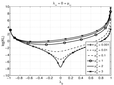
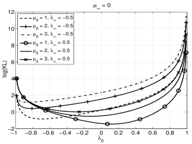
(a)	(b)
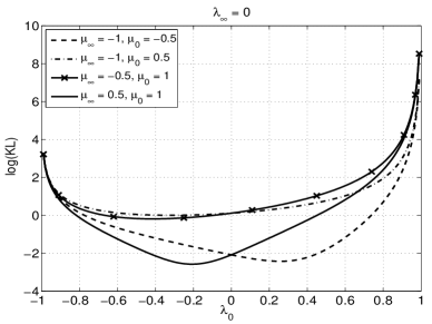
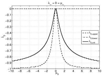
(c)	(d)
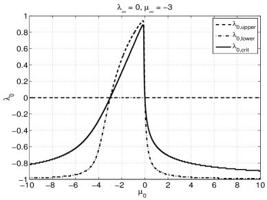
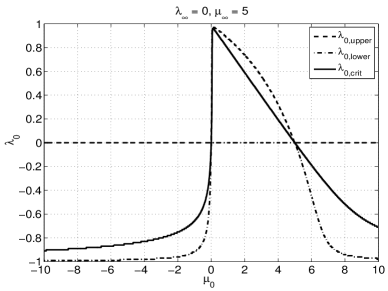
(e)	(f)

Figure 1: KL number for different sets of AR process parameters: (a) i.i.d. pre-change ($\lambda_{\infty}=0$) with $\mu_{\infty}=0$, (b) $\mu_{\infty}=0$, and (c) $\lambda_{\infty}=0$. (d)-(f) $\lambda_{0,\hskip 1.4457pt{\sf upper}}$, $\lambda_{0,\hskip 1.4457pt{\sf lower}}$ and $\lambda_{0,\hskip 1.4457pt{\sf crit}}$ as a function of $\mu_{0}$ in the i.i.d. pre-change setting ($\lambda_{\infty}=0$) for different values of $\mu_{\infty}$.

The KL number in the i.i.d. pre-change case ($\lambda_{\infty}=0$) with $\mu_{\infty}=0$ is plotted as a function of $\lambda_{0}$ for different values of $\mu_{0}$ in Fig. 1(a). Similarly, the KL number corresponding to the $\mu_{\infty}=0$ and $\lambda_{\infty}=0$ settings are plotted as a function of $\lambda_{0}$ for different combinations of parameters in Figs. 1(b) and (c), respectively. These plots clearly illustrate the existence of a certain worst-case (in the sense of detectability) post-change correlation that leads to the smallest value of $\operatorname{\mathds{I}}$ conditioned on the other model parameters. To understand this behavior of $\operatorname{\mathds{I}}$, we now study these special cases more carefully.

In the case where $\mu_{\infty}=\mu_{0}(\triangleq\mu)$, $\operatorname{\mathds{I}}$ reduces to

$$\operatorname{\mathds{I}} \triangleq\dfrac{(\lambda_{0}-\lambda_{\infty})^{2}}{2(1-\lambda_{0}^{2})}\cdot\left[1+\mu^{2}\,\left(\frac{1+\lambda_{0}}{1-\lambda_{0}}\right)\right].$$ (16)

It can be checked that

$$\dfrac{\partial\operatorname{\mathds{I}}}{\partial\lambda_{0}} \triangleq\dfrac{\lambda_{0}-\lambda_{\infty}}{(1-\lambda_{0})^{2}}\cdot\left[\mu^{2}\cdot\dfrac{1-\lambda_{\infty}}{1-\lambda_{0}}+\frac{1-\lambda_{0}\lambda_{\infty}}{(1+\lambda_{0})^{2}}\right].$$ (17)

Thus, for a fixed $\lambda_{\infty}$ and $\mu$, ${\operatorname{\mathds{I}}}$ in (16) decreases in $\lambda_{0}$ for all $\lambda_{0}<\lambda_{\infty}$ with ${\operatorname{\mathds{I}}}=0$ obtained at $\lambda_{0}=\lambda_{\infty}$. ${\operatorname{\mathds{I}}}$ then starts increasing from $0$ as $\lambda_{0}$ increases past $\lambda_{\infty}$. Specifically, a higher correlation in the post-change process increases ${\operatorname{\mathds{I}}}$ provided that both the processes are positively correlated.

When the observations are i.i.d. pre-change ($\lambda_{\infty}=0)$ with $\mu_{\infty}=0$, ${\operatorname{\mathds{I}}}$ reduces to

$$\operatorname{\mathds{I}}=\frac{1}{2(1-\lambda_{0})}\cdot\left[\frac{\lambda_{0}^{2}}{1+\lambda_{0}}+\frac{\mu_{0}^{2}}{1-\lambda_{0}}\right].$$ (18)

For a fixed $\mu_{0}$, it can be checked that

$$\frac{\partial\operatorname{\mathds{I}}}{\partial\lambda_{0}}=\frac{1}{(1-\lambda_{0})^{3}}\cdot\left[\frac{\lambda_{0}(1-\lambda_{0})}{(1+\lambda_{0})^{2}}+\mu_{0}^{2}\right].$$

From the above equation, a trivial calculation shows that ${\operatorname{\mathds{I}}}$ is globally minimized at $\lambda_{0,\hskip 1.4457pt{\sf crit}}$, defined as,

$$\lambda_{0,\hskip 1.4457pt{\sf crit}}\triangleq\frac{\sqrt{8\mu_{0}^{2}+1}-(2\mu_{0}^{2}+1)}{2(\mu_{0}^{2}-1)}.$$

Further, the KL number of the correlated process is smaller than $\mu_{0}^{2}/2$ (the KL number of the corresponding i.i.d. problem) if and only if $\lambda_{0}$ belongs to the interval $\left[\lambda_{0,\hskip 1.4457pt{\sf lower}},\hskip 1.4457pt\lambda_{0,\hskip 1.4457pt{\sf upper}}\right]$, where

$$\lambda_{0,\hskip 1.4457pt{\sf lower}}\triangleq\max\left(-1,\frac{1}{2}\cdot\left[1-\sqrt{\frac{9\mu_{0}^{2}+1}{\mu_{0}^{2}+1}}\right]\right)\hskip 3.61371pt{\rm and}\hskip 3.61371pt\lambda_{0,\hskip 1.4457pt{\sf upper}}=0.$$

It can be checked that $-1\leq\lambda_{0,\hskip 1.4457pt{\sf lower}}\leq\lambda_{0,\hskip 1.4457pt{\sf crit}}\leq\lambda_{0,\hskip 1.4457pt{\sf upper}}=0$ for all $\mu_{0}$ with both $\lambda_{0,\hskip 1.4457pt{\sf lower}}$ and $\lambda_{0,\hskip 1.4457pt{\sf crit}}$ decreasing in $\mu_{0}^{2}$. Further, we also have

$$\lambda_{0,\hskip 1.4457pt{\sf lower}}\rightarrow 0\hskip 3.61371pt{\rm and}\hskip 3.61371pt\lambda_{0,\hskip 1.4457pt{\sf crit}}\rightarrow 0 {\rm as} \mu_{0}\rightarrow 0$$

$$\lambda_{0,\hskip 1.4457pt{\sf lower}}\rightarrow-1\hskip 3.61371pt{\rm and}\hskip 3.61371pt\lambda_{0,\hskip 1.4457pt{\sf crit}}\rightarrow-1 {\rm as} \mu_{0}\rightarrow\infty.$$

See Fig. 1(d) for a plot of the three quantities as a function of $\mu_{0}$. In Figs. 1(e)-(f), these three quantities are plotted as a function of $\mu_{0}$ when $\mu_{\infty}=-3$ and $\mu_{\infty}=5$, respectively. Note that, in general, the behavior of all the three quantities is asymmetric in $\mu_{0}$.

More generally, if $\lambda_{\infty}\neq 0$, the behavior of $\lambda_{0,\hskip 1.4457pt{\sf upper}}$, $\lambda_{0,\hskip 1.4457pt{\sf lower}}$ and $\lambda_{0,\hskip 1.4457pt{\sf crit}}$ as a function of $\lambda_{\infty}$ for different $\mu_{\infty}$ and $\mu_{0}$ values is presented in Figs. 2(a)-(b). From Figs. 1(d)-(f) and Figs. 2(a)-(b), we observe that either $\lambda_{0,\hskip 1.4457pt{\sf lower}}$ or $\lambda_{0,\hskip 1.4457pt{\sf upper}}$ equals $\lambda_{\infty}$ for every case in the model parameter space. The observed trends depend on the precise relationship between $\mu_{\infty}$, $\mu_{0}$ and $0$ and can be summarized as follows:

$$\begin{array}[]{ccl}0<\mu_{0}<\mu_{\infty}\hskip 7.22743pt{\rm or}\hskip 7.22743pt\mu_{\infty}<\mu_{0}<0&\Longrightarrow&\lambda_{0,\hskip 1.4457pt{\sf lower}}=\lambda_{\infty}\\ \mu_{0}<0<\mu_{\infty}\hskip 7.22743pt{\rm or}\hskip 7.22743pt0<\mu_{\infty}<\mu_{0}\hskip 7.22743pt{\rm or}\hskip 7.22743pt\mu_{0}<\mu_{\infty}<0\hskip 7.22743pt{\rm or}\hskip 7.22743pt\mu_{\infty}<0<\mu_{0}&\Longrightarrow&\lambda_{0,\hskip 1.4457pt{\sf upper}}=\lambda_{\infty}.\end{array}$$ (21)

To summarize the above analysis, the KL number, $\operatorname{\mathds{I}}\triangleq\operatorname{\mathds{I}}(\mu_{\infty},\mu_{0},\lambda_{\infty},\lambda_{0})$, associated with the AR(1) model in (1) and given by (14), is always larger than the KL number for the basic i.i.d. problem for post-change correlation above and below certain cut-off values. In the intervening regime, the KL number is smaller than the i.i.d. problem with a worst-case $\lambda_{0}$ given by $\lambda_{0,\hskip 1.4457pt{\sf crit}}$. These trends are illustrated pictorially in Figs. 1(a)-(c).

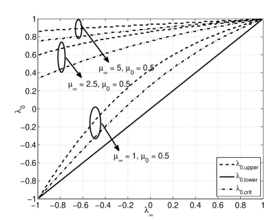
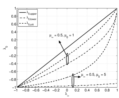
(a)	(b)

Figure 2: $\lambda_{0,\hskip 1.4457pt{\sf upper}}$, $\lambda_{0,\hskip 1.4457pt{\sf lower}}$ and $\lambda_{0,\hskip 1.4457pt{\sf crit}}$ as a function of $\lambda_{\infty}$ with different $\mu_{\infty}$ and $\mu_{0}$ values.

4 Performance Evaluation

This section is devoted to developing a numerical framework to evaluate the performance of the CUSUM chart (8)–(10) and the SR procedure (5)–(7) when applied to the AR(1) model in (1). Specifically, for each of the stopping times—either $T=\tau_{\sf cs}$ if it is the CUSUM chart, or $T=\tau_{\sf sr}$ if it is the SR procedure—the framework is “tailored” to two antagonistic performance characteristics: a) the usual “in-control” ARL to false alarm, i.e., $\operatorname{ARL}(T)$, and b) Pollak’s [15] Supremum (conditional) Average Detection Delay, i.e., $\operatorname{SADD}(T)$.

The framework here is a build-up to the one previously offered and applied in [56, 19, 20] for the i.i.d. model (with no cross-dependence in the observed data); see also, e.g., [69, 57, 58]. Accordingly, just as the prototype framework of [56, 19, 20, 69, 57, 58], our framework is also developed in two stages: we first derive a renewal integral equation for each performance metric involved, and then, as neither one of the obtained equations can be solved analytically, we supply a numerical method to do so, and carry out an analysis of the method’s accuracy. What is new in the setting considered here is that the integral equations are not one- but two-dimensional, and (therefore) the numerical method is not deterministic but rather a Monte-Carlo-type estimation technique of prescribed proportional closeness, a criterion considered, e.g., in [70, p. 339], [71, 72, 73, 74, 75].

4.1 The renewal equations

To compute the performance of the CUSUM chart (8)–(10) and that of the SR procedure (5)–(7) when applied to the AR(1) model in (1), we now derive analytically exact renewal equations on the performance characteristics of interest. To begin with, it is direct to see from (4) that $\operatorname{\Lambda}_{n}(X_{n},X_{n-1})$ is (absolutely) continuous with respect to both $X_{n}$ and $X_{n-1}$ for all $n\geq 1$. Next, given the observation series, $\{X_{n}\}_{n\geq 0}$, consider the generic detection procedure associated with the generic stopping time

$$T(x_{0},y_{0},A) \triangleq\inf\big{\{}n\geq 1\colon Y_{n}\geq A\big{\}},\;y_{0}\geq 0,\;x_{0}\in\mathbb{R},\;A>0,$$ (22)

whose decision-making is based off the generic detection statistic $\{Y_{n}\}_{n\geq 0}$ defined as

$$Y_{n} =\Psi(Y_{n-1})\operatorname{\Lambda}_{n}(X_{n-1},X_{n})\;\text{for}\;n=1,2,\ldots\;\text{with}\;Y_{0}=y_{0}\geq 0\;\text{and}\;X_{0}=x_{0}\in\mathbb{R},$$

where $\Psi(z)$ is a (sufficiently) smooth non-negative-valued function defined (at least) for $z\geq 0$, and $y_{0}\geq 0$ and $x_{0}\in\mathbb{R}$ are given constants; the assumptions that $\Psi(z)\geq 0$ for $z\geq 0$ and that $y_{0}\geq 0$ are necessary to ensure that $\{Y_{n}\}_{n\geq 0}$ is almost surely non-negative under any probability measure, so that the two-dimensional (homogeneous) Markov process, $\{(Y_{n},X_{n})\}_{n\geq 0}$, is restricted to the half-plane $[0,\infty)\times\mathbb{R}$.

Now note that since the choice of $\Psi(z)$ is flexible, the generic stopping time $T(x,y,A)$ can be seen to describe a rather large class of LR-based detection procedures; in particular, if $\Psi(z)=1+z$, then $\{Y_{n}\}_{n\geq 0}$ and the SR detection statistic, $\{R_{n}\}_{n\geq 0}$, are identical, and therefore, for this choice of $\Psi(z)$ the generic stopping time $T(x,y,A)$ and that associated with the SR procedure coincide. Hence, the SR procedure is a special case of $T(x,y,A)$, as is the CUSUM chart; indeed, if $\Psi(z)=\max\{1,z\}$, then $\{Y_{n}\}_{n\geq 0}$ is the CUSUM detection statistic, $\{V_{n}\}_{n\geq 0}$, and therefore, in this case the generic stopping time $T(x,y,A)$ is no different from that associated with the CUSUM chart. This flexibility of the generic stopping time $T(x,y,A)$ can be used to study simultaneously the performance of not only the CUSUM chart or the SR procedure, but also of a far larger number of other procedures (e.g., EWMA procedure).

Let $\mathbb{P}_{d}(Y_{n}\leq y_{2},X_{n}\leq x_{2}|Y_{n-1}=y_{1},X_{n-1}=x_{1})$, $d=\{0,\infty\}$, denote the transition probability function to describe the evolution (in time, $n$) of the two-dimensional (homogeneous) Markov process $\{(Y_{n},X_{n})\}_{n\geq 0}$ under probability measure $\mathbb{P}_{d}$, $d=\{0,\infty\}$; note that $\mathbb{P}_{d}(Y_{n}\leq y_{2},X_{n}\leq x_{2}|Y_{n-1}=y_{1},X_{n-1}=x_{1})$, $d=\{0,\infty\}$, is independent of $n$. Let

$$K_{d}(y_{2},x_{2}|y_{1},x_{1}) \triangleq\dfrac{\partial^{2}}{\partial y_{2}\partial x_{2}}\mathbb{P}_{d}(Y_{n}\leq y_{2},X_{n}\leq x_{2}|Y_{n-1}=y_{1},X_{n-1}=x_{1}),$$ (23)

$d=\{0,\infty\}$, be the respective transition probability density kernel; it is clear that $K_{d}(y_{2},x_{2}|y_{1},x_{1})$, $d=\{0,\infty\}$, is independent of $n$ as well. A straightforward calculation shows that

$$\mathbb{P}_{d}(Y_{n}\leq y_{2},X_{n}\leq x_{2}|Y_{n-1}=y_{1},X_{n-1}=x_{1})$$

$$=\left\{\begin{array}[]{cc}\Phi(\min\{x_{2},\xi(x_{1},y_{1},y_{2})\}-\mu_{d}-\lambda_{d}x_{1}),&{\rm if}\hskip 3.61371pt\mu_{0}-\mu_{\infty}+x_{1}(\lambda_{0}-\lambda_{\infty})\geq 0\\ \Phi(x_{2}-\mu_{d}-\lambda_{d}x_{1})-\Phi(\xi(x_{1},y_{1},y_{2})-\mu_{d}-\lambda_{d}x_{1}),&{\rm if}\hskip 3.61371pt\mu_{0}-\mu_{\infty}+x_{1}(\lambda_{0}-\lambda_{\infty})<0,\end{array}\right.$$

where

$$\xi(x_{1},y_{1},y_{2}) \triangleq\dfrac{1}{\mu_{0}-\mu_{\infty}+x_{1}(\lambda_{0}-\lambda_{\infty})}\log\left(\dfrac{y_{2}}{\Psi(y_{1})}\right)+\dfrac{\mu_{0}+\mu_{\infty}+x_{1}(\lambda_{0}+\lambda_{\infty})}{2},$$

and

$$\Phi(x) \triangleq\dfrac{1}{\sqrt{2\pi}}\int_{-\infty}^{x}e^{-\tfrac{t^{2}}{2}}dt,$$

i.e., the standard Gaussian cdf.

We are now in a position to derive the first renewal equation of interest, viz., that on the first moment of $T(x_{0},y_{0},A)$ under measure $\mathbb{P}_{\infty}$, i.e., for the ARL to false alarm of the generic stopping time $T(x_{0},y_{0},A)$. Specifically, for notational brevity, denote $\ell(x,y,A)\triangleq\operatorname{\mathbb{E}}_{\infty}[T(x,y,A)]$. By conditioning on the first observation, $X_{1}$, and using a routine renewal argument akin to that made in [20] we obtain

$$\ell(x_{1},y_{1},A) =1+\int_{-\infty}^{\infty}\int_{0}^{A}K_{\infty}(y_{2},x_{2}|y_{1},x_{1})\,\ell(x_{2},y_{2},A)\,dy_{2}\,dx_{2}.$$ (24)

The double integral in the right-hand side of this equation cannot be separated, since $Y_{n}$ and $X_{n}$ are correlated for all $n\geq 1$. However, it is because $Y_{n}$ and $X_{n}$ are correlated for all $n\geq 1$, the double integral is effectively a single integral, and is taken along the curve given by the points $(y_{2},x_{2})$ for which $K_{\infty}(y_{2},x_{2}|y_{1},x_{1})\neq 0$. These points satisfy the equation $u(x_{1},y_{1},y_{2})=x_{2}$, or written explicitly

$$\dfrac{1}{\mu_{0}-\mu_{\infty}+x_{1}(\lambda_{0}-\lambda_{\infty})}\log\left(\dfrac{y_{2}}{\Psi(y_{1})}\right)+\dfrac{\mu_{0}+\mu_{\infty}+x_{1}(\lambda_{0}+\lambda_{\infty})}{2} =x_{2},$$

and for all other values of $(x_{1},y_{1})$ and $(x_{2},y_{2})$ the integral is zero, and $\ell(x_{1},y_{1},A)=1$ irrespective of $A>0$.

Thus, the double integral in the right-hand side of (24) is to be understood in the Riemann–Stieltjes sense with the measure of integration being $\mathbb{P}_{\infty}(Y_{n}\leq y_{2},X_{n}\leq x_{2}|Y_{n-1}=y_{1},X_{n-1}=x_{1})$. Since the latter is a two-dimensional cdf, it is clearly a function of bounded variation, and therefore the existence of the integral is justified.

Next, introduce $\delta_{0}(x,y,A)\triangleq\operatorname{\mathbb{E}}_{0}[T(x,y,A)]$, and observe that

$$\delta_{0}(x_{1},y_{1},A) =1+\int_{-\infty}^{\infty}\int_{0}^{A}K_{0}(y_{2},x_{2}|y_{1},x_{1})\,\delta_{0}(x_{2},y_{2},A)\,dy_{2}\,dx_{2},$$ (25)

which is an exact “copy” of equation (24) except that $K_{\infty}(y_{2},x_{2}|y_{1},x_{1})$ is replaced with $K_{0}(y_{2},x_{2}|y_{1},x_{1})$. For $k\geq 1$, since $\{R_{n}^{r=x}\}_{n\geq 0}$ is Markovian, one can establish the recursion

$$\delta_{k+1}(x_{1},y_{1},A) =\int_{-\infty}^{\infty}\int_{0}^{A}{K}_{\infty}(y_{2},x_{2}|y_{1},x_{1})\,\delta_{k}(x_{2},y_{2},A)\,dy_{2}\,dx_{2},\;k\geq 0,$$ (26)

with $\delta_{0}(x,y,A)$ first found from equation (25); cf. [20]. Using this recursion one can generate the entire functional sequence $\{\delta_{k}(x,y,A)\}_{k\geq 0}$ by repetitive application of the linear integral operator

$$\mathcal{K}_{\infty}\circ u \triangleq[\mathcal{K}_{\infty}\circ u](x_{1},y_{1})\triangleq\int_{0}^{A}{K}_{\infty}(y_{2},x_{2}|y_{1},x_{1})\,u(x_{2},y_{2})\,dy_{2}\,dx_{2},$$

where $u(x,y)$ is assumed to be sufficiently smooth inside the strip $\mathbb{R}\times[0,A]$. Temporarily deferring formal discussion of this operator’s properties, note that using this operator notation, recursion (26) can be rewritten as $\delta_{k+1}=\mathcal{K}_{\infty}\circ\delta_{k}$, $k\geq 0$, or equivalently, as $\delta_{k}=\mathcal{K}_{\infty}^{k}\circ\delta_{0}$, $k\geq 0$, where

$$\mathcal{K}_{\infty}^{k}\circ u \triangleq\underbrace{\mathcal{K}_{\infty}\circ\cdots\circ\mathcal{K}_{\infty}}_{\text{$k$ times}}\circ\,u\;\text{for}\;k\geq 1,$$

and $\mathcal{K}_{\infty}^{0}$ is the identity operator from now on denoted as $\mathbb{I}$, i.e., $\mathcal{K}_{\infty}^{0}\circ u=\mathbb{Id}\circ u\triangleq u$. Similarly, in the operator form, equation (24) can be rewritten as $\ell=1+\mathcal{K}_{\infty}\circ\ell$, and equation (25) can be rewritten as $\delta_{0}=1+\mathcal{K}_{0}\circ\delta_{0}$.

Lemma 1.

For the generic detection procedure $T(x_{0},0,A)$ given by (22) it is true that

$$\operatorname{SADD}(T(x_{0},0,A)) \triangleq\sup_{0\leq k<\infty}\operatorname{ADD}_{k}(T(x_{0},0,A))$$

$$=\operatorname{ADD}_{0}(T(x_{0},0,A))\triangleq\operatorname{\mathbb{E}}_{0}[T(x_{0},0,A)].$$

Equations (24) and (25) provide a “complete package” to compute any of the desired performance characteristics of the CUSUM chart and those of the SR procedure. The question to be considered next is to compute these characteristics in practice.

4.2 The numerical solution and its accuracy

The renewal equations established in the preceding subsection on the performance metrics of interest are (two-dimensional) Fredholm (linear) integral equations of the second kind. Such equations rarely permit an analytical, closed-form solution, even in a single dimension. Hence, a numerical method is in order, and it is the aim of this subsection to propose one.

The branch of numerical analysis concerned with the design and analysis of numerical schemes to solve Fredholm integral equations of the second kind has plenty of powerful methods for efficient solution of these equations in one dimension. However, even then the dimension is two, things get much more complicated. We propose to consider a Markov Chain Monte-Carlo (MCMC) technique.

We start with an observation that although the integral involved in the equation of interest is a double integral, it can actually be reduced to a single equation, as $X_{n}$ and $R_{n}$ are dependent on one another. Specifically, this single integral is along the curve described in the $(X_{n},R_{n})$ space by the relation $R_{n}=(1+R_{n-1})\operatorname{\Lambda}_{n}$, where both $X_{n-1}$ and $R_{n-1}$ are assumed fixed. Let us therefore deal with a single-dimensional equivalent of the equation of interest:

$$u(x) =1+\int{K}(x,y)\,u(y)\,dy,$$ (27)

where $\mathcal{K}(x,y)\geq 0$, $\forall(x,y)\in\mathbb{R}^{2}$, is the respective transition probability density for the appropriate Markov chain.

It is known (and can be easily shown) that the solution to this equation admits the following Neumann series:

$$\begin{aligned} u(z_{0})&=1+\int_{[0,A]}{K}(z_{0},z_{1})\,dz_{1}+\int_{\otimes_{i=1}^{2}[0,A]}{K}(z_{0},z_{1})\,{K}(z_{1},z_{2})\,dz_{1}\,dz_{2}\\ &\qquad\qquad\qquad+\int_{\otimes_{i=1}^{3}[0,A]}{K}(z_{0},z_{1})\,{K}(z_{1},z_{2})\,{K}(z_{2},z_{3})\,dz_{1}\,dz_{2}\,dz_{3}+\ldots\\ &=1+\sum_{k=1}^{\infty}\int_{\otimes_{i=1}^{k}[0,A]}\left(\prod_{j=1}^{k}{K}(z_{j-1},z_{j})\right)dz_{1}\,dz_{1}\ldots dz_{k},\end{aligned}$$

where $\otimes$ denotes the usual direct product (as applied to sets).

We first note that equation (27) can be solved either at a particular (single) point, or over a particular interval. We are interested in the former, with the point being zero, i.e., when the detection statistic has no headstart. For the actual solution method to obtain $u(0)\triangleq\operatorname{\mathbb{E}}[T]$, one option would be to use a deterministic numerical scheme to “linearize” the integral in the right-hand side of (27), and then, to ensure the linearization is “optimal”, reduce the integral equation to a system of linear equations for a vector approximating the unknown function [76]. The problem with this approach is that the integral is actually two-dimensional, and is over an unbounded region. As a result, it is difficult to “chop up” the region of integration to form a partition of reasonable size. To overcome this problem, we suggest to consider a Monte Carlo technique.

The idea of the basic Monte Carlo approach to evaluate $u(0)\triangleq\operatorname{\mathbb{E}}[T]$ is to compute it statistically, i.e., to—in one way or another—estimate it based on a (somehow) generated sample, $\{T_{j}\}_{1\leq j\leq N}$, of $N\geq 1$ independent instantiations of the (same) stopping time $T$. Specifically, let $\widehat{\operatorname{\mathbb{E}}[T]}$ denote an estimator of $\operatorname{\mathbb{E}}[T]$. The standard choice for $\widehat{\operatorname{\mathbb{E}}[T]}$ is to use the sample mean

$$\bar{T}_{N} \triangleq\dfrac{1}{N}\sum_{j=1}^{N}T_{j},$$

which is well-justified since the sample mean is unbiased (for any $N\geq 1$), and, due to the (strong) Law of Large Numbers, is also asymptotically (as $N\to\infty$) consistent.

While it is not a problem to simulate as many independent instantiations of $T$ as necessary (even if $N$ is $10^{6}$ or higher), the question of proximity of the respective estimate $\widehat{\operatorname{\mathbb{E}}[T]}\triangleq\bar{T}_{N}$ to the actual true (but unknown) value of $\operatorname{\mathbb{E}}[T]$ is to be addressed with care. To that end, the standard solution is to construct a $(1-\epsilon)\,\%$-confidence interval, $\epsilon\in(0,1)$, of a prescribed width, $w>0$. Specifically, let $\sigma_{T}$ denote the standard deviation of $T$, i.e., $\sigma_{T}\triangleq\sqrt{\operatorname{Var}[T]}$. If $\sigma_{T}$ is known, then from the Central Limit Theorem (CLT) we immediately have

$$\sqrt{N}\,\dfrac{\bar{T}_{N}-\operatorname{\mathbb{E}}[T]}{\sigma_{T}}\underset{N\to\infty}{\overset{d}{\longrightarrow}}\mathcal{N}(0,1),$$

and therefore, to ensure that

$$\mathbb{P}\left(\dfrac{|\bar{T}_{N}-\operatorname{\mathbb{E}}[T]|}{\sigma_{T}}\leq w\right) \geq 1-\epsilon,$$

it suffices to take the sample size $N$ as

$$N \geq\left\lfloor 2z_{\epsilon/2}\frac{\sigma_{T}}{w}\right\rfloor+1,$$

where $\lfloor x\rfloor$ is the floor function, and $z_{\epsilon/2}$ is the $\epsilon/2$-th percentile of the standard Gaussian distribution. Rephrasing this, for this choice of $N$, with probability of at least $1-\epsilon\in(0,1)$, the unknown true mean $\operatorname{\mathbb{E}}[T]$ of the stopping time $T$ will be contained in the interval $(\bar{T}_{N}-w,\bar{T}_{N}+w)$, i.e., it will be true that $\mathbb{P}\left(\bar{T}_{N}-w\leq\operatorname{\mathbb{E}}[T]\leq\bar{T}_{N}+w\right)\geq 1-\epsilon$.

As may be seen, the problem with this approach is that the standard deviation, $\sigma_{T}$, is not known. One could, of course, estimate it, and then build a confidence interval off the estimated value, $\hat{\sigma}_{T}$. The issue with this idea, however, is that the distribution of $(\bar{T}_{N}-\operatorname{\mathbb{E}}[T])/\hat{\sigma}_{T}$ may fail to be normal, even asymptotically, as $N\to\infty$. A more elegant way out of this is to note that if the detection statistic’s headstart is zero, which is the case in this work, then $\sigma_{T}\leq\operatorname{\mathbb{E}}[T]$. With formal proof of this inequality temporarily deferred, let us illustrate what it can lead to. Since $\sigma_{T}\leq\operatorname{\mathbb{E}}[T]$ and $\operatorname{\mathbb{E}}[T]>0$ (in fact $\operatorname{\mathbb{E}}[T]\geq 1$), the event $\big{\{}|\bar{T}_{N}-\operatorname{\mathbb{E}}[T]|\leq w\operatorname{\mathbb{E}}[T]\big{\}}$ is contained in the event $\big{\{}|\bar{T}_{N}-\operatorname{\mathbb{E}}[T]|\leq w\sigma_{T}\big{\}}$, and therefore

$$\mathbb{P}\left(\dfrac{|\bar{T}_{N}-\operatorname{\mathbb{E}}[T]|}{\operatorname{\mathbb{E}}[T]}<w\right) \geq\mathbb{P}\left(\dfrac{|\bar{T}_{N}-\operatorname{\mathbb{E}}[T]|}{\sigma_{T}}<w\right),$$

so that confidence bounds for the relative error, $|\bar{T}_{N}-\operatorname{\mathbb{E}}[T]|/\operatorname{\mathbb{E}}[T]$, are readily available; in this case $w$ is measured in percentages. This criterion is known as prescribed proportional closeness [70, p. 339], [71, 72, 73, 74, 75].

We now prove the claim made earlier that $\sigma_{T}\leq\operatorname{\mathbb{E}}[T]$ when the detection statistic has no headstart. Let $\mathfrak{M}_{k}(x,A)\triangleq\operatorname{\mathbb{E}}[T^{k}(x,A)]$ with $k\in\mathbb{N}$, i.e., $\mathfrak{M}_{k}(x,A)$ is the $k$-th moment of the stopping time $T(x,A)$; in particular, $\mathfrak{M}_{1}(x,A)\triangleq\operatorname{\mathbb{E}}[T(x,A)]$. We will need the following two lemmas.

Lemma 2.

$\mathfrak{M}_{1}(x,A)\leq\mathfrak{M}_{1}(0,A)$ for any given $A>0$ and $x\geq 0$.

Proof.

The sought-after inequality $\mathfrak{M}_{1}(x,A)\leq\mathfrak{M}_{1}(0,A)$ is merely the statement that, on average, the higher the headstart of the detection statistic behind the stopping time $T(x,A)$, the sooner (on average) the respective detection procedure is to terminate. That is, the closer the detection statistic is initially to the detection threshold, $A>0$, the sooner (on average) it is to reach the threshold, and therefore, the sooner (on average) the detection procedure is to stop. ∎

Lemma 3.

$\big{[}(\mathbb{I}-\mathcal{K})^{-1}\circ\mathfrak{M}_{1}\big{]}(x,A)\leq\mathfrak{M}_{1}(0,A)\,\mathfrak{M}_{1}(x,A)$ for any given $A>0$ and $x\geq 0$.

Proof.

The desired result is a direct consequence of Lemma 2, i.e., the inequality $\mathfrak{M}_{1}(x,A)\leq\mathfrak{M}_{1}(0,A)$, $\forall x\geq 0$, applied to upperbound each summand in the respective Neumann expansion for $\big{[}(\mathbb{I}-\mathcal{K})^{-1}\circ\mathfrak{M}_{1}\big{]}(x,A)$. ∎

With Lemma 2 and Lemma 3 in mind, it is easy to see that $\big{[}(\mathbb{I}-\mathcal{K})^{-1}\circ\mathfrak{M}_{1}\big{]}(x,A)\leq\mathfrak{M}_{1}^{2}(0,A)$. As shown in [57], the second moment, $\mathfrak{M}_{2}(x,A)\triangleq\operatorname{\mathbb{E}}[T^{2}(x,A)]$, of the generic stopping time, $T(x,A)$, is governed by the integral equation $\mathfrak{M}_{2}=2\mathfrak{M}_{1}-1+\mathcal{K}\circ\mathfrak{M}_{2}$, where $\mathfrak{M}_{1}(x,A)\triangleq\operatorname{\mathbb{E}}[T(x,A)]$. The operator solution to this equation is of the form $\mathfrak{M}_{2}=2(\mathbb{I}-\mathcal{K})^{-1}\circ\mathfrak{M}_{1}-\mathfrak{M}_{1}$. Finally, since $\operatorname{Var}[T]=\mathfrak{M}_{2}-\mathfrak{M}_{1}^{2}$, and $\mathcal{K}\circ\mathfrak{M}_{1}=\mathfrak{M}_{1}-1\leq\mathfrak{M}_{1}$, we obtain

$$\mathfrak{M}_{2}(x,A) =2\big{[}(\mathbb{I}-\mathcal{K})^{-1}\circ\mathfrak{M}_{1}\big{]}(x,A)-\mathfrak{M}_{1}(x,A)$$

$$\leq 2\mathfrak{M}_{1}^{2}(0,A)-\mathfrak{M}_{1}(x,A)$$

$$\leq 2\mathfrak{M}_{1}^{2}(0,A).$$

Therefore, $\mathfrak{M}_{2}(0,A)\leq 2\mathfrak{M}_{1}^{2}(0,A)$, and we have

$$\sigma_{T}^{2}\triangleq\operatorname{Var}[T(0,A)] \triangleq\mathfrak{M}_{2}(0,A)-\mathfrak{M}_{1}^{2}(0,A)$$

$$\leq\mathfrak{M}_{1}^{2}(0,A),$$

which is to say that $\sigma_{T}\leq\operatorname{\mathbb{E}}[T]$, provided the detection statistic starts off zero (no headstart). We stress that the assumption of no headstart is a critical one, and when the detection statistic does have a (non-zero) headstart, the inequality $\sigma_{T}\leq\operatorname{\mathbb{E}}[T]$ may fail to hold.

We conclude this subsection with a remark on how to reduce the variance of the sample mean $\bar{T}_{N}$. The idea is that since the first two terms in the Neumann series are always computable exactly, as such there is no need to estimate either one of them. Hence, instead of sampling the trajectories from $\mathcal{K}(x,y)$ assuming the starting point is 0, one may start each trajectory off a random point, sampled from $\mathcal{K}(x,y)$, but restricted to the interval $[0,A]$.

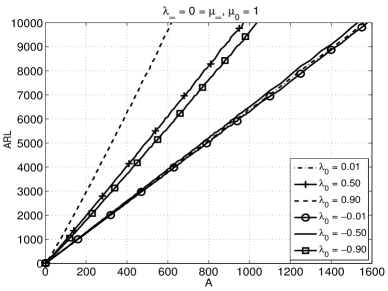
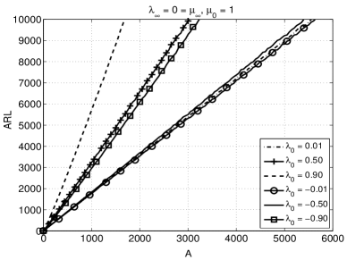
(a)	(b)
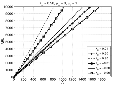
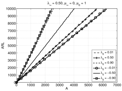
(c)	(d)
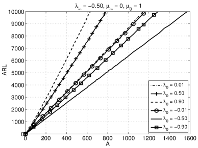
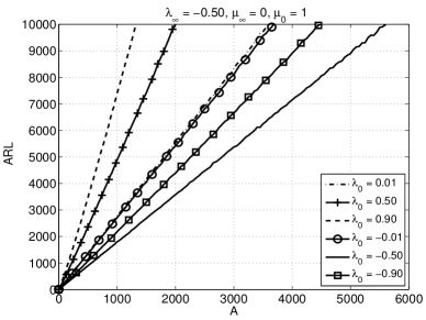
(e)	(f)

i

Figure 3: $\operatorname{ARL}$ as a function of threshold $A$ for the (a) CUSUM chart and (b) SR procedure in the i.i.d. pre-change setting with $\mu_{\infty}=0$. $\operatorname{ARL}$ vs. $A$ for the CUSUM chart and SR procedure in the case where (c)-(d) $\lambda_{\infty}=0.50$ and (e)-(f) $\lambda_{\infty}=-0.50$ for different $\lambda_{0}$ values.

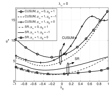
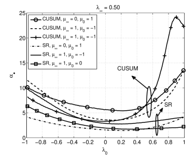
(a)	(b)
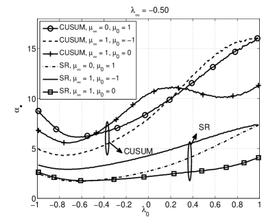
(c)

Figure 4: Estimates of $\alpha_{\sf cs}$ and $\alpha_{\sf sr}$ as a function of $\lambda_{0}$ under three different settings for pre-change and post-change means.

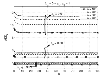
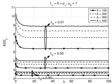
(a)	(b)
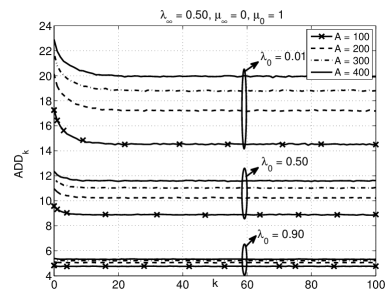
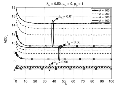
(c)	(d)
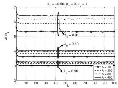
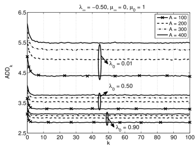
(e)	(f)

Figure 5: $\operatorname{ADD}_{k}$ as a function of $k$ in the i.i.d. pre-change setting with $\mu_{\infty}=0$ for the (a) CUSUM chart and (b) SR procedure. $\operatorname{ADD}_{k}$ vs. $k$ for the CUSUM chart and SR procedure in the case where (c)-(d) $\lambda_{\infty}=0.50$ and (e)-(f) $\lambda_{\infty}=-0.50$.

5 Numerical Studies

We now apply the numerical techniques illustrated in the preceding section to compute ARL and SADD and perform a comparative analysis of the CUSUM chart and SR procedure. But before this, we need to design the procedures carefully.

5.1 Designing the CUSUM chart and SR procedure

The design of the CUSUM chart and the SR procedure requires an understanding of how the threshold $A$ should be set (as a function of $\gamma$) to ensure that the $\operatorname{ARL}$ with either procedure is at least $\gamma$. For this, we study the $\operatorname{ARL}$ behavior of both procedures numerically as a function of the threshold $A$. In the i.i.d. pre-change setting with $\mu_{\infty}=0$ and $\mu_{0}=1$, Figs. 3(a) and (b) plot $\operatorname{ARL}$ for the CUSUM chart and the SR procedure, respectively, for different values of $A$ and $\lambda_{0}$. In Figs. 3(c)-(d), $\operatorname{ARL}$ vs. $A$ is plotted for the CUSUM chart and SR procedure with $\lambda_{\infty}=0.50$ and several $\lambda_{0}$ values. Similarly, in Figs. 3(e)-(f), $\operatorname{ARL}$ vs. $A$ is plotted for the two procedures with $\lambda_{\infty}=-0.50$ and several $\lambda_{0}$ values. The robust linear dependence in our studies (across different parameter values) suggests the following empirical relationship (as $A\rightarrow\infty$):

$$\operatorname{ARL}(\tau_{\sf cs})=\alpha_{\sf cs}\cdot A+\beta_{\sf cs}, \operatorname{ARL}(\tau_{\sf sr})=\alpha_{\sf sr}\cdot A+\beta_{\sf sr},$$ (28)

for some constants $\{\alpha_{\bullet}\}$ and $\{\beta_{\bullet}\}$ depending only on the model parameters. To further understand the behavior of $\alpha_{\sf cs}$ and $\alpha_{\sf sr}$ as a function of the model parameters, in Figs. 4(a)-(c), we plot estimates of these quantities as a function of $\lambda_{0}$ in three settings where $\lambda_{\infty}=0$, $\lambda_{\infty}=0.50$ and $\lambda_{\infty}=-0.50$, each with: i) $\mu_{\infty}=0$ and $\mu_{0}=1$, ii) $\mu_{\infty}=1$ and $\mu_{0}=-1$, and iii) $\mu_{\infty}=1$ and $\mu_{0}=0$.

Noting that $\operatorname{SADD}$ is the supremum of the conditional average detection delay ($\operatorname{ADD}_{k}$), we are interested in the choice of $k$ that maximizes $\operatorname{ADD}_{k}$. In the $\lambda_{\infty}=0=\lambda_{0}$ case, it is well-understood that this maximum occurs at $k=0$. However, generalizing this result to the AR setting seems difficult. Thus, we pursue a numerical approach in understanding this problem. In Figs. 5(a) and (b), we plot the behavior of $\operatorname{ADD}_{k}$ as a function of $k$ for the CUSUM chart and the SR procedure, respectively, for different $A$ and $\lambda_{0}$ values. The same trend is plotted in Figs. 5(c)-(d) and (e)-(f) for the CUSUM chart and SR procedure in the $\lambda_{\infty}=0.50$ and $\lambda_{\infty}=-0.50$ settings, respectively. In all the cases considered, the maximum of $\operatorname{ADD}_{k}$ occurs at $k=0$ thus suggesting that $\operatorname{SADD}=\operatorname{ADD}_{0}$ in the AR setting also. This fact is critical since Sec. 4 allows us to compute $\operatorname{ADD}_{0}(T)=\operatorname{\mathbb{E}}_{0}(T)$.

Further, from these studies, we also observe that an increase in $A$ leads to an increased $\operatorname{ADD}_{k}$ for all $k$, and the same threshold results in a higher $\operatorname{ADD}_{k}$ for the CUSUM chart relative to the SR procedure — both of which are not surprising conclusions. Also, note that for both procedures, $\operatorname{ADD}_{k}$ converges to a steady-state value ($\operatorname{ADD}_{\infty}$) quickly. $\operatorname{ADD}_{\infty}$ can be treated as the average delay in detecting a change upon repeated trials of the monitoring process. It can also be seen from Table 1 that the SR procedure is more sensitive to the change-point than the CUSUM chart as captured by a larger value for the metric $\operatorname{ADD}_{0}-\operatorname{ADD}_{\infty}$. Further, note that $\operatorname{ADD}_{0}-\operatorname{ADD}_{\infty}$ decreases as $A$ increases confirming the intuition that in the large $A$ regime (and thus large $\operatorname{ARL}$ regime from (28)), $\operatorname{ADD}_{k}$ is essentially independent of $k$.

Table 1: $\operatorname{ADD}_{0}$ and $\operatorname{ADD}_{\infty}$ for different choices of $A$, $\lambda_{\infty}$ and $\lambda_{0}$ with the CUSUM chart and the SR procedure.

		CUSUM			SR
	$A$	$\operatorname{ADD}_{0}$	$\operatorname{ADD}_{\infty}$	$\operatorname{ADD}_{0}-\operatorname{ADD}_{\infty}$	$\operatorname{ADD}_{0}$	$\operatorname{ADD}_{\infty}$	$\operatorname{ADD}_{0}-\operatorname{ADD}_{\infty}$
		$\lambda_{\infty}=0$
$\lambda_{0}=0.01$	$100$	$9.4794$	$8.7804$	$0.6990$	$7.7031$	$6.3756$	$1.3275$
	$200$	$10.8089$	$10.1006$	$0.7083$	$9.0141$	$7.6100$	$1.4041$
	$300$	$11.6191$	$10.8822$	$0.7369$	$9.8014$	$8.3579$	$1.4435$
	$400$	$12.1713$	$11.4335$	$0.7378$	$10.3568$	$8.8858$	$1.4710$
$\lambda_{0}=0.50$	$100$	$5.0596$	$4.8889$	$0.1707$	$4.6441$	$4.1965$	$0.4476$
	$200$	$5.4508$	$5.2807$	$0.1701$	$5.0438$	$4.6122$	$0.4316$
	$300$	$5.6700$	$5.5059$	$0.1641$	$5.2674$	$4.8460$	$0.4214$
	$400$	$5.8421$	$5.6598$	$0.1823$	$5.4434$	$5.0101$	$0.4333$
$\lambda_{0}=0.90$	$100$	$3.7302$	$3.6574$	$0.0728$	$3.5688$	$3.3758$	$0.1930$
	$200$	$3.8730$	$3.8218$	$0.0512$	$3.7294$	$3.5667$	$0.1627$
	$300$	$3.9778$	$3.9136$	$0.0642$	$3.8311$	$3.6697$	$0.1614$
	$400$	$4.0328$	$3.9745$	$0.0583$	$3.9018$	$3.7407$	$0.1611$
		$\lambda_{\infty}=-0.50$
$\lambda_{0}=0.01$	$100$	$5.6261$	$5.3293$	$0.2968$	$5.0340$	$4.4005$	$0.6335$
	$200$	$6.1553$	$5.8750$	$0.2803$	$5.5918$	$4.9433$	$0.6485$
	$300$	$6.4911$	$6.1949$	$0.2962$	$5.9061$	$5.2635$	$0.6426$
	$400$	$6.7129$	$6.4242$	$0.2887$	$6.1317$	$5.4905$	$0.6412$
$\lambda_{0}=0.50$	$100$	$3.8513$	$3.6362$	$0.2151$	$3.6449$	$3.3084$	$0.3365$
	$200$	$4.0576$	$3.8497$	$0.2079$	$3.8682$	$3.5411$	$0.3271$
	$300$	$4.1810$	$3.9722$	$0.2088$	$3.9885$	$3.6696$	$0.3189$
	$400$	$4.2681$	$4.0559$	$0.2122$	$4.0818$	$3.7593$	$0.3225$
$\lambda_{0}=0.90$	$100$	$3.2341$	$3.0222$	$0.2119$	$3.1334$	$2.8556$	$0.2778$
	$200$	$3.3550$	$3.1547$	$0.2003$	$3.2529$	$3.0027$	$0.2502$
	$300$	$3.4152$	$3.2281$	$0.1871$	$3.3089$	$3.0838$	$0.2251$
	$400$	$3.4542$	$3.2747$	$0.1795$	$3.3666$	$3.1348$	$0.2318$
		$\lambda_{\infty}=0.50$
$\lambda_{0}=0.01$	$100$	$17.2517$	$14.5254$	$2.7263$	$12.5621$	$9.3600$	$3.2021$
	$200$	$20.1402$	$17.2179$	$2.9223$	$15.2273$	$11.8155$	$3.4118$
	$300$	$21.8208$	$18.8028$	$3.0180$	$16.8002$	$13.3295$	$3.4707$
	$400$	$22.9024$	$19.9526$	$2.9498$	$17.9379$	$14.4156$	$3.5223$
$\lambda_{0}=0.50$	$100$	$9.5787$	$8.8826$	$0.6961$	$7.7808$	$6.4275$	$1.3533$
	$200$	$10.9615$	$10.2309$	$0.7306$	$9.1228$	$7.6872$	$1.4356$
	$300$	$11.8190$	$11.0263$	$0.7927$	$9.9153$	$8.4447$	$1.4706$
	$400$	$12.3540$	$11.5900$	$0.7640$	$10.5127$	$8.9938$	$1.5189$
$\lambda_{0}=0.90$	$100$	$4.8245$	$4.7586$	$0.0659$	$4.4862$	$4.2058$	$0.2804$
	$200$	$5.1108$	$5.0501$	$0.0607$	$4.8206$	$4.5406$	$0.2800$
	$300$	$5.2656$	$5.2123$	$0.0533$	$4.9900$	$4.7238$	$0.2662$
	$400$	$5.3880$	$5.3240$	$0.0640$	$5.1271$	$4.8481$	$0.2790$

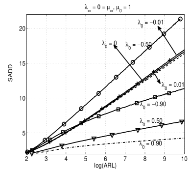
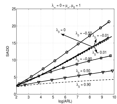
(a)	(b)
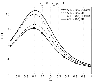
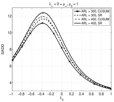
(c)	(d)

Figure 6: Performance of (a) CUSUM chart and (b) SR procedure for the i.i.d. pre-change setting for different values of $\lambda_{0}$ with $\mu_{0}=1$. (c)-(d) $\operatorname{SADD}$ as a function of $\lambda_{0}$ for the CUSUM chart and SR procedure for different $\operatorname{ARL}$ values.

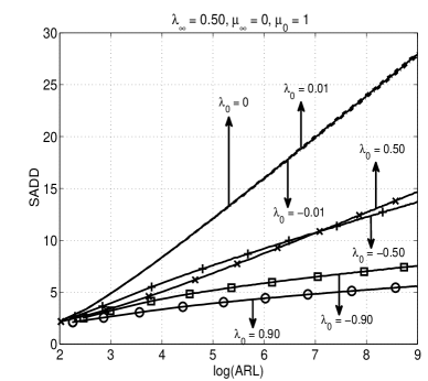
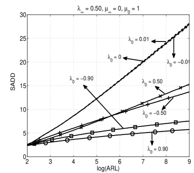
(a)	(b)
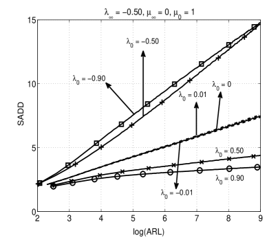
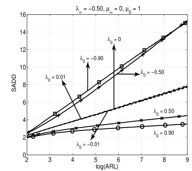
(c)	(d)

Figure 7: Performance of CUSUM chart and SR procedure (a)-(b) with $\lambda_{\infty}=0.50$ and (c)-(d) with $\lambda_{\infty}=-0.50$ for different values of $\lambda_{0}$ and $\mu_{0}=1$.

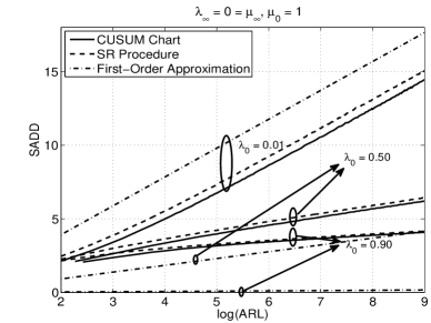
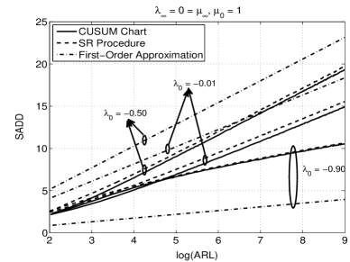
(a)	(b)
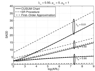
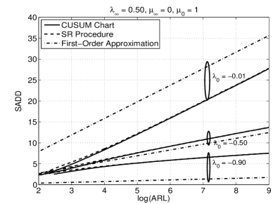
(c)	(d)
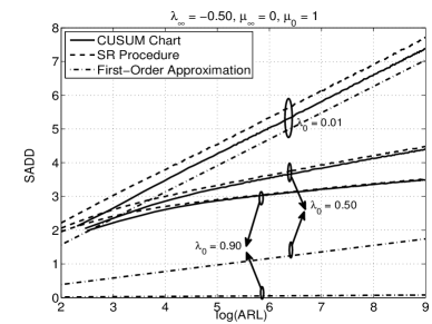
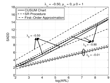
(e)	(f)

Figure 8: CUSUM chart and SR procedure performance along with the first-order approximation from (29) for the i.i.d. pre-change setting with $\mu_{\infty}=0$ for (a) select positive $\lambda_{0}$ values and (b) select negative $\lambda_{0}$ values. Similar plots are provided for the case where (c)-(d) $\lambda_{\infty}=0.50$ and (e)-(f) $\lambda_{\infty}=-0.50$.

5.2 Comparison between the CUSUM chart and SR procedure

We start with a relative performance comparison between the CUSUM chart and the SR procedure in the i.i.d. pre-change setting ($\lambda_{\infty}=0$) with $\mu_{\infty}=0$ and $\mu_{0}=1$ as a function of $\lambda_{0}$. For this case, $\operatorname{SADD}$ corresponding to the CUSUM chart and the SR procedure are plotted as a function of $\log({\operatorname{ARL}})$ in Figs. 6(a)-(b), respectively. In these plots, we consider six post-change settings with correlation parameter given as $\lambda_{0}=\pm 0.01,\hskip 1.4457pt\pm 0.50,\hskip 1.4457pt\pm 0.90$ in addition to the i.i.d. post-change setting ($\lambda_{0}=0$).

As expected from similar studies on the i.i.d. problem (see, e.g., [5, 4, 16]), $\operatorname{SADD}$ for either procedure is linear in $\log(\operatorname{ARL})$ in the AR framework as ${\operatorname{ARL}}\rightarrow\infty$. Further, with either procedure, the change is more easily detectable (marked by a smaller $\operatorname{SADD}$ value for the same $\operatorname{ARL}$ value) relative to the $\lambda_{0}=0$ case as $\lambda_{0}$ increases from $0.01$ to $0.50$ and $0.90$. On the other hand, as $\lambda_{0}$ decreases to $-0.01$ and $-0.50$, the change gets relatively more difficult to detect. However, with a further decrease in $\lambda_{0}$ to $-0.90$, the change becomes easier to detect.

Reinforcing the above observation, we plot $\operatorname{SADD}$ as a function of $\lambda_{0}$ for four different $\operatorname{ARL}$ values ($\operatorname{ARL}=100$, $200$, $300$ and $400$) for the CUSUM chart and the SR procedure in Figs. 6(c) and (d), respectively. For the CUSUM chart, we observe that $\operatorname{SADD}$ in the correlated case is as large as the $\operatorname{SADD}$ corresponding to the $\lambda_{0}=0$ case if $\lambda_{0}\in[-0.91,\hskip 1.4457pt0]$ in the $\operatorname{ARL}=100$ scenario. The corresponding intervals in the $\operatorname{ARL}=200,300$ and $400$ scenarios are $[-0.84,\hskip 1.4457pt0]$, $[-0.81,\hskip 1.4457pt0]$ and $[-0.79,\hskip 1.4457pt0]$, respectively. The maximum value of $\operatorname{SADD}$ is observed in the four scenarios at $\lambda_{0}=-0.41$, $-0.39$, $-0.39$ and $-0.39$, respectively. In the case of the SR procedure, the corresponding intervals in $\operatorname{ARL}=100$, $200$, $300$ and $400$ scenarios are $\lambda_{0}\in[-0.83,\hskip 1.4457pt0]$, $\lambda_{0}\in[-0.78,\hskip 1.4457pt0]$, $\lambda_{0}\in[-0.77,\hskip 1.4457pt0]$ and $\lambda_{0}\in[-0.76,\hskip 1.4457pt0]$, respectively. The maximum value of $\operatorname{SADD}$ is observed at $\lambda_{0}=-0.39$, $-0.36$, $-0.39$ and $-0.36$, respectively. From a theoretical perspective, for the AR framework considered here ($\lambda_{\infty}=0=\mu_{\infty}$ and $\mu_{0}=1$), it can be checked that $\lambda_{0,\hskip 1.4457pt{\sf upper}}=0$, $\lambda_{0,\hskip 1.4457pt{\sf lower}}\approx-0.6180$ and $\lambda_{0,\hskip 1.4457pt{\sf crit}}=-\frac{1}{3}$ and the KL number in the correlated case is smaller than the $\lambda_{0}=0$ case over the interval $\left[\lambda_{0,\hskip 1.4457pt{\sf lower}},\hskip 1.4457pt0\right]$ with the minimum attained at $\lambda_{0}=\lambda_{0,\hskip 1.4457pt{\sf crit}}$ (see Fig. 1(c) for ${\operatorname{\mathds{I}}}$ as a function of $\lambda_{0}$). As $\operatorname{ARL}\rightarrow\infty$, the observed interval where $\operatorname{SADD}$ is larger and the worst-case correlation value converge to the theoretically expected values.

Table 2: Operating characteristics of the CUSUM and SR procedures: $\lambda_{\infty}=0$, $\mu_{\infty}=0$, and $\mu_{0}=1$. Standard errors are presented in parentheses.

	Procedure	$\gamma$	50	100	500	1000	5000	10000
$\lambda_{0}=0.90$	CUSUM	$A$	$5.6500$	$9.8750$	$39.5000$	$73.9000$	$324.4000$	$618.8975$
		$\operatorname{ARL}$	$49.81$	$100.31$	$499.58$	$999.64$	$4999.95$	$10000.31$
			$(0.04)$	$(0.07)$	$(0.35)$	$(0.71)$	$(3.54)$	$(7.07)$
		$\operatorname{SADD}$	$2.7995$	$3.0575$	$3.4895$	$3.6493$	$3.9920$	$4.1264$
			$(0.0015)$	$(0.0016)$	$(0.0017)$	$(0.0017)$	$(0.0018)$	$(0.0019)$
	SR	$A$	$14.1500$	$25.8000$	$107.8750$	$202.2350$	$885.9000$	$1685.9350$
		$\operatorname{ARL}$	$49.99$	$99.93$	$499.79$	$1000.71$	$5000.99$	$9999.93$
			$(0.03)$	$(0.07)$	$(0.35)$	$(0.71)$	$(3.53)$	$(7.07)$
		$\operatorname{SADD}$	$2.9775$	$3.1811$	$3.5841$	$3.7438$	$4.0737$	$4.2039$
			$(0.0014)$	$(0.0015)$	$(0.0017)$	$(0.0017)$	$(0.0018)$	$(0.0018)$
$\lambda_{0}=0.50$	CUSUM	$A$	$6.5750$	$11.9000$	$53.2500$	$103.2500$	$492.7500$	$971.2000$
		$\operatorname{ARL}$	$50.02$	$99.65$	$500.35$	$999.65$	$5000.60$	$10000.97$
			$(0.04)$	$(0.07)$	$(0.35)$	$(0.71)$	$(3.54)$	$(7.07)$
		$\operatorname{SADD}$	$3.2926$	$3.7446$	$4.6894$	$5.0794$	$5.9552$	$6.3127$
			$(0.0020)$	$(0.0022)$	$(0.0026)$	$(0.0028)$	$(0.0032)$	$(0.0033)$
	SR	$A$	$18.5000$	$35.3500$	$164.1000$	$320.4500$	$1532.9250$	$3024.18$
		$\operatorname{ARL}$	$50.12$	$99.71$	$499.96$	$1000.04$	$4998.86$	$10002.44$
			$(0.03)$	$(0.07)$	$(0.35)$	$(0.70)$	$(3.53)$	$(7.07)$
		$\operatorname{SADD}$	$3.5868$	$4.0039$	$4.9385$	$5.3144$	$6.1772$	$6.5323$
			$(0.0019)$	$(0.0021)$	$(0.0026)$	$(0.0028)$	$(0.0032)$	$(0.0033)$
$\lambda_{0}=0.01$	CUSUM	$A$	$9.1850$	$17.1640$	$80.1035$	$158.5061$	$783.2500$	$1563.1025$
		$\operatorname{ARL}$	$49.94$	$99.99$	$500.19$	$1000.40$	$4999.07$	$9999.14$
			$(0.05)$	$(0.07)$	$(0.35)$	$(0.70)$	$(3.53)$	$(7.07)$
		$\operatorname{SADD}$	$4.8373$	$6.0403$	$9.0262$	$10.3655$	$13.4867$	$14.8425$
			$(0.0031)$	$(0.0026)$	$(0.0050)$	$(0.0054)$	$(0.0065)$	$(0.0069)$
	SR	$A$	$27.4112$	$55.0144$	$278.0016$	$555.2155$	$2776.7500$	$5553.0500$
		$\operatorname{ARL}$	$49.97$	$99.70$	$500.75$	$999.95$	$4999.74$	$9999.47$
			$(0.03)$	$(0.07)$	$(0.35)$	$(0.70)$	$(3.53)$	$(7.06)$
		$\operatorname{SADD}$	$5.3853$	$6.6115$	$9.6433$	$10.9817$	$14.1190$	$15.4596$
			$(0.0027)$	$(0.0033)$	$(0.0046)$	$(0.0051)$	$(0.0062)$	$(0.0066)$
$\lambda_{0}=0$	CUSUM	$A$	$9.2412$	$17.2500$	$80.5000$	$159.1250$	$788.5000$	$1573.1500$
		$\operatorname{ARL}$	$49.97$	$99.92$	$499.99$	$1000.07$	$5000.90$	$10000.96$
			$(0.03)$	$(0.07)$	$(0.35)$	$(0.70)$	$(3.53)$	$(7.06)$
		$\operatorname{SADD}$	$4.8471$	$6.0554$	$9.1504$	$10.3719$	$13.7190$	$15.0838$
			$(0.0031)$	$(0.0037)$	$(0.0050)$	$(0.0055)$	$(0.0066)$	$(0.0070)$
	SR	$A$	$27.5500$	$55.7500$	$279.0000$	$559.0000$	$2801.0000$	$5607.0050$
		$\operatorname{ARL}$	$50.00$	$100.25$	$499.01$	$999.58$	$5000.46$	$10000.88$
			$(0.03)$	$(0.07)$	$(0.35)$	$(0.70)$	$(3.53)$	$(7.05)$
		$\operatorname{SADD}$	$5.4281$	$6.6911$	$9.7689$	$11.1363$	$14.3394$	$15.7182$
			$(0.0028)$	$(0.0033)$	$(0.0046)$	$(0.0051)$	$(0.0062)$	$(0.0066)$

Further, the operating characteristics of the CUSUM chart and the SR procedure corresponding to $\operatorname{ARL}$ values of $50$, $100$, $500$, $1000$, $5000$ and $10000$ (namely, the corresponding thresholds and $\operatorname{SADD}$ values) are presented in Table 2 for the pre-change i.i.d. setting with $\mu_{\infty}=0$ and $\mu_{0}=1$ for four $\lambda_{0}$ values: $0,0.01,0.50$ and $0.90$. Also, presented in this table are the standard errors of $\operatorname{ARL}$ and $\operatorname{SADD}$ computed according to the formula $\frac{s}{\sqrt{n}}$, where $s$ is the sample standard deviation and $n$ is the number of samples. For the $\operatorname{ARL}$ calculations presented in Table 2, $n=2\times 10^{6}$ independent runs of the procedures were used, whereas for the $\operatorname{SADD}$ calculations, $n=10^{6}$ runs were used.

In the $\lambda_{\infty}=0.50$ case, Figs. 7(a)-(b) plot the $\operatorname{SADD}$ performance of the CUSUM chart and the SR procedure as a function of $\log({\operatorname{ARL}})$, respectively. The KL number in the seven scenarios studied ($\lambda_{0}=-0.90,-0.50,-0.01,0$, $0.01,0.50$ and $0.90$) are $5.1925,0.7222,0.2526,0.25,0.2476,0.50$ and $12.9211$, respectively. The $\operatorname{SADD}$ vs. $\log(\operatorname{ARL})$ slopes in Figs. 7(a)-(b) are in agreement with the KL number values. Specifically, while the $\operatorname{SADD}$ is larger in the $\lambda_{0}=-0.50$ scenario relative to the $\lambda_{0}=0.50$ scenario for small $\operatorname{ARL}$ values, the larger KL number value leads to a smaller $\operatorname{SADD}$ at larger $\operatorname{ARL}$ values. Similarly, Figs. 7(c)-(d) plot the performance of the two procedures in the $\lambda_{\infty}=-0.50$ case. The KL number in the seven scenarios are $0.7327,0.50,1.2229,1.25,1.2779,5.1667$ and $117.6579$, respectively and the $\operatorname{SADD}$ vs. $\log(\operatorname{ARL})$ slopes are again in agreement. Specifically, the slopes in the $\lambda_{0}=-0.90$ and $-0.50$ scenarios behave similar to the description above.

Recall that a change-point detection procedure ${\tau}$ from the class ${\Delta}(\gamma)$ is said to be second-order optimal if

$$\operatorname{SADD}(\tau)-\inf\limits_{\tau\in{\Delta}(\gamma)}\operatorname{SADD}(\tau)={\cal O}(1),\hskip 3.61371pt{\rm as}\hskip 3.61371pt\gamma\rightarrow\infty.$$

As noted in Sec. 2, a first-order approximation of the performance of either procedure is given by

$$\operatorname{SADD}=\frac{\log(\operatorname{ARL})}{{\operatorname{\mathds{I}}}},\hskip 3.61371pt{\rm as}\hskip 3.61371pt\operatorname{ARL}\rightarrow\infty.$$ (29)

In Fig. 8(a), the $\operatorname{SADD}$ vs. $\log({\operatorname{ARL}})$ performance of the CUSUM chart and SR procedure are compared in three cases: $\lambda_{0}=0.01,\hskip 1.4457pt0.50$ and $0.90$. Also plotted is the first-order approximation from (29). Fig. 8(b) plots the performance of the CUSUM chart, SR procedure and first-order approximation in three cases: $\lambda_{0}=-0.01,\hskip 1.4457pt-0.50$ and $-0.90$. On the other hand, Figs. 8(c)-(d) and (e)-(f) illustrate the same trends in the $\lambda_{\infty}=0.50$ and $\lambda_{\infty}=-0.50$ cases, respectively. From our studies, we observe that the CUSUM chart out-performs the SR procedure for any set of parameter values with the gap in performance (generally) decreasing as $|\lambda_{0}|$ increases. Nevertheless, both procedures have the same slope, which is the same as the first-order approximation. Thus, the constant gap between the true performance of the CUSUM chart and SR procedure in Fig. 8 and the first-order approximation suggests that both procedures are second-order optimal.

6 Conclusion

While change-point detection for AR processes has been extensively studied in the statistical process control literature, a systematic characterization of the performance of the CUSUM chart as a function of the model parameters has not received significant attention. Further still, a comparative analysis of the CUSUM chart and a worthy competitor to it (the SR procedure) has received even lesser attention. The focus of this work is on filling in some of these gaps in the context of data generated by an AR(1) process that undergoes a change in the mean level and the correlation coefficient at an unknown change-point.

Extending prior results on the i.i.d. problem, we developed recipes for setting the threshold with either procedure to achieve a certain $\operatorname{ARL}$ performance. We also established that the worst-case detection delay (in the Pollak sense) is realized when the change-point is at the start of observation. Toward understanding the $\operatorname{SADD}$ vs. $\log(\operatorname{ARL})$ performance of either procedure, we studied the KL number between AR processes as a function of the model parameters. We established the existence of a worst-case post-change parameter value that leads to the smallest KL number (and hence, poorest detectability of change) and characterized its structure as a function of other AR process model parameters.

Our numerical studies further reinforced the importance of the role played by the KL number between the post- and pre-change processes. While our results showed that the CUSUM chart slightly out-performs the SR procedure, both procedures are also second-order optimal with correlated data. Future work will consider the problem of establishing the second-order optimality of either procedure for detecting a change in AR processes.

References

References

- Basseville and Nikiforov [1993] Basseville M, Nikiforov IV. Detection of Abrupt Changes: Theory and Application. Prentice Hall: Englewood Cliffs, 1993.
- Kenett and Zacks [1998] Kenett RS, Zacks S. Modern Industrial Statistics: Design and Control of Quality and Reliability (1st edn). Duxbury Press, 1998.
- Montgomery [2009] Montgomery DC. Introduction to Statistical Quality Control (7th edn). Wiley, 2009.
- Tartakovsky and Moustakides [2010] Tartakovsky AG, Moustakides GV. State-of-the-art in Bayesian changepoint detection. Sequential Analysis 2010; 29 :125–145.
- Polunchenko and Tartakovsky [2012] Polunchenko AS, Tartakovsky AG. State-of-the-art in sequential change-point detection. Methodology and Computing in Applied Probability 2012; 14 :649–684.
- Page [1954] Page ES. Continuous inspection schemes. Biometrika 1954; 41 :100–115.
- Shiryaev [1961] Shiryaev AN. The problem of the most rapid detection of a disturbance in a stationary process. Soviet Mathematics—Doklady 1961; 2 :795–799.
- Shiryaev [1963] Shiryaev AN. On optimum methods in quickest detection problems. Theory of Probability and Its Applications 1963; 8 :22–46.
- Roberts [1966] Roberts S. A comparison of some control chart procedures. Technometrics 1966; 8 :411–430.
- Moustakides [1986] Moustakides GV. Optimal stopping times for detecting changes in distributions. Annals of Statistics 1986; 14 :1379–1387.
- Ritov [1990] Ritov Y. Decision theoretic optimality of the CUSUM procedure. Annals of Statistics 1990; 18 :1464–1469.
- Lorden [1971] Lorden G. Procedures for reacting to a change in distribution. Annals of Mathematical Statistics 1971; 42 :1897–1908.
- Pollak and Tartakovsky [2009] Pollak M, Tartakovsky AG. Optimality properties of the Shiryaev-Roberts procedure. Statistica Sinica 2009; 19 :1729–1739.
- Pollak and Siegmund [1975] Pollak M, Siegmund D. Approximations to the expected sample size of certain sequential tests. Annals of Statistics 1975; 3 :1267–1282.
- Pollak [1985] Pollak M. Optimal detection of a change in distribution. Annals of Statistics 1985; 13 :206–227.
- Tartakovsky and Veeravalli [2005] Tartakovsky AG, Veeravalli VV. General asymptotic Bayesian theory of quickest change detection. Theory of Probability and Its Applications 2005; 49 :458–497.
- Pollak and Siegmund [1985] Pollak M, Siegmund D. A diffusion process and its applications to detecting a change in the drift of Brownian motion. Biometrika 1985; 72 :267–280.
- Dragalin [1994] Dragalin VP. Optimality of a generalized CUSUM procedure in quickest detection problem. In Statistics and Control of Random Processes: Proceedings of the Steklov Institute of Mathematics, Providence, RI, 1994; 202 :107–120.
- Moustakides et al [2009] Moustakides GV, Polunchenko AS, Tartakovsky AG. Numerical comparison of CUSUM and Shiryaev–Roberts procedures for detecting changes in distributions. Communications in Statistics – Theory and Methods 2009; 38 :3225–3239.
- Moustakides et al [2011] Moustakides GV, Polunchenko AS, Tartakovsky AG. A numerical approach to performance analysis of quickest change-point detection procedures. Statistica Sinica 2011; 21 :571–596.
- Goldsmith and Whitfield [1961] Goldsmith PL, Whitfield H. Average run lengths in cumulative chart quality control schemes. Technometrics 1961; 3 :11–20.
- Johnson and Bagshaw [1974] Johnson RA, Bagshaw M. The effect of serial correlation on the performance of CUSUM tests. Technometrics 1974; 16 :103–112.
- Ermer et al [1979] Ermer DS, Chow MC, Wu SM. Time series control chart for a nuclear reactor. In Annual Reliability and Maintainability Symposium, New York, NY, 1979 pp92–98.
- Steiner et al [2000] Steiner SH, Cook RJ, Farewell VT, Treasure T. Monitoring surgical performance using risk-adjusted cumulative sum charts. Biostatistics 2000; 1 :441–452.
- Berthouex et al [1978] Berthouex PM, Hunter WG, Pallesen L. Monitoring sewage treatment plants: Some quality control aspects. Journal of Quality Technology 1978; 10 :139–149.
- Wardell et al [1992] Wardell DG, Moskowitz H, Plante RD. Control charts in presence of data correlation. Management Science 1992; 38 :1084–1105.
- Alwan and Roberts [1995] Alwan LC, Roberts HV. The problem of misplaced control limits. Applied Statistics 1995; 44 :269–278.
- Vasilopoulos and Stamboulis [1978] Vasilopoulos AV, Stamboulis AP. Modification of control chart limits in the presence of data correlation. Journal of Quality Technology 1978; 10 :20–30.
- Alwan and Roberts [1988] Alwan LC, Roberts HV. Time-series modeling for statistical process control. Journal of Business and Economic Statistics 1988; 6 :87–95.
- Montgomery and Mastrangelo [1991] Montgomery DC, Mastrangelo CM. Some statistical process control methods for autocorrelated data. Journal of Quality Technology 1991; 23 :179–204.
- Lu and Reynolds [2001] Lu CW, Reynolds MR. CUSUM charts for monitoring an autocorrelated process. Journal of Quality Technology 2001; 33 :316–334.
- Apley and Tsung [2002] Apley DW, Tsung F. The autoregressive chart for monitoring univariate autocorrelated processes. Journal of Quality Technology 2002; 34 :80–96.
- Bagshaw and Johnson [1975] Bagshaw M, Johnson RA. The effect of serial correlation on the performance of CUSUM tests II. Technometrics 1975; 17 :73–80.
- Picard [1985] Picard D. Testing and estimating change-points in time series. Advances in Applied Probability 1985; 17 :841–867.
- Nikiforov [1986] Nikiforov I. Sequential detection of changes in stochastic systems. In Detection of Abrupt Changes in Signals and Dynamical Systems, Lecture Notes in Control and Information Sciences, Berlin Heidelberg, 1986; 77 :216–258.
- Harris and Ross [1991] Harris TJ, Ross WH. Statistical process control procedures for correlated observations. The Canadian Journal of Chemical Engineering 1991; 69 :48–57.
- Maragah and Woodall [1992] Maragah HD, Woodall WH. The effect of autocorrelation on the retrospective X-chart. Journal of Statistical Computation and Simulation 1992; 40 :29–42.
- Yashchin [1993] Yashchin E. Performance of CUSUM control schemes for serially correlated observations. Technometrics 1993; 35 :37–52.
- Wardell et al [1994] Wardell DG, Moskowitz H, Plante RD. Run-length distribution of special-cause control charts for correlated processes. Technometrics 1994; 36 :3–17.
- Runger et al [1995] Runger GC, Wlllemain TR, Prabhu S. Average run lengths for CUSUM control charts applied to residuals. Communications in Statistics - Theory and Methods 1995; 24 :273–282.
- Apley and Shi [1999] Apley DW, Shi J. The GLRT for statistical process control of autocorrelated processes. IIE Transactions in Quality and Reliability 1999; 31 :1123–1134.
- Davis et al [1995] Davis RA, Huang D, Yao YC. Testing for a change in the parameter values and order of an autoregressive model. Annals of Statistics 1995; 23 :282–304.
- Timmer et al [1998] Timmer DH, Pignatiello JJ, Longnecker M. The development and evaluation of CUSUM-based control charts for an AR(1) process. IIE Transactions in Quality and Reliability 1998; 30 :525–534.
- Berkes et al [2009] Berkes I, Gombay E, Horváth L. Testing for changes in the covariance structure of linear processes. Journal of Statistical Planning and Inference 2009; 139 :2044–2063.
- Gombay and Serban [2009] Gombay E, Serban D. Monitoring parameter change in AR time series models. Journal of Multivariate Analysis 2009; 100 :715–725.
- Moustakides [1998] Moustakides GV. Quickest detection of abrupt changes for a class of random processes. IEEE Transactions on Information Theory 1998; 44 :1965–1968.
- Lai [1998] Lai TL. Information bounds and quick detection of parameter changes in stochastic systems. IEEE Transactions on Information Theory 1998; 44 :2917–2929.
- Yakir et al [1999] Yakir B, Krieger AM, Pollak M. Detecting a change in regression: First-order optimality. Annals of Statistics 1999; 27 :1896–1913.
- Knoth and Frisén [2012] Knoth S, Frisén M. Minimax optimality of CUSUM for an autoregressive model. Statistica Neerlandica 2012; 66 :357–379.
- Polunchenko et al [2013] Polunchenko AS, Sokolov G, Du W. Quickest change-point detection: A bird’s eye view. In Proceeding of the 2013 Joint Statistical Meetings (JSM-2013), Montrèal, Quèbec, Canada, 2013
- Polunchenko and Tartakovsky [2010] Polunchenko AS, Tartakovsky AG. On optimality of the Shiryaev–Roberts procedure for detecting a change in distribution. Annals of Statistics 2010; 38 :3445–3457.
- Tartakovsky and Polunchenko [2010] Tartakovsky AG, Polunchenko AS. Minimax optimality of the Shiryaev–Roberts procedure. In Proceedings of the 5th International Workshop on Applied Probability, Universidad Carlos III of Madrid, Spain, 2010
- Tartakovsky et al [2012] Tartakovsky AG, Pollak M, Polunchenko AS. Third-order asymptotic optimality of the generalized Shiryaev–Roberts changepoint detection procedures. Theory of Probability and Its Applications 2012; 56 :457–484.
- Tartakovsky and Ivanova [1992] Tartakovsky A, Ivanova I. Comparison of some sequential rules for detecting changes in distributions. Problems of Information Tranmission 1992; 28 :117–124.
- Mahmoud et al [2008] Mahmoud MA, Woodall WH, Davis RE. Performance comparison of some likelihood ratio-based statistical surveillance methods. Journal of Applied Statistics 2008; 35 :783–798.
- Tartakovsky et al [2009] Tartakovsky AG, Polunchenko AS, Moustakides GV. Design and comparison of Shiryaev–Roberts- and CUSUM-type change-point detection procedures. In Proceedings of the 2nd International Workshop in Sequential Methodologies, University of Technology of Troyes, Troyes, France, 2009
- Polunchenko et al [2014] Polunchenko AS, Sokolov G, Du W. An accurate method for determining the pre-change run length distribution of the generalized Shiryaev–Roberts detection procedure. Sequential Analysis 2014; 33 :112–134.
- Polunchenko et al [2014] Polunchenko AS, Sokolov G, Du W. Efficient performance evaluation of the generalized Shiryaev–Roberts detection procedure in a multi-cyclic setup. Applied Stochastic Models in Business and Industry 2014; 30 :723–739. DOI: 10.1002/asmb.2026
- Lucas and Saccucci [1990] Lucas JM, Saccucci MS. Exponentially weighted moving average control schemes: Properties and enhancements. Technometrics 1990; 32 :1–12.
- Lai [1995] Lai TL. Sequential changepoint detection in quality control and dynamical systems. Journal of the Royal Statistical Society Series B Methodological 1995; 57 :613–658.
- Tartakovsky [1998] Tartakovsky AG1998 Extended asymptotic optimality of certain change-point detection procedures: non-i.i.d. case. Tech. rep., University of Southern California, Department of Mathematics, Center for Applied Mathematical Sciences
- Kullback and Leibler [1951] Kullback S, Leibler RA. On information and sufficiency. Annals of Mathematical Statistics 1951; 22 :79–86.
- Pollak [1987] Pollak M. Average run lengths of an optimal method of detecting a change in distribution. Annals of Statistics 1987; 15 :749–779.
- Tartakovsky [1991] Tartakovsky AG. Sequential Methods in the Theory of Information Systems. Radio & Communications: Moscow, Russia, 1991.
- Tartakovsky [2000] Tartakovsky AG. Asymptotic optimality of certain changepoint detection procedures: non-iid case. In Proceedings of the 5th World Congress of the Bernoulli Society for Mathematical Statistics and Probability and the 63rd Annual Institute of Mathematical Statistics Meeting, Guanajuato, Mexico, 2000
- Hsu and Robbins [1947] Hsu PL, Robbins H. Complete convergence and the law of large numbers. In Proceedings of the National Academy of Sciences of the United States of America, 1947; 33 :25–31.
- Dragalin et al [1999] Dragalin VP, Tartakovsky AG, Veeravalli VV. Multihypothesis sequential probability ratio tests— Part I: Asymptotic optimality. IEEE Transactions on Information Theory 1999; 45 :2448–2461.
- Hardy [1991] Hardy GH. Divergent Series (2nd edn), vol. 334. American Mathematical Society: Providence, Rhode Island, 1991.
- Polunchenko et al [2013] Polunchenko AS, Sokolov G, Du W. On efficient and reliable performance evaluation of the Generalized Shiryaev–Roberts change-point detection procedure. In Proceedings of the 56-th Moscow Institute of Physics and Technology Annual Scientific Conference, Moscow, Russia, 2013
- Ehrenfeld and Littauer [1964] Ehrenfeld S, Littauer SB. Introduction to Statistical Method. McGraw-Hill, Inc.: New York, NY, 1964.
- Simons and Zacks [1967] Simons G, Zacks S1967 A sequential estimation of tail probabilities in exponential distributions with a prescribed proportional closenessTech. Rep.21, Stanford University
- Nàdas [1969] Nàdas A. An extension of a theorem of Chow and Robbins on sequential confidence intervals for the mean. Annals of Mathematical Statistics 1969; 40 :667–671.
- Willson and Folks [1983] Willson LJ, Folks LJ. Sequential estimation of the mean of the negative binomial distribution. Communications in Statistics Part C: Sequential Analysis 1983; 2 :55–70.
- Zacks [1966] Zacks S. Sequential estimation of the mean of a log-normal distribution having a prescribed proportional closeness. Annals of Mathematical Statistics 1966; 37 :1688–1696.
- Zacks [2001] Zacks S. 32. In The operating characteristics of sequential procedures in reliability, Balakrishnan N, Rao CR (eds). Elsevier Science, 2001; 789–811.
- Atkinson and Han [2009] Atkinson K, Han W. Theoretical Numerical Analysis: A Functional Analysis Framework (3rd edn), vol. 39. Springer, 2009.