Information, Privacy and Stability
in Adaptive Data Analysis

Abstract

Traditional statistical theory assumes that the analysis to be performed on a given data set is selected independently of the data themselves. This assumption breaks downs when data are re-used across analyses and the analysis to be performed at a given stage depends on the results of earlier stages. Such dependency can arise when the same data are used by several scientific studies, or when a single analysis consists of multiple stages.

How can we draw statistically valid conclusions when data are re-used? This is the focus of a recent and active line of work. At a high level, these results show that limiting the information revealed by earlier stages of analysis controls the bias introduced in later stages by adaptivity.

Here we review some known results in this area and highlight the role of information-theoretic concepts, notably several one-shot notions of mutual information.

1 Introduction

How can one do meaningful statistical inference and machine learning when data are re-used across analyses? The situation is common in empirical science, especially as data sets get bigger and more complex. For example, analysts often clean the data and perform various exploratory analyses—visualizations, computing descriptive statistics—before selecting how data will be treated. Many times the main analysis also proceeds in stages, with some sort of feature selection followed by inference using the selected features. In such settings, the analyses performed in later stages are chosen adaptively based on the results of earlier stages that used the same data. Adaptivity comes into even sharper relief when data are shared across multiple studies, and the choice of the research question in subsequent studies may depend on the outcomes of earlier ones. Adaptivity has been singled out as the cause of a “statistical crisis” in science [27].

There is a large body of work in statistics and machine learning on preventing false discovery, for example by accounting for multiple hypothesis testing. Classical theory, however, assumes that the analysis is fixed independently of the data—it breaks down completely when analyses are selected adaptively. Natural techniques, such as separating a validation set (“holdout”) from the main data set to verify conclusions or the bootstrap method, do not circumvent the issue of adaptivity: once the holdout has been used, any further hypotheses tested using the same holdout will again depend on earlier results. Blum and Hardt [8] point out that this issue arises with leaderboards for machine learning competitions: they observe that one can do well on the leaderboard simply by using the feedback provided by the leaderboard itself on an adaptively selected sequence of submissions—that is, without even consulting the training data!

To formalize our situation somewhat, imagine there is a population that we wish to study, modeled by a probability distribution ${\mathcal{P}}$. An analyst selects a sequence of analyses $M_{1},M_{2},...,$ that she wishes to perform (we specify the type of analysis to consider later). In an ideal world (Figure 1, left), the analyst would run each analysis $M_{i}$ on a fresh sample ${\mathbf{X}}^{(i)}$ from the population. For simplicity, we only discuss i.i.d samples in this article; we may assume that each sample ${\mathbf{X}}^{(i)}$ has $n$ points, drawn independently from ${\mathcal{P}}$. In the real (adaptive) setting, the same data set ${\mathbf{X}}$ gets used for each analysis (Figure 1, right). The challenge is that we ultimately want to learn about ${\mathcal{P}}$, not ${\mathbf{X}}$, but adaptive queries can quickly overfit to ${\mathbf{X}}$.

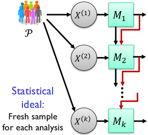
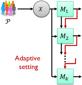
Figure 1: Ideally, we would collecty fresh data from the same population ${\mathcal{P}}$ for each analysis (left). In many real settings, we have only a single data set that must be re-used, leading to adaptively selecected analyses (right). The arrows pointing into the top of the analyses indicate that each analysis is selected based on the results of previous stages.

Our goal is to relate these two settings—to develop techniques that allow us to emulate the ideal world in the real one, and understand how much accuracy is lost due to adaptivity. As mentioned above, merely setting aside a holdout to verify results at each stage is not sufficient, since the holdout ends up being re-used adaptively. If the number $k$ of analyses is known ahead of time, one can split the data into $k$ pieces of $n/k$ points each (assuming i.i.d. data, the pieces are independent). This practice, called data splitting, provides clear validity guarantees, but is inefficient in its use of data: data splitting requires $n$ to be substantially larger than $k$, while we will see techniques that do substantially better. Data splitting also requires an agreed upon partition of the data, which can be problematic with data shared across studies.

A line of work in computer science [21, 28, 20, 19, 40, 41, 6, 39, 46, 23, 24] initiated by Dwork, Feldman, Hardt, Pitassi, Reingold, and Roth [21] and Hardt and Ullman [28] provides a set of tools and specific methodology for this problem. This article briefly surveys the ideas in these works, with emphasis on the role of several information-theoretic concepts. Broadly, there is a strong connection between the extent to which an adaptive sequence of analyses remains faithful to the underlying population ${\mathcal{P}}$, and the amount of information that is leaked to the analyst about ${\mathbf{X}}$. In particular, randomization plays a key role in the state of the art methods, with a notion of algorithmic stability—differential privacy—playing a central role.

Another approach, with roots in the statistics community, seeks to model particular sequences of analyses, designing methodology to adjust for the bias due to conditioning on earlier results (e.g.,  [36, 30, 26, 22, 34, 32]). The specificity of this line of work makes it hard to compare with the more general approaches from computer science. Other work in statistics hews an intermediate path, allowing the analyst freedom within a prespecified class of analyses [7, 10]. There are intriguing similarities between these lines of work and the work surveyed here, such as the use of randomization to break up dependencies (e.g., [42, 43, 29]); understanding these connections more deeply is an important direction for future work.

2 The Lessons of Linear Queries

A simple but important setting for thinking about adaptivity, introduced by Dwork et al. [21] and Hardt and Ullman [28], is that of an analyst posing an adaptively selected sequence of queries, each of which asks for the expectation of a bounded function in the population. Such queries capture a wide range of basic descriptive statistics (the prevalence of a disease in a population, for example, or the average age). Many inference algorithms can also be expressed in terms of a sequence of such queries [31]; for example, optimization algorithms that query the gradient of a Lipschitz, decomposable loss function.

Suppose each data point lies in a universe ${\mathcal{X}}$, so that a data set lies in ${\mathcal{X}}^{n}$ and the underlying population is a distribution on ${\mathcal{X}}$. A bounded linear query is specified by a function $\phi:{\mathcal{X}}\rightarrow[0,1]$. The population value of a linear query is simply the expected value of the function when evaluated on an element of the data universe drawn according to $\mathcal{P}$, denoted $\phi({\mathcal{P}})=\mathbb{E}_{x\sim{\mathcal{P}}}[\phi(x)]$.

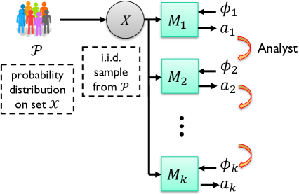
Figure 2: Adaptively selected linear queries

Consider now an interaction between an analyst wishing to pose such queries and an algorithm $M$ (called the mechanism) holding a data set ${\mathbf{X}}$ sample i.i.d from ${\mathcal{P}}$ that attempts to provide approximate answers to the queries $\phi_{1},\phi_{2},...$. This is illustrated in Figure 2, where we use subscripts (as in $M_{1},M_{2},...$) to distinguish $k$ different rounds of $M$. In general, neither the mechanism nor the analyst knows the exact distribution ${\mathcal{P}}$ (otherwise, why collect data?), so the mechanism cannot always answer $\phi({\mathcal{P}})$. A natural approach is to answer with the empirical mean $\phi({\mathbf{X}})=\frac{1}{n}\sum_{x_{i}\in{\mathbf{x}}}\phi(X_{i})$. When queries are selected nonadaptively, this is the best estimator of $\phi({\mathcal{P}})$. We shall see, however, this is not the best mechanism for estimating the expectations of adaptively selected queries!

Given a query answering mechanism $M$, a data analyst $A$, and a distribution ${\mathcal{P}}$ on the data universe ${\mathcal{X}}$, consider a random interaction defined by selecting a sample ${\mathbf{X}}$ of $n$ i.i.d. draws from ${\mathcal{P}}$, and then having $A$ interact with $M({\mathbf{X}})$ for $k$ rounds, where in each round $i$, (i) $A$selects $\phi_{i}$ (based on $a_{1},\ldots,a_{i-1}$), (ii) $M$answers $a_{i}$. The (population) error of $M$ is the random variable

$$\text{\rm err}_{\mathbf{X}}(M,A)=\max_{i}\left|{\phi_{i}({\mathcal{P}})-a_{i}}\right|\,.$$

which depends on ${\mathbf{X}}$ as well as the coins of $M$ and $A$.

Definition 1.

A query answering mechanism $\mathcal{M}$ is $(\alpha,\beta)$-accurate on i.i.d. data for $k$ queries if for every data analyst $A$ and distribution $\mathcal{P}$, we have

$$\Pr{\left({\text{\rm err}_{\mathbf{X}}(M,A)\leq\alpha}\right)}\geq 1-\beta\,.$$

The probability is over the choice of the dataset ${\mathbf{X}}\sim_{\text{i.i.d.}}{\mathcal{P}}$ and the randomness of the mechanism and the analyst. Similarly, the expected error of $M$ is the supremum, over distributions ${\mathcal{P}}$ and data analysts $A$, of $\operatorname*{{\mathbb{E}}}(\text{\rm err}_{\mathbf{X}}(M,A))\,.$ We sometimes fix the distribution ${\mathcal{P}}$ and take the supremum only over analysts $A$.

It is important to note that this definition makes no assumptions on how the analyst selects queries, except that the selection is based on the outputs of $M$ and not directly on the data. The aim of this line of work is to design mechanisms with provable bounds on accuracy. We aim for mechanisms that are universal, in the sense that they can be used in any type of exploratory or adaptive workflow.

2.1 Failures of Straightforward Approaches

As mentioned above, there are a couple of natural approaches to this problem. The first is to answer queries using each query’s empirical mean $\phi({\mathbf{x}})$. When queries are specified nonadaptively, a standard argument shows that the population error of that strategy is $\Theta{\left({\sqrt{(\log k)/n}}\right)}\,.$

In contrast, in the adaptive setting, the empirical mechanism’s error may be unbounded even with just two queries. For example, the query $\phi$ may be selected such that the low-order bits of $\phi_{1}({\mathbf{x}})$ reveal all the entries of the data set ${\mathbf{x}}$. In that case, the analyst may construct a query $\phi_{2}$ which takes the value 1 for values in the data set ${\mathbf{x}}$, and 0 otherwise. The empirical mean $\phi_{2}({\mathbf{x}})$ will be 1, while the population mean $\phi_{2}({\mathcal{P}})$ will be close to 0 for any distribution ${\mathcal{P}}$ with sufficiently high entropy.

This last example seems contrived, since it requires seemingly atypical structure from the initial query $\phi_{1}$. For example, constraining the queries $\phi$ to be predicates taking values in $\{0,1\}$ seems to eliminate the problem. However, the example is instructive for at least two reasons. First, it illustrates the role that information about the data set can play: learning ${\mathbf{x}}$ allows the analyst to pose a query that is highly overfit to the data set, and thus difficult for the mechanism to answer accurately. Conversely, we will see that limiting the information revealed about the data strongly limits overfitting.

Second, when the analyst asks more queries, one can construct much more natural examples of analyses that go awry when using the empirical mean. For instance, consider a data set where each individual data point lies in ${\mathcal{X}}=\{0,1\}^{k-1}\times\{0,1\}$, where we think of the first $k-1$ bits as a vector of binary features, and the last bit as a label. Consider a particular analyst (from [20]) aiming to find a good classification rule for the label. The analyst’s first $k-1$ queries ask for the success rate of each of the $k-1$ features in predicting the label. In the $k$-th query, the analyst constructs a classifier that takes a majority vote among those features that had success rate greater than 50%. On uniformly random data (where the label is independent of the features), the mechanism will report the success rate of this last classifier to be $55\%$ when $k=\frac{n}{10}$, and $67\%$ when $k=n$ (even though its success rate on the population would be $1/2$). Generalizing the example somewhat, one can show that even with very simple data distributions, the error of empirical mechanism scales as $\Theta(\sqrt{k/n})$—exponentially larger than the error one gets with nonadaptively specified queries. Encapsulating this discussion, we have:

Proposition 1.

When answering $k$ nonadaptively specified queries, the empirical mechanism has expected error $\Theta{\left({\sqrt{\log(k)/n}}\right)}$. When answering $k$ adaptively selected queries, the empirical mechanism has expected error $\Omega{\left({\sqrt{k/n}}\right)}$, even for predicate queries on uniformly random data in $\{0,1\}^{k}$.

Data Splitting

Another natural approach for handling adaptively specified queries is data splitting: when $k$ is known in advance, one may divide the data set into $k$ subsamples of $n/k$ points each, and answer the $i$-th query using its empirical mean on the $i$-th data set. This approach means that we can truly ignore adaptivity and use all the tools of classical statistics; the downside is that we are limited to the accuracy one can get with sample size $n/k$. The fact that we want a bound that is uniform over all $k$ queries adds a further logarithmic factor to the final error bound:

Proposition 2.

When answering $k$ adaptively specified queries, the data splitting mechanism has expected error $\Theta(\sqrt{k(\log k)/n})$.

For both of these natural mechanisms, answering queries with error $\alpha$, even with constant probability, requires $n$ to grow at least as fast as $k/\alpha^{2}$. Can we do better? How good a dependency on $\alpha$ and $k$ is possible?

2.2 A Sample of Known Bounds

In fact, there are mechanisms that can answer a sequence of $k$ adaptively selected linear queries with much higher accuracy than that provided by the straightforward approaches. Namely, for a given accuracy $\alpha$, we can get mechanisms that work for $n$ that scales only as $\sqrt{k}/\alpha^{2}$—a quadratic improvement in $k$. The bounds below are stated in terms of expected error for simplicity; the underlying arguments also provide high-probability bounds on the tail of this error.

Theorem 3 ([21, 6]).

There is a computationally efficient mechanism for $k$ statistical queries with expected error $O{\left({\sqrt[4]{k}/\sqrt{n}}\right)}$.

A simple mechanism that achieves this bound is one that adds Gaussian noise with standard deviation about $\sqrt[4]{k}/\sqrt{n}$ to each query.

One can give a different-looking mechanism—which we do not describe in this survey—to automatically adjust to the actual “amount” of adaptivity in a given sequence of queries. Specifically, imagine that the $k$ queries are grouped into $r$ batches, where the queries in a given batch depend on answers to queries in previous batches but not on the answers to queries in the same batch. For example, in the classification example of the previous section, the number of rounds $r$ is only $2$.

Theorem 4 ([21]).

If there are at most $r$ rounds of adaptivity, then there is a computationally efficient mechanism with expected error $O{\left({\sqrt{r(\log k)/n}}\right)}$. The algorithm is not given the partition of the queries into batches.

The ideas underlying the two previous algorithms can also be adapted to give better results when we make further assumptions about the class of allowed queries, or the universe from which the data are drawn. One such result, due to Dwork et al. [21] (and tightened in [6]), recovers a logarithmic dependence on $k$ in exchange for a dependence on the size of the universe ${\mathcal{X}}$ in which the data lie.

Theorem 5 ([21, 6]).

There is a computationally inefficient mechanism with expected error
$O{\left({\sqrt[6]{\log|{\mathcal{X}}|}\sqrt[3]{(\log k)/n}}\right)}$. The mechanism runs in time linear in $|{\mathcal{X}}|$ (and not $\log|{\mathcal{X}}|$ as one would naturally want).

None of these upper bounds is known to be tight in all parameter regimes, but some lower bounds are known, in particular showing that the scaling $n=\Omega(\sqrt{k})$ cannot be improved, and that inefficiency of the mechanism in Theorem 5 is necessary.

Theorem 6 (Hardt and Ullman [28], Steinke and Ullman [41]).

For every mechanism $M$ that answers $k$ adaptively selected linear queries, for a sufficiently large universe ${\mathcal{X}}$ (with $\log|{\mathcal{X}}|$ exponential in $n$), there exist a distribution ${\mathcal{P}}$ and an analyst ${\mathcal{A}}$ for which the mechanism’s error $\text{\rm err}_{{\mathbf{X}}}(M,A)$ is $\Omega{\left({\sqrt{k}/n}\right)}$ with constant probability. Furthermore, for mechanisms that answer faithfully with respect to both the distribution and the data set (that is, they provide answers close to both $\phi_{i}({\mathbf{X}})$ and $\phi_{i}({\mathcal{P}})$), the bound can be strengthened to $\Omega{\left({\sqrt[4]{k}/\sqrt{n}}\right)}$

Finally, if we assume that one-way functions exist, then the bounds continue to hold when $\log|{\mathcal{X}}|$ has polynomial size, for polynomial-time mechanisms (but not for those that can take exponential time).

We won’t discuss the proof of these lower bounds here, but we note that closing the gap between the upper and lower bounds remains an intriguing open problem.

2.3 Privacy and Distributional Stability

The upper bounds above are obtained via a connection between adaptive analysis and certain notions of algorithmic stability. Broadly, algorithmic stability properties limit how much the output of an algorithm can change when one of its inputs is changed. Different notions of stability correspond, roughly, to different measures of distance between outputs. There is a long-standing connection between algorithmic stability and expected generalization error (e.g., Devroye and Wagner [14], Bousquet and Elisseeff [9]). Essentially, stable algorithms cannot overfit. It seems that if we could design adaptive query-answering mechanisms that are stable in an appropriate sense, we could get validity guarantees for adaptive data analysis.

Alas, there is a hitch. Recall that our goal is to design mechanisms that provide statistically valid answers no matter how the analyst selects queries. Even if each stage of the mechanism is stable, the overall process might not be—in an adaptive setting, the analyst ends up being part of the mechanism.

The resolution is to consider a distributional notion of stability. We will require that changing any single data point in ${\mathbf{x}}$ have a small effect on the distribution of the mechanism’s outputs. If we choose a distance measure on distributions that is nonincreasing under postprocessing, then we can limit the effect of the analyst’s choices.

Specifically, we work with “differential privacy”, a notion of stability introduced in the context of privacy of statistical data. Differential privacy seeks to limit the information revealed about any single individual in the data set.

Definition 2 ([17, 16]).

An algorithm $M:{\mathcal{X}}^{n}\rightarrow\mathcal{O}$ is $(\epsilon,\delta)$-differentially private if for all pairs of neighboring data sets ${\mathbf{x}},{\mathbf{x}}^{\prime}\in{\mathcal{X}}^{n}$, and for all events $S\subseteq\mathcal{O}$:

$$\Pr[M({\mathbf{x}})\in S]\leq\exp(\epsilon)\Pr[M({\mathbf{x}}^{\prime})\in S]+\delta\,.$$

Differential privacy makes sense even for interactive mechanisms that involve communication with an outside party: we simply think of the outside party as part of the mechanism, and define the final output of the mechanism to be the complete transcript of the communication between the mechanism and the other party.

Differential privacy is a useful design tool in the context of adaptive data analysis because it is possible to design interactive differentially private algorithms modularly, due to two related properties: closure under postprocessing, and composition:

Proposition 7.

If $M:{\mathcal{X}}^{n}\rightarrow\mathcal{O}$ is $(\epsilon,\delta)$-differentially private, and $f:\mathcal{O}\rightarrow\mathcal{O}^{\prime}$ is an arbitrary (possibly randomized) mapping, then $f\circ M:{\mathcal{X}}^{n}\rightarrow\mathcal{O}^{\prime}$ is $(\epsilon,\delta)$-differentially private.

Proposition 8 (Adaptive Composition [18, 35]—informal).

Let $M_{1},M_{2},...,M_{k}$ be a sequence of $(\epsilon,\delta)$-differentially private algorithms that are all run on the same data set, and selected adaptively (with the choice of $M_{i}$ depending on the outputs of $M_{1},...,M_{i-1}$, but not directly on ${\mathbf{x}}$). Then no matter how the adaptive selection is done, the resulting composed process is $(\epsilon^{\prime},\delta^{\prime})$-differentially private, for $\epsilon^{\prime}\approx\epsilon\sqrt{k}$ and $\delta^{\prime}\approx k\delta$.

Taken together, these two properties mean that in order to design differentially private algorithms for answering linear queries, it is sufficient to make sure the mechanism run at each stage is differentially private.

Perhaps even more importantly, in order to ensure statistical validity—that is, accuracy with respect to the underlying population—it suffices to design differentially private algorithms that are accurate with respect to the sample ${\mathbf{x}}$:

Theorem 9 (Main Transfer Theorem [21, 6]).

Suppose a statistical estimator $M$ is $(\epsilon,\epsilon\cdot\delta)$-accurate with respect to its sample, that is, for all data sets ${\mathbf{x}}$,

$$\Pr(\max_{i}\left|a_{i}-\phi_{i}({\mathbf{x}})\right|\leq\epsilon)\geq 1-\epsilon\cdot\delta\,.$$

If $M$ is also $(\epsilon,\epsilon\cdot\delta)$-differentially private, then it is $(O(\epsilon),O(\delta))$-accurate with respect to the population (Definition 1).

This theorem underlies all two of the three upper bounds of the previous section (Theorems 3 and 5). Each is derived by using existing differentially private algorithms together with Theorem 9. For Theorem 4, Dwork et al. [21] used a different argument, based on compressing the output of the algorithm to a small set of possibilities; see Section 3.

2.4 A Two-stage Game, Stability and “Lifting”

We conclude this section with an outline of the proof of the main transfer theorem (Theorem 9). That theorem talks about analyses with many stages of interaction, but it turns out that the core of the argument lies in understanding a seemingly much simpler, two-stage process.

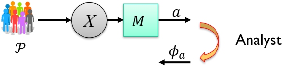
Figure 3: A two-stage overfitting game

Consider a two-stage setting in which an analysis $M$ is run on data set ${\mathbf{x}}$, and the analyst selects a linear query $\phi:{\mathcal{X}}\to[0,1]$ based on $M({\mathbf{x}})$ (Figure 3). We say $M$ robustly $(\alpha,\beta)$-generalizes if for all distributions ${\mathcal{P}}$ over the domain ${\mathcal{X}}$, for all strategies (functions) $A$ employed by the analyst, with probability at least $1-\beta$ over the choice of ${\mathbf{X}}\sim{\mathcal{P}}^{n}$ and the coins of $M$, we have that $|\phi({\mathbf{X}})-\phi({\mathcal{P}})|\leq\alpha$ where $\phi=A(M({\mathbf{X}}))$. (Similarly, we may talk about the expected generalization error, that is, the maximum over $A$ and ${\mathcal{P}}$ of $\operatorname*{{\mathbb{E}}}(|\phi({\mathbf{X}})-\phi({\mathcal{P}})|)$.)

The quantification over all selection functions $A$ here is critical—when the first phase of analysis satisfies the definition, then a query asked in the following round cannot overfit to the data (except with low probability), no matter how it is selected.

Differential privacy (and a few other distributional notions of stability, such as KL-stability [6, 47]) limits the adversary’s score in this game. This connection had been understood for some time—for example, McSherry observed that it could be used to break up dependencies in a clustering algorithm, and Bassily et al. [5] used a weak version of the connection to bound the population risk of differentially private empirical risk minimization.

However, the application to adaptive data analysis–and especially the understanding of the importance of post-processing to the design of universal mechanisms—came recently, in [21]. Their initial result was subsequently sharpened, to obtain the following tight connection:

Theorem 10 (Differentially Private Algorithms Cannot Overfit [6]).

If $M$ is $(\epsilon,\epsilon\delta)$-differentially private, then it is $(O(\epsilon),O(\delta))$-robustly generalizing.

Lifting to Many Stages

Bounds on the two-stage game can be “lifted” to provide bounds on the $k$-phase game either through a sequential application of the bound to each round [21] or through a more holistic argument, called the monitor technique [6], that yields Theorem 9 (and Theorems 3 and 5).

The monitor argument is a thought experiment—we argue that for any multi-stage process, there is a two-stage process in which the error on the population equals the maximum population error over all $k$ stages of the original process. The argument applies quite generally, but it is a bit simpler to explain under the assumption that the mechanism answers queries accurately with respect to the data set ${\mathbf{X}}$. The idea, given an interaction between an analyst and adaptively selected mechanisms $M_{1},M_{2},...,M_{k}$, is to encapsulate the analyst and mechanisms into a single fictional entity $M$ which gets, as additional input, the underlying distribution ${\mathcal{P}}$. The fictional $M$ executes an interaction and then outputs a single query $\phi^{*}$—the one which maximizes the population error over all stages $i$.

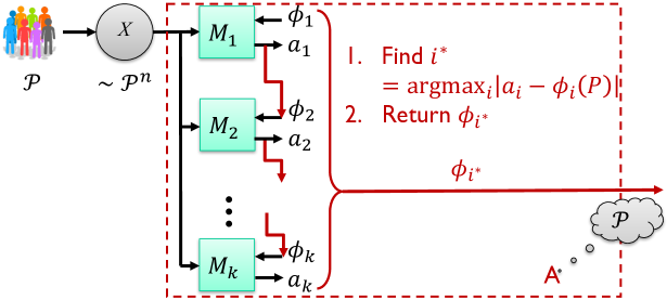
Figure 4: The “monitor” argument for lifting results about a two-stage game to many stages

Beyond linear queries

The techniques described in this section extend to problems that are not described by estimating the mean of a bounded linear functional. One important class is minimizing a decomposable loss function where each individual contributes a bounded term to the loss function [6].

A re-usable holdout

The techniques described in this section can appear somewhat onerous for the analyst, since they require accessing data via differentially private algorithms. As pointed out by Dwork et al. [20], however, one need not limit access to the entire data set in this way. In fact, a more pragmatic approach is to give most of the data “in the clear” to the analyst, and protect only a small holdout set via the techniques discussed here. This still allows one to verify conclusions soundly, but additionally allows full exploratory analysis, as well as repeated verification (“holdout re-use”).

3 The Intrigue of Information Measures

Despite the generality of the approach of the previous section, many important classes of analyses are not obviously amenable to those techniques; in particular, problems that are not easily stated in terms of a numerical estimation task.

Consider the problem of hypothesis testing. Crudely, given a set of distributions ${\mathcal{H}}$ (called the null hypothesis), we ask if the data set is “unlikely to have been generated” by a distribution $P\in{\mathcal{H}}$. More precisely, we select an event $T$ (the acceptance region) such that $\Pr_{{\mathbf{X}}\sim{\mathcal{P}}^{n}}({\mathbf{X}}\in T)$ is at most a threshold $\gamma$ (often 0.05) for all distributions in ${\mathcal{H}}$. If it happens that the observed data ${\mathbf{X}}$ lie outside of $T$, the null hypothesis is said to be rejected. If this happens when the true distribution ${\mathcal{P}}$ is actually in ${\mathcal{H}}$, then we say a false discovery occurs. Hypothesis tests play a central role in modern empirical science (for better or for worse), and techniques to control false discovery in the classic, nonadaptive setting are the focus of intense study. Despite this, very little is known about hypothesis tests in adaptive settings.

Adaptivity arises when the event $T$ is selected based on earlier analysis of the same data – conditioned on those earlier results $Y=M({\mathbf{X}})$, the probability that the test rejects the null hpyothesis given ${\mathbf{X}}$ might be much higher than $\gamma$ even if ${\mathcal{P}}$ lies in ${\mathcal{H}}$.

How much higher it can be depends on $M$ and—as we will see—on several measures of the information leaked by $M$. To formalize this, consider a game similar to the overfitting game, in which the analyst $A$, given $Y=M({\mathbf{X}})$, selects an arbitrary event $T_{Y}=A(Y)$ (which depends on $Y$). For a particular output $y$ of $M$, the analyst’s “score” is

$$\text{score}_{{\mathcal{P}},M,A,\gamma}(y)=\begin{cases}\Pr_{{\mathbf{X}}\sim{\mathcal{P}}^{n}}({\mathbf{X}}\in T_{y}|Y=y)&\text{if }\Pr_{{\mathbf{X}}\sim{\mathcal{P}}^{n}}({\mathbf{X}}\in T_{y})\leq\gamma\,,\\ 0&\text{if }\Pr_{{\mathbf{X}}\sim{\mathcal{P}}^{n}}({\mathbf{X}}\in T_{y})>\gamma\,.\end{cases}$$

Now consider the analyst’s expected score in this game: $\displaystyle\eta_{{\mathcal{P}},M,A}(\gamma)=\operatorname*{{\mathbb{E}}}_{Y}\big{(}\text{score}_{{\mathcal{P}},M,A}(y)\big{)}$. As we will see below, the analyst’s score in this game can be bounded using various definitions of the information leaked about ${\mathbf{X}}$ by $Y$. This score also plays a key role in controlling false discovery:

Proposition 11.

Bounding the score $\eta$ has several important implications:

1. (False discovery [39]) If $Y=M({\mathbf{X}})$ is used by $A$ to select a hypothesis test with significance $\gamma$, then the probability of false discovery is at most $\eta_{{\mathcal{P}},M,A}(\gamma)$.

2. (Robust generalization [19]) If $Y=M({\mathbf{X}})$ is used by $A$ to select a bounded linear query $\phi_{Y}$, then $\Pr{\big{(}{\left|\phi_{Y}({\mathbf{X}})-\phi_{Y}({\mathcal{P}})\right|\geq t/\sqrt{n}}\big{)}}\leq\eta_{{\mathcal{P}},M,A}\left(e^{-t^{2}/3}\right)$.

We are interested in universal bounds that hold no matter how the analyst uses the output $Y$, and no matter the original input distribution. To this end, we define

$$\eta_{M}(\gamma)=\sup_{{\mathcal{P}},A}\left(\eta_{{\mathcal{P}},M,A}(\gamma)\right)\,.$$

3.1 Information and Conditioning

The function $\eta_{M}$ measures how much probabilities less than $\gamma$ can be amplified by conditioning on $Y$, on average over values of $Y$.

For several one-shot notions of mutual information, we have that if a procedure leaks $k$ “bits” of information we have $\eta_{{\mathcal{P}},M,A}(\gamma)\approx\gamma\cdot 2^{k}$. Unfortunately, such a clean relationship is not known for the standard notion of Shannon mutual information. Instead, we consider two other notions here.

Fix two random variables $X,Y$ with joint distribution given by $p_{XY}(x,y)=\Pr(X=x,Y=y)$ and marginals $p_{X}(\cdot)$ and $p_{Y}(\cdot)$. Consider the information loss

$$I_{x,y}=\log\left(\frac{p_{XY}(x,y)}{p_{X}(x)p_{Y}(y)}\right)\,.$$

The standard notion of mutual information is the expectation of this variable: $I(X;Y)=\operatorname*{{\mathbb{E}}}\left(I_{X,Y}\right)$. The max-information [12, 19] between $X$ and $Y$ is the supremum of this variable. Unfortunately, for many interesting procedures, the max-information is either unbounded or much larger than the mutual information.

One can get a more flexible notion by instead considering a high-probability bound on the information loss: we say the $\beta$-approximate max information between $X$ and $Y$ is at most $k$ (written $I_{\infty}^{\beta}(X;Y)\leq k$) if $\Pr_{(x,y)\sim(X,Y)}(I_{x,y}\leq k)\geq 1-\beta$.  

For many algorithms of interest, the approximate max-information turns out to be very close to the mutual information but, by providing a bound on the upper tail of $I_{X,Y}$, allows for more precise control of small-probability events.

We can also define a related quantity, which we call the expected log-distortion:

$$L_{\infty}(X;Y)=\log\operatorname*{{\mathbb{E}}}_{y\sim Y}\left(\sup_{x}\left(2^{I_{x,y}}\right)\right)=\log\operatorname*{{\mathbb{E}}}_{y\sim Y}\left(\sup_{x}\frac{p_{XY}(x,y)}{p_{X}(x)p_{Y}(y)}\right)\,.$$

This notion of information leakage is not symmetric in $X,Y$. It is closely related to, but in general different from, the min-entropy leakage $H_{\infty}(Y|X)-H_{\infty}(X)$  [15, 1, 25, 2, 3].

Of these notions, expected log distortion is the strongest since it upper bounds the other two: $I(X;Y)\leq L_{\infty}(X;Y)$ and $I_{\infty}^{\beta}(X;Y)\leq L_{\infty}(X;Y)+\log(1/\beta)$.

Theorem 12.

For every mechanism $M$ and dsitribution ${\mathcal{P}}$ s.t. ${\mathbf{X}}\sim{\mathcal{P}}$:

1. If $I_{\infty}^{\beta}({\mathbf{X}};Y)\leq k$, then for every analyst $A$, $\eta_{{\mathcal{P}},M,A}(\gamma)\leq\gamma\cdot 2^{k}+\beta$, and
   $M$ robustly $(\alpha,2\beta)$-generalizes for $\alpha=\sqrt{(k+2\ln(1/\beta))/n}$ on ${\mathcal{P}}$.

2. If $L_{\infty}({\mathbf{X}};M({\mathbf{X}}))\leq k$, then for every analyst $A$, $\eta_{{\mathcal{P}},M,A}(\gamma)\leq\gamma\cdot 2^{k}$, and
   for every $\beta>0$, $M$ robustly $(\alpha,\beta)$-generalizes for $\alpha=\sqrt{(k+2\ln(1/\beta))/n}$ on ${\mathcal{P}}$.

We know much weaker implications based only on bounding the mutual information. Most significantly, the bounds for general hypothesis testing are exponentially weaker than those one gets from the one-shot measures above.

Proposition 13 ([40, 39]).

If $I({\mathbf{X}};M({\mathbf{X}}))\leq k$, then (i) for every analyst $A$, $\eta_{{\mathcal{P}},M,A}(\gamma)\leq\frac{k+1}{\log_{2}(1/\gamma)}$, and (ii) for every $\beta>0$, $M$ robustly $(\alpha,\beta)$-generalizes for $\alpha=O(\sqrt{k/n\beta})$ on ${\mathcal{P}}$.

3.2 What procedures have bounded one-shot information measures?

The information-theoretic framework of the previous subsection captures several other classes of algorithms that satisfy robust generalization guarantees. In addition to unifying the previous work, this approach shows that these classes of algorithms allow for principled post-selection hypothesis testing.

The most important of these, currently, is for the class of differentially private algorithms:

Theorem 14 (Informal, see [39]).

If $M$ is $(\epsilon,\delta)$-differentially private, and the entries of ${\mathbf{X}}$ are independent, then $I_{\infty}^{\beta}({\mathbf{X}};M({\mathbf{X}}))=O(\epsilon^{2}n)$ for $\beta=O(n\sqrt{\delta/\epsilon})$.

This result, together with Theorem 12, implies that differentially-private algorithms are $(O(\epsilon),O(n\sqrt{\delta/\epsilon})$-robustly generalizing for data drawn i.i.d from any distribution ${\mathcal{P}}$. It essentially recovers the results of the previous section on linear queries (with a worse value of $\beta$), but additionally applies to more general problems such as hypothesis testing.

Description length [19]

In many cases, the outcome of a statistical analysis can be compressed to relatively few bits—for example, when the outcome is a small set of selected features. If the output of $M$ can be compressed to $k$ bits, then the expected log-distortion $L_{\infty}({\mathbf{X}};M({\mathbf{X}}))$ is at most $k$ bits. An argument along these lines was used implicitly in [21] to prove Theorem 4.

Compression Schemes

Another important class of statistical analyses that have good (and robust) generalization properties are compression learners [33]. These process a data set of $n$ points to obtain a carefully selected subset of only $k<<n$ points, and finally produce an output fit to those points. A classic example is support vector machines: in $d$ dimensions, the final classifier is determined by just $d+1$ points in the data set.

Cummings et al. [13] used classic generalization results for such learners to show that they satisfy robust generalization guarantees. The classic results as well as those of Cummings et al. [13] can be rederived from the following lemma (new, as far as we know) bounding the information leaked by a compression scheme about those points that are not output by the scheme.

Lemma 15 (Compression schemes).

Let $M:{\mathcal{X}}^{n}\to{\mathcal{X}}^{k}$ be any algorithm that takes a data set ${\mathbf{x}}$ of $n$ points and outputs a subset ${\mathbf{x}}_{out}=M({\mathbf{x}})$ of $k$ points from ${\mathbf{x}}$. Let ${\mathbf{x}}_{in}\in{\mathcal{X}}^{n-k}$ denote the remaining data points, so that ${\mathbf{x}}_{in}\cup{\mathbf{x}}_{out}={\mathbf{x}}$ (as multisets). For any distribution ${\mathcal{P}}$ on ${\mathcal{X}}$, if ${\mathbf{X}}\sim{\mathcal{P}}^{n}$, then

$$L_{\infty}({\mathbf{X}}_{in};{\mathbf{X}}_{out})\leq\log_{2}\binom{n}{k}\,.$$

Cummings et al. [13] used the robust generalization properties of compression learners to give robustly generalizing algorithms for learning any PAC-learnable concept class. In particular, this implies robustly generalizing algorithms for tasks that do not have differentially private algorithms, such as learning a threshold classifier with data from the real line.

Notes and Acknowledgments

I am grateful to many colleagues for introducing me to this topic and insightful discussions. Among others, my thanks go to Raef Bassily, Cynthia Dwork, Moritz Hardt, Kobbi Nissim, Ryan Rogers, Aaron Roth, Thomas Steinke, Uri Stemmer, Om Thakkar, Jon Ullman, Yu-Xiang Wang. Paul Medvedev provided helpful comments on the writing, making the survey a tiny bit more accessible to nonexperts. Finally, I thank Michael Langberg, this newsletter’s editor, for soliciting this article and graciously tolerating delays in its preparation.

Although I tried to cover the main ideas in a recent line of work, that line is now diverse enough that I could not encapsulate everything here. Notable omissions include the “jointly Gaussian” models of Russo and Zou [40] and Wang et al. [46], which assume that the analyst is selecting among a family of statistics that are jointly normally distributed under ${\mathcal{P}}$ , work of Elder [23, 24] on a Bayesian framework that encodes a further restriction that the mechanism “know as much” as the analyst about the underlying distribution ${\mathcal{P}}$, and the “typcial stability” framework [4, 13]. There are no doubt other contributions that I lost in my effort to consolidate. Some ideas in this survey, notably the information-theoretic viewpoint on compression-based learning, have not appeared elsewhere; they have not been peer-reviewed.

References

- Alvim et al. [2012] M. S. Alvim, K. Chatzikokolakis, C. Palamidessi, and G. Smith. Measuring information leakage using generalized gain functions. In 25th IEEE Computer Security Foundations Symposium (CSF), pages 265–279, 2012.
- Alvim et al. [2014] M. S. Alvim, K. Chatzikokolakis, A. McIver, C. Morgan, C. Palamidessi, and G. Smith. Additive and multiplicative notions of leakage, and their capacities. In 27th IEEE Computer Security Foundations Symposium (CSF), pages 308–322, 2014.
- Alvim et al. [2016] M. S. Alvim, K. Chatzikokolakis, A. McIver, C. Morgan, C. Palamidessi, and G. Smith. Axioms for information leakage. In 29th IEEE Computer Security Foundations Symposium (CSF), pages 77–92, 2016.
- Bassily and Freund [2016] R. Bassily and Y. Freund. Typical stability. arXiv:1604.03336 [cs.LG], April 2016.
- Bassily et al. [2014] R. Bassily, A. Smith, and A. Thakurta. Private empirical risk minimization: Efficient algorithms and tight error bounds. In IEEE Symposium on the Foundations of Computer Science (FOCS), pages 464–473, 2014.
- Bassily et al. [2016] R. Bassily, K. Nissim, A. Smith, T. Steinke, U. Stemmer, and J. Ullman. Algorithmic stability for adaptive data analysis. In 48th Annual ACM SIGACT Symposium on Theory of Computing, pages 1046–1059, 2016.
- Berk et al. [2013] R. Berk, L. Brown, A. Buja, K. Zhang, and L. Zhao. Valid post-selection inference. The Annals of Statistics, 41(2):802–837, 2013.
- Blum and Hardt [2015] A. Blum and M. Hardt. The ladder: A reliable leaderboard for machine learning competitions. In Proc. 32 nd International Conference on Machine Learning, 2015. arXiv:1502.04585.
- Bousquet and Elisseeff [2002] O. Bousquet and A. Elisseeff. Stability and generalization. Journal of Machine Learning Research, 2:499–526, 2002.
- Buja et al. [2015] A. Buja, R. Berk, L. Brown, E. George, E. Pitkin, M. Traskin, L. Zhao, and K. Zhang. Models as approximations—a conspiracy of random regressors and model deviations against classical inference in regression. Statistical Science, 1460, 2015.
- Bun and Steinke [2016] M. Bun and T. Steinke. Concentrated differential privacy: Simplifications, extensions, and lower bounds. In Theory of Cryptography Conference (TCC) 2016-B, 2016. arxiv:1605.02065.
- Ciganovic et al. [2014] N. Ciganovic, N. J. Beaudry, and R. Renner. Smooth max-information as one-shot generalization for mutual information. IEEE Trans. Information Theory, 60(3):1573–1581, 2014.
- Cummings et al. [2016] R. Cummings, K. Ligett, K. Nissim, A. Roth, and Z. S. Wu. Adaptive learning with robust generalization guarantees. In 29th Annual Conference on Learning Theory, pages 772–814, 2016.
- Devroye and Wagner [1979] L. Devroye and T. Wagner. Distribution-free performance bounds for potential function rules. IEEE Transactions on Information Theory, 25(5):601–604, 1979.
- Dodis et al. [2008] Y. Dodis, R. Ostrovsky, L. Reyzin, and A. Smith. Fuzzy extractors: How to generate strong keys from biometrics and other noisy data. SIAM J. Comput., 38(1):97–139, 2008.
- Dwork et al. [2006a] C. Dwork, K. Kenthapadi, F. McSherry, I. Mironov, and M. Naor. Our data, ourselves: Privacy via distributed noise generation. In Advances in Cryptology - EUROCRYPT, pages 486–503, St. Petersburg, Russia, 2006a.
- Dwork et al. [2006b] C. Dwork, F. McSherry, K. Nissim, and A. Smith. Calibrating noise to sensitivity in private data analysis. In Theory of Cryptography Conference, pages 265–284. Springer, 2006b.
- Dwork et al. [2010] C. Dwork, G. N. Rothblum, and S. Vadhan. Boosting and differential privacy. In Proceedings of the 2010 IEEE 51st Annual Symposium on Foundations of Computer Science, FOCS ’10, pages 51–60, Washington, DC, USA, 2010. IEEE Computer Society.
- Dwork et al. [2015a] C. Dwork, V. Feldman, M. Hardt, T. Pitassi, O. Reingold, and A. Roth. Generalization in adaptive data analysis and holdout reuse. In Advances in Neural Information Processing Systems, pages 2350–2358, 2015a.
- Dwork et al. [2015b] C. Dwork, V. Feldman, M. Hardt, T. Pitassi, O. Reingold, and A. Roth. The reusable holdout: Preserving validity in adaptive data analysis. Science, 349(6248):636–638, 2015b.
- Dwork et al. [2015c] C. Dwork, V. Feldman, M. Hardt, T. Pitassi, O. Reingold, and A. L. Roth. Preserving statistical validity in adaptive data analysis. In Proceedings of the Forty-Seventh Annual ACM on Symposium on Theory of Computing, pages 117–126. ACM, 2015c.
- Efron [2014] B. Efron. Estimation and accuracy after model selection. Journal of the American Statistical Association, 109(507):991–1007, 2014.
- Elder [2016a] S. Elder. Challenges in bayesian adaptive data analysis. arXiv:1604.02492, 2016a.
- Elder [2016b] S. Elder. Bayesian adaptive data analysis guarantees from subgaussianity. arXiv:1611.00065 [cs.LG], 2016b.
- Espinoza and Smith [2013] B. Espinoza and G. Smith. Min-entropy as a resource. Inf. Comput., 226:57–75, 2013.
- Fithian et al. [2014] W. Fithian, D. Sun, and J. Taylor. Optimal inference after model selection. arXiv preprint arXiv:1410.2597, 2014.
- Gelman and Loken [2014] A. Gelman and E. Loken. The statistical crisis in science. American Scientist, 102(6):460, 2014.
- Hardt and Ullman [2014] M. Hardt and J. Ullman. Preventing false discovery in interactive data analysis is hard. In Foundations of Computer Science (FOCS), 2014 IEEE 55th Annual Symposium on, pages 454–463. IEEE, 2014.
- Harris et al. [2016] X. T. Harris, S. Panigrahi, J. Markovic, N. Bi, and J. Taylor. Selective sampling after solving a convex problem. arXiv: 1609.05609, 2016.
- Hurvich and Tsai [1990] C. M. Hurvich and C.-L. Tsai. The impact of model selection on inference in linear regression. The American Statistician, 44(3):214–217, 1990.
- Kearns [1998] M. Kearns. Efficient noise-tolerant learning from statistical queries. Journal of the ACM (JACM), 45(6):983–1006, 1998.
- Lee et al. [2016] J. D. Lee, D. L. Sun, Y. Sun, and J. E. Taylor. Exact post-selection inference, with application to the lasso. The Annals of Statistics, 44(3):907–927, 2016.
- Littlestone and Warmuth [1986] N. Littlestone and M. Warmuth. Relating data compression and learnability. Technical report, 1986.
- Lockhart et al. [2014] R. Lockhart, J. Taylor, R. J. Tibshirani, and R. Tibshirani. A significance test for the lasso. The Annals of Statistics, 42(2):413, 2014.
- Oh and Viswanath [2013] S. Oh and P. Viswanath. The composition theorem for differential privacy. CoRR, abs/1311.0776, 2013. URL http://arxiv.org/abs/1311.0776.
- Pötscher [1991] B. M. Pötscher. Effects of model selection on inference. Econometric Theory, 7(2):163–185, 1991.
- Renner and Wolf [2004] R. Renner and S. Wolf. Smooth Rényi entropy and applications. In IEEE International Symposium on Information Theory — ISIT, page 233, 2004.
- Renner and Wolf [2005] R. Renner and S. Wolf. Simple and tight bounds for information reconciliation and privacy amplification. In Advances in Cryptology - ASIACRYPT, pages 199–216, 2005.
- Rogers et al. [2016] R. Rogers, A. Roth, A. Smith, and O. Thakkar. Max-information, differential privacy, and post-selection hypothesis testing. In Foundations of Computer Science (FOCS), 2016 IEEE 57th Annual Symposium on, 2016.
- Russo and Zou [2016] D. Russo and J. Zou. Controlling bias in adaptive data analysis using information theory. In 19th International Conference on Artificial Intelligence and Statistics, pages 1232–1240, 2016. arXiv:1511.05219.
- Steinke and Ullman [2015] T. Steinke and J. Ullman. Interactive fingerprinting codes and the hardness of preventing false discovery. In Proceedings of The 28th Conference on Learning Theory, pages 1588–1628, 2015.
- Tian and Taylor [2015] X. Tian and J. E. Taylor. Selective inference with a randomized response. arXiv:1507.06739, 2015.
- Tian et al. [2016] X. Tian, N. Bi, and J. Taylor. Magic: a general, powerful and tractable method for selective inference. arXiv: 1607.02630, 2016.
- Tomamichel et al. [2010] M. Tomamichel, R. Colbeck, and R. Renner. Duality between smooth min- and max-entropies. IEEE Trans. Information Theory, 56(9):4674–4681, 2010.
- Vitanov et al. [2013] A. Vitanov, F. Dupuis, M. Tomamichel, and R. Renner. Chain rules for smooth min- and max-entropies. IEEE Trans. Information Theory, 59(5):2603–2612, 2013.
- Wang et al. [2016a] Y.-X. Wang, J. Lei, and S. E. Fienberg. A minimax theory for adaptive data analysis. arXiv:1602.04287 [stat.ML], 2016a.
- Wang et al. [2016b] Y.-X. Wang, J. Lei, and S. E. Fienberg. On-average KL-privacy and its equivalence to generalization for max-entropy mechanisms. arXiv:1605.02277 [stat.ML], 2016b.