Streaming Bayesian inference: theoretical limits and
mini-batch approximate message-passing

Abstract

In statistical learning for real-world large-scale data problems, one must often resort to “streaming” algorithms which operate sequentially on small batches of data. In this work, we present an analysis of the information-theoretic limits of mini-batch inference in the context of generalized linear models and low-rank matrix factorization. In a controlled Bayes-optimal setting, we characterize the optimal performance and phase transitions as a function of mini-batch size. We base part of our results on a detailed analysis of a mini-batch version of the approximate message-passing algorithm (Mini-AMP), which we introduce. Additionally, we show that this theoretical optimality carries over into real-data problems by illustrating that Mini-AMP is competitive with standard streaming algorithms for clustering.

1 Introduction

In current machine learning applications, one often faces the challenge of scale: massive data causes algorithms to explode in time and memory requirements. In such cases, when it is infeasible to process the full dataset simultaneously, one must resort to "online" or "streaming" methods which process only a small fraction of data points at a time — producing a step-by-step learning process. Such procedures are becoming more and more necessary to cope with massive datasets. For example, one can see the effectiveness of such approaches in deep learning via the stochastic gradient descent algorithm [1] or in statistical inference via the stochastic variational inference framework [2].

In this work, we treat streaming inference within a Bayesian framework where, as new data arrives, posterior beliefs are updated according to Bayes’ rule. One well known approach in this direction is assumed density filtering (ADF) [3, 4], which processes a single data point at a time, a procedure to which we refer to as fully online. A number of other works analyzed various related fully online algorithms [5, 6], especially in the statistical physics literature [7, 8, 9, 10, 11]. We are instead interested in the case where multiple samples – a mini-batch – arrive at once. Tuning the size of these mini-batches allows us to to explore the trade-off between the precision and efficiency.

Our motivation and setting are very much along the lines of streaming variational Bayes (VB) inference [12]. With respect to existing works, we bring three main contributions. (i) We introduce a streaming algorithm based on approximate message passing (AMP) [13, 14, 15] that we call Mini-AMP. As AMP treats some of the correlations which VB neglects, it is expected that AMP either outperforms or matches VB. (ii) Unlike other general-purpose algorithms for Bayesian inference, such as Gibbs sampling or VB, AMP possesses the state evolution method which asymptotically describes the performance of the algorithm for a class of generative models. We extend this state evolution analysis to Mini-AMP. (iii) For these generative models, we also analyze the optimal streaming procedure, within a class of procedures that retains only point-wise marginals from one step to another, and characterize regions of parameters where Mini-AMP reaches optimality.

2 Problem setting

Denoting the vector of $N$ values to be estimated by $\bm{x}$, the data presented at step $k$ by $\bm{y}^{(k)}$, and the collection of all previously presented data by $\mathcal{D}^{(k-1)}=\{\bm{y}^{(1)},\dots,\bm{y}^{(k-1)}\}$, the posterior distribution at step $k$ is given by

$$P(\bm{x}|\bm{y}^{(k)},\mathcal{D}^{(k-1)})=\frac{P(\bm{y}^{(k)}|\bm{x})\,P(\bm{x}|\mathcal{D}^{(k-1)})}{\int d\bm{x}\,P(\bm{y}^{(k)}|\bm{x})\,P(\bm{x}|\mathcal{D}^{(k-1)})}.$$ (1)

In other words, with each presentation of new data, the prior distribution is updated with the posterior distribution derived from the previously presented data. Directly implementing this strategy is seldom feasible as the normalizing integral in (1) is intractable in general. Additionally, to keep the memory requirements small, we would like consider only the case where $O(N)$ parameters are passed from one step to the next. With this restriction, one cannot carry over high-order correlations from previous steps. Instead, following the strategy of [12], we resort to a factorized approximation of the "prior" term of (1),

$$P(\bm{x}|\mathcal{D}^{(k-1)})\approx Q^{(k-1)}(\bm{x})\!=\!\prod_{i=1}^{N}\!\mathcal{P}_{i}\!\big{[}P(\bm{x}|\bm{y}^{(k-1)},\mathcal{D}^{(k-2)})\big{]},$$ (2)

where $\mathcal{P}_{i}[\cdot]$ denotes the posterior marginals of parameter $x_{i}$ at a given step. Computing the marginals exactly is still computationally intractable for most models of interest. In the present work, this program is carried out with a scheme that is asymptotically exact for a class of generative models and that has the advantage of being amenable to a rigorous analysis.

We leverage the analysis of these models already conducted in the offline setting using concepts and techniques from statistical physics [16, 13, 14, 15, 17, 18, 19, 20] which have now been made almost entirely rigorous [21, 22, 23, 24, 25, 26]. We show in particular that – just as for the offline setting – phase transitions exist for mini-batch learning problems, and that their description provides information about the learning error that is achievable information-theoretically or computationally efficiently.

3 Generative models and offline learning

In our theoretical analysis, we consider inference in popular models with synthetic data generated from a given distribution, such as the perceptron with random patterns [27, 28], sparse linear regression with a random matrix (compressed sensing) [29] and clustering random mixtures of Gaussians [19]. For clarity, we restrict our presentation to the generalized linear models (GLMs), focusing on sparse linear estimation. Our results, however, can be extended straightforwardly to any problem where AMP can be applied. For offline GLMs, the joint distribution of the observation $\bm{y}\in\mathbb{R}^{M}$ and the unknown $\bm{x}\in\mathbb{R}^{N}$ is given by

$$P(\bm{y},\bm{x}|\Phi)=\prod_{\mu=1}^{M}P(y_{\mu}|z_{\mu}\equiv\bm{\Phi}_{\mu}\cdot\bm{x})\,\prod_{i=1}^{N}P_{X}(x_{i})\,.$$ (3)

where $\bm{\Phi}_{\mu}$ is the $\mu$-th line of the $M\times N$ matrix $\Phi$. We consider the situation where $\Phi$ is a random matrix where each element is taken i.i.d. from ${\cal{N}}(0,1/N)$ and $\alpha=M/N$. Structured matrices have also been studied with AMP [30, 31]. Two situations of interest described by GLMs are (a) sparse linear regression (SLR) where the likelihood is Gaussian $P(y_{\mu}|z_{\mu})=\mathcal{N}(y_{\mu};z_{\mu},\Delta)$ and the parameters are sparse, for instance drawn from a Gauss-Bernoulli distribution $P_{X}(x_{i})=\rho\,\mathcal{N}(x_{i};0,1)+(1-\rho)\,\delta(x_{i})$, and (b) the probit regression problem $P(y_{\mu}|z_{\mu})=\frac{1}{2}\operatorname{erfc}\big{(}-\frac{y_{\mu}z_{\mu}}{\sqrt{2\Delta}}\big{)}$ that reduces to the perceptron $P(y_{\mu}|z_{\mu})=\theta(y_{\mu}z_{\mu})$ when $\Delta\!\to\!0$ [32, 28, 15]. We first summarize the known relevant results for the fully offline learning problem, where one processes all data at once. Again, for clarity, we focus on the case of SLR.

The marginals estimated by AMP are given by [13, 14, 18]

$$P(x_{i}|\Phi,\bm{y})\approx q(x_{i}|A,B_{i})=P_{X}(x_{i})\,e^{-\frac{1}{2}Ax_{i}^{2}+B_{i}x_{i}}\big{/}{Z(A,B_{i})}\,,$$ (4)

where $Z(A,B_{i})$ is a normalization factor. We shall denote the mean and variance of this distribution by $\eta(A,B)\equiv\frac{\partial}{\partial B}\log Z(A,B)$ and $\eta^{\prime}(A,B)\equiv\frac{\partial}{\partial B}\eta(A,B)$. The mean, in particular, provides an approximation to the minimum mean-squared error (MMSE) estimate of $\bm{x}$. The AMP iteration reads

$$\bm{z}^{(t)}=\bm{y}-\Phi\hat{\bm{x}}^{(t)}+\alpha^{-1}\bm{z}^{(t-1)}\;A^{(t-1)}V^{(t)},$$ (5)

$$\bm{B}^{(t)}=A^{(t)}\hat{\bm{x}}^{(t)}+A^{(t)}\;\alpha^{-1}\Phi^{T}\bm{z}^{(t)}, {A}^{(t)}=\frac{\alpha}{\Delta+{V}^{(t)}},$$ (6)

$$\hat{x}_{i}^{(t+1)}=\eta(A^{(t)},B_{i}^{(t)})\;\forall i, V^{(t+1)}={\textstyle\frac{1}{N}\sum_{i=1}^{N}}\,\eta^{\prime}(A^{(t)},B_{i}^{(t)}).$$ (7)

One of the main strengths of AMP is that when the matrix $\Phi$ has i.i.d. elements, the ground truth parameters are generated i.i.d. from a distribution $P_{0}(x_{i})$, and $P(y_{\mu}|z_{\mu})={\cal N}(y_{\mu};z_{\mu},\Delta_{0})$, then the behavior and performance of AMP can be studied analytically in the large system limit ($N\rightarrow\infty$) using a technique called state evolution. This was proven by [21] who show that in the large $N$ limit, $A^{(t)}$ and $B_{i}^{(t)}$ converge in distribution such that, defining ${\cal E}^{(t)}\equiv\mathbb{E}\,\big{(}\eta({\cal A}^{(t-1)},{\cal B}^{(t-1)})-x\big{)}^{2}$, with $x\sim P_{0}(x)$, and ${\cal V}^{(t)}\equiv\mathbb{E}\,\eta^{\prime}({\cal A}^{(t-1)},{\cal B}^{(t-1)})$, one has

$$A^{(t)}\rightsquigarrow{\cal A}^{(t)}=\frac{\alpha}{\Delta+{\cal V}^{(t)}},\qquad B_{i}^{(t)}\rightsquigarrow{\cal B}^{(t)}\sim\mathcal{N}\left({\cal A}^{(t)}x,\alpha\frac{\Delta_{0}+{\cal E}(t)}{(\Delta+{\cal V}(t))^{2}}\right)\,.$$ (8)

The behavior of the algorithm is monitored by the computation of the scalar quantities ${\cal E}^{(t)}$ and ${\cal V}^{(t)}$.

The "Bayes-optimal" setting is defined as the case when the generative model is known and matches the terms in the posterior (1), i.e. when $P_{X}=P_{0}$, and $\Delta=\Delta_{0}$. One can show that in this case ${\cal E}^{(t)}={\cal V}^{(t)}$ (the so-called Nishimori property [15]), so that the state evolution further reduces to

$${\cal A}^{(t)}=\frac{\alpha}{\Delta+{\cal E}^{(t)}},\quad{\cal E}^{(t)}=\mathbb{E}\eta^{\prime}({\cal A}^{(t-1)},{\cal A}^{(t-1)}x+\sqrt{{\cal A}^{(t-1)}}z),$$ (9)

with $x\!\sim\!P_{X}(x)$, $z\!\sim\!\mathcal{N}(0,1)$, and ${\cal E}^{(t)}$ is the mean-squared error (MSE) achieved at iteration $t$.

Another set of recent results [24, 25] allows for the exact computation of the Bayes-optimal MMSE and the mutual information between the observations and the unknown parameters. Given model (3) with Gaussian likelihood, the mutual information per variable is given by the minimum of the so-called replica mutual information: $\lim_{N\to\infty}I({\bm{X}},{\bm{Y}})={\rm min}~{}i_{\text{RS}}({\cal E})$ where, defining, $\Sigma^{-2}({\cal E})\equiv\frac{\alpha}{\Delta+{\cal E}}$,

$$i_{\text{RS}}({\cal E})=\frac{\alpha}{2}\left[\frac{{\cal E}}{\Delta+{\cal E}}+\log{\left(1+\frac{{\cal E}}{\Delta}\right)}\right]-\mathbb{E}_{x,z}\left[\log\mathbb{E}_{\tilde{x}}e^{-\frac{\left(\tilde{x}-\left(x+z\Sigma({\cal E})\right)\right)^{2}}{2\Sigma^{2}({\cal E})}}\right]-\frac{1}{2},$$ (10)

with $x\sim P_{X}(x),\tilde{x}\sim P_{X}(\tilde{x})$ and $z\sim\mathcal{N}(0,1)$. The MMSE is then given by $\arg\min~{}i_{\text{RS}}({\cal E})$.

Comparisons between the MMSE and the MSE provided by AMP after convergence are very instructive, as shown in [15]. Typically, for large enough noise, ${\cal E}^{(t\to\infty)}={\cal E}_{\rm AMP}=\rm{MMSE}$ and AMP achieves the Bayes-optimal result in polynomial time, thus justifying, a posteriori, the interest of such algorithms in this setting. In fact, since the fixed points of the state evolution are all extrema of the mutual information (10), it is useful to think of AMP as an algorithm that attempts to minimize (10). However, a computational phase transition can exist at low noise levels, where $i_{\text{RS}}({\cal E})$ has more than a single minimum. In this case, it may happen that AMP does not reach the global minimum, and therefore ${\cal E}_{{\rm AMP}}>{\rm MMSE}$. It is a remarkable open problem to determine whether finding the MMSE in this region is computationally tractable. The results we have just described are not merely restricted to SLR, but appear mutatis mutandis in various cases of low-rank matrix and tensor factorization [17, 19, 20, 33, 23, 26] and also partly in GLMs [14, 15] (in GLMs the replica mutual information is so far only conjectured).

4 Main results

4.1 Mini-AMP

Our first contribution is the Mini-AMP algorithm, which adapts AMP to the streaming setting. Again, we shall restrict the presentation to the linear regression case. The adaptation to other AMP algorithms is straightforward. We consider a dataset of $M$ samples with $N$ features each, which we split into $B$ mini-batches, each containing $M_{b}=M/B$ samples. We denote $\alpha=M/N$ and $\alpha_{b}=M_{b}/N$. Crucially, for each step, the posterior marginal given by AMP (4) is the prior multiplied by a quadratic form. Performing the program discussed in (2) is thus tractable as the ${\cal P}_{i}$ are given by a Gaussian distribution multiplied by the original prior. The only modification w.r.t. the offline AMP at each step is thus to update the prior by multiplying the former one by the exponential in (4). In other words, we use the following "effective" prior when processing the $k$-th mini-batch:

$$P^{k}_{\Lambda_{k-1},\bm{\Theta}_{k-1}}(\bm{x})=P_{X}(\bm{x})\,\prod_{i=1}^{N}e^{-\frac{1}{2}\Lambda_{k-1}x_{i}^{2}+\Theta_{k-1,i}x_{i}},\,\quad\text{where }\Lambda_{k-1}=\sum_{\ell=1}^{k-1}A_{l},~{}~{}\Theta_{k-1,i}=\sum_{\ell=1}^{k-1}B_{l,i}.$$ (11)

In practice, the only change when moving from AMP to Mini-AMP is therefore the update of the arguments of the $\eta$ function. After $k$ mini-batches have been processed, one replaces (7) by

$$\hat{x}_{k,i}^{(t+1)} =\eta\bigg{(}\underbrace{{\textstyle\sum}_{\ell=1}^{k-1}A_{\ell}}_{\Lambda_{k-1}}+A_{k}^{(t)},\underbrace{{\textstyle\sum}_{\ell=1}^{k-1}B_{\ell,i}}_{\Theta_{k-1,i}}+B_{k,i}^{(t)}\bigg{)},$$ (12)

$$V_{k}^{(t+1)} ={\textstyle\frac{1}{N}\sum_{i=1}^{N}\,\eta^{\prime}\bigg{(}\underbrace{{\textstyle\sum}_{\ell=1}^{k-1}A_{\ell}}_{\Lambda_{k-1}}+A_{k}^{(t)},\underbrace{{\textstyle\sum}_{\ell=1}^{k-1}B_{\ell,i}}_{\Theta_{k-1,i}}+B_{k,i}^{(t)}\bigg{)}.}$$

The corresponding pseudo-code is given as Algorithm $1$. Each Mini-AMP iteration has a computational complexity proportional to $M_{b}\times N$. We note that, in the fully online scheme when $M_{b}=1$, Mini-AMP with a single iteration performed per sample gives the same as ADF [3, 11].

Algorithm 1 Mini-AMP

1:initialize $\Lambda_{0}=0$, $\Theta_{0,i}=0\;\forall i$

2:for $k\leftarrow 1$ to $B$ do

3:     initialize $z_{k,\mu}^{(1)}=0\;\forall\mu$

4:     initialize $\hat{x}_{k,i}^{(1)}=\eta(\Lambda_{k-1},\Theta_{k-1,i})\;\forall i,V_{k}^{(1)}=\frac{1}{N}\sum_{i=1}^{N}\eta^{\prime}(\Lambda_{k-1},\Theta_{k-1,i})$

5:     for $t\leftarrow 1$ to $t_{\text{max}}$ do

6:         compute $\bm{z}_{k}^{(t)}$ using (5)

7:         compute $A_{k}^{(t)}$, $\bm{B}_{k}^{(t)}$ using (6)

8:         compute $V_{k}^{(t+1)}$, $\hat{\bm{x}}_{k}^{(t+1)}$ using (12)

9:     end for

10:     accumulate $\Lambda_{k}\leftarrow\Lambda_{k-1}+A_{k}$

11:     accumulate $\bm{\Theta}_{k}\leftarrow\bm{\Theta}_{k-1}+\bm{B}_{k}$

12:end for

4.2 State evolution

Theorem 1 (State evolution of Mini-AMP).

For a random matrix $\Phi$, where each element is taken i.i.d. from ${\cal{N}}(0,1/N)$, the MSE of Mini-AMP can be monitored asymptotically ($N\!\to\!\infty$ while $\alpha_{b}\!=\!O(1)$) by iterating the following state evolution equations,

$$\lambda_{k}^{(t)} =\lambda_{k-1}+\frac{\alpha_{\text{b}}}{\Delta+{\cal V}_{k}^{(t)}}, \quad\quad{\cal V}_{k}^{(t+1)} =\mathbb{E}_{x,z}\,\eta^{\prime}\big{(}\lambda_{k}^{(t)},\lambda_{k}^{(t)}x+\sqrt{\gamma_{k}^{(t)}}z\big{)},$$ (13)

$$\gamma_{k}^{(t)} =\gamma_{k-1}+\alpha_{\text{b}}\frac{\Delta_{0}+{\cal E}_{k}^{(t)}}{(\Delta+{\cal V}_{k}^{(t)})^{2}}, \quad\quad{\cal E}_{k}^{(t+1)} =\mathbb{E}_{x,z}\Big{(}\eta\big{(}\lambda_{k}^{(t)},\lambda_{k}^{(t)}x+\sqrt{\gamma_{k}^{(t)}}z\big{)}-x\Big{)}^{2}\,,$$

where $x\sim P_{0}(x)$, and $z\sim{\cal N}(0,1)$. For each $k=1,\dots,N_{\text{b}}$, these equations are iterated from $t=1,\dots,t_{\text{max}}$, at which point we assign $\lambda_{k+1}=\lambda_{k+1}^{(t_{\text{max}})}$ and $\gamma_{k+1}=\gamma_{k+1}^{(t_{\text{max}})}$. The MSE given by AMP after the $k$-th mini-batch has been processed is given by ${\cal E}_{k}$. In the Bayes-optimal case, in particular, one can further show that the state evolution reduces to

$$\lambda_{k}^{(t)} =\lambda_{k-1}+\frac{\alpha_{\text{b}}}{\Delta+{\cal E}_{k}^{(t)}},\quad\quad{\cal E}_{k}^{(t+1)} =\mathbb{E}_{x,z}\Big{(}\eta\big{(}\lambda_{k}^{(t)},\lambda_{k}^{(t)}x+\sqrt{\lambda_{k}^{(t)}}z\big{)}-x\Big{)}^{2}.$$ (14)

Proof sketch.

We apply the proof of state evolution for AMP in [21] to each mini-batch step, each with its own denoiser function $\eta(.)$ Each step is an instance of AMP with a new, independent matrix, and an effective denoiser given by (12). Using (8), the statistics of the denoisers are known, and the application of the standard AMP state evolution leads to (13). The Bayes-optimal case (14) then follows by induction, as in Sec. V.A.2 of [34]. ∎

Note that the above Theorem holds for any value of $t_{\rm max}$. Hence, even a stochastic version of the Mini-AMP algorithm, where for every mini-batch one only performs a few iterations without waiting for convergence in order to further speed up the algorithm, is analyzable using the above state evolution.

4.3 Optimal MMSE and mutual information under mini-batch setting

Theorem 2 (Mutual information for each mini-batch).

For a random matrix $\Phi$, where each element is taken i.i.d. from ${\cal{N}}(0,1/N)$, in the Bayes-optimal setting, assume one has been given, after $k-1$ mini-batches, a noisy version ${\bm{r}}$ of unknown signal ${\bm{x}}$ with i.i.d noise ${\cal N}(0,\lambda^{-1})$. Given a new mini-batch with $\alpha_{b}\!=\!O(1)$, the mutual information per variable between the couple $({\bm{r}},{\bm{y}})$ and the unknown ${\bm{x}}$ is asymptotically given by $i={\rm min}~{}{i}^{b}_{\text{RS}}({\cal E}_{k})$ where, defining $\Sigma_{b}^{-2}(\lambda,{\cal E}_{k})\equiv\lambda+\frac{\alpha_{b}}{\Delta+{\cal E}_{k}}$,

$${i}^{b}_{\rm RS}({\cal E}_{k})=\frac{\alpha_{b}}{2}\left[\frac{{\cal E}_{k}}{\Delta+{\cal E}_{k}}+\log{\left(1+\frac{{\cal E}_{k}}{\Delta}\right)}\right]-\mathbb{E}_{x,z}\log\mathbb{E}_{\tilde{x}}e^{-\frac{\left({\tilde{x}}-\left({x}+{z}\Sigma_{b}(\lambda,{\cal E}_{k})\right)\right)^{2}}{2\Sigma_{b}^{2}(\lambda,{\cal E}_{k})}}-\frac{1+\alpha_{b}}{2}.$$ (15)

Proof sketch.

The proof is a slight generalization of the Guerra construction in [24]. Using properties of the Shannon entropy, the mutual information can be written as

$$I(Y,R;X)=H(Y,R)-H(Y|X)-H(R|X)={\mathbb{E}}_{\bm{y},{\bm{r}}}\log{\mathbb{E}}_{\bm{x}}{e^{-\frac{\|{\bm{y}}-\Phi{\bm{x}}\|^{2}_{2}}{2\Delta}}}{e^{-\frac{\|{\bm{r}}-{\bm{x}}\|^{2}_{2}}{2\lambda^{-1}}}}-\frac{1+\alpha_{b}}{2}.$$

Computation of this expectation is simplified by noticing that it appears as equation (41) in the Guerra construction of [24], where it was used as a proof method for the offline result by interpolating from a pure noisy Gaussian channel (at "time" $t\!=\!0$) to the actual linear channel (at "time" $t\!=\!1$). Authors of [24] denoted $\lambda(t)$ as the variance of the Gaussian channel and $\gamma(t)$ as the variance of the linear channel. Our computation corresponds instead to a "time" $0\leq\tau\leq 1$ where both channels are used. Using Sec. V of [24], with the change of notation $\gamma(\tau)\!\to\!\Delta$ and $\lambda(\tau)\!\to\!\lambda$, we reach

$$\lim_{N\to\infty}\frac{I(Y,R;X)}{N}={i}^{b}_{\text{RS}}({\cal E}_{k})-\int_{0}^{\tau}R_{{\cal E}_{k}}(t)~{}~{}{\rm d}t+O(1),$$ (16)

where $0\leq{\tau}\leq 1$ and $R_{{\cal E}_{b}}(t)$ a non-negative function called the reminder. The validity of the mutual information formula in the offline situation [24, 25] implies that the integral of the reminder in $[0,1]$ is zero when ${\cal E}^{*}=\rm{argmin}\,~{}{i}^{b}_{\text{RS}}({\cal E}_{b})$. Since $R(t)$ is non-negative, this implies that it is zero almost everywhere, thus $\int_{0}^{\tau}R_{{\cal E}^{*}_{b}}(t)~{}~{}{\rm d}t=0$. ∎

Theorem 3 (MMSE for each mini-batch).

With the same hypothesis of Theorem 2, the MMSE when one has access to a noisy estimate with i.i.d. noise ${\cal N}(0,\lambda^{-1})$ and the data from the mini-batch at step $k$, is

$$\rm{MMSE}=\rm{argmin}~{}i_{\rm RS}^{b}({\cal E}_{k})\,.$$ (17)

Proof sketch.

The proof follows again directly from generic results on the Guerra interpolation in [24] and the so-called I-MMSE formula ${\rm d}i(\Delta)/{\rm d}\Delta^{-1}=\alpha_{b}y_{\rm MMSE}/2$ and y-MMSE formula $y_{\rm MMSE}={\rm MMSE}/(1+\Delta\,{\rm MMSE})$ linking the mutual information and the MMSE. ∎

One can show through explicit computation that the extrema of $i^{b}_{\rm RS}({\cal E})$ correspond – just as in the offline case – to the fixed points of the state evolution.

Using these results, we can analyze, both algorithmically and information theoretically, the mini-batch program (2). Indeed, the new information on the parameters $\bm{x}$ passed from mini-batch $k-1$ to $k$ contained in (11) is simply a (Gaussian) noisy version of $\bm{x}$ with inverse variance $\lambda_{k-1}$. This is true for the AMP estimate (see (11)) and, in the large $N$ limit, for the exact marginalized posterior distribution as well (see e.g. [35, 36, 26]). The optimal MSE at each mini-batch is thus given by the recursive application of Theorem 3, where at each mini-batch $k=1,\ldots,B$ we minimize (15) using $\lambda_{k-1}=\lambda_{k-2}+{\alpha_{b}}/{(\Delta+\rm{MMSE}_{k-1})}$.

Now we can compare the MSE reached by the Mini-AMP algorithms to the MMSE. If, for each mini-batch, the MMSE is reached by the state evolution of the Mini-AMP algorithm starting from the previously reached MSE, then we have the remarkable result that Mini-AMP performs a Bayes-optimal and computationally efficient implementation of the mini-batch program (2). Otherwise, the Mini-AMP is suboptimal. It remains an open question whether in that case any polynomial algorithm can improve upon the MSE reached by Mini-AMP.

All our results can be directly generalized to the case of AMP for matrix or tensor factorization, as derived and proven in [37, 26, 20]. They can also be adapted to the case of GLMs with non-linear output channels. However, in this setting, the formula for the mutual information has not been yet proven rigorously.

5 Performance and phase transitions on GLMs

5.1 Optimality & efficiency trade-offs with Mini-AMP

Figure 1: Accuracy of Mini-AMP inference as a function of the total amount of presented data. Left: SLR with $\Delta=0$ and sparsity $\rho=0.3$. Center: SLR with $\Delta=10^{-8}$ and $\rho=0.3$. Right: Perceptron learning with Rademacher ($\pm 1$) parameters/synapses. For different mini-batch sizes (colors), we show both the state evolution predictions for Mini-AMP (solid lines), the predicted MMSE (dashed lines, only center pannel), and empirical experiments for Mini-AMP ($\bullet$) and streaming VB [12, 38] ($\times$) averaged over 10 realizations of size $N=2000$. We also show the results for both fully offline (solid black line) and fully online (dash-dot black line) algorithms. Even for moderate $N$ the state evolution is found to almost perfectly describe Mini-AMP’s behavior. For the parameters of the center plot we observed that for $\alpha_{b}\!\lesssim\!0.33$ Mini-AMP is asymptotically optimal.

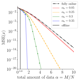
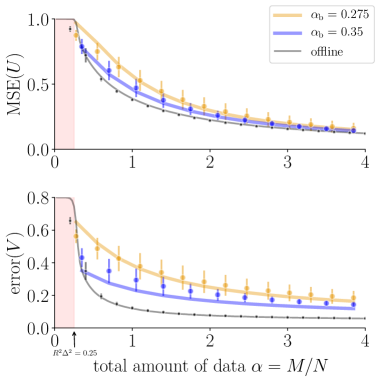
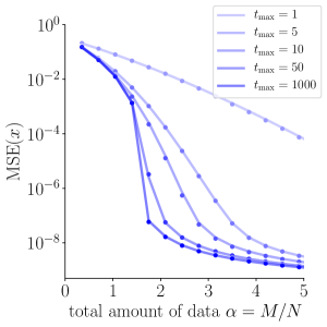
We now illustrate the above results on some examples. In Figure 1, we consider the SLR model and the perceptron with binary $\pm 1$ parameters, both with random matrices $\Phi\in\mathbb{R}^{M\times N}$, $\Phi_{\mu i}\sim\mathcal{N}(0,1/N)$. Our analysis quantifies the loss coming from using mini-batches with respect to a fully offline implementation. In the limit of small mini-batch $\alpha_{\text{b}}\to 0$, we recover the results of the ADF algorithm which performs fully online learning, processing one sample at a time [9, 11]. This suggests that the state evolution accurately describes the behavior of Mini-AMP beyond the theoretical assumption of $\alpha_{b}\!=\!O(1)$, even for mini-batches as small as a single sample.

The effect of the mini-batch sizes varies greatly with the problem. For the perceptron with $\pm 1$ weights, a zero error is eventually obtained after a sufficient number of mini-batches have been processed. Moreover, the dependence on the mini-batch size is mild: while the offline scheme achieves zero error at $\alpha\approx 1.5$ [27, 28], the fully online does it at $\alpha\approx 4.4$ [9], that is, going from offline to a fully online scheme costs only about three times more data points. The behavior of the Mini-AMP for SLR shows instead rather drastic changes with the mini-batch size. The MSE decays smoothly when the mini-batch size is small. However, as we increase it, a sudden decay occurs after a few mini-batches have been processed. For the noiseless case ($\Delta=0$), the study of the state evolution shows that the asymptotic (in $\alpha$) MSE is given by

$$\operatorname{MSE}_{x}(\alpha)\sim e^{-\frac{1}{\alpha_{\text{b}}}\log(1-\frac{\alpha_{\text{b}}}{\rho})\,\alpha},$$ (18)

if $\alpha_{\text{b}}\leq\rho$, and by 0 otherwise. These results provide a basis for an optimal choice of mini-batch size. Given the drastic change in behavior past a certain mini-batch size, one concludes that small investments in memory might be worthwhile, since they can lead to large gains in performance.

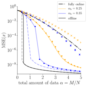
Finally, we have compared the Mini-AMP scheme with the streaming VB approach [12] using the mean-field algorithm described in [38] for SLR. While the mean-field approach is found to give results comparable to AMP in the offline case in [38], we see here that the results are considerably worse in the streaming problem. In fact, as shown in Figure 1 (center), mean-field can give worse performance than the fully online ADF, even when processing rather large mini-batches.

5.2 Phase transitions

Figure 2: Phase transitions in streaming SLR. Left: evolution of the mutual information in the streaming SLR problem as each mini-batch is processed. Parameters are set to $\rho=0.3$, $\Delta=10^{-8}$ and $\alpha_{\text{b}}=0.35$. Right: MSE of Mini-AMP for different mini-batch sizes. Mini-AMP achieves the MMSE for $\alpha_{b}<\rho$. For $\alpha_{b}>\rho$ the MMSE is zero after processing a single batch, while for batch sizes between $\rho<\alpha_{b}<0.49$ the Mini-AMP is suboptimal unless a sufficient number of mini-batches is processed.

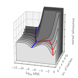
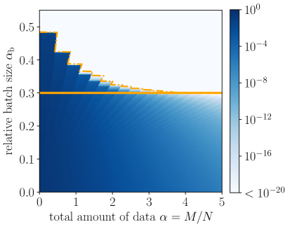
It turns out that, just as for the offline setting, there are phase transitions appearing for mini-batch learning, in terms of the learning error that is achievable information-theoretically (MMSE) or computationally efficiently (by Mini-AMP). These can be understood by an analysis of the function $i^{b}_{\rm RS}$, since the minimum of $i^{b}_{\rm RS}$ gives the MMSE, and since AMP is effectively trying to minimize $i^{b}_{\rm RS}$ starting from the MSE reached at the previous mini-batch steps.

Let us illustrate the reason behind the sharp phenomenon in the behavior of AMP in Fig.1. We show, in Fig. 2 (left), an example of the function $i^{b}_{\rm RS}({\cal E})$ for the streaming SLR problem as a function of the MSE ${\cal E}$ as each mini-batch is being processed. Initially, it presents a “good” and a “bad” minimum, at small and large MSEs respectively. In the very first batch, AMP reaches the bad minimum. As more batches are processed, the good minimum becomes global, but AMP is yet not able to reach it, and keeps returning the bad one instead. This indicates a computational phase transition, and we expect that other algorithms will, as AMP, fail to deliver the MMSE in polynomial time when this happens. Eventually, the good minimum becomes unique, at which point AMP is able to reach it, thus yielding the sudden decay observed in Figure 1.

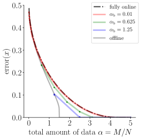
Consider now the Bayes-optimal "streaming-MMSE" given by the global minimum of the mutual information at each step, regardless of whether AMP achieves it. In the offline noiseless case, the MMSE is achieved by AMP only if the processed batch has size $\alpha\geq\alpha_{\rm offline}$ or $\alpha\leq\rho$ [18]. In the streaming case, we also observe that Mini-AMP reaches the streaming-MMSE if the mini-batch size is sufficiently small or sufficiently large. In Figure 2 (right) we compare MMSE to the MSE reached by Mini-AMP, with a region between the full and dashed line where the algorithm is sub-optimal.

6 Mini-AMP for matrix factorization problems

​

Figure 3: Clustering with Mini-AMP on synthetic Gaussian mixture data (left) and real-world data (right). Left: mean-squared error in $U$ (centroids) and 0-1 loss in $V$ (labels) using different batch sizes. Solid lines give state evolution and symbols give averages over 100 instances of size $N=1000$. A transition at $\alpha_{\text{c}}=R^{2}\Delta^{2}=0.25$ prevents Mini-AMP from giving non-zero overlap when $\alpha_{\text{b}}<\alpha_{\text{c}}$. Parameters are set to $R=5$, $\Delta=0.1$. Right: clustering on MNIST and the 20 newsgroups dataset using Mini-AMP for model (19), with the prior on $U$ replaced with a non-negative Gaussian of mean zero and variance $0.1$, and the noise variance $\Delta$ estimated from the data. On MNIST, digits of size $N=784$ were clustered on $K=3$ classes (0, 1 and 2), whereas for the 20 newsgroups dataset, frequency statistics of $N=1000$ words and $K=3$ top-level hierarchies (comp, rec, and sci) were used. Batch sizes were set so that $\alpha_{b}=0.05$. Blue/red circles give the cumulative performance of Mini-AMP and mini-batch K-means [39], respectively, averaged over a 100 different orders of presentation. For the newsgroups dataset, a 2nd pass over the data was performed so that all labels could be recomputed with accurate estimation of the centroids; results of 1st and 2nd passes are shown in light/dark lines respectively.

We now consider the case of low-rank matrix factorization, and in particular clustering using the Gaussian mixture model (GMM) with $R$ clusters. For such problems, the generative model reads

$$P(U,V,Y)=\prod_{ij}\mathcal{N}(Y_{ij};\bm{U}_{i}\cdot\bm{V}_{j},\Delta)\prod_{i=1}^{N}\mathcal{N}(\bm{U}_{i};\bm{0},\mathbb{I}_{R})\prod_{j=1}^{M}\frac{1}{R}\sum_{k=1}^{R}\delta(\bm{V}_{j}-\mathbbm{e}_{k}),$$ (19)

where $\bm{U}_{i}$ and $\bm{V}_{j}$ give the $i$-th row of $U$ and $j$-th row of $V$ respectively. Each of the $R$ columns of $U$ describe the mean of a $N$-variate i.i.d. Gaussian, and $V$ has the role of picking one of these Gaussians. Finally, each column of $Y$ is given by the chosen column of $U$ plus Gaussian noise. In clustering, these are the data points, and the objective is to figure out the position of the centroids as well as the label assignment, given by the columns of $U$ and the rows of $V$ respectively. In the streaming setting the columns of the matrix $Y$ are arriving in mini-batches. The offline AMP algorithm, its state evolution, and corresponding proofs are known for matrix factorization from [17, 40, 19, 37, 23, 26]. The Mini-AMP is obtained by adjusting the update of the estimators using (12).

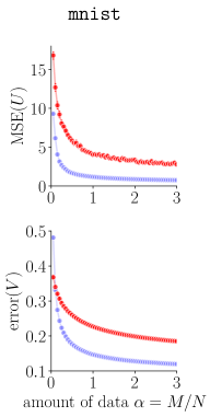
In GMM clustering with prior on U having zero mean, there is an interesting "undetectability" phase transition for $R\leq 4$. If the number of samples is such that $\alpha=M/N<\alpha_{c}=R^{2}\Delta^{2}$, then the Bayes optimal posterior asymptotically does not contain any information about the ground truth parameters [19]. This transition survives even when $R>4$, in the sense that AMP and other tractable algorithms are unable to find any information on the ground truth parameters.

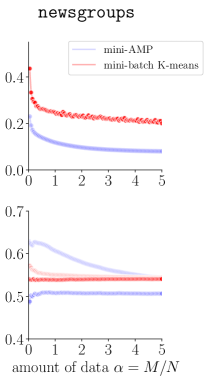
In the streaming problem, this undetectability implies that for mini-batches of relative size $\alpha_{\text{b}}<\alpha_{\text{c}}$, Mini-AMP does not improve the error of the random estimator, no matter the number of mini-batches presented. In particular, the fully online algorithm does not provide any useful output in this scenario. If $\alpha_{\text{b}}>\alpha_{\text{c}}$, on the other hand, an accurate reconstruction of the unknown values becomes possible. We illustrate the MSE as a function of the mini-batch size in Figure 3.

While we have presented Mini-AMP as a means for a theoretical analysis, it can be applied to real data, performing concrete learning tasks. To illustrate its efficacy, we have considered the classical problem of unsupervised clustering using the GMM. In Figure 3, Mini-AMP is shown to obtain better performance for real data clustering than mini-batch K-means, a state-of-the-art algorithm for streaming clustering [39].

7 Conclusion

Let us conclude by stating that the Mini-AMP algorithm can be applied to any problem for which the streaming can be defined and for which offline AMP exists. Therefore, we expect that this novel development will improve the usefulness of AMP algorithms in more practical situations.

Appendix A AMP equations for different classes of models

We present here the AMP equations for different models. As before, adapting them to the streaming setting is done by introducing $\bm{\Lambda}$, $\bm{\Theta}$ variables and replacing the $\eta(A,B)$ function with (12).

A.1 Generalized linear models

Denote by $\bm{y}\in\mathbb{R}^{M}$ the response variable, by $\Phi\in\mathbb{R}^{M\times N}$ the design matrix, and by $\bm{x}\in\mathbb{R}^{N}$ the parameter vector that we want to estimate. Then our generative model reads

$$P(\bm{y},\bm{x}|\Phi)=\prod_{\mu=1}^{M}P(y_{\mu}|z_{\mu}\equiv\bm{\Phi}_{\mu}\cdot\bm{x})\,\prod_{i=1}^{N}P_{X}(x_{i}).$$ (20)

The GAMP algorithm provides the following approximation to the marginals of $\bm{x}$

$$q_{x}(x_{i}|A_{i},B_{i})=\frac{1}{Z_{x}(A_{i},B_{i})}\,P_{X}(x_{i})\,e^{-\frac{1}{2}A_{i}x_{i}^{2}+B_{i}x_{i}},$$ (21)

and, to the marginals of $\bm{z}$

$$q_{z}(z_{\mu}|y_{\mu},\omega_{\mu},V_{\mu})=\frac{1}{Z_{z}(y_{\mu},\omega_{\mu},V_{\mu})}\,P(y_{\mu}|z_{\mu})\,\frac{e^{-\frac{(z_{\mu}-\omega_{\mu})}{V_{\mu}}}}{\sqrt{2\pi V_{\mu}}}.$$ (22)

The parameters $\bm{A}$, $\bm{B}$, $\bm{\omega}$ and $\bm{V}$ are determined by iterating the GAMP equations. We denote the mean and variance of $q_{x}(A,B)$ by $\eta(A,B)=\frac{\partial}{\partial B}\log Z_{x}(A,B)$ and $\eta^{\prime}(A,B)=\frac{\partial\eta}{\partial B}(A,B)$ respectively; moreover, we define $g_{\text{out}}(y,\omega,V)=\frac{\partial}{\partial\omega}\log Z_{z}(y,\omega,V)$. The GAMP equations then read [14, 15]

$$\bm{\omega}^{(t)}=\Phi\hat{\bm{x}}^{(t)}-\bm{V}^{(t)}\circ\bm{g}^{(t-1)}, \bm{V}^{(t)}=(\Phi\circ\Phi)\,\hat{\bm{\sigma}}^{(t)},$$ (23)

$$g_{\mu}^{(t)}=g_{\text{out}}(y_{\mu},\omega_{\mu}^{(t)},V_{\mu}^{(t)})\;\forall\mu, \partial_{\omega}g_{\mu}^{(t)}=\partial_{\omega}g_{\text{out}}(y_{\mu},\omega_{\mu}^{(t)},V_{\mu}^{(t)})\;\forall\mu,$$

$$\bm{B}^{(t)}=\Phi^{T}\bm{g}^{(t)}+\bm{A}^{(t)}\circ\hat{\bm{x}}^{(t)}, \bm{A}^{(t)}=-(\Phi\circ\Phi)^{T}\,\partial_{\omega}\bm{g}^{(t)},$$

$$\hat{x}_{i}^{(t+1)}=\eta(A_{i}^{(t)},B_{i}^{(t)})\;\forall i, \hat{\sigma}_{i}^{(t+1)}=\eta^{\prime}(A_{i}^{(t)},B_{i}^{(t)})\;\forall i.$$

Note that, for a Gaussian likelihood $P(y|z)=\mathcal{N}(y;z,\Delta)$, $g_{\text{out}}(y,\omega,V)=\frac{y-\omega}{\Delta+V}$. Then, by defining $\bm{\tilde{z}}^{(t)}=\bm{y}-\bm{\omega}^{(t)}$ and replacing $\bm{V}^{(t)}$ and $\bm{A}^{(t)}$ by its averages, we get via the central limit theorem

$$V^{(t)}\approx\frac{1}{N}\sum_{i=1}^{N}\sigma^{(t)}(A^{(t)},B_{i}^{(t)}),\qquad A^{(t)}\approx\frac{\alpha}{\Delta+V^{(t)}},$$ (24)

where we have assumed the $\Phi_{\mu i}$ are i.i.d. and have zero mean and variance $1/N$. From these (5)-(7) follow through.

A.1.1 Variational Bayes

We compare AMP equations to the Variational Bayes (VB) ones, which we use with the Streaming Variational Bayes scheme. For simplicity we restrict ourselves to the Gaussian case. As usual, VB is derived by determining the $q_{i}(x_{i})$ which minimize

$$KL[{\textstyle\prod_{i}}q_{i}(x_{i})\|P(\bm{x}|\Phi,\bm{y})]=-\mathbb{E}_{\{q_{i}\}}\log P(\bm{y}|\Phi,\bm{x})+\sum_{i=1}^{N}\operatorname{KL}[q_{i}(x_{i})\|P_{X}(x_{i})]-\log P(\bm{y}|\Phi)$$ (25)

If done by means of a fixed-point iteration, this minimization leads to [38]

$$\hat{x}_{i}^{(t+1)}=\eta\bigg{(}\frac{1}{\Delta}\sum_{\mu}\Phi_{\mu i}^{2},\frac{1}{\Delta}\sum_{\mu}\Phi_{\mu i}(y_{\mu}-{\textstyle\sum_{j\neq i}}\Phi_{\mu j}\hat{x}_{j}^{(t)})\bigg{)}\;\forall i,$$ (26)

where $\eta$ is defined as before. A closer inspection shows that the same equations are obtained by setting $\bm{V}^{(t)}=0$ in (23).

As shown in [38], this iteration leads to good results when performed sequentially, if the noise $\Delta$ is not fixed but learned. We employ this same strategy in our experiments.

A.1.2 Assumed Density Filtering

The assumed density filtering (ADF) algorithm [3, 4] replaces the posterior at each step $k$, $P(\bm{x}|\bm{\Phi}_{k},y_{k})\propto P(y_{k}|\bm{\Phi}_{k},\bm{x})\,Q_{k-1}(\bm{x})$, by the distribution $Q_{k}(\bm{x})$ that minimizes

$$\operatorname{KL}[P(\bm{x}|\bm{\Phi}_{k},y_{k})\|Q_{k}(\bm{x})].$$ (27)

Note this is the direct KL divergence, and not the reverse one $\operatorname{KL}[Q(\bm{x})\|P(\bm{x}|\Phi,\bm{y})]$ that is minimized in Variational Bayes. In particular if $Q_{k}(\bm{x})=\prod_{i=1}^{N}q_{k}(x_{i})$, then minimizing this KL divergence leads to the following integral

$$q_{k}(x_{i})=q_{k-1}(x_{i})\int\bigg{[}\prod_{j\neq i}dx_{j}\,q_{k-1}(x_{j})\bigg{]}\,P(y_{k}|\bm{\Phi}_{k},\bm{x})\;\forall i,$$ (28)

which is tractable since we are processing a single sample $y_{k}$ at a time, i.e. since the likelihood consists of a single factor. These are actually the exact marginals of $P(\bm{x}|\bm{\Phi}_{k},y_{k})$, and also the equations given by the belief propagation (BP) algorithm in the single sample limit.

The ADF equations for GLMs can be derived by using (28) together with the central limit theorem [11]. Because BP gives ADF in the single sample limit, AMP (which is based on BP) gives the equations derived by [11] when $M=1$, if one additionally neglects the correction term $-\bm{V}^{(t)}\bm{g}^{(t-1)}$ (analogously, if a single iteration is performed).

Algorithm 2 Assumed Density Filtering for GLMs [11]

1:initialize $\Lambda_{0,i}=0$, $\Theta_{0,i}=0\;\forall i$

2:for $k\leftarrow 1$ to $M$ do

3:     compute $\omega_{k}=\bm{\Phi}_{k}\cdot\hat{\bm{x}}_{k-1}$, $V_{k}=(\bm{\Phi}_{k}\circ\bm{\Phi}_{k})\cdot\hat{\bm{\sigma}}_{k-1}$

4:     compute $g_{k},\partial_{\omega}g_{k}$ following (23)

5:     compute $\bm{A}_{k}$, $\bm{B}_{k}$ following (23)

6:     compute $\bm{\hat{\sigma}}_{k}$, $\hat{\bm{x}}_{k}$ following (12)

7:     accumulate $\bm{\Lambda}_{k}\leftarrow\bm{\Lambda}_{k-1}+\bm{A}_{k}$

8:     accumulate $\bm{\Theta}_{k}\leftarrow\bm{\Theta}_{k-1}+\bm{B}_{k}$

9:end for

A.2 Low-rank matrix factorization

Denote by $Y\in\mathbb{R}^{N\times M}$ the matrix we want to factorize, and by $U\in\mathbb{R}^{N\times R}$, $V\in\mathbb{R}^{M\times R}$ the matrices which product approximates $Y$. The generative model then reads

$$P(Y,U,V)=\prod_{ij}P(Y_{ij}|W_{ij}\equiv\bm{U}_{i}\cdot\bm{V}_{j})\,\prod_{i=1}^{N}P_{U}(\bm{U}_{i})\,\prod_{j=1}^{M}P_{V}(\bm{V}_{j}),$$ (29)

where $\bm{U}_{i}$ and $\bm{V}_{j}$ denote the $i$-th and $j$-th rows of $U$ and $V$ respectively. The algorithm provides the following approximation to the marginal of $\bm{U}_{i}$

$$q_{U}(\bm{U}_{i}|A_{U},\bm{B}_{U,i})=\frac{1}{Z_{U}(A_{U},\bm{B}_{U,i})}\,P_{U}(\bm{U}_{i})\,e^{-\frac{1}{2}\bm{U}_{i}^{T}A_{U}\bm{U}_{i}+\bm{B}_{U,i}^{T}\bm{U}_{i}}.$$ (30)

and $q_{V}$ is analogously defined as the marginal of $\bm{V}_{j}$. As in the previous case, $A_{U}\in\mathbb{R}^{R\times R}$ and $\bm{B}_{U,i}\in\mathbb{R}^{R}$ are to be determined by iterating a set of equations. We denote by $B_{U}$ the $N\times R$ matrix which rows are given by $\bm{B}_{U,i}$, $i=1,\dots,N$. The functions $\eta_{U}(A,\bm{B})=\mathbb{E}_{q_{U}}\,\bm{U}=\nabla_{\bm{B}}\log Z_{U}(A,\bm{B})$ and $\eta^{\prime}_{U}(A,\bm{B})=\nabla_{\bm{B}}\eta_{U}(A,\bm{B})$ give the mean and covariance of $q_{U}$, and $\eta_{V}$ and $\eta^{\prime}_{V}$, defined analogously, the mean and covariance of $q_{V}$.

In order to write the AMP equations, we first introduce

$$J_{ij} =\frac{1}{\sqrt{N}}\frac{\partial\ln P(Y_{ij}|w=0)}{\partial w},$$ (31)

$$\beta =\frac{1}{N}\,\mathbb{E}_{P(y|w=0)}\bigg{[}\frac{\partial\ln P(y|w=0)}{\partial w}\bigg{]}^{2}.$$

so as to define an effective Gaussian channel [41]. The equations to be iterated are then

$$B_{U}^{(t)}=J\hat{V}^{(t)}-\beta\Sigma_{V}^{(t)}\hat{U}^{(t-1)}, A_{U}^{(t)}=\beta\,\hat{V}^{(t)}\hat{V}^{{(t)}^{T}},$$ (32)

$$\hat{\bm{U}}_{i}^{(t)}=\eta(A_{U}^{(t)},\bm{B}_{U,i}^{(t)})\;\forall i, \Sigma_{U}^{(t)}=\sum_{i=1}^{N}\eta^{\prime}(A_{U}^{(t)},\bm{B}_{U,i}^{(t)}),$$

$$B_{V}^{(t)}=J^{T}\hat{U}^{(t)}-\beta\Sigma_{U}^{(t)}\hat{V}^{(t)}, A_{V}^{(t)}=\beta\,\hat{U}^{(t)}\hat{U}^{{(t)}^{T}},$$

$$\hat{\bm{V}}_{j}^{(t+1)}=\eta(A_{V}^{(t)},\bm{B}_{V,j}^{(t)})\;\forall j, \Sigma_{V}^{(t+1)}=\sum_{j=1}^{M}\eta^{\prime}(A_{V}^{(t)},\bm{B}_{V,j}^{(t)}).$$

In order to adapt this algorithm to the online setting, we repeat procedure (12) and, as the $k$-th batch is processed, replace calls to $\eta_{U}(A_{U},\bm{B}_{U})$ by

$$\eta_{U}\Bigg{(}\underbrace{\sum_{\ell=1}^{k-1}A_{U,\ell}}_{\Lambda_{k-1}}+A_{U,k}^{(t)},\underbrace{\sum_{\ell=1}^{k-1}\bm{B}_{U,\ell}}_{\bm{\Theta}_{k,i}}+\bm{B}_{U,k}^{(t)}\Bigg{)}.$$ (33)

We assume that $U$ is fixed and $V_{k}$ changes for each batch $k$; thus, the calls to $\eta_{V}$ do not change.

Appendix B State evolution and asymptotic limits

Through the state evolution equations, we analyze the behaviour and performance of the algorithms described in the previous section. We restrict ourselves to the Bayes-optimal case (i.e. the Nishimori line), where the generative model is known. The strategy we use to go from the offline to the streaming setting is easily adapted to the non-optimal case.

B.1 Generalized linear models

The state evolution equations for a GLM with likelihood $P(y|z)$ and prior $P_{X}(x)$ are

$$\left\{\begin{aligned} &\hat{m}^{(t)}=-\alpha\,\mathbb{E}_{y,z,w}\;\partial_{w}g(y,w,\rho-m^{(t)}),\\ &m^{(t+1)}=\mathbb{E}_{x,b}\;x\eta(\hat{m}^{(t)},b),\end{aligned}\right.$$ (34)

where we denote $\rho=\mathbb{E}x^{2}$, and the averages are taken with respect to $P(x,b)=P_{X}(x)\mathcal{N}(b;\hat{m}x,\hat{m})$ and $P(y,\omega,z)=P(y|z)\mathcal{N}(z;\omega,\rho-m)\mathcal{N}(\omega;0,m)$. The MSE at each step is obtained from ${\cal E}^{(t)}=\rho-m^{(t)}$. For a Gaussian likelihood $P(y|z)=\mathcal{N}(y;z,\Delta)$, $\hat{m}^{(t)}=\frac{\alpha}{\Delta+{\cal E}^{(t)}}$ and we recover (9).

The fixed points of the state evolution extremize the so-called replica free energy

$$\phi(m,\hat{m})=\frac{1}{2}m\hat{m}-\mathbb{E}_{b,x}\log Z_{x}(\hat{m},b)-\alpha\mathbb{E}_{y,\omega,z}\log Z_{z}(y,\omega,\rho-m)$$ (35)

which gives the large system limit of the Bethe free energy (extremized by AMP). The mutual information (10) differs from $\phi(m)=\operatorname*{extr}_{\hat{m}}\,\phi(m,\hat{m})$ by a constant – more specifically, by the entropy of $P(y|z)$, $i_{\text{RS}}(m)=\phi(m)-\alpha H[P(y|z)]$. For a Gaussian likelihood, $H[P(y|z)]=\frac{1}{2}\log(2\pi e\Delta)$.

In order to adapt this to the streaming setting, we introduce $\lambda_{k}^{(t)}=\sum_{\ell=1}^{k-1}\hat{m}_{\ell}^{(t_{\text{max}})}+\hat{m}_{k}^{(t)}$ and iterate instead, for each mini-batch $k$

$$\left\{\begin{aligned} &\lambda_{k}^{(t)}=\lambda_{k-1}-\alpha_{b}\,\mathbb{E}_{y,z,w}\;\partial_{w}g(y,w,\rho-m_{k}^{(t)}),\\ &m_{k}^{(t+1)}=\mathbb{E}_{x,b_{k}}\;x\eta(\lambda_{k}^{(t)},b),\end{aligned}\right.$$ (36)

with the averages now computed over $P(x,b_{k})=P_{X}(x)\mathcal{N}(b_{k};\lambda_{k}x,\lambda_{k})$. These equations should be iterated for $t=1,\dots,t_{\text{max}}$, at which point we assign $\lambda_{k}=\lambda_{k-1}^{(t_{\text{max}})}$. The MSE on $\bm{x}$ after mini-batch $k$ is processed is then given by ${\cal E}_{k}=\rho-m_{k}^{(t_{\text{max}})}$.

Note that in the small batch size limit ($\alpha_{b}\to 0$), the equation for $\lambda$ becomes an ODE

$$\frac{d\lambda}{d\alpha}=-\mathbb{E}_{y,z,w}\;\partial_{w}g(y,w,\rho-m(\lambda)),$$ (37)

which describes the performance of the ADF algorithm [3, 11].

The free energy is also easily rewritten

$$\phi_{k}(m_{k},\hat{m}_{k};\lambda_{k-1})=\frac{1}{2}m_{k}\hat{m}_{k}-\mathbb{E}_{b,x}\log Z_{x}(\lambda_{k-1}+\hat{m}_{k},b)-\alpha_{b}\,\mathbb{E}_{y,\omega,z}\log Z_{z}(y,\omega,\rho-m_{k}),$$ (38)

or analogously, by working with $\lambda_{k}=\lambda_{k-1}+\hat{m}_{k}$ instead of $\hat{m}_{k}$

$$\phi_{k}(m_{k},\lambda_{k};\lambda_{k-1})=\frac{1}{2}m_{k}(\lambda_{k}-\lambda_{k-1})-\mathbb{E}_{b,x}\log Z_{x}(\lambda_{k},b)-\alpha_{b}\,\mathbb{E}_{y,\omega,z}\log Z_{z}(y,\omega,\rho-m_{k}).$$ (39)

from which it is clear that the extrema of $\phi_{k}$ are given by the fixed points of (36).

B.1.1 Asymptotic behavior

Equations (36) can be put in the following form

$$\left\{\begin{aligned} {\cal E}_{k}&=\varepsilon(\lambda_{k}),\\ \lambda_{k}&=\lambda_{k-1}+\alpha_{b}\,\delta({\cal E}_{k}),\end{aligned}\right.$$ (40)

where $\varepsilon(\lambda_{k})$ and $\delta({\cal E}_{k})$ are functions that depend on the prior/channel respectively. Assuming $\varepsilon$ is invertible, we rewrite this system of equations as a function of ${\cal E}_{k}$ only

$$\varepsilon^{-1}({\cal E}_{k})=\varepsilon^{-1}({\cal E}_{k-1})+\alpha_{b}\,\delta({\cal E}_{k}),$$ (41)

and then solve this equation for ${\cal E}_{k}$; that gives us a recurrence relation which is unsolvable in most cases. We use instead asymptotic forms for $\varepsilon$ and $\delta$, obtained in the $\lambda\to\infty$, ${\cal E}\to 0$ limit. For the Bernoulli-Gaussian prior $P_{0}(x_{i})=\rho\,\mathcal{N}(x_{i};0,1)+(1-\rho)\,\delta(x_{i})$, we have

$$\varepsilon(\lambda)\sim\frac{\rho}{\lambda},$$ (42)

while a Gaussian likelihood gives, in the $\Delta\to 0$ limit, $\delta({\cal E})=\frac{1}{{\cal E}}$. Thus, for SLR

$$\frac{\rho}{{\cal E}_{k}}\approx\frac{\rho}{{\cal E}_{k-1}}+\frac{\alpha_{\text{b}}}{{\cal E}_{k}}\;\Rightarrow\;{\cal E}_{k}\approx\bigg{(}1-\frac{\alpha_{b}}{\rho}\bigg{)}^{k}{\cal E}_{0},$$ (43)

leading to (18). In the $\alpha_{b}\to 0$ limit we recover the expression obtained by [11], $\operatorname{MSE}(\alpha)\sim e^{-\frac{\alpha}{\rho}}$.

B.2 Low-rank matrix factorization

Also for low-rank models the large $N$ limit can be analyzed by taking into account that $A_{U,V}^{(t)}$ and $B_{U,V}^{(t)}$ converge in distribution to [41]

$$A_{U}^{(t)} =\beta M_{V}^{(t)}, \;\bm{B}_{U} \sim\mathcal{N}(\beta M_{V}^{(t)}\bm{U},\beta M_{V}^{(t)}),$$ (44)

$$A_{V}^{(t)} =\beta M_{U}^{(t)}, \;\bm{B}_{V} \sim\mathcal{N}(\beta M_{U}^{(t)}\bm{V},\beta M_{U}^{(t)}),$$

where $M_{U},M_{V}\in\mathbb{R}^{R\times R}$ are the overlap matrices between the ground truth and the estimate at time $t$, that is

$$M_{U}^{(t)}=\mathbb{E}_{\bm{U},\bm{B}_{U}}\,\bm{U}^{T}\eta_{U}(\beta M_{V}^{(t)},\bm{B}_{U}),$$ (45)

$$M_{V}^{(t+1)}=\alpha\,\mathbb{E}_{\bm{V},\bm{B}_{V}}\,\bm{V}^{T}\eta_{V}(\beta M_{U}^{(t)},\bm{B}_{V}).$$

While computing the expectations might become unfeasible for $R>1$, an ansatz of the following form can often be used [41, 19]

$$M_{U,V}=a_{U,V}\mathbb{I}_{R}+b_{U,V}\mathbb{J}_{R},$$ (46)

with $\mathbb{J}_{R}$ denoting the $R\times R$ matrix of ones. This significantly simplifies the iteration above.

Again we adapt this to the online case by incrementing the matrices obtained as each batch is processed, that is, we replace $M_{V}$ by

$$\lambda_{V,k}^{(t+1)}=\lambda_{V,k-1}+\alpha_{b}\mathbb{E}_{\bm{V},\bm{B}_{V}}\,\bm{V}^{T}\eta_{V}(\beta M_{U,k}^{(t)},\bm{B}_{V}).$$ (47)

Note that since $U$ is fixed, the equation for $M_{U}$ does not change.

The replica free energy reads, in the offline case

$$\phi(M_{U},M_{V})=\frac{\beta}{2}\operatorname{Tr}M_{U}M_{V}^{T}\,-\mathbb{E}_{\bm{U},\bm{B}_{U}}\,\log Z_{U}(\beta M_{V},\bm{B}_{U})\,-\mathbb{E}_{\bm{V},\bm{B}_{V}}\,\log Z_{V}(\beta M_{U},\bm{B}_{V}),$$ (48)

and we adapt it to the online case by taking into account that $\lambda_{V}$ is being incremented

$$\phi(M_{U,k},\lambda_{V,k} ;\lambda_{V,k-1})=\frac{\beta}{2}\operatorname{Tr}M_{U,k}\,(\lambda_{V,k}-\lambda_{V,k-1})\,-$$ (49)

$$\mathbb{E}_{\bm{U},\bm{B}_{U}}\,\log Z_{U}(\beta\lambda_{V,k},\bm{B}_{U})\,-\mathbb{E}_{\bm{V},\bm{B}_{V}}\,\log Z_{V}(\beta M_{U,k},\bm{B}_{V}).$$

Appendix C Performance for different number of iterations

For our experiments in Figure 1, Mini-AMP has been iterated until, for each block, convergence is achieved – that is, until $\frac{1}{N}\|\hat{\bm{x}}^{(t)}-\hat{\bm{x}}^{(t-1)}\|_{1}<10^{-13}$. Remarkably, our framework allows us to study the performance of the algorithm even if we do not iterate it until convergence, but only for a few steps $t_{\text{max}}$ instead. In Figure 4, we investigate the performance of Mini-AMP under the same settings of Figure 1 (center), for different values of $t_{\text{max}}$. We observe that the performance deteriorates if convergence is not reached.

Figure 4: Performance of the Mini-AMP algorithm for different values of $t_{\text{max}}$, under the same settings of Figure 1 (center), and $\alpha_{b}=0.35$. Solid lines give state evolution, and symbols results of empirical experiments averaged over 10 realizations of size $N=2000$. The performance deteriorates if the algorithm is not iterated until convergence.

Appendix D Experiments on real-world data

For the experiments with real data, we have used the following model

$$P(U,V,Y)=\prod_{ij}\mathcal{N}(Y_{ij};\bm{U}_{i}\cdot\bm{V}_{j},\Delta)\prod_{i=1}^{N}\mathcal{N}_{\geq 0}(\bm{U}_{i};\bm{0},\sigma^{2}\mathbb{I}_{R})\prod_{j=1}^{M}\frac{1}{R}\sum_{k=1}^{R}\delta(\bm{V}_{j}-\mathbbm{e}_{k}),$$ (50)

where

$$\mathcal{N}_{\geq 0}(\bm{x};\bm{\mu},\sigma^{2}\mathbb{I}_{R})=\frac{1}{\mathcal{Z}(\bm{\mu},\sigma^{2})}\,\mathcal{N}(\bm{x};\bm{\mu},\sigma^{2}\mathbb{I}_{R})\,\prod_{k=1}^{R}\theta(x_{k})$$ (51)

is a truncated normal distribution supported on the positive quadrant of a $R$-dimensional space, and $\mathcal{Z}(\bm{\mu},\sigma^{2})$ ensures proper normalization.

Note that evaluating the $\eta(A,\bm{B})$ function in this case is not trivial, since it depends on the following integral

$$Z_{U}(A,\bm{B}) =\frac{1}{\mathcal{Z}(\bm{\mu},\sigma^{2})}\,\int d\bm{x}\,e^{-\frac{1}{2}\bm{x}^{T}A\bm{x}+\bm{B}^{T}\bm{x}}\,\prod_{k=1}^{R}P_{0}(x_{k})$$ (52)

$$\propto\int\prod_{k=1}^{R}dx_{k}\,P_{0}(x_{k})\,e^{-\frac{1}{2}A_{kk}x_{k}^{2}+\big{(}B_{k}+\sum_{\ell\neq k}A_{k\ell}x_{\ell}\big{)}x_{k}}$$

where, in this case, $P_{0}(x_{k})=\mathcal{N}(x_{k};\mu_{k},\sigma^{2})\,\theta(x_{k})$. We proceed by performing a mean-field approximation. We first define

$$\tilde{\eta}(A,B)=\frac{\partial}{\partial B}\log\int dx\,P_{0}(x)\,e^{-\frac{1}{2}Ax^{2}+Bx}.$$ (53)

for scalar $A$ and $B$. Then, for each $i=1,\dots,N$, we iterate

$$\hat{U}_{ik}=\tilde{\eta}\big{(}A_{kk},B_{ik}-\frac{1}{2}\sum_{\ell\neq k}A_{k\ell}\hat{U}_{i\ell}\big{)}$$ (54)

sequentially in $k=1,\dots,R$ until convergence is reached, at which point we use the values obtained for assigning $\bm{\hat{U}}^{(t)}$ in AMP. The variances are computed from

$$\tilde{\sigma}_{ik}=\tilde{\eta}^{\prime}\big{(}A_{kk},B_{ik}-\frac{1}{2}\sum_{\ell\neq k}A_{k\ell}\hat{U}_{i\ell}\big{)}$$ (55)

and the covariance matrix used in AMP is obtained as a function of these variances

$$\sigma_{k\ell}=\left\{\begin{aligned} &\sum_{i=1}^{N}\tilde{\sigma}_{ik},\quad&&\text{if $k=\ell$},\\ &-\frac{1}{2}A_{k\ell}\sum_{i=1}^{N}\tilde{\sigma}_{ik}\tilde{\sigma}_{i\ell},\quad&&\text{otherwise},\end{aligned}\right.$$ (56)

where in order to assign the off-diagonal terms we have used a linear response approximation, $\sigma_{k\ell}=\sum_{i=1}^{N}\frac{\partial\hat{U}_{ik}}{\partial B_{i\ell}}$.

We proceed by detailing other aspects of the experiments

Initialization

At the first few mini-batches (usually the first five), we reinitialize the position of the centroids. We use the same strategy as the k-means++ algorithm [42]: the first centroid is picked at random from the data points, and the next ones are sampled so as to have them far apart from each other. The labels are initialized according to the closest centroid.

Stopping criterion

For each batch, Mini-AMP was iterated either for 50 steps or until $\frac{1}{NR}\sum_{ik}|\hat{U}_{ik}^{(t)}-\hat{U}_{ik}^{(t-1)}|+\frac{1}{MR}\sum_{jk}|\hat{V}_{jk}^{(t)}-\hat{V}_{jk}^{(t-1)}|<10^{-7}$.

Noise learning

We do not assign a fixed value for $\Delta$, but instead update it after each mini-batch is processed using a simple learning rule

$$\hat{\Delta}_{k}=\frac{1}{NM}\sum_{ij}(Y_{k,ij}-\bm{\hat{U}}_{k,i}\cdot\bm{V}_{k,j})^{2}.$$ (57)

Preprocessing

For MNIST, we work with all samples of digits 0, 1 and 2. They are rescaled so that the pixel intensities are between 0 and 1. For the 20 newsgroups dataset, we build Term Frequency Inverse Document Frequency (TF-IDF) features for 3 top-level hierarchies (comp, rec and sci), and use the 1000 most frequent words; we rescale each feature vector so that its maximum is equal to 1.

Mini-batch K-means

We use the mini-batch K-means [39] implementation available on scikit-learn [43]. Default parameters were used, apart from the centroids initialization, which was set to random normal variables of zero mean and variance $10^{-3}$ – this seemed to improve the algorithm performance with respect to the standard choices.

References

- Bottou [2010] L. Bottou. Large-scale machine learning with stochastic gradient descent. In Proc. COMPSTAT, pages 177–186, 2010.
- Hoffman et al. [2013] M. D. Hoffman, D. M. Blei, C. Wang, and J. Paisley. Stochastic variational inference. J. Machine Learning Research, 14(1):1303–1347, 2013.
- Opper [1998] M. Opper. A Bayesian approach to online learning. In D. Saad, editor, On-line learning in Neural Networks, pages 363–378. Cambridge University Press, 1998.
- Minka [2001] T. P. Minka. Expectation propagation for approximate Bayesian inference. In Proc. Conf. on Uncertainty in Artificial Intelligence, pages 362–369, 2001.
- Mitliagkas et al. [2013] I. Mitliagkas, C. Caramanis, and P. Jain. Memory limited, streaming pca. In Adv. in Neural Info. Proc. Systems, 2013.
- Wang and Lu [2016] C. Wang and Y. M. Lu. Online learning for sparse PCA in high dimensions: Exact dynamics and phase transitions. In Proc. IEEE Info. Theory Workshop, pages 186–190, 2016.
- Kinouchi and Caticha [1992] O. Kinouchi and N. Caticha. Optimal generalization in perceptrons. Journal of Physics A, 25(23):6243, 1992.
- Biehl and Riegler [1994] M. Biehl and P. Riegler. On-line learning with a perceptron. EPL, 28(7):525, 1994.
- Solla and Winther [1998] S. Solla and O. Winther. Optimal perceptron learning: as online Bayesian approach. In D. Saad, editor, On-line Learning in Neural Networks, pages 379–398. Cambridge, 1998.
- Saad [1999] D. Saad. On-line learning in neural networks, volume 17. Cambridge, 1999.
- Rossi et al. [2016] P. V. Rossi, Y. Kabashima, and J. Inoue. Bayesian online compressed sensing. Phys. Rev. E, 94(2):022137, 2016.
- Broderick et al. [2013] T. Broderick, N. Boyd, A. Wibisono, A. C. Wilson, and M. I. Jordan. Streaming variational Bayes. In Adv. in Neural Info. Proc. Systems, pages 1727–1735, 2013.
- Donoho et al. [2009] D. L. Donoho, A. Maleki, and A. Montanari. Message-passing algorithms for compressed sensing. Proc. Nat. Acad. Sci., 106(45):18914–18919, 2009.
- Rangan [2011] S. Rangan. Generalized approximate message passing for estimation with random linear mixing. In Proc. IEEE Int. Symp. on Info. Theory, pages 2168–2172, 2011.
- Zdeborová and Krzakala [2016] L. Zdeborová and F. Krzakala. Statistical physics of inference: Thresholds and algorithms. Advances in Physics, 65(5):453–552, 2016.
- Mézard and Montanari [2009] M. Mézard and A. Montanari. Information, Physics, and Computation. Oxford, 2009.
- Rangan and Fletcher [2012] S. Rangan and A. K. Fletcher. Iterative estimation of constrained rank-one matrices in noise. In IEEE Int. Symp. on Info. Theory, pages 1246–1250, 2012.
- Krzakala et al. [2012] F. Krzakala, M. Mézard, F. Sausset, Y. Sun, and L. Zdeborová. Probabilistic reconstruction in compressed sensing: algorithms, phase diagrams, and threshold achieving matrices. J. of Statistical Mechanics: Theory and Experiment, (08):P08009, 2012.
- Lesieur et al. [2016] T. Lesieur, C. De Bacco, J. Banks, F. Krzakala, C. Moore, and L. Zdeborová. Phase transitions and optimal algorithms in high-dimensional Gaussian mixture clustering. Proc. Allerton Conf. on Comm., Control, and Computing, pages 601–608, 2016.
- Lesieur et al. [2017a] T. Lesieur, L. Miolane, M. Lelarge, F. Krzakala, and L. Zdeborová. Statistical and computational phase transitions in spiked tensor estimation. arXiv Preprint [math.ST]:1701.08010, 2017a.
- Bayati and Montanari [2011] M. Bayati and A. Montanari. The Dynamics of Message Passing on Dense Graphs, with Applications to Compressed Sensing. IEEE Trans. on Inf. Th., 57(2):764–785, February 2011.
- Bayati et al. [2015] M. Bayati, M. Lelarge, and A. Montanari. Universality in polytope phase transitions and message passing algorithms. Annals of Applied Probability, 25(2):753–822, 2015.
- Barbier et al. [2016] J. Barbier, M. Dia, N. Macris, F. Krzakala, T. Lesieur, and L. Zdeborová. Mutual information for symmetric rank-one matrix estimation: A proof of the replica formula. In Adv. in Neural Info. Proc. Systems, 2016.
- Barbier et al. [2017] J. Barbier, N. Macris, M. Dia, and F. Krzakala. Mutual information and optimality of approximate message-passing in random linear estimation. arXiv Preprint [cs.IT]:1701.05823, 2017.
- Reeves and Pfister [2016] G. Reeves and H. D. Pfister. The replica-symmetric prediction for compressed sensing with Gaussian matrices is exact. In IEEE Int. Symp. on Info. Theory, pages 665–669, 2016.
- Miolane [2017] L. Miolane. Fundamental limits of low-rank matrix estimation. arXiv Preprint [math.PR]:1702.00473, 2017.
- Gardner and Derrida [1989] E. Gardner and B. Derrida. Three unfinished works on the optimal storage capacity of networks. J. of Phys. A: Mathematical and General, 22(12):1983, 1989.
- Györgyi [1990] G. Györgyi. First-order transition to perfect generalization in a neural network with binary synapses. Phys. Rev. A, 41:7097–7100, 1990.
- Candès et al. [2006] E. J. Candès, J. K. Romberg, and T. Tao. Stable signal recovery from incomplete and inaccurate measurements. Communications on Pure and Applied Mathematics, 59(8):1207–1223, 2006.
- Rangan et al. [2016] S. Rangan, P. Schniter, and A. Fletcher. Vector approximate message passing. arXiv Preprint [cs.IT]:1601.03082, 2016.
- Çakmak et al. [2014] B. Çakmak, O. Winther, and B. H. Fleury. S-amp: Approximate message passing for general matrix ensembles. In IEEE Info. Theory Workshop, pages 192–196. IEEE, 2014.
- Gardner and Derrida [1988] E. Gardner and B. Derrida. Optimal storage properties of neural network models. J. of Phys. A: Mathematical and General, 21(1):271, 1988.
- Krzakala et al. [2016] F. Krzakala, J. Xu, and L. Zdeborová. Mutual information in rank-one matrix estimation. In IEEE Info. Theory Workshop, pages 71–75, 2016.
- Kabashima et al. [2016] Y. Kabashima, F. Krzakala, M. Mézard, A. Sakata, and L. Zdeborová. Phase transitions and sample complexity in bayes-optimal matrix factorization. IEEE Trans. on Info. Theory, 62:4228–4265, 2016.
- Talagrand [2003] M. Talagrand. Spin glasses: a challenge for mathematicians: cavity and mean field models, volume 46. Springer Science & Business Media, 2003.
- Lelarge and Miolane [2016] M. Lelarge and L. Miolane. Fundamental limits of symmetric low-rank matrix estimation. arXiv Preprint [math.PR]:1611.03888, 2016.
- Lesieur et al. [2017b] T. Lesieur, F. Krzakala, and L. Zdeborová. Constrained low-rank matrix estimation: Phase transitions, approximate message passing and applications. arXiv Preprint [math.ST]:1701.00858, 2017b.
- Krzakala et al. [2014] F. Krzakala, A. Manoel, E. W. Tramel, and L. Zdeborová. Variational free energies for compressed sensing. In IEEE Int. Symp. on Info. Theory, pages 1499–1503, 2014.
- Sculley [2010] D. Sculley. Web-scale k-means clustering. In Proc. Int. Conf. on World Wide Web, pages 1177–1178, 2010.
- Matsushita and Tanaka [2013] R. Matsushita and T. Tanaka. Low-rank matrix reconstruction and clustering via approximate message passing. In Adv. in Neural Info. Proc. Systems, 2013.
- Lesieur et al. [2015] T. Lesieur, F. Krzakala, and L. Zdeborová. MMSE of probabilistic low-rank matrix estimation: Universality with respect to the output channel. In Proc. Allerton Conf. on Communication, Control, and Computing, pages 680–687, 2015.
- Arthur and Vassilvitskii [2007] D. Arthur and S. Vassilvitskii. k-means++: The advantages of careful seeding. In Proceedings of the 18th Annual ACM-SIAM Symposium on Discrete Algorithms, pages 1027–1035. Society for Industrial and Applied Mathematics, 2007.
- Pedregosa et al. [2011] F. Pedregosa, G. Varoquaux, A. Gramfort, V. Michel, B. Thirion, O. Grisel, M. Blondel, P. Prettenhofer, R. Weiss, V. Dubourg, J. Vanderplas, A. Passos, D. Cournapeau, M. Brucher, M. Perrot, and E. Duchesnay. Scikit-learn: Machine learning in Python. Journal of Machine Learning Research, 12:2825–2830, 2011.