Dynamical typicality of embedded quantum systems

Abstract

We consider the dynamics of an arbitrary quantum system coupled to a large arbitrary and fully quantum mechanical environment through a random interaction. We establish analytically and check numerically the typicality of this dynamics, in other words the fact that the reduced density matrix of the system has a self-averaging property. This phenomenon, which lies in a generalized central limit theorem, justifies rigorously averaging procedures over certain classes of random interactions and can explain the absence of sensitivity to microscopic details of irreversible processes such as thermalisation. It provides more generally a new ergodic principle for embedded quantum systems.

Thermalisation is probably one of the most common phenomenon in nature. Its universality, i.e. the fact that it does not depend on microscopic details but only on a small set of macroscopic parameters (like temperature or pressure) has been known experimentally for a long time Carnot (1824); Boltzmann (1974). In typical conditions, non equilibrium dynamics is expected to lead to some stationary state, independent of initial conditions, where macroscopic quantities can be calculated using statistical thermodynamics Kubo et al. (1990); Landau and Lifschitz (1980); J. Gemmer (2004). Despite being broadly accepted, the foundations of this statistical framework are relying on a set of assumptions where the role of randomness and the associated lack of knowledge, the role of averaging over this randomness and the supposed link with temporal averages through ergodicity, are not justified in a satisfactory manner (see e.g. the discussion in Gemmer and Mahler (2003)).

On the various attempts for setting statistical mechanics on the firm ground of quantum theory, typicality statements are one of the most promising. They introduce some randomness in the problem and, relying on a key mathematical phenomenon: “measure concentration” Not ; Talagrand (1996), they show that surprisingly this randomness actually does not matter, as soon as the Hilbert space dimension of the system considered is large enough. Such randomness has been previously introduced on the choice of a global quantum statePopescu et al. (2006); Goldstein et al. (2006); Reimann (2007); Linden et al. (2009) (i.e. a state of a large closed system) and on the choice of the full HamiltonianvonNeumann (1929); Reimann (2016), in order to get respectively a local property, like the state of a subsystem, or some global property, like a macroscopic observable. The former approach, which provides “canonical typicality” is purely kinematic in the sense that it is fundamentally a consequence of the geometry of the space of states, and does not provide any dynamical information. On the other hand the later approach (called nowadays “normal typicality”, see Goldstein et al. (2010a, b)) is dynamical but by randomizing the full Hamiltonian, it does not allow to consider a specific system or environment.

In this Article, we consider the generic problem of a quantum system coupled to a quantum environment where we introduce randomness at the level of the interaction Hamiltonian only. By doing so we get dynamical results for several classes of interaction Hamiltonians and most importantly for arbitrary system, environment, and global initial state (i.e. of system and environment). We show that for almost all interaction Hamiltonians (in a sense to be defined hereafter) the reduced density matrix of the subsystem has a typical dynamics. In other words, the microscopic structure of interaction Hamiltonians does not matter and reduced density matrices have a self-averaging property at all times. These results have two important consequences: first they can explain the absence of sensitivity to microscopic details of processes like for instance thermalisation. Second they provide the rigorous ground for an averaging procedure over random interactions which can be used for analytical calculations performed with full generality i.e. for arbitrary system, environment, and initial state (see Ithier and Benaych-Georges for an application to the equilibrium state of an embedded quantum system). More generally, this work provide a rigorous justification for a new kind of ergodicity partly envisioned in the early work of Wigner and DysonDyson (1962) when modeling entire nuclear Hamiltonians using random matrices. Indeed, time averages or ensemble averages over states are not required anymore, the key concept is provided by an averaging procedure over the interaction Hamiltonian only.

Model.— We consider a system $S$ in contact with an environment $E$ and denote by $\mathcal{H}_{s}$, $\mathcal{H}_{e}$ their respective Hilbert spaces (see Fig.1). The composite system $S+E$ is a closed system whose Hilbert space is the tensor product $\mathcal{H}=\mathcal{H}_{s}\otimes\mathcal{H}_{e}$ and whose total Hamiltonian $\hat{H}$ is $\hat{H}=\hat{H}_{s}+\hat{H}_{e}+\hat{W}$ where $\hat{W}$ is an interaction term. The state of the composite system $S+E$ is described by a density matrix $\varrho(t)$ obeying the well-kown relation derived from the Schrödinger equation: $\varrho(\tau)=\hat{U}_{\tau}\varrho(0)\hat{U}_{\tau}^{\dagger}$ with $\hat{U}_{\tau}=e^{-i\hat{H}\tau}$ the evolution operator and $\tau=t/\hbar$. The initial state of $S+E$: $\rho(0)$, can be chosen arbitrarily. In particular it should be noted that the environment state can be pure, there is no requirement of thermal equilibrium in sharp contrast to most models of thermalisation and decoherenceWeiss (2012). As $S$ is not a closed system, its state is described by the reduced density matrix Landau (1927): $\varrho_{s}(\tau)=\operatorname{Tr}_{e}\varrho(\tau),$ where $\operatorname{Tr}_{e}$ denotes the partial trace with respect to the environment. The aim of this Letter is to characterize, in the limit of a large environment (i.e. $\dim\mathcal{H}_{e}\to\infty$), the behavior of $\varrho_{s}(\tau)$ considered as a function $f$ of the interaction $W$:

$$f(\hat{W})=\operatorname{Tr}_{e}\left(e^{-i\tau(H_{0}+W)}\varrho(0)e^{i\tau(H_{0}+W)}\right),$$

all other relevant parameters being fixed: $\tau$, initial state $\varrho(0)$, system Hamiltonian $\hat{H}_{s}$, environment density of states $\rho_{e}(\epsilon)$. For this purpose, we introduce deliberately some randomness in $\hat{W}$ by assuming a lack of knowledge on the microscopic details of $\hat{W}$ (i.e. the matrix elements of $\hat{W}$ themselves) compatible with some symmetry property (e.g. real or hermitian symmetry) and a macroscopic constraint (here the strength $\sigma_{w}^{2}=\operatorname{Tr}(\hat{W}.\hat{W}^{\dagger})/\dim\mathcal{H}$ is fixed). The main result of this paper shows that, surprisingly, the uncertainty on the $W_{n,m}$ does not preclude extracting useful information on the behavior of $f(\hat{W})=\varrho_{s}(\tau)$ for several classes of random interactions. Here, we will consider $W$ to be either a Wigner Band Random Matrix (WBRM i.e. of the type $W_{i,j}=a((i-j)/b)Y_{i,j}$ where $Y$ is a Wigner Random Matrix and $a(x)$ is a deterministic band profile, “b” being the bandwidth) or a Randomly Rotated Matrix (RRM i.e. of the type $U.D.U^{\dagger}$ with $D$ real diagonal fixed and $U$ unitary or orthogonal Haar distributed). In both cases, $W$ should be centered (i.e. $\operatorname{Tr}(W)=0$) and with fixed spectrum variance (i.e. $\operatorname{Tr}(\hat{W}.\hat{W}^{\dagger})/\dim\mathcal{H}=\sigma_{w}^{2}$ fixed). Such a choice for $\hat{W}$ is justified by the fact that the WBRM ensembles are attractive for modeling interactions in tight binding systems or generic conservative systems with complex behavior like heavy atoms and nuclei (see e.g. Flambaum et al. (1994); Fyodorov et al. (1996), references therein and the reviews in Weidenm ller and Mitchell (2009); Mitchell et al. (2010); Borgonovi et al. (2016)). Their band structure emerges from the finite energy range of interaction which can be seen as a consequence of some selection rules. On the other hand, matrices from the RRM ensembles are dense, which is a priori not compatible with a few body nature of interaction. Despite this, they can be useful for modelling local statistical properties of more physical Hamiltonians (seePorter (1965); Brody et al. (1981); Mehta (1991) and the discussion inBorgonovi et al. (2016)). At this stage, we provide analytical results on dynamical typicality for both these dense and sparse interaction matrix ensembles but it should be noted that our method could be used to study other ensembles.

Then we consider $f(W)=\varrho_{s}(t)$ and notice that such a function is defined on a high dimensional input space: the set of random interactions (dimension $\dim^{2}\mathcal{H}$) and takes values in a much lower dimension output space (since $\dim\mathcal{H}_{e}\gg 1$). In addition, as we will see in the following, the partial trace is balancing the dependence of $f(\hat{W})$ on all the $W_{n,m}$ (i.e. there is no outlier $\hat{W}_{n,m}$ on which $f$ depends mostly). As a consequence, the reduced density matrix will exhibit, for all random matrix ensembles considered before, a phenomenon known as the “concentration of measure”Talagrand (1996) that we shall describe now and quantify rigorously.

Concentration of measure.— Central Limit Theorems (CLTs) provide the simplest illustration of this phenomenon. Considering for instance an experiment whose measurement output $X$ is the subject of a random error, then averaging the outcomes of $N$ independent measurements $\{X_{1},...,X_{N}\}$ taken in stationary conditions will increase the signal over noise ratio typically by a factor $\sqrt{N}$ (i.e. $g(X_{1},...,X_{N})=1/N\sum_{k}X_{k}$ has a standard deviation $\sigma_{g}=\sigma_{X}/\sqrt{N}$). Surprisingly, the decrease of the relative fluctuations is not limited to the empirical average considered above but appears under very general assumptions on a function $g$ and the probability distribution $P$ of its input: this is the so-called “measure concentration” Talagrand (1996), a phenomenon envisioned in the early work of P. Lévy, but formally established by V. Milman and M. Gromov in the $1970$’s and the $1980$’s. It can be described informally as follows: a numerical function that depends in a regular way on many random independent variables, but not too much on any of them, is essentially constant and equal to its mean value almost everywhere. The simplest analytical tool to quantify this phenomenon (and the one we use here) is the Poincaré inequalityG. Anderson (2009): a Riemannian manifold $\Omega$ equipped with a probability measure $P$ is said to verify a Poincaré inequality if there exists $C>0$ such that for all functions $g:\Omega\rightarrow\mathbb{R}$ continuously differentiable, one has

$$\sigma_{g}^{2}=\operatorname{\mathbb{E}}[|g(X)-\operatorname{\mathbb{E}}[g]|^{2}]\leqslant\frac{1}{C}\operatorname{\mathbb{E}}[||\vec{\nabla}g||^{2}]$$ (1)

where

$$||\vec{\nabla}g||^{2}=\sum_{k}\left(\frac{\partial g}{\partial X_{k}}\right)^{2}$$

and where the average $\operatorname{\mathbb{E}}$ is relative to $P$. In other words, the variance of $g$ is controlled by the typical gradient strength over a constant $C$ (that we call the “Poincaré constant” in the following) usually related to the variance of the input. A first interesting case is when $C$ does not depend on the dimension and $||\nabla g||^{2}\approx 1/N$, e.g. with the empirical average case considered above where the central limit theorem provides an equality case: $g(X_{1},...,X_{N})=\frac{1}{N}\sum_{i}X_{i}$, the CLT provides $\sigma_{g}^{2}=\sigma_{X}^{2}/N$, since $||\nabla g||^{2}=1/N$ and $1/C=\sigma_{X}^{2}$. Another interesting case is when $1/C\approx 1/N$ and $||\nabla g||$ is upper bounded by a constant independent of the dimension, e.g. when $\Omega$ is the hypersphere $\mathbb{S}^{N}$ of radius $1$ of $\mathbb{R}^{N}$ (i.e. $\{X\in\mathbb{R}^{N}/||X||=1\}$) equipped with the Haar measure (i.e. the isotropic probability measure). In both cases, the relative fluctuations of $g$ around its mean value are ”squeezed” like $1/\sqrt{N}$ and the function is said to be concentrated around its mean, which is thus a very good estimate of $g$ at any point of the space of high dimensionality. Here, we consider the Poincaré inequality to be sufficient for our purpose, however it is possible to go beyond and characterize the statistics of $g$ in more detail (see e.g. Talagrand (1996); Milman and Schechtman (1986)).

Main result.— The set of Hermitian matrices we consider for $W$, when endowed with the probability measures we consider here (WBRM and RRM, see Supp. Mat. Sec. 2 for details) verify Poincaré inequalities with constants both lower bounded in the following way: $C\geq\frac{\dim\mathcal{H}_{s}\dim\mathcal{H}_{e}}{2\sigma_{\omega}^{2}}$ where $\sigma_{\omega}^{2}=\operatorname{Tr}(\hat{W}.\hat{W}^{\dagger})/\dim\mathcal{H}$. In addition, we provide in Supp. Mat. Sec.1 the following upper bound on the gradient of $f(W)=\varrho_{s}(t)$:

$$||\nabla_{W}\varrho_{s}||^{2}\leqslant 2\frac{t^{2}}{\hbar^{2}}\dim\mathcal{H}_{s}.$$ (2)

Using the Poincaré inequality in Eq.(1), we get the upper bound on the variance of the fluctuations of $\varrho_{s}$ away from its mean behavior :

$$\sigma_{\varrho}^{2}=\operatorname{\mathbb{E}}[||\varrho_{s}-\operatorname{\mathbb{E}}[\varrho_{s}]||^{2}]\leqslant\frac{4\sigma_{\omega}^{2}t^{2}}{\hbar^{2}}\frac{1}{\dim\mathcal{H}_{e}}$$ (3)

with $||A||^{2}=\operatorname{Tr}(A.A^{\dagger})$ and where $\operatorname{\mathbb{E}}$ is the average performed over the random matrix ensemble considered. One should note that there is a priori no genuine physical effect responsible for the dependence of the upper bound in Eq.(3) with time. This upper bound is not optimal but is sufficient to demonstrate typicality: for fixed values of $\sigma_{w}$ and $t$, one has $\sigma_{\varrho}\rightarrow 0$ when $\dim\mathcal{H}_{e}\to\infty$. The mesoscopic fluctuations of this function are decreasing down to zero as the dimension of the environment Hilbert space goes to infinity. We argue that this phenomenon is at the core of irreversible processes such as thermalisation: it is responsible for a self-averaging property of the reduced density matrix of $S$, considered as a function of the interaction Hamiltonian. This means that $\varrho_{s}(t)$ has a “typical” behavior for almost all interaction Hamiltonians within the classes considered. We have performed numerical simulations for a two level system coupled to a quantum environment (see Fig.1). For small $\dim\mathcal{H}_{e}$, we observe a random pattern (analogous to a “speckle” pattern in optics) for the probabilities of occupation of the states of $S$. This pattern can be seen as a signature of the microscopic structure of the interaction Hamiltonian. As $\dim\mathcal{H}_{e}$ is increased, the amplitude of the fluctuations of this “speckle” pattern decreases and a typical behavior (i.e. independent of the details of $\hat{W}$) emerges. To get an intuitive understanding of the concentration of measure phenomenon, it is worth comparing it to the Monte Carlo method for numerically estimating the integral of a function over some subspace. A good estimate of this integral is provided by a discrete average of the function sampled randomly over the subspace. Measure concentration provides a path along the opposite direction: one is interested in the value of a function at a single point of the subspace and in most cases, a very good estimate of this value is the average of the function over the subspace. As a consequence, it should be noted that this phenomenon provides an approximate way of calculation of $\varrho_{s}(t)$ simply by averaging: $\varrho_{s}(t)=\operatorname{Tr}_{e}(\varrho(t))\approx\mathbb{E}[\operatorname{Tr}_{e}(\varrho(t))]=\operatorname{Tr}_{e}\left(\operatorname{\mathbb{E}}[\varrho(t)]\right)$, where $\mathbb{E}$ is the average over the set of interaction Hamiltonians considered. This property will be used inIthier and Benaych-Georges in order to calculate analytically the equilibrium state of an embedded quantum system when thermalisation takes place. Finally, it is important to stress that the upper bound in Eq.(2) does not depend on the statistics of $\hat{W}$, meaning that our framework can be adapted straight away to other classes of random matrices as soon as a lower bound on $C$ is available for these classes. For instance, it would be very interesting to investigate embedded random matrix ensemblesFlambaum et al. (1996); Flambaum and Izrailev (2000); Kota (2014); Papenbrock and Weidenm ller (2007) which are relevant when enforcing a two body nature of the interaction.

Possible experimental test.— In order to test experimentally this dynamical typicality property, ultra cold atoms in optical lattices seem the most promisingBloch et al. (2012); Schreiber et al. (2015), since these systems provide now the best level of isolation from uncontrolled degrees of freedom, and as such, enforces the required global unitary evolution over a sufficient duration. Such systems allow an accurate and independent control of the relevant parameters of the Hamiltonian: one site interaction and inter-site hoping can be tuned conveniently by the lasers creating the lattice potentials and randomness can be inserted using optical speckle patterns. In addition, these systems provide local observable measurement, like for instance local atomic density measurement, and should allow to monitor the emergence of the predicted typical behavior as system size increases (i.e. the squeezing of the fluctuating pattern that we observe numerically on Fig.(1)).

Discussion and Summary.— Before summarize our results, it is interesting to put them into perspective by considering the motivations of the first users of random matrices in a physical context, Wigner and Dyson, who were studying the high energy neutron scattering spectra of medium and large weight nuclei (see for instance the reviews in Brody et al. (1981); Guhr et al. (1998); Weidenm ller and Mitchell (2009); Mitchell et al. (2010) in references therein). Facing the complexity of such spectra, Wigner renounces inferring the Hamiltonian of this complex $N$-body system from the experimental data and operates a drastic change of point of view. He assumes some statistical hypothesis on the entries of the Hamiltonian considered as a random matrix, which are compatible with the general symmetry properties associated with the integrals of motion. More precisely, the candidate nuclear Hamiltonian is written as a block-diagonal matrix where each block corresponds to given values of the “good” quantum numbers (i.e. the conserved quantities). The entries of each block are then assumed to be independent identically distributed random variables with variance and mean depending on the conserved quantities associated with the block considered. Then averaging over this ensemble of Hamiltonians, one gets typical properties and in particular the average behavior of energy levels which is of prime importance for nuclear reactions and can be compared to experimental data. As noticed by Metha Mehta (1991) and Dyson Dyson (1962), the approach of Wigner is much more radical than the standard statistical physics approach: there is a subjective lack of knowledge not on the state of the system, but on the nature of the system itself. Dyson justifies this point of view as follows Dyson (1962): “We picture a complex nucleus as a black box in which a large number of particles are interacting according to unknown laws. As in orthodox statistical mechanics we shall consider an ensemble of Hamiltonians, each of which could describe a different nucleus. There is a strong logical expectation, though no rigorous proof, that an ensemble average will correctly describe the behaviour of one particular system which is under observation”. The approach of Wigner and Dyson has proved to be extremely fruitful not only for explaning nuclear spectral fluctuations (e.g. the nuclear level spacing properties) and nuclear reactions, but also in various other fields (e.g. mesoscopic physics, Quantum Chromo Dynamics, complex atoms and molecules, two dimensional gravity, conformal field theory, see Guhr et al. (1998) for a review). This strongly suggests that randomness constrained by symmetries provide a general principle for modeling not only disorded systems but also complex N body systems. The point of view we adopt in this paper is analogous to Wigner and Dyson’s, however more with broader applicability since system and environment Hamiltonians are arbitrary and randomness is introduced only at the level of the interaction Hamiltonian. We considered two random matrix ensembles for the interaction however our framework is general and can be used to study other systems with different classes of interaction Hamiltonians (e.g. conserving some set of observables or enforcing the two body nature of the interaction). But most importantly, we can justify rigorously the “ensemble averaging” over this randomness by the phenomenon of measure concentration, and as a consequence the “strong logical expectation” mentioned by Dyson in the previous quotation. Measure concentration provides a rigorous explanation for the absence of sensitivity to microscopic details of processes like for instance thermalisation: reduced density matrices of embedded systems have the property of being self-averaging. In the some sense, it sets the ground for what should be considered as a new kind of ergodicity: time averages or ensemble averages over microscopic states are not required and can be replaced by ensemble averages over interaction Hamiltonians in order to obtain the typical dynamics.

Acknowledgements— We are indebted to D. Esteve and H. Grabert for their critical reading of the manuscript, their support and the numerous discussions and to J.M. Luck for the discussions.

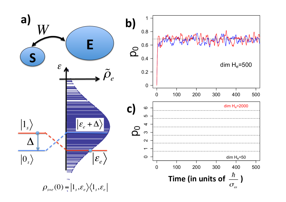
Figure 1: Emergence of the typical dynamics. Numerical simulations of the time evolution of the reduced density matrix of a system $S$ coupled to a quantum environment. a) Schematic representation of a system $S$ coupled to a large environment $E$, we consider here the particular case where $S$ is a two level system. The density of states of the environment $\tilde{\rho}_{e}$ is chosen to be gaussian distributed with standard deviation $\sigma_{e}=1$ and the gap of the two level system is $\Delta=1$. Written in the eigenbasis of $\hat{H}_{s}+\hat{H}_{e}$, the interaction $\hat{W}$ is an hermitian matrix such that $\{\operatorname{Re}(W_{i,j})\}_{i\geqslant j}$ and $\{\operatorname{Im}(W_{i,j})\}_{i>j}$ are independent centered gaussians with standard deviation $\sigma_{w}/\sqrt{2\dim\mathcal{H}}$ (providing $\operatorname{Tr}(W^{2})/\dim\mathcal{H}=\sigma_{w}^{2}$). b) From an initial pure state of the composite system $\varrho_{s+e}(0)=|1_{s}\rangle\langle 1_{s}|\otimes|\epsilon_{e}\rangle\langle\epsilon_{e}|$ (with $\epsilon_{e}\approx-1.27$ and $\dim\mathcal{H}_{e}=500$), we numerically integrate the Schrödinger equation and calculate the reduced density matrix of $S$: $\varrho_{s}(t)=\operatorname{Tr}_{e}(\varrho_{s+e}(t))$, for two different realizations of the random coupling $W$ (red and blue, with coupling strength $\sigma_{w}=0.2$). The probability for $S$ to be in its ground state $p_{0}=\langle 0_{s}|\varrho_{s}|0_{s}\rangle$ is plotted as a function of time. After a transient regime a stationary regime takes place characterized by a “speckle” pattern. This pattern is a signature of the microscopic structure of the interaction Hamiltonian. The theoretical prediction (black dashed line) is provided by Ithier and Benaych-Georges where an averaging procedure over $W$ (justified by measure concentration) allows to calculate analytically the typical stationary state of $S$: for the set of parameters considered here, one has $p_{0}\propto\tilde{\rho}_{e}(\epsilon_{e}+\Delta)$ and $p_{1}\propto\tilde{\rho}_{e}(\epsilon_{e})$. It should be noted that remarkably in this case, this prediction matches the one of the microcanonical ensemble. c) The dimension of the Hilbert space of the environment is varied from $50$ (black) to $2000$ (red) to show the concentration of measure phenomenon (predicted by Eq.(3)): the amplitude of the speckle pattern decreases and a typical asymptotic state emerges (curves are shifted vertically for clarity).

I Supplementary Material

I.1 Concentration of the reduced density matrix of the subsystem $S$

To use the Poincaré inequality in Eq.(1) and show that the reduced density matrix is concentrated, we calculate here:

• an adequate upper bound on the variance of the gradient of $\varrho_{s}(t)$ considered as a function of $W$,

• the Poincaré constants for the probability measures on spaces of interaction Hamiltonian we consider in this paper (WBRM and RRM).

As we will see, the upper bound on the gradient of $\varrho_{s}$ does not depend on the statistics chosen for $W$, meaning that our framework can be adapted to other classes of interaction Hamiltonians as soon as the Poincaré constant (or a lower bound) can be calculated for these classes.

I.1.1 1. Upper bound on the gradient square of $\varrho_{s}(t)$ considered as a function of the interaction.

In this section, our aim is to provide an upper bound on the norm of the gradient of $\rho_{s}$ considered as a function of $W$, which is uniform in the dimension. Recalling the definitions

$$|\psi\rangle\langle\psi|=U_{\tau}\rho(0)U_{\tau}^{\dagger}\qquad\text{and}\qquad U_{\tau}=e^{-i\tau(\hat{H}_{0}+\hat{W})},$$

with $\tau=t/\hbar$, we use the well known formula for the differential of the exponential map, in order to get the differential of $|\psi\rangle\langle\psi|$ with respect to the interaction $\hat{W}$:

$$\textbf{d}|\psi\rangle\langle\psi|(\delta W)=\int_{0}^{1}h\circ g_{\alpha}(\delta W)d\alpha$$

with

$$h(A)=-i\tau[A,|\psi\rangle\langle\psi|]\qquad\text{and}\qquad g_{\alpha}(B)=U_{\alpha\tau}\;B\;U_{\alpha\tau}^{\dagger}$$

where $[,]$ denotes the commutator and $\circ$ the composition of functions. We start by the upper bound

$$\small||\nabla_{W}\rho_{s}||^{2}=\left\|\int_{0}^{1}\operatorname{Tr}_{e}h\circ g_{\alpha}(\cdot)d\alpha\right\|^{2}\leqslant\int_{0}^{1}||\operatorname{Tr}_{e}h\circ g_{\alpha}(\cdot)||^{2}d\alpha$$

where the notation $||\cdot||$ is for the norm defined on the ensemble of linear applications from the space of interaction Hamiltonians to the space of density matrices on $\mathcal{H}_{s}$:

$$||f||^{2}=\sum_{i,j}||f(M_{i,j})||_{F}^{2}\quad\text{where}\quad||A||_{F}^{2}=\operatorname{Tr}(A.A^{\dagger}),$$

and

$$f:H_{\dim\mathcal{H}\times\dim\mathcal{H}}(\mathbb{C})\rightarrow H_{\dim\mathcal{H}_{s}\times\dim\mathcal{H}_{s}}(\mathbb{C}),$$

$H_{n,n}(\mathbb{C})$ is the ensemble of hermitian matrices of size $n\times n$ and $M_{i,j}$ is the matrix with zero everywhere except at the intersection of the $i^{th}$ line and $j^{th}$ column where it has a one. Then we have the equality:

$$\int_{0}^{1}||\operatorname{Tr}_{e}h\circ g_{\alpha}(\cdot)||^{2}d\alpha=||\operatorname{Tr}_{e}h(\cdot)||^{2}$$

since

$$\sum_{i,j}||f(M_{i,j})||_{F}^{2}=\sum_{i,j}||f(U.M_{i,j}.U^{\dagger})||_{F}^{2}$$

for any unitary matrix $U$. To move on and make the partial trace easy, we write $|\psi\rangle$ in the tensor basis $|\psi\rangle=\sum_{s,e}\gamma_{s,e}\;|\epsilon_{s}\rangle\otimes|\epsilon_{e}\rangle$ where $\{\gamma_{s,e}\}_{s,e}$ is a $\dim\mathcal{H}_{s}\times\dim\mathcal{H}_{e}$ matrix. Then we have for the matrix elements of $\operatorname{Tr}_{e}h(M_{a,b,c,d})$ where $M_{a,b,c,d}=|s_{a}\rangle\langle s_{b}|\otimes|e_{c}\rangle\langle e_{d}|$:

$$\langle\epsilon_{s}|\operatorname{Tr}_{e}[M_{a,b,c,d},|\psi\rangle\langle\psi|]|\epsilon_{s^{\prime}}\rangle=\gamma_{b,d}\;\gamma_{s^{\prime},c}^{*}\;\delta_{s,a}-\gamma_{s,d}\;\gamma_{a,c}^{*}\;\delta_{b,s^{\prime}}$$

Taking the square modulus and summing over $a,b,c,d$:

$$\small\sum_{a,b,c,d}|\langle\epsilon_{s}|\operatorname{Tr}_{e}([M_{a,b,c,d},|\psi\rangle\langle\psi|])|\epsilon_{s^{\prime}}\rangle|^{2}=\sum_{b\neq s^{\prime},c,d}|\gamma_{b,d}|^{2}|\gamma_{s^{\prime},c}|^{2}$$

$$+\sum_{a\neq s,c,d}|\gamma_{s,d}|^{2}|\gamma_{a,c}|^{2}+\sum_{c,d}|\gamma_{s^{\prime},d}\gamma_{s^{\prime},c}-\gamma_{s,d}\gamma_{s,c}|^{2}$$

$$=\left(\sum_{b,c,d}|\gamma_{b,d}|^{2}|\gamma_{s^{\prime},c}|^{2}+\sum_{a,c,d}|\gamma_{s,d}|^{2}|\gamma_{a,c}|^{2}\right)$$

$$-2\sum_{c,d}\operatorname{Re}\left(\gamma_{s^{\prime},d}\;\gamma_{s^{\prime},c}\;\gamma_{s,d}^{*}\;\gamma_{s,c}^{*}\right)$$

then summing over $s$ and $s^{\prime}$, we get the square of the norm we are looking for:

$$||\operatorname{Tr}_{e}h(\cdot)||^{2} = \tau^{2}\sum_{s,s^{\prime}}\sum_{a,b,c,d}\left|\langle\epsilon_{s}|\operatorname{Tr}_{e}([M_{a,b,c,d},|\psi\rangle\langle\psi|])|\epsilon_{s^{\prime}}\rangle\right|^{2}$$

$$= 2\tau^{2}\dim\mathcal{H}_{s}-2\tau^{2}\sum_{c,d,s,s^{\prime}}\operatorname{Re}\left(\gamma_{s^{\prime},d}\gamma_{s^{\prime},c}\gamma_{s,d}^{*}\gamma_{s,c}^{*}\right)$$

since the normalization condition provides $\operatorname{Tr}(\gamma.\gamma^{\dagger})=1$. The second term on the right hand side is:

$$\sum_{c,d,s,s^{\prime}}\left(\gamma_{s^{\prime},d}\gamma_{s^{\prime},c}\gamma_{s,d}^{*}\gamma_{s,c}^{*}\right)=\operatorname{Tr}((\gamma.\gamma^{\dagger})^{2})\geqslant 0$$

We finally get that

$$||\nabla_{W}\rho_{s}||^{2}\leqslant||\operatorname{Tr}_{e}h(\cdot)||^{2}\leqslant 2\tau^{2}\dim\mathcal{H}_{s}.$$

I.1.2 2. Poincaré constants for various probability measures on spaces of interaction Hamiltonians

The Poincaré constants are well known for the following probability measures:

• $N\times N$ Wigner Random Band Matrices.

  As a start, let us consider matrices with independent real centered Gaussian distributed entries. The Poincaré constant of the Gaussian probability measure $P$ of variance $\sigma^{2}$ on $\mathbb{R}$ is $1/\sigma^{2}$. It has the property of tensorizing: the Poincaré constant for the probability measure $P^{\otimes N}$ defined on $\mathbb{R}^{N}$ is the same: $1/\sigma^{2}$. The complex case is similar. As the entries of the matrices we consider have a typical variance $\sigma_{w}^{2}/N$ (to ensure $\operatorname{tr}(\hat{W}^{2})=\sigma_{w}^{2}$), the Poincaré constant will scale like $N/\sigma_{w}^{2}$. In the case of more general Wigner matrices: if the entries of a random matrix are independent and all satisfy a Poincaré inequality with the same constant, then the duly renormalized (i.e. divided by $\sqrt{N}$ ) matrix also satisfies, globally, a Poincaré inequality with constant in the scale $N$ (see Section 4.4.1 in G. Anderson (2009)). In addition, it is well known that if a random variable $X$ satisfies a P.I. with constant $m$, then the variable $\alpha X$ (with $\alpha$ fixed) will satisfy a P.I. with constant $m/\alpha^{2}$. From this property, we conclude that WBRM matrices, i.e. with entries having a variance profile of the type $W_{i,j}=a_{i,j}Y_{i,j}$ with $0\leq a_{i,j}\leq 1$ deterministic and $Y$ a Wigner matrix (with Poincaré constant $\geq m^{\prime}N$, $m^{\prime}$ fixed), will also satisfy a P.I. inequality with a constant $\geq m^{\prime}N$.

• Ensemble of $N\times N$ Randomly Rotated Matrices, i.e. of the type $\{U.D.U^{\dagger}\}$ where $D$ is a fixed diagonal matrix and $U$ is unitary or orthogonal Haar distributed random matrix.

  The Poincaré constant $C$ is actually related to the Ricci curvature of the ensemble considered as a manifold and the variance of the spectrum of $D$ (see appendix F. in G. Anderson (2009) and the results due to Gromov):

  $$C\geq\frac{N}{2\sigma_{D}^{2}}$$

  where $\sigma_{D}^{2}=\operatorname{Tr}(D^{2})/N$ is the variance of the spectrum of $D$ (which is assumed to be fixed).

To summarize: in all cases, because the variance of the spectrum $\hat{W}$ is set to a fixed value independent of the dimension $N$, the Poincaré constant of the probability measure of the matrix ensemble considered is lower bounded by $mN$ with $m$ fixed.

References

- Carnot (1824) S. Carnot, Réflexions sur la puissance motrice du feu et sur les machines propres à développer cette puissance (Bachelier, Paris, 1824).
- Boltzmann (1974) L. Boltzmann, Theoretical Physics and Philosophical Problems: Selected Writings, edited by B. McGuinness (Springer Netherlands, Dordrecht, 1974) Chap. The Second Law of Thermodynamics, pp. 13–32.
- Kubo et al. (1990) R. Kubo, H. Ichimura, T. Usui, and N. Hashitsume, Statistical Mechanics (North Holland Personal Library, 1990).
- Landau and Lifschitz (1980) L. D. Landau and E. M. Lifschitz, Course of Theoretical Physics (Pergamon, Oxford, 1980).
- J. Gemmer (2004) G. M. J. Gemmer, M. Michel, Quantum Thermodynamics: Emergence of Thermodynamic Behavior within composite quantum systems, Lecture in Physics, Vol. 1200 (Springer, 2004).
- Gemmer and Mahler (2003) J. Gemmer and G. Mahler, The European Physical Journal B - Condensed Matter 31, 249 (2003).
- (7) This phenomenon should not be confused with “entanglement concentration”, a different concept specific to quantum information theory.
- Talagrand (1996) M. Talagrand, Ann. Probab. 24, 1 (1996).
- Popescu et al. (2006) S. Popescu, A. J. Short, and A. Winter, Nature Physics 2, 754 (2006).
- Goldstein et al. (2006) S. Goldstein, J. L. Lebowitz, R. Tumulka, and N. Zanghi, Phys. Rev. Lett. 96, 050403 (2006).
- Reimann (2007) P. Reimann, Phys. Rev. Lett. 99, 160404 (2007).
- Linden et al. (2009) N. Linden, S. Popescu, A. J. Short, and A. Winter, Phys. Rev. E 79, 061103 (2009).
- vonNeumann (1929) J. vonNeumann, Z. Phys. , 30 (1929).
- Reimann (2016) P. Reimann, Nature Communications 7, 10821 (2016).
- Goldstein et al. (2010a) S. Goldstein, J. L. Lebowitz, C. Mastrodonato, R. Tumulka, and N. Zanghi, Proceedings of the Royal Society of London A: Mathematical, Physical and Engineering Sciences 466, 3203 (2010a).
- Goldstein et al. (2010b) S. Goldstein, J. L. Lebowitz, R. Tumulka, and N. Zanghi , The European Physical Journal H 35, 173 (2010b).
- (17) G. Ithier and F. Benaych-Georges, Typical equilibrium state of an embedded quantum system. In preparation.
- Dyson (1962) F. J. Dyson, Journal of Mathematical Physics 3, 140 (1962).
- Weiss (2012) U. Weiss, Quantum Dissipative Systems (World Scientific, 2012).
- Landau (1927) L. Landau, Z. Phys. 34 (1927).
- Flambaum et al. (1994) V. V. Flambaum, A. A. Gribakina, G. F. Gribakin, and M. G. Kozlov, Phys. Rev. A 50, 267 (1994).
- Fyodorov et al. (1996) Y. V. Fyodorov, O. A. Chubykalo, F. M. Izrailev, and G. Casati, Phys. Rev. Lett. 76, 1603 (1996).
- Weidenm ller and Mitchell (2009) H. A. Weidenm ller and G. E. Mitchell, Reviews of Modern Physics 81, 539 (2009).
- Mitchell et al. (2010) G. E. Mitchell, A. Richter, and H. A. Weidenm ller, Reviews of Modern Physics 82, 2845 (2010).
- Borgonovi et al. (2016) F. Borgonovi, F. Izrailev, L. Santos, and V. Zelevinsky, Physics Reports 626, 1 (2016).
- Porter (1965) C. E. Porter, Statistical Theories of Spectra: Fluctuations, edited by N. Y. Academy Press (1965).
- Brody et al. (1981) T. A. Brody, J. Flores, J. B. French, P. A. Mello, A. Pandey, and S. S. M. Wong, Reviews of Modern Physics 53, 385 (1981).
- Mehta (1991) M. L. Mehta, Random Matrices (Academic Press Inc, 1991).
- G. Anderson (2009) O. Z. G. Anderson, A. Guionnet, An Introduction to Random Matrices, Vol. 118 (Cambridge studies in advanced mathematics, 2009).
- Milman and Schechtman (1986) V. D. Milman and G. Schechtman, Asymptotic theory of finite-dimensional normed spaces, Lecture Notes in Mathematics, Vol. 1200 (Springer-Verlag, Berlin, 1986) pp. viii+156, with an appendix by M. Gromov.
- Flambaum et al. (1996) V. V. Flambaum, F. M. Izrailev, and G. Casati, Phys. Rev. E 54, 2136 (1996).
- Flambaum and Izrailev (2000) V. Flambaum and F. Izrailev, Phys. Rev. E 61 (2000).
- Kota (2014) V. K. B. Kota, Embedded Random Matrix Ensembles in Quantum Physics (Springer, 2014).
- Papenbrock and Weidenm ller (2007) T. Papenbrock and H. A. Weidenm ller, Reviews of Modern Physics 79, 997 (2007).
- Bloch et al. (2012) I. Bloch, J. Dalibard, and S. Nascimbène, Nature Physics 8, 267 (2012).
- Schreiber et al. (2015) M. Schreiber, S. S. Hodgman, P. Bordia, H. P. L schen, M. H. Fischer, R. Vosk, E. Altman, U. Schneider, and I. Bloch, Science 349, 842 (2015).
- Guhr et al. (1998) T. Guhr, A. M. Groeling, and H. A. Weidenmüller, Physics Reports 299, 189 (1998).