Fast approximate Bayesian inference for stable differential equation models

Abstract

Inference for mechanistic models is challenging because of nonlinear interactions between model parameters and a lack of identifiability. Here we focus on a specific class of mechanistic models, which we term stable differential equations. The dynamics in these models are approximately linear around a stable fixed point of the system. We exploit this property to develop fast approximate methods for posterior inference. We illustrate our approach using simulated data on a mechanistic neuroscience model with EEG data. More generally, stable differential equation models and the corresponding inference methods are useful for analysis of stationary time-series data. Compared to the existing state-of-the art, our methods are several orders of magnitude faster, and are particularly suited to analysis of long time-series ($>$10,000 time-points) and models of moderate dimension (10-50 state variables and 10-50 parameters.)

1 Introduction

Differential equations (DEs) are an integral part of modelling in many different scientific domains. The values of parameters in such models are key for providing theoretical predictions and interpreting experimental results. However, often external constraints on parameter ranges are weak and their values are known only with considerable uncertainty. From a methodological point of view, two important challenges for Bayesian inference in Stochastic DE (SDE) models are: (i) integrating out state variables to obtain the marginal likelihood for parameter values that drive the system dynamics; and (ii) designing effective proposals for efficiently exploring the parameter space. Pseudo-marginal algorithms, such as particle Markov chain Monte Carlo (MCMC) are focused primarily on the first of these challenges (Andrieu et al., 2010), Langevin and Hamiltonian Monte Carlo algorithms (Girolami and Calderhead, 2011; Hoffman and Gelman, 2014) on the second.

The difficulty of these challenges depends primarily on the following problem parameters: $n$, the number of time-points in the data-set; $d$, the dimension of the state-space; and $p$, the number of the unknown parameters. We are interested in problems that are difficult due to all of these, as this is typical for many modern applications of DE Models (DEMs). Attempts to reduce complexity are now often faced with systems where mathematical simplifications severely reduce the meaningfulness of the model to the domain scientist. Existing pseudo-marginal algorithms and Hamiltonian Monte Carlo methods do not scale well with these problem parameters. The state of the art methodology for accurate inference in such inference problems would be to combine these two classes of algorithms (Dahlin et al., 2015), but this approach still does not scale to the cases in which we are interested: namely where $d\approx 10$ to $50$, $p\approx 10$ to $50$, and $n>10^{4}$. This regime is common in many applications, including Computational Neuroscience and Systems Biology – see, e.g., Keener and Sneyd (1998); Murray (2002, 2003); Izhikevich (2007); Ermentrout and Terman (2010) and the references therein. For such applications, one of which may be found in Sec. 4, accurate inference using standard implementations of particle MCMC may take several months on a desktop computer.

Where “exact” inference is not computationally feasible, approximate methods may still be. However, because parameters are often not identifiable in DEMs (Golowasch et al., 2002), methods that solely find point estimates of parameters or Laplace approximations to the posterior are not appropriate (see the discussion of sloppiness in Girolami and Calderhead (2011)). Approximating the posterior marginals (as in variational, expectation propagation or the integrated nested Laplace methods) is also not appropriate, since the dependency structure in the posterior often is of more interest than the posterior marginals themselves. In this paper we present an approximate but scalable alternative. In order for it to be accurate, we need to place restrictions on the allowed dynamical behaviour. Specifically, we consider here only system dynamics in the vicinity of stable equilibrium points. There is a good range of applications where such models are used. Our showcase application is the analysis of an electroencephalogram (EEG) time-series using a mechanistic model. We improve on existing methodology for this application, which can be found in Moran et al. (2009); Pinotsis et al. (2012a); Abeysuriya and Robinson (2016).

The innovations in this paper concern both the estimation of the marginal likelihood of the parameters, and the exploration of the parameter space. The spectral density of systems linearized around a stable equilibrium point can be calculated analytically, rather than by direct numerical solution. Making use of this fact and the Whittle likelihood, we can reduce the computational effort required to calculate the marginal likelihood by orders of magnitude. Furthermore, we introduce heuristics that quantify the accuracy of these approximations. Exploring the parameter space can be dramatically simplified by a reparameterization that uses equilibrium values as model parameters, which often results in a reduction of computational effort by an additional order of magnitude. Finally, we find derivatives of our Whittle likelihood analytically in order to use gradient-based Monte Carlo methods for efficient exploration.

In the following Sec. 1.1, we describe more precisely the class of models to which the methods in this paper are directly applicable. Section 2 introduces the main methodological innovations. Section 3 then illustrates the properties of our new approach with the well known FitzHugh-Nagumo equations (FitzHugh, 1961; Nagumo et al., 1962; Izhikevich, 2007). Section 4 then applies our method to a more challenging parameter inference problem from computational neuroscience.

1.1 Stability and stochasticity in nonlinear dynamical systems

A general form for many continuous-time nonlinear dynamical systems is

$$\frac{d}{dt}\mathbf{x}(t)=\mathbf{F}[\mathbf{x}(t);\theta]+\mathbf{p}(t;\theta),$$ (1)

where $\mathbf{x}$ is a vector of states with length $d$, $\theta$ is a vector of parameters, and $\mathbf{F}$ is a vector-valued nonlinear function, also with $d$ components. This form separates the time-invariant “system” given by $\mathbf{F}$ and $\theta$ from an explicitly time-dependent “input” $\mathbf{p}$. Aspects of many natural and engineered systems are approximated well by this form, due to large differences in the time-scales of other processes. For example, brain connectivity changes considerably over a human lifetime, but typically can be considered as a static structure for the description of neural processes lasting milliseconds to seconds.

If $\mathbf{p}(t;\theta)$ is a deterministic function, then Eq. (1) represents a system of coupled Ordinary DEs (ODEs). This is particularly appropriate if we model a stimulus (a distinct event, or series of events) through the input $\mathbf{p}(t;\theta)$. We then assume that $\mathbf{p}(t;\theta)$ is zero as default, but becomes non-zero in a characteristic way at times when the system receives a stimulus. If $\mathbf{p}(t;\theta)$ is the time derivative of Brownian motion, then Eq. (1) represents a multivariate diffusion process with drift term $\mathbf{F}[\mathbf{x};\theta]dt$. The conventional notation for diffusion processes can be obtained by multiplying through by $dt$, and setting $\mathbf{p}(t;\theta)dt=\Sigma(\theta)d\mathbf{B}_{t}$, with $\Sigma(\theta)$ a diagonal matrix, and $\mathbf{B}_{t}$ standard uncorrelated multivariate Brownian motion. We assume that $\mathbf{p}(t;\theta)$ has mean zero. Such an SDE is particularly appropriate for “resting state” conditions, where the system is not primarily driven by separable and characteristic events (at least to our knowledge), but noisy internal and/or external fluctuations dominate.

A further distinction that is key for this paper is between what we refer to as stable and unstable systems. To understand these labels, we first have to discuss the so-called equilibrium or fixed points of a system. A point $\mathbf{x}^{*}$ is an equilibrium point of the system dynamics if its state remains constant in this point: $\left.d\mathbf{x}/dt\right|_{\mathbf{x}=\mathbf{x}^{*}}=0$. To be more specific, we consider here equilibrium points for “least input” scenarios: in the absence of all stimuli (deterministic case) or for exactly average input (stochastic case), respectively. In both cases, we would set $\mathbf{p}(t;\theta)\equiv 0$ in Eq. (1) due to our definition of the input term above. The equilibria are then solutions of $\mathbf{F}[\mathbf{x}^{*};\theta]=0$. The stability of an equilibrium point is evaluated by examining the eigenvalues of $\mathcal{J}$, the Jacobian matrix of $\mathbf{F}$ evaluated for $(\mathbf{x}^{*};\theta)$. The condition for stability of an equilibrium point is

$$\max_{n=1,\ldots,d}(\mathrm{Re}[\lambda_{n}])<0,$$ (2)

where $\lambda_{1},\ldots,\lambda_{d}$ are the eigenvalues of $\mathcal{J}(\mathbf{x}^{*};\theta)$. The Jacobian is calculated by taking the partial derivatives of $\mathbf{F}$ with respect to the state variables

$$[\mathcal{J}]_{ij}(\mathbf{x}^{*},\theta)=\left.\frac{\partial[\mathbf{F}]_{i}(\mathbf{x};\theta)}{\partial[\mathbf{x}]_{j}}\right|_{\mathbf{x}=\mathbf{x}^{*}}.$$ (3)

In the following we will be concerned with methods for systems evaluated near such a stable equilibrium. We refer to a system as “stable” in the following if it possesses at least one stable equilibrium point. There may be some regions of the parameter space where the system has no stable equilibrium points. However, provided that one can find a region in the available parameter space where it does, then we still call this a “stable” case – with the implicit understanding that our parameter inference is valid only in a region of parameter space with at least one stable equilibrium. While our methods are applicable to all such stable systems, the accuracy of posterior inference depends both on the model and on the magnitude of the input to the system. We consider this in more detail in Sec. 3.2. Furthermore, we present computationally efficient ways of determining whether the approximation is accurate for a given problem.

The reparameterization method presented in this paper is applicable to both stable ODEs and stable SDEs. A necessary, but not sufficient, condition for the method to be effective is that the system returns to its stable equilibrium following transient input. This is guaranteed if there is only one stable equilibrium and the system returns to that equilibrium when initialized from any other point in the state space. When there is more than one attractor state, then the system will return to the same equilibrium point if the input / stimulus is sufficiently small. Spectral analysis using the Whittle likelihood is applicable to stable SDEs. The methodology we present for rapidly calculating the spectral density requires the model to be linearized. It is therefore only applicable when the input is sufficiently small for the the linearized model to be a good approximation to the nonlinear model. A classic example is the description of a pendulum as harmonic oscillator, which is valid as long the angle of its swings are small enough for $\sin\phi\approx\phi$.

The dynamics of mesoscopic brain oscillations in the resting state, as measured for example with the electroencephalogram (EEG), are a prominent case in point (van Rotterdam et al., 1982; Liley et al., 2002; Breakspear and Terry, 2002). Generally speaking, many nonlinear systems have operating regimes of interest where the system dynamics are thought to be (or are designed to be) quasi-linear, as guaranteed by the local stable manifold theorem (Kelley, 1967). Note that linearizing around an equilibrium point is different from repeatedly linearizing the model around a sequence of distinct points in the state-space. In general linearizing around an equilibrium point will be more approximate because the linearization is only accurate when the system is close to its equilibrium state, cf. Section IV of Bojak and Liley (2005). The effect of this approximation on posterior inference is examined empirically in Sec. 3.2.

2 Methodology

2.1 Model reparameterization: equilibrium values as parameters

A dynamical system is specified by supplying a set of parameters $\mathbf{\theta}$. Hence, generally its equilibria $\mathbf{x}^{*}$ will be a function of these $\mathbf{\theta}$. For the form in Eq. (1) discussed above, this follows from solving $\mathbf{F}[\mathbf{x}^{*};\theta]=0$. For stable ODEs, $\mathbf{x}^{*}$ does not explicitly enter the likelihood calculations. Nevertheless, the likelihood is implicitly a function of $\mathbf{x}^{*}$, and it can be more sensitive to values of $\mathbf{x}^{*}$ than to values of $\mathbf{\theta}$. For stable SDEs, the likelihood calculations we use depend on linearizing the system around $\mathbf{x}^{*}$. In this case the likelihood is explicitly a function of $\mathbf{x}^{*}$.

In this paper we use an MCMC algorithm to explore the posterior on $\theta$, and find that the posterior may be explored more efficiently by reparameterizing the model such that $\mathbf{x}^{*}$ is treated directly as a parameter of the model. Thus rather than treating $\mathbf{x}^{*}$ as a function of $\theta$ (as in the original parameterization), some elements of $\mathbf{\theta}$ can be calculated as a function of $\mathbf{x}^{*}$. If $\mathbf{\theta}$ is of dimension $d_{\theta}$ and $\mathbf{x}^{*}$ of dimension $d_{x}$, then the combined parameter space $(\mathbf{\theta},\mathbf{x}^{*})$ has dimension $d_{\theta}+d_{x}$ but only $d_{\theta}$ degrees of freedom. One could choose any combination of $d_{\theta}$ parameters to parameterize the model. Then the remaining $d_{x}$ parameters would be a function of the chosen $d_{\theta}$ parameters. We therefore introduce the subscripts $s$ and $d$ to distinguish between these parameter subsets: the MCMC is applied to the reparameterized space $\theta_{s}$, with $\theta_{d}$ being a deterministic function of $\theta_{s}$.

As an example, suppose that the equations for the equilibrium points were of the simple form

$$\mathbf{F}[\mathbf{x}^{*},\mathbf{\theta}_{s}]+\mathbf{\theta}_{d}=0,$$ (4)

where $\mathbf{F}$ is a nonlinear function with $d_{x}$ components, $\mathbf{\theta}_{d}$ is a vector of parameters also with $d_{x}$ elements, and $\mathbf{\theta}=(\mathbf{\theta}_{s},\mathbf{\theta}_{d})$. Then we can simply reparameterize the model in terms of $(\mathbf{\theta}_{s},\mathbf{x}^{*})$, and calculate $\mathbf{\theta}_{d}=-\mathbf{F}[\mathbf{x}^{*}_{s},\mathbf{\theta}_{s}]$. Let us compare the form in Eq. (4) with the one that arises for our systems of interest from Eq. (1). Note that above we had defined $\mathbf{p}(t;\theta)\equiv 0$ as default for the input. What if instead either stimuli or resting state fluctuations occurred on top of some constant background input $\overline{\mathbf{p}}+\mathbf{p}(t;\theta)$? We can bring this into our standard form by absorbing the constant background input $\tilde{\mathbf{F}}[\mathbf{x},\theta]\equiv\mathbf{F}[\mathbf{x},\theta]+\overline{\mathbf{p}}$, and using $\tilde{\mathbf{F}}$ instead in Eq. (1). Then solving for equilibria of $\tilde{\mathbf{F}}[\mathbf{x};\theta]=0$ naturally has the form of Eq. (4), with the background input $\overline{\mathbf{p}}$ serving as the $\mathbf{\theta}_{d}$. Our method can also be applied in cases when the dimensions of $\mathbf{F}$ and $\mathbf{\theta}_{d}$ do not coincide, i.e., if the background input is added only to some equations. It then still may be possible to obtain closed form expressions for $\theta_{d}$ in terms of $\mathbf{x}^{*}$ and $\theta_{s}$, as for the example given in Sec. 4. Mathematical details of this more involved case can be found in the supplementary Sec. S2.1.

How can such reparameterizations be advantageous? Likelihood distributions for DEMs are typically complicated, with strong dependencies – linear and/or nonlinear – between model parameters. If equilibrium values have weaker nonlinear dependencies with model parameters than model parameters do with each other then the posterior will be simplified when the model is reparameterized,. Consequently, fewer MCMC iterations will be required. Furthermore, for a reparameterization in closed form the computational cost per MCMC iteration is reduced further, since it is then not necessary to solve a nonlinear system of equations for the equilibrium.

Some issues that arise when designing a sampler on the reparameterized space are (i) correctly evaluating prior densities and proposal densities, (ii) ensuring that the proposal does not frequently propose parameter sets outside the support of the prior, and (iii) in the case of multiple stable equilibria, choosing which one to use. These issues can all be dealt with in a principled way, cf. Sec. S2.1, and do not limit the scope of applicability of our methods in practice.

2.2 The spectral density of stable SDEs

If $x^{T}(t)$ is a component of the multivariate stochastic process $\mathbf{x}(t)$ measured over time interval $T$, then the (power) spectral density of $x(t)$ can be estimated with

$$S_{xx}(\nu)=\frac{1}{T}\left|X^{T}(\nu)\right|^{2},$$ (5)

where $X^{T}(\nu)$ denotes the Fourier transform of $x^{T}(t)$ with ordinary frequency $\nu$. In applications one typically measures $n$ samples of $x(t)$ during $T$ at regular intervals $\Delta t=T/n$. The (power) spectral density is then estimated as

$$\frac{1}{\Delta t}S_{xx}\left(\nu=\nu_{k}\equiv k/T\right)\quad\longrightarrow\quad S_{k}=|X_{k}|^{2},$$ (6)

with $k=0,...,n-1$ and the Discrete Fourier Transform (DFT) $X_{k}$ of these samples.

Stable SDEs can be approximated by linearizing around a fixed point. For the linearized system, one can relate the Fourier transform of the noise (input) $\mathbf{P}$ to that of the state (output) $\mathbf{X}$

$$\mathbf{X}(\nu)=\mathcal{T}(\nu)\cdot\mathbf{P}(\nu),$$ (7)

where the matrix $\mathcal{T}$ that maps $\mathbf{P}$ to $\mathbf{X}$ is called the transfer function. An analytic expression for $\mathcal{T}$ can be obtained using the eigen-decomposition of $\mathcal{A}$ (Bojak and Liley, 2005). We can use these analytic results to rapidly compute (spectral) model predictions

$$\mathbf{f}(\nu_{k})\equiv\frac{1}{\Delta t}\left|\mathcal{T}(\nu_{k})\cdot\mathbf{P}(\nu_{k})\right|^{2},$$ (8)

which can be directly compared with the measured $S_{k}$. Analytic derivatives of the modeled spectral density can also be calculated. Section S2.2 in the supplement contains a detailed discussion of these estimation methods. The computational complexity of the spectral density calculation is $\mathcal{O}(d^{3})$. The computational savings that can result from working in the frequency-domain as opposed to the time-domain are discussed in Sec. S2.3.3.

Table 1: MCMC algorithms used to generate results in Secs. 3 and 4

Algorithm Name	Applicability	Likelihood
MwG	nonlinear ODEs	Eq. (S26)
Particle Marginal MwG	nonlinear SDEs	MC of Eq. (11)
Kalman Marginal MwG	linearized SDEs	Eq. (11)
Whittle smMALA	linearized SDEs	Eq. (12)

2.3 Whittle likelihood for SDEs

In this section we describe our novel methodology for inference in SDEs with a stable equilibrium point. We use an MCMC framework, where calculating the likelihood of the parameters requires integrating over the state space. The resulting marginal likelihood estimate enters into the acceptance ratio of MCMC algorithms for parameter estimation. Details of the MCMC algorithms (Metropolis-within-Gibbs, MwG, and simplified manifold MALA, smMALA) used in this paper can be found in the supplementary Sec. S2.4. In Tab. 1 we list the variants of MwG and smMALA used to generate our results.

The novelty in our approach lies in the way that the contributions in Secs. 2.1 and 2.2 are used within existing MCMC methodology. We will apply the Whittle likelihood (Whittle, 1962) to stable DEMs of the form

$$\mathrm{d}\mathbf{x}(t) =\mathrm{F}\left[\mathbf{x}(t);\theta\right]\mathrm{d}t+\Sigma(\theta)\mathrm{d}\mathbf{B}_{t}$$ (9)

$$\mathbf{y}_{i} =\mathrm{L}(\mathbf{x}_{i};\theta)+\mathbf{n}_{i}(\theta)$$ (10)

where $\mathbf{y}_{i}$ is a vector of observations at the discrete time index $i$ of the system state $\mathbf{x}_{i}\equiv\mathbf{x}(t=t_{i})$, $\mathrm{L}$ is a linear function, and $\mathbf{n}_{i}$ is a discrete-time process for which it is possible to compute the spectral density, the simplest example of which is white noise. The parameter set, $\theta$, now includes parameters that influence the observation process, $\mathbf{n}_{i}(\theta)$, as well as $\mathrm{F}[\mathbf{x}(t);\theta]$ and $\Sigma(\theta)$.

The Whittle likelihood approximates the marginal likelihood,

$$p_{\theta}(y_{1:n})=\int p_{\theta}(y_{1:n}|x_{1:n})p_{\theta}(x_{1:n})\,dx_{1:n}.$$ (11)

In Sec. S2.3.3 of the Supplement we summarize how this likelihood can expressed purely in terms of the theoretical frequency representation $\tilde{f}(\nu_{k};\theta)$, depending on model parameters $\theta$, and the empirical one $\tilde{S}_{k}$ derived from data, without referring at all to the time domain:

$$p_{\theta}(y_{0},\ldots,y_{n-1})=p_{\theta}\left(\tilde{S}_{0},\ldots,\tilde{S}_{n-1}\right)\approx\prod_{k=1}^{n/2-1}\frac{1}{\tilde{f}(\nu_{k};\theta)}\exp\left[-\frac{\tilde{S}_{k}}{\tilde{f}(\nu_{k};\theta)}\right].$$ (12)

Both frequency representations take into account Eq. (10), e.g., if only white noise is added then $\tilde{f}(\nu_{k};\theta)=f(\nu_{k};\theta)+\mathrm{const.}$

Linearization of the model around a stable equilibrium point (described in Sec. S2.2) yields a stationary approximate model for which the spectral density exists, and which we may differentiate analytically. Our main reason for using the Whittle likelihood is that we may exploit a computational saving in the case of evaluating the spectral density of a partially observed SDE, cf. supplementary Sec. S2.2. In the cases considered in this paper in which only a single variable is observed, evaluating the spectral density at $n$ points (as we do in the Whittle likelihood) has complexity $\mathcal{O}(nd)$, which compares favourably to the $\mathcal{O}(nd^{3})$ complexity of the Kalman filter. We further note that the use of the Whittle likelihood may be intuitive to practitioners, who are often familiar with a frequency domain representations of their data. For example, quantitative studies of the electroencephalogram (EEG) often make use of the (power) spectral density.

The approximation made by the Whittle likelihood is two-fold. First, the model is linearized at a stable fixed point of the system. Second, the likelihood of the linearized model is approximated in the frequency domain by Eq. (12). See Sec. S2.3.3 in the Supplementary for more details. Both of these approximation errors can be quantified, as we show in Sec. 3.2 and supplementary Sec. S3.2. The linear approximation is well suited to SDEs operating close to a stable equilibrium as the dynamics are approximately linear in this case. When this condition is not satisfied, a more appropriate choice of likelihood estimate is the particle filter (Gordon et al., 1993), an importance-sampling Monte Carlo method that yields an unbiased approximation of the marginal likelihood up to discretization error. The particle filter approach is often accurate, but is usually computationally expensive. See Sec. S2.3.1 in the Supplementary for more details.

For linear models the marginal likelihood can be evaluated exactly using the Kalman filter. By numerical experimentation, cf. Sec. S3.2 in the Supplement, we have found that the Kalman filter and Whittle likelihood posteriors are similar when

$$\frac{\phi}{n} <0.01\max_{k}\left[f(\nu_{k})\right],$$ (13)

$$\phi \equiv\sum_{h=-\infty}^{\infty}|h|\left|\gamma_{xx}(h\cdot\Delta t)\right|,$$ (14)

where $\gamma_{xx}(\tau)$ is the autocovariance function. This is illustrated in Fig. S4 in the Supplement. Since it is quicker to compute this than to do a full comparison between posterior distributions, we recommend using Eq. (13) as a heuristic rule to decide whether the Whittle likelihood is a sufficiently accurate approximation to the true likelihood. For the example in Sec. 4, estimating the posterior distribution using the Kalman filter is intractable and we rely on the heuristic in Eq. (13) to give an indication of whether the Whittle likelihood is accurate.

3 Analysis using the FitzHugh-Nagumo equations

The FitzHugh-Nagumo (FHN) model (FitzHugh, 1961; Nagumo et al., 1962; Izhikevich, 2007) is a highly simplified description of neural activity and exhibits nonlinear oscillations. These equations have been used before to test methodology for general nonlinear problems (Girolami and Calderhead, 2011; Jensen et al., 2012). In this section, we use the FHN system to illustrate the properties of our approach, comparing it with existing ones. We begin in Sec. 3.1 (details in the supplementary Sec. S3.1) by using a deterministic FHN variant in order to illustrate the improvement in efficiency of Metropolis-within-Gibbs when run on a reparameterized model. Next in Sec. 3.2, we study a stochastic version of the FHN model in order to compare the use of the three time domain likelihoods described in Secs. S2.3.3 and S2.3, namely the particle filter, the extended Kalman filter, and the Kalman filter with a time-homogeneous linearization of FHN about a stable equilibrium point.

There are parameter sets for which the FHN model has a stable equilibrium point, and where, given a sufficiently large perturbation away from the stable equilibrium, the model produces a nonlinear transient oscillation. There are also parameter sets where a sufficiently large perturbation from stable equilibrium can cause the the system to move towards a limit-cycle attractor. However, we do not consider that case here. The FHN equations that we will use here are

$$\frac{d}{dt}V(t) =V(t)[a-V(t)][V(t)-1]-w(t)+I_{0}+I(t)$$ (15)

$$\frac{d}{dt}w(t) =bV(t)-cw(t)+d+P(t).$$ (16)

We assume the following observation model,

$$y_{i}=V(t_{i}=i\cdot\Delta t)+n_{i}$$ (17)

where $\Delta t$ is some constant time-step and the $n_{i}$ are i.i.d. normal random variables, for $i=0,\ldots,n-1$.

The state variables $V$ and $w$ are referred to as the membrane potential and the recovery variable, respectively, when the model is used in the neuroscience domain. Compared to the standard FHN form (FitzHugh, 1961; Nagumo et al., 1962; Izhikevich, 2007), we have added here terms $d$ and $P(t)$ to the recovery variable, to allow additional analysis below. However, this is not intended as a new model proposal in the domain science, and obviously the standard form will be recovered if these terms are set to zero. Furthermore, as discussed in Secs. 1.1 and 2.1, we intend $P(t)$ to be zero by default in the ODE and mean-zero in the SDE case, with $d$ parameterizing any constant perturbation. Similarly, we consider $I(t)$ here as zero by default / mean-zero, and hence in comparison to the standard notation have explicitly separated out a possible constant input as $I_{0}$.

Here and in the following we always consider equilibria for default inputs $P(t)=I(t)=0$. The steady-state equations, also known as nullclines, are then obtained by setting the derivatives $dV/dt$ and $dw/dt$ to zero. If constant inputs $d$ and $I_{0}$ are absent as well, then it is easy to see from Eqs. (15) and (16) that there is an equilibrium at $V^{*}=w^{*}=0$. As shown, equilibrium values of state variables will be indicated by a star superscript. This particular equilibrium will be stable if $a+c>0$ and and $ac+b>0$, as follows from computing the eigenvalues of the Jacobian:

$$\mathcal{J}=\begin{pmatrix}-a&-1\\ b&-c\\ \end{pmatrix}.$$ (18)

There are multiple ways to reparameterize the model, and the most appropriate choice depends on the inference problem. If both $V$ and $w$ were observed, and the aim was to infer $(a,b,c,d,I_{0})$, we would update $V^{*}$ and $w^{*}$ using the MCMC proposal and then, given the values of $V^{*}$ and $w^{*}$, solve for the inputs $d$ and $I_{0}$:

$$I_{0} =-V^{*}(a-V^{*})(V^{*}-1)+w^{*}$$ (19)

$$d =-bV^{*}+cw^{*}$$ (20)

In the MCMC algorithm for the reparameterized model, the updates for $(a,b,c,V^{*},w^{*})$ would be stochastic with a Metropolis-Hastings kernel. The updates for $(I_{0},d)$ would be deterministic using Eqs. (19) and (20). Alternatively, if only $V$ was observed and $d$ was known we would update only $V^{*}$ using the MCMC proposal since the likelihood is no longer sensitive to the value of $w^{*}$. In this case the value of $w^{*}$ is determined through the other parameters, and we solve for $I_{0}$:

$$w^{*} =\frac{1}{c}(bV^{*}+d)$$ (21)

$$I_{0} =-V^{*}(a-V^{*})(V^{*}-1)+w^{*}$$ (22)

When the model is not reparameterized, the equilibria can be obtained by solving a cubic equation for $V$, and then substituting these values into a linear equation for $w$. The coefficients of the cubic $V\/$-nullcline depend on all of the parameters, hence the steady-states are then nonlinear functions of the model parameters. For a given set of parameters, the system can have more than one stable equilibrium. We define a unique mapping from parameters to equilibrium by selecting the steady-state $V$-component that is closest to the mean of the $V\/$-observations.

There are some scenarios where the model parameters of the FHN model are not identifiable from the data. In results for the FHN model, we consider a scenario where the model parameters are identifiable as this eases visualisation and interpretation. In the more challenging scenario where the parameters are not identifiable from the data we recommend using the prior distribution to stabilize the variance of the posterior distribution. Our analysis of a Neural Population Model in Sec. 4 is an example of this.

3.1 Results for deterministic FitzHugh-Nagumo equations

From Sec. 3.2 onwards, we focus on stable SDEs, where both the methodology on model reparameterization and likelihood approximation can be applied. Here we briefly summarize the results of applying the reparameterization methodology to the deterministic FitzHugh-Nagumo equations. For certain parameter sets this model has a stable fixed point, and is therefore a stable ODE. As measured by differences in the ESS, the Metropolis-within-Gibbs algorithm is faster by a factor of around 14 when the model is reparameterized, as shown in Tab. 2. Further details on the model parameters and MCMC samples are given in Sec. S3.1 of the Supplement.

	Original parameterization		Steady-state reparameterization
Parameter	Proposal s.d.	ESS	Proposal s.d.	ESS
$a$	5	13	3.5	175
$b$	250	22	250	144
$c$	1	10	3	174
$I_{0}$	2.5	9	n/a	249
	Average ESS	13.5	Average ESS	185.5

Table 2: Results for Metropolis-within-Gibbs MCMC algorithm with and without reparameterization. Total number of MCMC iterations was 100,000. ESS was calculated on the second half of the samples (i.e., the last 50,000 samples) to remove the effects of burn-in. Proposal standard deviation (s.d.) for $V^{*}$ in the reparameterized algorithm was 0.015.

3.2 Evaluating posterior accuracy under linearized model

As discussed in Sec. S2.3.3, the Whittle likelihood approximates the marginal likelihood, $p_{\theta}(y_{1:n})$. The purpose of this section is to examine the accuracy of this approximation in more detail. We first look at errors arising from linearizing the model, using the stochastic FitzHugh-Nagumo equations as an example. We are interested in cases when the dynamics of the nonlinear model are approximately linear around some stable equilibrium. As discussed in supplementary Sec. S2.2, the accuracy in the approximation depends on the magnitude of the input to the system, as this determines the amplitude of the system dynamics. For a given set of system parameters, the linearization can be made arbitrarily accurate by choosing a small enough magnitude for the input. However, this is not a strong enough result to guarantee accurate posterior inference. Suppose that the linearization is accurate for the true system parameters and the true input parameters. There may be regions of the parameter space where the likelihood is high under the linearized model but the linearization is inaccurate. For example, if a dynamical system has two stable fixed points and the magnitude of the noise that feeds into the system is sufficiently large, the system can transition between approximately linear dynamics around one fixed point to approximately linear dynamics around the other fixed point. In the linearized model, the system always stays relatively close to the stable equilibrium point that the system was linearized around. It is not uncommon in dynamical systems models for the behaviour of the system to be different in different regions of the parameter space. Hence, for one parameter set the dynamics of the nonlinear model are approximately linear around a single fixed point, but for a different parameter set the system switches between two different fixed points.

empty

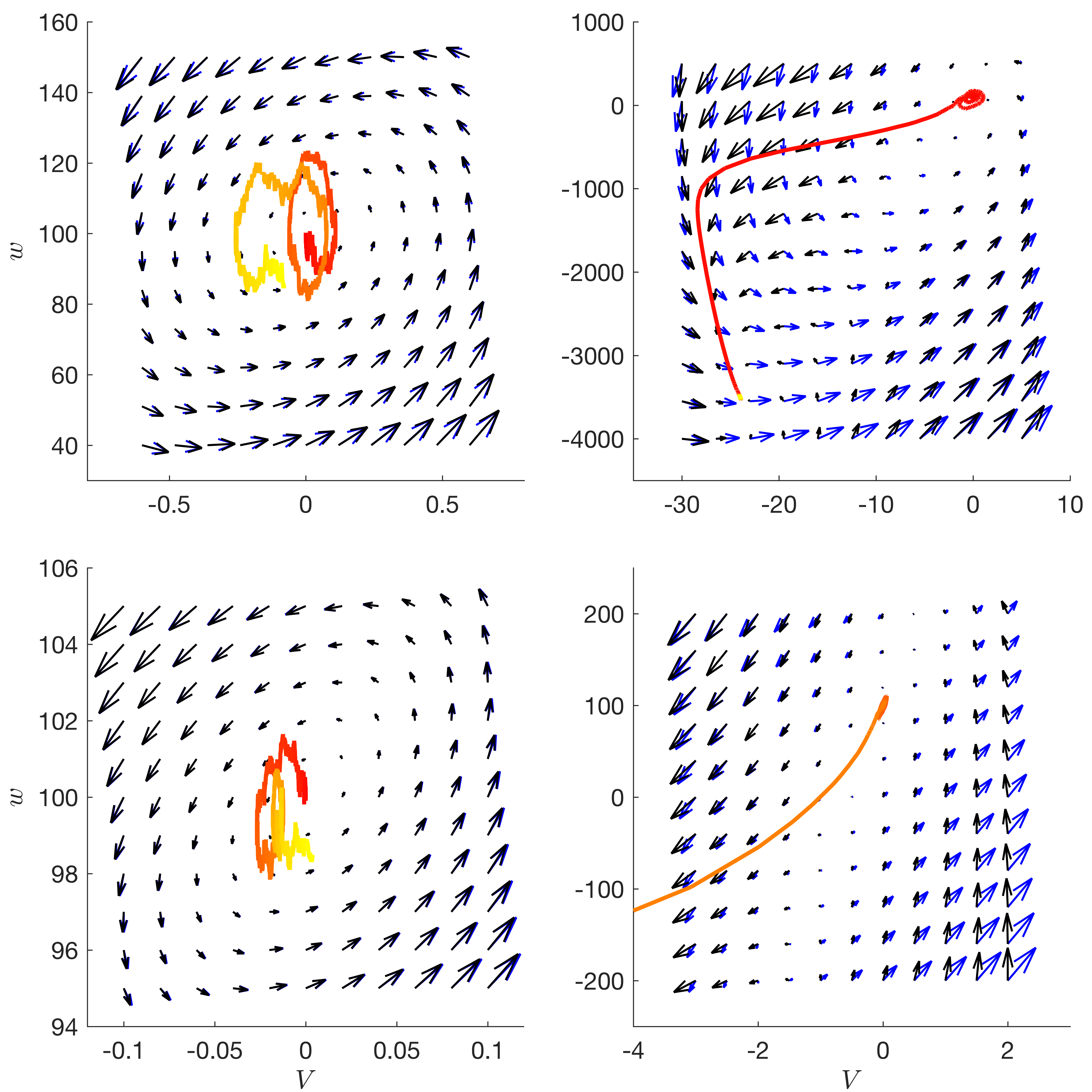
Figure 1: Vector fields for the FitzHugh-Nagumo model (black arrows) and its linearization around a stable equilibrium (blue arrows), as well as sample path of nonlinear model (coloured line). Arrows represent the drift term, i.e., the deterministic time-derivative. Left column: Nonlinear model is well approximated by linearization. Right column: Linearized model is not a good approximation in spite of similar likelihood compared to the cases on the left, cf. see Figs. 2 and 3. $I(t)=0$ and $P(t)$ was white noise with variance $\sigma_{in}^{2}$. Top left parameter values for $(a,b,c,d,I,\sigma_{in})$: $(-5,6000,40,4000,100,100)$. Top right: $(-30,6000,40,4000,100,100)$. Bottom left: $(-30,6000,40,4000,100,10)$. Bottom right: $(-150,3000,170,17000,100,10)$.

This is illustrated using a stochastic FitzHugh-Nagumo model in Fig. 1. It shows in the top left panel a case with only one equilibrium point where the linearization works well. In the top right panel we see that under the change of just one parameter linearization and nonlinear model cease to agree well: the nonlinear model escapes to a different equilibrium point, which is not predicted by the linearization. In the bottom left panel we see that reducing the input noise by a factor of ten stabilizes the agreement again. However, the bottom right panel demonstrates that one can change more parameters to remove agreement again even at these low input noise levels. It should be noted however that if we had linearized around the second equilibrium point in Fig. 1 top right – the one to which the nonlinear model escapes – then we would have found agreement even at the high noise levels. Clearly the appropriateness of the linearization in a situation with multiple equilibria has to be confirmed on a case by case basis.

In order to quantify the error caused by the linearization we ran both MCMC using a Kalman filter to estimate the likelihood (i.e. marginal MCMC), and particle MCMC, on data simulated from the FitzHugh-Nagumo model. We found the posterior distribution was noticeably broader in the marginal MCMC samples, i.e., in the algorithm where the model was linearized (results not shown). This discrepancy necessitated further empirical investigation, however this was constrained by the fact that the computational cost of running particle MCMC on the FitzHugh Nagumo model was very high (requiring more than one month of computing time on a cluster of 20 cores). This can be reduced, for example by using a low-level language, e.g., C, a more sophisticated variant of particle MCMC, e.g., a proposal that makes use of the next data-point, or by implementation on a computing environment where greater parallelism is possible, e.g., GPUs. All of these options are (currently) expensive in terms of user-time, thus were not pursued here.

As an alternative to comparing with particle MCMC, the following checks are useful for partially quantifying the error that comes from linearizing the model: (i). Compare marginal likelihood estimates from the basic Kalman filter (i.e. linearizing about the stable point), Extended Kalman Filter (EKF), and particle filter on a 1-D grid for each individual parameter. (ii). Compare the posterior distribution obtained from running marginal MCMC with the Kalman filter to marginal MCMC with the EKF. (iii). Simulate from the linearized model and the nonlinear model at parameter sets sampled by marginal MCMC to check for nonlinear dynamics. These require much less computing time than running particle MCMC, and are also relatively easy to implement. We performed these checks for several scenarios with the aim of investigating the effect of our approximations.

In summary, when performing linearization around a fixed point we have observed the following useful properties: (i). There is only a small difference using the Kalman filter (in which the linearization is about a stable point) and the EKF when the input noise is small - Figure 2. (ii). As more data is collected, the posterior variance decreases at approximately the same rate with the approximate and exact methods - Figure 2. (iii). Our approximate posterior distribution tends to accurately capture the qualitative dependency structure between parameters - Figure 3. (iv). Where the likelihood differs between the Kalman filter and the EKF, we find that our approach tends to over-estimate uncertainty - Figure 3. This makes our approximation suitable for embedding within an exact approach to speed it up (e.g., using importance sampling or delayed acceptance (Golightly et al., 2014)).

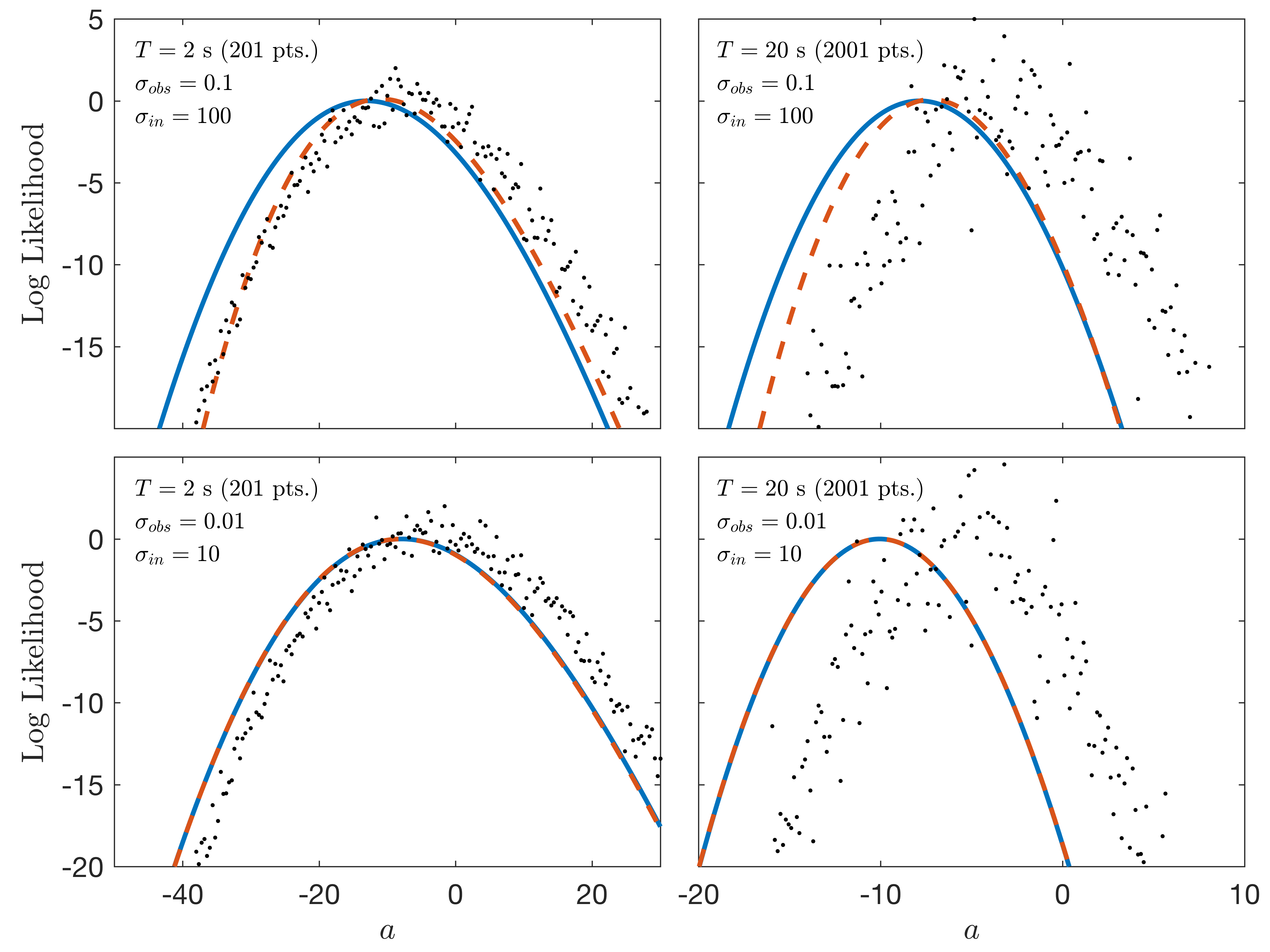
Figure 2: Comparison between Kalman filter (solid blue line), EKF (dashed red line) and particle filter (black dots) for the stochastic FitzHugh-Nagumo model. $P(t)$ is white noise with variance $\sigma_{in}^{2}$, observation noise with variance $\sigma_{out}^{2}$ is added. The only unknown parameter is $a$. The marginal likelihood is estimated on a uniformly spaced sequence of 200 $a$ values. Fixed parameters: $b=6000$, $c=40$, $d=4000$, $I_{0}=100$, $I(t)\equiv 0$. Time-step in solver and Kalman filter = $10^{-3}$, in observations = $10^{-2}$. Number of particles = $1000$.

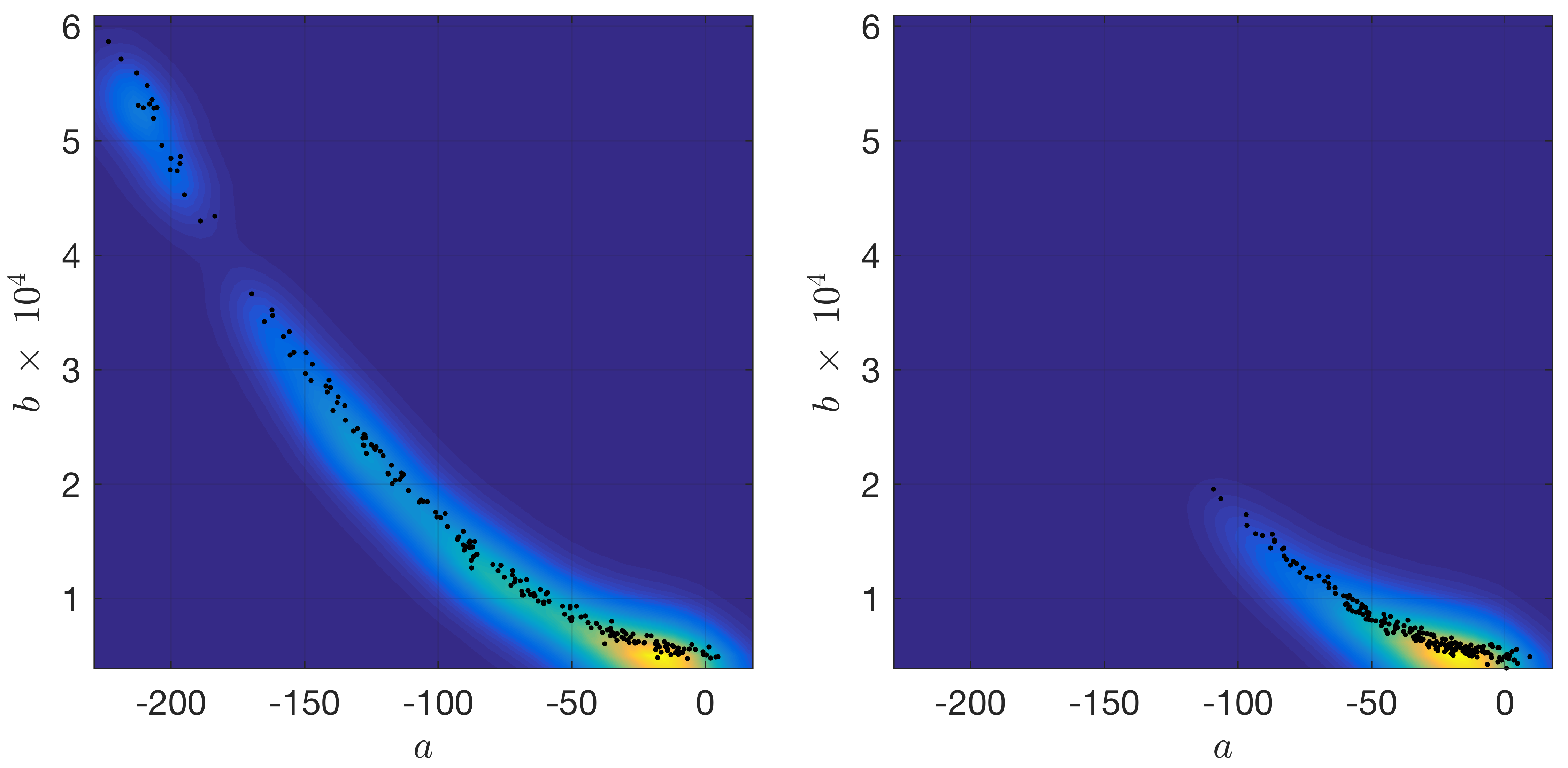
Figure 3: Comparison between marginal MCMC with Kalman filter (left) and EKF (right) on a problem with unknown parameters ($a$, $b$, $c$, $I_{0}$). Plots show MCMC samples from the joint $(a,b)$ marginal distribution only. Parameter values: $d=4000$, $T=2$, $\sigma_{in}=10$, $\sigma_{obs}=0.01$. Time-step in solver and Kalman filter = $10^{-3}$, in observations = $10^{-2}$. The MCMC chain started at the true parameters and ran for 10,000 iterations. Plots shows every 500th sample (black dots) and a smoothed histogram (coloured background).

Figure 2 shows that the error in the posterior is lower when the input noise and the observation noise are smaller. (We decrease both the noise parameters so that the signal to noise ratio does not change.) More specifically the Kalman filter and the EKF results are almost identical in the low noise setting, at least for the one-dimensional problem. The level of input noise controls the component of the error that comes from linearizing the model around a single point in the state-space, as opposed to linearizing locally around current state estimates (as in the EKF). The residual error, which exists when any form of linearization is done, is found by comparing the EKF with the particle filter. As is well known from previous studies, the EKF produces biased parameter estimates. Measured relative to posterior variance, the bias increases as more data is collected, see Figure 2. However, measured relative to the true parameter value, the bias in the posterior mean is small. Figure 2 also shows that larger data-sets result in larger variances for particle filter estimates for a fixed number of particles, an issue that is discussed in Kantas et al. (2015). This reinforces the message in Sec. 2.3 that the number of particles needed to effectively apply particle MCMC makes the algorithm intractable for many problems of practical interest. Figure 3 shows that accuracy on one-dimensional problems does not necessarily imply accuracy in higher-dimensional problems with the same model. The true parameters in this case correspond to the bottom-left panel in Figure 2, i.e., the input noise is sufficiently low that the Kalman filter and EKF are almost identical in one dimension. For the higher dimensional problem (where $a$, $b$, $c$, $I_{0}$ are all unknown), we see that the Kalman filter over-estimates uncertainty, although it still captures the qualitative dependencies in the posterior.

4 Analysis using Neural Population Model

Here we consider a problem from neuroscience that is extremely computationally expensive using particle MCMC, and where application of the Whittle likelihood makes a significant difference to computational efficiency compared to the Kalman filter. The use of the Whittle likelihood, enabled by linearizing about the fixed point, leads to a reduction in computational cost of a factor of 100 compared to the Kalman filter and several more orders of magnitude compared to particle MCMC. This approximation yields an algorithm that runs in several hours, compared to several months when using the EKF instead.

Other methods based on spectral analysis, similar to the Whittle likelihood, are currently used in EEG data analysis (Moran et al., 2009; Pinotsis et al., 2012a; Abeysuriya and Robinson, 2016). These methods have the same computational complexity as the Whittle likelihood. The reason for choosing the Whittle likelihood over these alternative spectral analysis methods is the theoretical support outlined in Sec. S2.3.3. This makes it possible to analyse the expected accuracy of the Whittle likelihood. In particular, we are able to estimate how long the time-series should be in order to make the bias introduced by the Whittle likelihood negligible. As far as we are aware, this type of analysis is absent from the neuroscience methodology papers that combine modelling and spectral analysis. We also test whether the model reparameterization makes a difference when applied within the smMALA algorithm (Algorithm 2 in the Supplement). We find a similar improvement in MCMC efficiency as when the reparameterization was applied within the MwG algorithm for the FitzHugh-Nagumo equations in Sec. 3.1.

In Secs. S4.1 and S4.2 of the Supplement, we describe in detail the Neural Population Model (NPM) that we would like to infer the parameters of, and explain how the reparameterization method can be applied to this model. For reference, the model employed here consists of the following DEs, where $l=e,i$ for excitatory and inhibitory contributions:

$$\tau_{l}\frac{d}{dt}h_{l}(t) =h_{l}^{r}-h_{l}(t)+\sum_{k=e,i}\frac{h_{kl}^{eq}-h_{l}(t)}{|h_{kl}^{eq}-h_{l}^{r}|}I_{kl}(t),$$ (23)

$$\left(\frac{1}{\gamma_{el}}\frac{d}{dt}+1\right)^{2}I_{el}(t) =q_{el}\left\{N^{\beta}_{el}S_{e}(t)+\Phi_{el}(t)+\bar{p}_{el}+\delta_{el}\ p(t)\right\},$$ (24)

$$\left(\frac{1}{\gamma_{il}}\frac{d}{dt}+1\right)^{2}I_{il}(t) =q_{il}N^{\beta}_{il}S_{i}(t),$$ (25)

$$\left(\frac{1}{v\Lambda}\frac{\partial}{\partial t}+1\right)^{2}\Phi_{el}(t) =N^{\alpha}_{el}S_{e}(t),$$ (26)

$$S_{k}(t) =S_{k}^{max}/\left\{1+\exp\left[\frac{\bar{\mu}_{k}-h_{k}(t)}{\hat{\sigma}_{k}/\sqrt{2}}\right]\right\},$$ (27)

where the Kronecker delta $\delta_{el}$ admits only excitatory noise input $p$ to this SDE system.

In modeling the EEG with this NPM, one typically assumes that the EEG observations are linearly proportional to $h_{e}$ with some added observational noise. We hence assume the following observation model,

$$y_{i}=h_{e}(i\cdot\Delta t)+n_{i}$$ (28)

where $\Delta t$ is some constant time-step and the $n_{i}$ are i.i.d. normal random variables, for $i=0,\ldots,n-1$. Figure S5 in the Supplement shows typical pseudo-data and spectral densities obtained with this model. Here we will be interested in the parameters governing the local reaction to incoming synaptic inputs ($\gamma_{ee}$, $\gamma_{ei}$, $\gamma_{ie}$, $\gamma_{ii}$, $q_{ee}$, $q_{ei}$, $q_{ie}$, and $q_{ii}$), which are commonly influenced by psychoactive substances and thus of considerable practical importance. We will assume the other parameter values are known, and simulate data from the model with a specific parameter set in order to test our statistical methodology, i.e., we will rely on pseudo-data for the following analysis.

The NPM introduced above has several different dynamical regimes, e.g., quasi-linear around a stable fixed point, limit cycles, or chaotic. Our working assumption is that if the data is weakly stationary, the underlying process can be modelled with parameter values leading to approximately linear dynamics around a stable fixed point for this NPM. See Sec. 3.2 for a detailed discussion of the effect of linearization. For the FitzHugh-Nagumo model we found that using the marginal likelihood calculated with the linearized model resulted in a posterior distribution that over-estimated uncertainty. The same may be true for the NPM, although it is more difficult to test because of the greater computational resources required to run the Kalman filter, extended Kalman filter and particle filter. We have simulated the model at parameter sets sampled by the MCMC algorithm and found a good agreement between nonlinear and linearized behaviour, consistent with the results in Bojak and Liley (2005).

4.1 Results

For this problem, particle MCMC is not computationally tractable, so we cannot make a direct comparison of the different likelihood choices. Below we present MCMC results for parameter estimation in the NPM with approximately linear dynamics. We use the Whittle likelihood and the smMALA algorithm (Algorithm 2). Here the Whittle likelihood is over 100 times faster than the Kalman filter. This is so because there is only one non-zero input, and we only observe one system state, so the likelihood calculation is faster by a factor of $O(d^{2})$ with here $d=14$. Following the discussion in Sec. S3.2, we use the definition of $\phi$ in Eq. (14) and the heuristic in Eq. (13) to determine the minimum time series length for which we expect the Whittle likelihood to be accurate. For this model, the theoretical spectral density $f(\nu_{k};\theta)$ for parameters $\theta$ is calculated using the method in Sec. S2.2 and the autocovariance function can be calculated numerically

$$\gamma_{xx}(h\cdot\Delta t)=\sum_{k=0}^{n-1}f(\nu_{k};\theta)e^{i2\pi kh/n}.$$ (29)

Assuming the parameters of Tab. S1 in the Supplement, the result of this analysis is a minimum time series length of around $7,000$ time-points, which is equivalent to around 14 s of data. For this particular model we found that the smMALA algorithm had better convergence than the MwG algorithm (Algorithm 1). We ran the MwG algorithm for a long time from a random initialisation and it did not sample parameter values close to the true parameter set (results not shown).

We chose a product of independent log-normal distributions as the prior distribution for the model parameters. See Sec. S4.3 in the supplementary material for more details. The smMALA algorithm was run on data simulated from a known parameter set, referred to as the true parameters. The parameter set used to initialize the MCMC was generated by random sampling with a procedure that was blind to the true parameter values. The algorithm parameters were as follows: Langevin step-size $h=0.3$, number of MCMC iterations $=100,000$ and burn-in length $=20,000$. Table 3 compares the performance of the smMALA algorithm with the original parameterization against the performance with the reparameterization. The reparameterized model has a lower computational cost per MCMC iteration, and a higher ESS. The cost per iteration is lower because the parameters that are updated deterministically in the reparameterization are explicit function of the stochastically updated parameters. In the original parameterisation the steady-state were defined implicitly, and a nonlinear solver was required to obtain their values given the other parameters. Reparameterizing the model may also have reduced nonlinearities in the likelihood function, leading to the higher ESS. The overall gain in efficiency is around a factor ten for Langevin step-size $h=0.3$. Table 3 also shows the results for a smaller value of the step-size parameter, $h$, in smMALA. In this case the two parameterizations have similar acceptance rates. An explanation for the difference in results for different $h$ values is that for the higher $h$ value the discretization of the Langevin diffusion is unstable in a large region of the parameter space for the original parameterization, but not for the reparameterized model. In contrast, for the lower $h$ value the discretization is stable over most of the parameter space in both parameterisations of the model.

empty

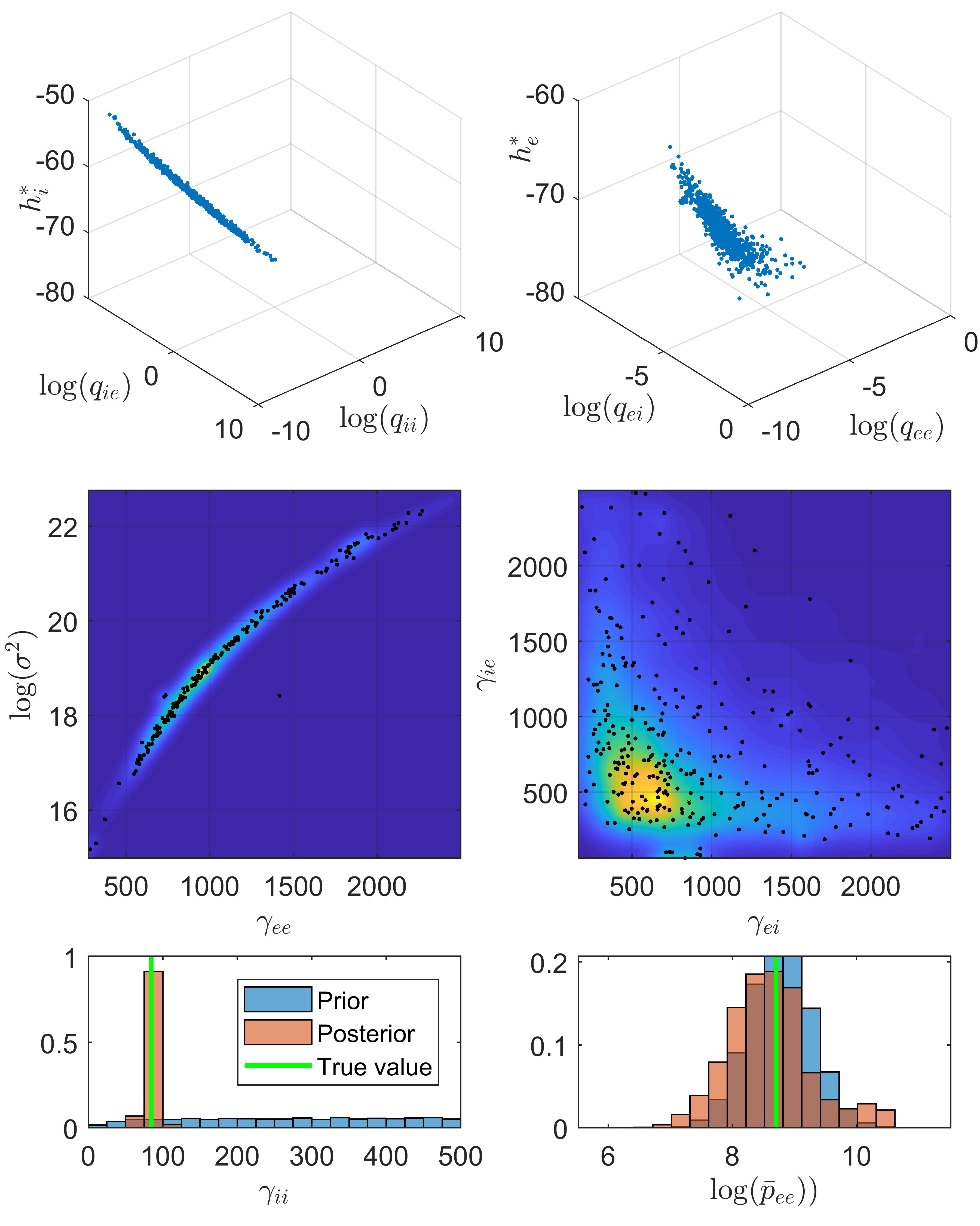
Figure 4: MCMC results with smMALA algorithm for reparameterized Neural Population Model with reparameterization. See Tab. S1 in the Supplement for the true parameter values, and Sec. 4.1 for algorithm parameters.

Figure 4 shows samples obtained from the smMALA algorithm with the reparameterization. The algorithm was initialized from a randomly generated initial parameter set. After around 2,000 iterations, the sampler finds a region of the parameter space with approximately the same likelihood as the true parameters. The algorithm samples close to the true parameter values for some of the time, but the range of parameter sets sampled in regions of high likelihood is relatively wide, indicating weak identifiability and/or non-identifiability of the model parameters. The samples generated from the smMALA algorithm confirm previous results obtained from sensitivity analysis (Bojak and Liley, 2005), which found that the model is more sensitive to the value of $\gamma_{ii}$ than to other parameter values, see our Figure 4. More interestingly, the samples can be used to identify previously unknown relationships between parameter values in the model. For example, there is strong negative correlation between the $h_{i}$ steady-state value and $q_{ii}$, which is proportional to the total charge transferred at synapses between inhibitory neurons, see Figure 4.

	Acceptance rate	CPU time per iteration	Mean ESS	$h$
Original parameterization	34%	5.66s	36	0.3
Reparameterization	69%	3.18s	239	0.3
Original parameterization	76%	5.66s	23	0.1
Reparameterization	74%	3.18s	34	0.1

Table 3: Comparison of MCMC with and without model reparameterization for smMALA algorithm on NPM. See Sec. 4.1 for algorithm parameters. The parameter $h$ is the step-size in the smMALA algorithm.

5 Discussion

Whilst parameter estimation for ODEs and SDEs is a well-studied problem in statistics, there has been little work on tailoring inference techniques to the case where the system operates close to a stable equilibrium point. An exception to this is the work contained in Meerbach (2009). Our work is different from this in that we retain the ability to infer mechanistic parameters of the system, thus retaining interpretability of model inferences.

This paper exploits the mathematical structure that is present in quasi-linear dynamics around a stable equilibrium. We have found that a reparameterization of the parameter space around an equilibrium point results in significantly improved efficiency of MCMC algorithms, and that linearizing the system about the stable equilibrium point yields a model that approximates the posterior distribution found from the corresponding nonlinear model.

This approximation can result in a reduction in computation cost of several orders of magnitude, a welcome boon for any application and a necessary condition for some to achieve practical feasibility. For example, EEG data for a single subject may consist of $50-100$ time series, each containing 1-2 million data-points. For the data in this paper, the particle MCMC we ran on a time series of length $200$, took over a month to run (in R). Although this may have been speeded up significantly using the most recent algorithmic and computational methods in the literature, it is still orders of magnitude slower than would be required to run on real data. Even the much cheaper EKF is not feasible for fitting a sophisticated model such as that in Sec. 4, where the dimension of the state space results in costly matrix inversions at every iteration of the filter. Our approach avoids these computationally expensive steps. Compared to the EKF approach, the effect of the linearization about a fixed point vanishes as the input noise decreases, and the effect of the Whittle approximation vanishes as the length of the time series increases. Outside of these situations, our approach tends to over-estimate posterior uncertainty, but captures the qualitative dependency between parameters well. Since our approach overestimates uncertainty, it is well suited to being used to speed up an exact approach such as importance sampling or delayed acceptance (these approaches are being compared in Vihola et al. (2016)).

In addition to the central idea of exploiting the properties of the stable equilibrium point, we have introduced two additional innovations that we expect to be more widely useful. Firstly, we have presented the methodology for using gradient based methods with the Whittle likelihood for linear SDEs (which may also be used in maximum likelihood estimation). Secondly, we introduce an easy to calculate diagnostic for assessing when the Whittle likelihood is likely to be appropriate.

Whilst the methods in this paper are suitable when the model only has a single stable equilibrium point, or if the system stays close to only one specific equilibrium point during observations, they can be inaccurate when this condition is not satisfied. We have shown that it is possible to determine whether the linearization methods are accurate without having to do a full posterior inference using exact methods. The FitzHugh-Nagumo system is often used as an example of a simple system that exhibits complicated nonlinear behaviour, and for this system one can construct cases where our proposed linearization is not appropriate. For such situations, when particle MCMC is infeasible, alternative approximate inference techniques are required. Such methods might build on the work in this paper through the use of a local Whittle approximation (such as that in Everitt et al. (2013)).

Supplementary material

S1 Introduction

This supplement contains mathematical detail and derivations, pseudo-code of the MCMC algorithms, as well as discussions of additional results only briefly summarized in the main paper.

S2 Methodology

S2.1 Model reparameterization

If the dimensions of $\mathbf{F}$ and $\mathbf{\theta}_{d}$ do not coincide, e.g., if in our application a background input is added only to some equations of the system, then the equilibrium calculation can be split as follows

$$\mathbf{F}_{1}[\mathbf{x}^{*},\theta_{s}] =0,$$ (S1)

$$\mathbf{F}_{2}[\mathbf{x}^{*},\mathbf{\theta}_{s}]+\mathbf{\theta}_{d} =0,$$ (S2)

where $\mathbf{F}=(\mathbf{F}_{1},\mathbf{F}_{2})$, and now $\mathbf{F}_{2}$ and $\mathbf{\theta}_{d}$ have the same dimension, i.e., in our application only these equation receive background inputs. The previous Eq. (4) then is the special case of $\mathbf{F}_{1}=\emptyset$. Now the model can be reparametrised in terms of $(\mathbf{\theta}_{s},\mathbf{x}_{2}^{*})$, where $\mathbf{x}^{*}=(\mathbf{x}_{1}^{*},\mathbf{x}_{2}^{*})$ and $\mathbf{x}_{2}^{*}$ has the same dimension as $\mathbf{\theta}_{d}$. Please note that while $\mathbf{F}_{1}$ and $\mathbf{x}_{1}^{*}$ have the same number of dimensions, as do $\mathbf{F}_{2}$ and $\mathbf{x}_{2}^{*}$, the partitioning of state components can differ between $\mathbf{F}$ and $\mathbf{x}^{*}$, since we can freely choose which components of $\mathbf{x}^{*}$ to trade for the $\mathbf{\theta}_{d}$. We can write our solutions as

$$\mathbf{x}_{1}^{*} =\mathbf{G}_{1}[\theta,\mathbf{x}_{2}^{*}],$$ (S3)

$$\mathbf{\theta}_{d} =\mathbf{G}_{2}[\theta_{s},\mathbf{x}^{*}]=\mathbf{G}_{2}[\theta_{s},(\mathbf{G}_{1}[\theta_{s},\mathbf{x}_{2}^{*}],\mathbf{x}_{2}^{*})]\equiv\tilde{\mathbf{G}}_{2}[\theta_{s},\mathbf{x}_{2}^{*}],$$ (S4)

Note that we assume only that a solution can be obtained numerically, where $\mathbf{G}_{1}$ is the solution corresponding to $\mathbf{F}_{1}$, and $\mathbf{G}_{2}$ to $\mathbf{F}_{2}$, respectively. The number of unknowns and the number of constraining equations is the same as in the original equations for the steady-state: $\mathrm{dim}(\mathbf{x}_{1}^{*})+\mathrm{dim}(\theta_{d})=\mathrm{dim}(\mathbf{x}^{*})=\mathrm{dim}(\mathbf{F})$. If the solutions in Eqs. (S3)-(S4) can be obtained in closed form by algebraically re-arranging the equations, then this obviously has practical advantages. This will be the case for the examples we consider in the main paper. In this case given $(\theta_{s},\mathbf{x}_{2}^{*})$ through an MCMC update, we can compute $(\mathbf{x}_{1}^{*},\theta_{d})$ directly by substitution into known formulae.

When and why might a reparameterization be effective? Consider sampling from a complex target distribution with an MCMC algorithm where the proposal does not take account of the covariance structure in the target distribution (such as the Metropolis-within-Gibbs algorithm in supplementary Sec. S2.4). The steady-state can be a complex function of several elements of $\theta$, and the likelihood is often very sensitive to the steady-state. This leads to strong correlations in the likelihood. If the dependencies between elements of $(\theta_{s},\mathbf{x}_{2}^{*})$ are weaker than the dependencies between elements of $\mathbf{\theta}$, then it will be easier to sample on the reparametrised space than on the original space. The reparameterization method can also be useful in MCMC algorithms that do take account of the covariance structure in the target distribution (such as the simplified manifold MALA algorithm in supplementary Sec. S2.4). If the equilibrium point is a nonlinear function of the model parameters, then this may cause the target distribution to have non-constant curvature. In the reparameterization, $\mathbf{\theta}_{d}=\tilde{\mathbf{G}}_{2}[\theta_{s},\mathbf{x}_{2}^{*}]$ will be a nonlinear function. If the likelihood is more sensitive to $\mathbf{x}_{2}^{*}$ than it is to $\mathbf{\theta}_{d}$, then we would expect sampling on the reparametrised space to be more efficient: the gain in efficiency is obtained by reducing nonlinearity in the likelihood function.

Prior distributions may be specified on the original parameter space. In this case, if we are proposing parameters on the reparametrised space, we need to evaluate a Jacobian determinant in order to correctly evaluate the prior density in the MCMC acceptance ratio,

$$p(\theta_{s},\mathbf{x}^{*}_{2})=p(\theta_{s},\theta_{d})\ |\mathcal{J}_{\mathbf{T}}|,\ \mathrm{where}\ \mathbf{T}:(\theta_{s},\mathbf{x}_{2}^{*})\rightarrow(\theta_{s},\theta_{d})=(\theta_{s},\tilde{\mathbf{G}}_{2}[\theta_{s},\mathbf{x}_{2}^{*}]).\\$$ (S5)

The Jacobian determinant, $|\mathcal{J}_{\mathbf{T}}|$, can be evaluated analytically if $\tilde{\mathbf{G}}_{2}$ is available in closed form. If not, $|\mathcal{J}_{\mathbf{T}}|$ can be approximated numerically using finite differences (yielding a noisy MCMC algorithm (Alquier et al., 2016), not considered further in this paper).

Examples of applying the reparameterization method, along with further specific explorations of its effectiveness, can be found in Secs. 3 and 4 of the main paper. However, we want to draw attention to two further issues that are relatively common in practice. First, it is possible that the map $\theta\rightarrow\mathbf{x}^{*}$ is not well-defined because there are multiple stable equilibria for one given set of parameters $\theta$. In this case the following map is still well-defined for stable ODEs: $(\theta,\mathbf{x}_{0})\rightarrow\mathbf{x}^{*}$, where $\mathbf{x}_{0}$ is the initial condition of the system. For SDEs with multiple stable equilibria, there is always a positive probability that the system will jump between the basins of attraction of the different stable states. The methods presented in this paper are theoretically not applicable in this setting. However, in practice the system may remain close to one specific stable state during the entire interval when the observations, $y$, are collected. If so, then it is possible to construct a map $(\theta,y)\rightarrow\mathbf{x}^{*}$ that is de facto well defined. The likelihood for this de facto mono-stability typically increases with a decrease of the strength of the noise driving the system. Second, the proposal densities $q[(\theta_{s},\theta_{d})\rightarrow(\mathbf{x}^{*}_{1},\mathbf{x}^{*}_{2})]$ and $\tilde{q}[(\theta_{s},\mathbf{x}_{2}^{*})\rightarrow(\mathbf{x}^{*}_{1},\theta_{d})]$ could have support on different regions of $\mathcal{R}^{d_{\theta}+d_{x}}$. For example, prior knowledge may dictate that for $\theta_{d}<0$ one has $q=0$ but this is not explicit in the reparametrised $\tilde{q}\neq 0$. If there is such strong prior information then more work needs to be done to ensure that $q$ and $\tilde{q}$ have the same support. For example, it may be that $\theta_{d}>0$ implies $\mathbf{x}^{*}_{2}>\mathbf{x}_{0}$. If so, then an appropriate $\tilde{q}[(\theta_{s},\mathbf{x}_{2}^{*})\rightarrow(\mathbf{x}^{*}_{1},\theta_{d})]$ would be a normal distribution on $\log[\mathbf{x}^{*}_{2}-\mathbf{x}_{0}]$.

S2.2 The spectral density of stable SDEs

S2.2.1 Linearization and the spectral density

In Sec. 2.3 we describe several different methods for approximating the likelihood in stable SDEs. In this section, we introduce two key tools that are needed for the faster likelihood calculations. The first tool is linearization. To linearize the model, we apply a Taylor approximation to the right-hand side of Eq. (1)

$$\mathbf{F}[\mathbf{x};\theta]\approx\mathbf{F}[\mathbf{x}^{*};\theta]+\mathcal{J}(\mathbf{x}^{*};\theta)(\mathbf{x}-\mathbf{x}^{*}),$$ (S6)

where $\mathcal{J}(\mathbf{x}^{*},\theta)$ is the Jacobian evaluated at $\mathbf{x}^{*}$ with parameters $\theta$. The accuracy of linearization depends on the size of the higher order derivatives of $\mathcal{J}$, and on the size of $\delta\mathbf{x}\equiv\mathbf{x}-\mathbf{x}^{*}$. We are seeking to apply linearization around a stable equilibrium $\mathbf{F}[\mathbf{x}^{*};\theta]=0$. The size of $\delta\mathbf{x}$ will then depend on the size of $\mathbf{p}(t;\theta)$, which is the term that pushes the system away from its equilibrium:

$$\frac{d}{dt}\delta\mathbf{x}(t)=\mathcal{J}(\mathbf{x}^{*};\theta)\ \delta\mathbf{x}(t)+\mathbf{p}(t;\theta),$$ (S7)

The effect of this approximation on inference was explored in Sec. 3.2 of the main paper.

The second tool is a spectral density calculation. This is useful for performing inference in the frequency domain, e.g., evaluation of the Whittle likelihood. If $x_{j}(t)$ is the $j\/$-th component of the multivariate stochastic process $\mathbf{x}(t)$, then the (power) spectral density of $x_{j}(t)$ is

$$S_{xx}^{j}(\nu)=\frac{1}{T}\left|X_{j}^{T}(\nu)\right|^{2},$$ (S8)

i.e., the spectral density is proportional to the squared modulus of $X_{j}^{T}(\nu)$, where $X^{T}_{j}(\nu)$ denotes the Fourier transform of $x_{j}^{T}(t)$. Here $x_{j}^{T}(t)$ is $x_{j}(t)$ with support on the interval $\left[-\frac{T}{2},\frac{T}{2}\right]$, i.e., with $x_{j}^{T}(t)=0$ outside of this interval. In principle Eq. (S8) is to be understood in a $\lim_{T\rightarrow\infty}$ sense, but in practice $T$ corresponds to the actual length of the data and one obtains an estimate. To simplify the notation we will drop the component index $j$ and the interval superscript $T$ in the following. The Fourier transform is defined only up to choices in constant factors and naming conventions (Weisstein, 1999-2017):

$$x(\beta)=\sqrt{\frac{|b|}{(2\pi)^{1+a}}}\int_{-\infty}^{\infty}d\alpha\,X(\alpha)e^{-ib\alpha\beta}\quad\mathrm{and}\quad X(\alpha)=\sqrt{\frac{|b|}{(2\pi)^{1-a}}}\int_{-\infty}^{\infty}dt\,x(\beta)e^{ib\alpha\beta}.$$ (S9)

In Eq. (S8) we have implicitly used $(a,b,\alpha,\beta)=(0,-2\pi,\nu,t)$, which is common in applications. For this choice the Fourier variable $\alpha$ corresponds to the ordinary frequency $\nu$.

Assuming a weakly stationary process mean-zero process, and here setting $\beta=\tau$ as is convention for the lag variable, the Wiener-Khinchin theorem then can be written as

$$\gamma_{xx}(\tau)=\mathrm{E}\left[x(t+\tau)x(t)\right]=\int_{-\infty}^{\infty}d\nu\ S_{xx}(\nu)e^{i2\pi\nu\tau},$$ (S10)

i.e., the spectral density is simply the Fourier transform of the autocovariance. Typically one assumes that the difference between the (discretely sampled) process and the observations is a stochastic process, such as white noise. When two processes $x(t)$ and $z(t)$ are independent, then the autocovariance of $y(t)=x(t)+z(t)$ is simply $\gamma_{yy}(\tau)=\gamma_{xx}(\tau)+\gamma_{zz}(\tau)$. It follows from Eq. (S10) that then also $S_{yy}(\nu)=S_{xx}(\nu)+S_{zz}(\nu)$. If $z(t)$ is zero-mean white noise, then $\gamma_{zz}(\tau)=\sigma^{2}\delta(\tau)$ with variance $\sigma^{2}$ and Dirac $\delta(t)$, and consequently the measured spectral density will have a “noise floor” $S_{yy}(\nu)=S_{xx}(\nu)+\sigma^{2}$. The connection to the discrete (time) Fourier transform required for analysing experimental data is straightforward, using $\Delta t=T/n$ and $\Delta\nu=1/T$:

$$x\left(t=t_{l}\equiv l\cdot\Delta t\right) \quad\longrightarrow\quad x_{l}=\frac{1}{\sqrt{n}}\sum_{k}X_{k}e^{i2\pi kl/n},$$ (S11)

$$X\left(\nu=\nu_{k}\equiv k\cdot\Delta\nu\right)/\Delta t \quad\longrightarrow\quad X_{k}=\frac{1}{\sqrt{n}}\sum_{l}x_{l}e^{-i2\pi kl/n},$$ (S12)

$$S_{xx}\left(\nu=\nu_{k}\equiv k\cdot\Delta\nu\right)/\Delta t \quad\longrightarrow\quad S_{k}=|X_{k}|^{2},$$ (S13)

where $k,l=-\frac{n}{2}+1,..,\frac{n}{2}$, or $k,l=0,...,n-1$ with the explicit $n\/$-periodicity in the discrete case.

The Fourier transform of a system of linear SDEs can be evaluated as follows, where we will be using the Fourier choice common in mathematics $(a,b,\alpha,\beta)=(1,-1,\omega,t)$ to avoid extraneous “$2\pi$” factors. Any system of linear differential equations can be written in the form

$$\frac{d}{dt}\mathbf{x}(t)=\mathcal{A}\,\mathbf{x}(t)+\mathbf{p}(t),$$ (S14)

cf. Eq. (S7). Using integration by parts, the Fourier transform of $d\mathbf{x}/dt$ is

$$\int_{-\infty}^{\infty}dt\ \left(\frac{d}{dt}\mathbf{x}(t)\right)e^{-i\omega t} =\bigg{[}\mathbf{x}(t)e^{-i\omega t}\bigg{]}_{t=-\infty}^{t=\infty}-\int_{-\infty}^{\infty}dt\ \mathbf{x}(t)\left(\frac{d}{dt}e^{-i\omega t}\right)$$

$$=i\omega\mathbf{X}(\omega).$$ (S15)

Applying the Fourier transform also to the other side of Eq. (S14) we obtain

$$\left(i\omega\mathbb{1}-\mathcal{A}\right)\mathbf{X}(\omega)=\mathbf{P}(\omega).$$ (S16)

For a given value of $\omega$, Eq. (S16) is a linear system of equations, which can be re-arranged to obtain $\mathbf{X}(\omega)$ as a function of $\mathbf{P}(\omega)$. The matrix $\mathcal{T}(\omega)$ that maps $\mathbf{P}(\omega)$ to $\mathbf{X}(\omega)$ is called the transfer function

$$\mathbf{X}(\omega)=\mathcal{T}(\omega)\ \mathbf{P}(\omega).$$ (S17)

An expression for $\mathcal{T}(\omega)$ can be obtained using the eigen-decomposition of $\mathcal{A}$ (Bojak and Liley, 2005):

$$\mathcal{T}(\omega)=\mathcal{R}\ \mathrm{diag}\bigg{[}\frac{1}{e_{k}(i\omega-\lambda_{k})}\bigg{]}\ \mathcal{L},$$ (S18)

where the $j\/$-th column of $\mathcal{R}$ is the $j\/$-th right-eigenvector of $\mathcal{A}$, the $i\/$-th row of $\mathcal{L}$ is the $i\/$-th left-eigenvector, $\lambda_{1},\ldots,\lambda_{k},\ldots,\lambda_{d}$ are its eigenvalues, and $e_{1},\ldots,e_{k},\ldots,e_{d}$ are norms of the eigenvectors obtained from $\mathcal{L}\mathcal{R}=\mathrm{diag}[e_{k}]$.

This derivation provides us with an important observation: the computational complexity of evaluating the spectral density can be reduced if only some of the elements of the transfer function matrix are needed. In the examples in this paper only one element of $\mathbf{x}(t)$ is observed, and only one element of the input $\mathbf{p}(t)$ is assumed to be non-zero. This means that only a single element of the transfer function matrix needs to be calculated. Thus, by exploiting sparsity in both the assumed input to the system and its measured output, the complexity of evaluating the spectral density is reduced to $O(N\,d)$, with $N$ the number of points where the spectral density is being evaluated and $d$ the dimension of the state-space. This implies significant computational savings compared to the worst case $O(N\,d^{3})$ where all elements of $\mathbf{x}(t)$ and $\mathbf{p}(t)$ are needed. Such sparsity in input-output components is quite common in scientific applications, since one one hand often experimentally only one or a small number of state variables of the system are accessible, and on the other hand experiments are often designed to disentangle inputs (e.g., a task provides highly specific excitation or observations are made when a certain inputs are known to be dominant).

Other straightforward ways of improving the efficiency of such spectral density calculations are

• reducing the frequency resolution, e.g., by decimation or window-averaging;

• setting the spectral density to zero above a known frequency threshold of the system; and

• parallelizing the computation of the $d^{2}$ entries of $\mathcal{T}(\omega)$.

Use of the first two of techniques is problem-dependent, and care needs to be taken to ensure that the bias introduced is negligible. The results here can be easily extended to calculate cross-spectral densities. This is useful for problems where multiple components of the process are observed.

S2.2.2 Derivatives of the spectral density

Some parameter estimation algorithms, such as Metropolis Adjusted Langevin Algorithm (MALA) require the likelihood to be differentiated. In order to apply such algorithms to likelihoods based on the spectral density, it is necessary to differentiate the spectral density. Derivatives can be approximated using finite differences. However, these can be time-consuming to compute, and inaccurate. Furthermore, the step-size in the finite difference approximation can only be decreased to a certain extent before rounding errors occur due to the limited machine precision. Here we derive analytic derivatives for the spectral density. The results are only valid when all eigenvalues of the system are distinct. In the problems we have looked at this condition is satisified for most of the parameter space, but not all of it. It is always possible to fall back on finite differences, if parameter sets with repeated eigenvalues are sampled.

The derivatives of the spectral density can be used to evaluate analytic derivatives of the Whittle likelihood for stable SDEs as follows, where we indicate the derivative by the parameters $\theta$ as subscript. Note that the parameters themselves are real, not complex.

$$TS_{xx,\theta}(\omega)=\frac{\partial}{\partial\theta}\left|\mathbf{X}(\omega)\right|^{2}=\left\{\frac{\partial}{\partial\theta}\left[\Re^{2}\mathcal{T}(\omega)+\Im^{2}\mathcal{T}(\omega)\right]\right\}\left|\mathbf{P}(\omega)\right|^{2}+\left|\mathcal{T}(\omega)\right|^{2}\left\{\frac{\partial}{\partial\theta}\left[\Re^{2}\mathbf{P}(\omega)+\Im^{2}\mathbf{P}(\omega)\right]\right\}$$

$$=2\left\{\left[\Re\mathcal{T}(\omega)\Re\mathcal{T}_{\theta}(\omega)+\Im\mathcal{T}(\omega)\Im\mathcal{T}_{\theta}(\omega)\right]\left|\mathbf{P}(\omega)\right|^{2}+\left|\mathcal{T}(\omega)\right|^{2}\left[\Re\mathbf{P}(\omega)\Re\mathbf{P}_{\theta}(\omega)+\Im\mathbf{P}(\omega)\Im\mathbf{P}_{\theta}(\omega)\right]\right\}$$ (S19)

To evaluate the derivatives of $\mathcal{T}(\omega)$, we need the derivatives of the eigenvalues and eigenvectors (Giles, 2008). Differentiating both sides of $\mathcal{J}\mathbf{r}=\lambda\mathbf{r}$ gives us,

$$\mathcal{J}_{\theta}\mathbf{r}+\mathcal{J}\mathbf{r}_{\theta}=\lambda_{\theta}\mathbf{r}+\lambda\mathbf{r}_{\theta},$$ (S20)

where $\mathcal{J}_{\theta}$ means each element of the Jacobian matrix $\mathcal{J}$ is differentiated with respect to $\theta$, and likewise for the right eigenvector $\mathbf{r}$ and $\mathbf{r}_{\theta}$. We require that right eigenvectors have unit length, i.e., $\mathbf{r}^{T}\mathbf{r}=1$. Differentiating this constraint with respect to $\theta$ yields

$$\mathbf{r}^{T}\mathbf{r}_{\theta}=0.$$ (S21)

Combining Eqs. (S20) and (S21), and re-arranging, we obtain,

$$\left[\begin{array}[]{c|c}\mathcal{J}-\lambda\mathbb{1}&-\mathbf{r}\\ \hline\cr\mathbf{r}^{T}&0\\ \end{array}\right]\left[\begin{array}[]{c}\mathbf{r}_{\theta}\\ \hline\cr\lambda_{\theta}\\ \end{array}\right]=\left[\begin{array}[]{c}-\mathcal{J}_{\theta}\ \mathbf{r}\\ \hline\cr 0\\ \end{array}\right].$$ (S22)

This is a $(d+1)\times(d+1)$ linear system, which we can solve for $(\mathbf{u}_{\theta},\lambda_{\theta})$. Furthermore, if we want to calculate derivatives with respect to $p$ different parameters, we can calculate the inverse of the matrix on the left-hand side, which is an $\mathcal{O}(d^{3})$ operation, and use this matrix to calculate the $p$ derivatives. Overall the computational complexity is then $\mathcal{O}(d^{3}+pd^{2})$. The cubic complexity here is manageable in the regime we are interested in, i.e., when $p,d\approx 10-50$. In general the rate-limiting steps in our calculations are those that involve a factor of $n$, as $n>10^{4}$.

When $p$ and $d$ are both on the order of $10-100$ or greater, this means we get approximately a factor of $d$ saving compared to the finite difference approach, which evaluates the eigenvalues and eigenvectors separately for each of the $p$ parameters. A similar calculation can be done for left eigenvectors, $\mathbf{l}^{T}\mathcal{J}=\lambda\mathbf{l}^{T}$, and the computational saving is the same:

$$\mathbf{l}^{T}_{\theta}\left(\mathcal{J}-\lambda\mathbb{1}\right)=-\mathbf{l}^{T}\left(\mathcal{J}_{\theta}-\lambda_{\theta}\mathbb{1}\right).$$ (S23)

Note that we assume here that $\lambda_{\theta}$ has already been computed in the right eigenvector case. Furthermore, we require the cross-norm $\mathbf{l}^{T}\mathbf{r}=1$, i.e., $\mathcal{L}\mathcal{R}=\mathrm{diag}[e_{k}]=\mathbb{1}$. This removes any further parameter dependence from $\mathcal{T}(\omega)$. For second derivatives, we can simply differentiate Eqs. (S20) and (S21) again, to obtain another $(d+1)\times(d+1)$ linear system. This time the second derivatives of the eigenvectors and eigenvalues are the unknowns. In this case the overall computational complexity for calculating the second derivatives with respect to $p$ different parameters is $\mathcal{O}(d^{3}+p^{2}d^{2})$, compared to $\mathcal{O}(p^{2}d^{3})$ for the finite difference calculation. Once the eigenvector and eigenvalue derivatives have been obtained it is straightforward to differentiate $\mathcal{T}(\omega)=\mathcal{R}\ \mathrm{diag}[1/(i\omega-\lambda_{k})]\ \mathcal{L}$. In the worst-case scenario when all elements of $\mathcal{T}(\omega)$ are needed, this has a computational complexity of $\mathcal{O}(p\,n\,d^{3})$ for first derivatives. In the best-case scenario where only one element is needed, it is $\mathcal{O}(p\,n\,d)$. Differentiating with respect to the parameters of the input process, $\mathbf{P}(\omega)$, is straight-forward because the parameters values in $\mathbf{P}(\omega)$ do not affect the eigen-decomposition of $\mathcal{J}$.

S2.3 Marginal likelihoods for indirectly observed SDEs

S2.3.1 Particle filter

If we discretize an SDE, and assume that observations are a sample path plus some observation noise, we obtain a state-space model. The solutions to SDEs and state-space models are samples from a probability distribution over an appropriate space. To simplify the notation we write the distribution explicitly only in the finite-dimensional state-space case. The marginal likelihood of $y_{1:n}$, conditional on $\theta$ is,

$$p_{\theta}(y_{1:n})=p_{\theta}(y_{1})\prod_{i=2}^{n}p_{\theta}(y_{i}|y_{1:i-1})$$ (S24)

where

$$p_{\theta}(y_{i}|y_{1:i-1})=\int g_{\theta}(y_{i}|x_{i})f_{\theta}(x_{i}|x_{i-1})p_{\theta}(x_{1:i-1}|y_{1:i-1})\,dx_{1:n}$$ (S25)

Particle filters combine importance sampling and resampling to obtain Monte Carlo estimates of the integral in Eq. (S25) for $i$ from $2$ to $n$. In the simplest form of the particle filter, the importance sampling proposal is $f_{\theta}(x_{i}|x_{i-1})\hat{p}_{\theta}(x_{1:i-1}|y_{1:i-1})$, and the importance weights are $g_{\theta}(y_{i}|x_{i})$. The resampling uses the normalized weights as probabilities of a discrete distribution. The distribution $\hat{p}_{\theta}(x_{1:i-1}|y_{1:i-1})$ is a sum of equally weighted Dirac delta-functions centred on the resampled particles. If we use $N$ particles to estimate the integrals in Eq. (S25), the overall cost of the estimate is $O(Nnd)$, where $d$ is the dimension of the state-space. Depending on the problem and the variant of particle filter used, $N$ may be somewhere in the range 100-10,000. Outside of special cases where we may simulate exactly from the SDE dynamics, this approach yields a biased approximation to the likelihood due to discretization error. If we wish for a better approximation to the SDE, we may sample paths on a finer grid than the observations, which increases the computational cost of the particle filter.

S2.3.2 Kalman filter

If the SDE or state-space model is linear then $f_{\theta}(x_{i}|x_{i-1})$ is a Gaussian distribution. If we further assume that the likelihood of observations $y_{1:n}$ conditional on $x_{1:n}$ is a product of Gaussians, then the probability distributions inside the integral of Eq. (S25) are all Gaussian, and the Kalman filter can be used to evaluate the marginal likelihood analytically. This has a computational cost of $O(nd^{3})$. Again the cost is higher if we sample paths on a finer grid than the observations. We note that in the ODE case, where there is no uncertainty in the $x_{1:n}$ conditional on $\theta$, the likelihood simplifies to the evaluation of a multivariate Gaussian, with computational cost $O(nd)$:

$$p_{\theta}(y_{1:n})=\prod_{i=1}^{n}p\left[y_{i}|x_{\theta}(t_{i})\right]=\prod_{i=1}^{n}\mathrm{N}\left[x_{\theta}(t_{i}),\sigma_{o}^{2}\right].$$ (S26)

The standard approach to linearizing a non-linear dynamic system is the extended Kalman filter (EKF), where a linearization of the dynamics is performed at each iteration of the filter, setting the transition matrix to be the Jacobian evaluated at the current state estimate. There are some applications where this approximation is known to be inadequate, leading to the divergence of the filter. However, in practice this approximation is often suitable, and the method is widely used. In this paper we propose to use an approximation that is less widely applicable, but which we show can lead to very computationally efficient algorithms. Namely, we propose to use a single linearization of the dynamics, about the stable equilibrium point of the model (as described in the supplementary Sec. S2.2). This yields a single transition matrix to be used at every iteration of the Kalman filter. Although this approximate model is usually less accurate than the EKF, as alluded to in Sec. 1.1, the additional approximation can be small (as has been exploited in computational neuroscience, e.g., in Moran et al. (2009); Pinotsis et al. (2012b); Abeysuriya and Robinson (2016)).

S2.3.3 Whittle likelihood

In the remainder of this section we briefly recall the derivation of the Whittle likelihood, following Shumway and Stoffer (2011). We will refer to this in Sec. S3.2 of the Supplement, where we study the accuracy of this approximation. We assume that the process has zero mean, but it is not difficult to generalize the Whittle likelihood to the non-zero case. As defined above, the periodogram of a time series is the squared modulus of its Discrete Fourier Tranform (DFT)

$$S_{k}=|X_{k}|^{2} =\left|\sum_{l}x_{l}e^{-i2\pi kl/n}\right|^{2}$$

$$=\left[\frac{1}{\sqrt{n}}\sum_{l}x_{l}\cos\frac{2\pi kl}{n}\right]^{2}+\left[\frac{1}{\sqrt{n}}\sum_{l}x_{l}\sin\frac{2\pi kl}{n}\right]^{2}$$

$$=X_{k}^{c\;2}+X_{k}^{s\;2}.$$ (S27)

with the the discrete cosine and sine transforms. If the time series $x_{l}$ is a normal random variable with mean zero, then as linear combinations also $X_{k}^{c}$ and $X_{k}^{s}$ will be jointly normal with mean zero. Using $f(\nu)\equiv S_{xx}(\nu)/\Delta t$ and $\nu_{k}=k\cdot\Delta\nu=k/(n\Delta t)$, the variances and covariances are as follows (Shumway and Stoffer, 2011):

$$\mathrm{Cov}[X_{k}^{c},X_{l}^{c}] =\frac{f(\nu_{k})}{2}\delta_{kl}+\epsilon_{n}$$ (S28)

$$\mathrm{Cov}[X_{k}^{s},X_{l}^{s}] =\frac{f(\nu_{k})}{2}\delta_{kl}+\epsilon_{n}$$ (S29)

$$\mathrm{Cov}[X_{k}^{c},X_{l}^{s}] =\epsilon_{n},$$ (S30)

with Kronecker $\delta_{kl}$. Here $|\epsilon_{n}|<\phi/n$, and

$$\phi=\sum_{h=-\infty}^{\infty}|h|\left|\gamma_{xx}(h\cdot\Delta t)\right|,$$ (S31)

where $\gamma_{xx}(\tau)$ is the autocovariance function defined in Sec. S2.2.1 of the supplementary material.

The Whittle likelihood is obtained by dropping the $\epsilon_{n}$ terms. This eliminates the dependence between $X_{k}^{c}$ and $X_{k}^{s}$ as well as the bias in the remaining terms. The sum of the squares of two independent standard normal random variables is a $\chi^{2}$ distribution with two degrees of freedom, hence

$$p_{\theta}(x_{0},\ldots,x_{n-1})=p_{\theta}(S_{0},\ldots,S_{n-1})\approx\prod_{k=1}^{n/2-1}\frac{1}{f(\nu_{k};\theta)}\exp\left[-\frac{S_{k}}{f(\nu_{k};\theta)}\right],$$ (S32)

where we now have made explicit the dependence on model parameters $\theta$ and, as is common, neglected the mean and Nyquist spectral edges $k=0,n/2$. Note that the terms $S_{n/2},\ldots,S_{n-1}$ do not appear in the product since they are are fully determined by $S_{1},\ldots,S_{n/2-1}$ for real signals. The equation $|\epsilon_{n}|<\phi/n$ tells us that the error in the approximation decreases linearly with $n$, and also that it depends on the decay rate of the autocovariance function. The effect of the error on inference, and how this varies with $\phi$ and $n$ is analysed in Sec. S3.2 of the Supplement. It is straightforward to extend the derivation above to obtain an Whittle likelihood for observations $p_{\theta}(y_{0},\ldots,y_{n-1})$, if the system state $\mathbf{x}_{i}$ is indirectly observed according to Eq. (10) and independent from the “observation noise” $\mathbf{n}_{i}$.

S2.4 MCMC algorithms

Input: Data, $y$; Initial value for $\theta=(\theta_{1},\ldots,\theta_{p})$;
Likelihood $l(y|\theta)$; Prior distribution $p(\theta)$.

Proposal variances, $\sigma^{2}_{1}$,…,$\sigma^{2}_{p}$; Number of iterations, $I$ for $i=2,\ldots,I$  do

       for $j=1,\ldots,p$ do

             Propose $\theta^{*}_{j}\sim N(\theta_{j},\sigma^{2}_{j})$;

             Evaluate acceptance ratio, $\alpha(\theta,\theta^{*})=\mathrm{min}\left[1,\dfrac{l(y|\theta^{*})p(\theta^{*})}{l(y|\theta)p(\theta)}\right]$;

             Draw $u\sim\mathrm{Uniform}(0,1)$;

             if $u<\alpha(\theta,\theta^{*})$ then Set $\theta=\theta^{*}$ ;

            

       end for

      

end for

Algorithm 1 Metropolis-within-Gibbs (MwG)

Input: Data, $y$; Initial value for $\theta=(\theta_{1},\ldots,\theta_{p})$;
Likelihood $l(y|\theta)$; Prior distribution $p(\theta)$.

Step size, $h$; Number of iterations, $I$ for $i=2,\ldots,I$  do

       Evaluate gradient and Hessian of the unnormalized log posterior,
$g=\nabla\bigg{[}\log[\ l(y|\theta)\ p(\theta)\ ]\bigg{]}$ and $H_{\theta}$;

       Set $C=h^{2}H_{\theta}^{-1}$, and $m=\theta+\frac{1}{2}C\,g$;

       Propose $\theta^{*}\sim q(\theta^{*}|\theta)=N(m,C)$;

       Evaluate acceptance ratio, $\alpha(\theta,\theta^{*})=\mathrm{min}\left[1,\dfrac{l(y|\theta^{*})p(\theta^{*})q(\theta|\theta^{*})}{l(y|\theta)p(\theta)q(\theta^{*}|\theta)}\right]$;

       Draw $u\sim\mathrm{Uniform}(0,1)$;

       if $u<\alpha(\theta,\theta^{*})$ then Set $\theta=\theta^{*}$ ;

      

end for

Algorithm 2 Simplified manifold Metropolis Adjusted Langevin Algorithm (smMALA)

In this paper we use two standard MCMC algorithms: Metropolis-within-Gibbs (MwG), and the simplified manifold Metropolis Adjusted Langevin Algorithm (smMALA) (Girolami and Calderhead, 2011). Pseudo-code for these are provided as Algorithms 1 and 2. The MwG algorithm is easier to implement. The smMALA gives a higher Effective Sample Size (ESS) because the proposal uses the local gradient and Hessian of the posterior. The smMALA requires more computational resources per iteration because of the gradient and Hessian calculations. If the posterior has a relatively simple geometry, the cost of the gradient and Hessian calculations may outweigh the benefits of a better proposal. An accessible presentation of the smMALA algorithm along with application to a brain imaging problem can be found in Penny and Sengupta (2016). In all cases the algorithm can be implemented with the original model parametrisation or with the steady-state reparametrisation outlined in Sec. 2.1. In Secs. 3 and 4, we will demonstrate how using the steady-state reparametrisation can lead to more efficient sampling of the parameter space. When using the Langevin method, we calculate the gradient of the Whittle likelihood using the analytic derivatives of the spectral density derived in Sec. S2.2. In later sections, we use the term marginal MCMC as a label for MCMC algorithms where the likelihood $l(y|\theta)$ is a marginal likelihood that is calculated analytically, e.g., using a Kalman filter.

S3 Analysis using the FitzHugh-Nagumo equations

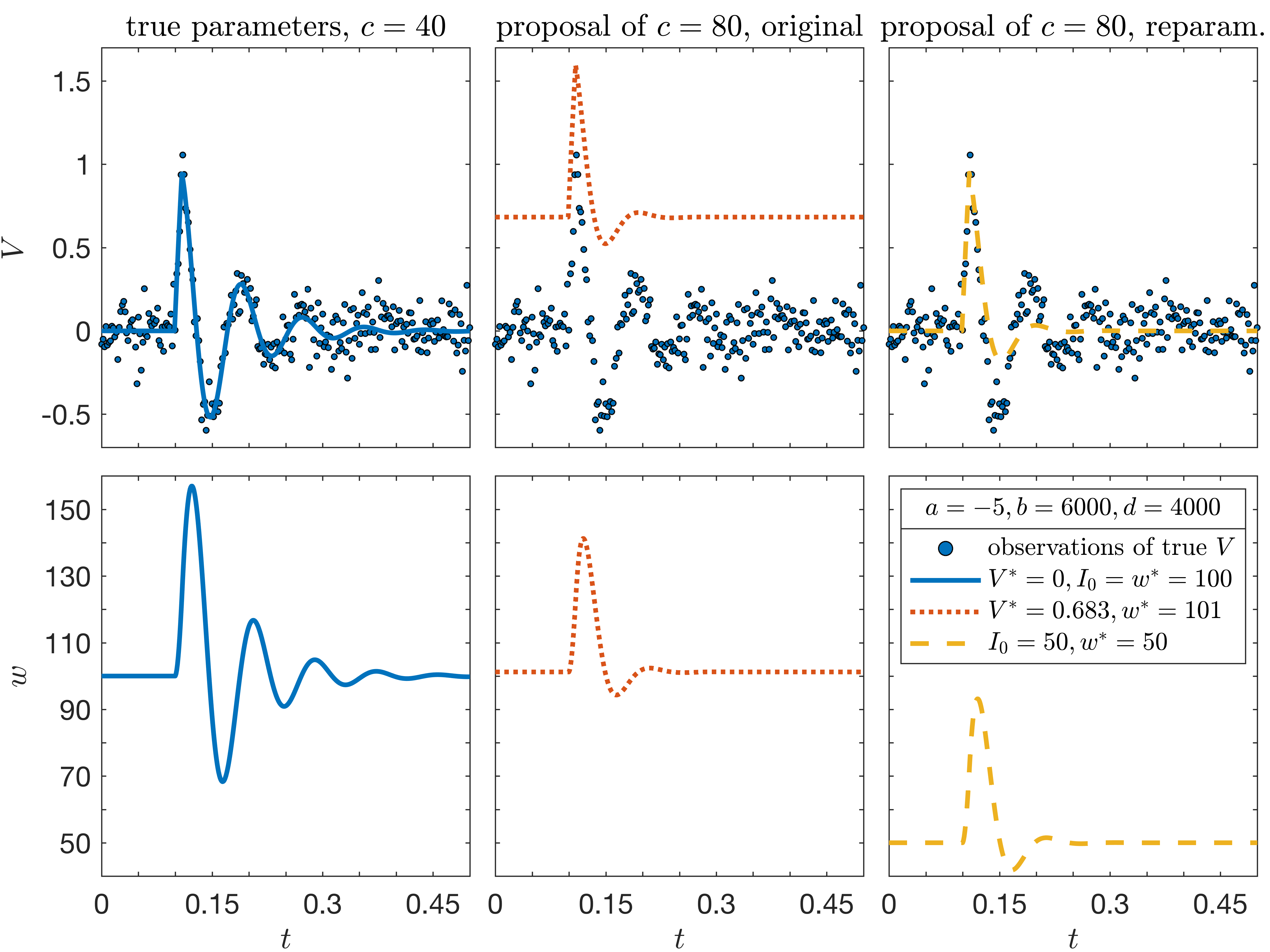
Figure S1: Reparameterization example. Left column: Solutions (blue solid lines) for $V$ (top) and $w$ (bottom) for $a=-5$, $b=6000$, $d=100$, $c=40$, $I_{0}=100$. Noisy observations of this $V$ (blue dots) are shown here and in the other columns. Middle column: A proposal with $c=80$ (other parameters identical) changes $(V^{*},w^{*})$. The solution (orange dotted line) deviates strongly from the observations. Right column: The same proposal in the reparametrised scheme (golden dashed line) changes $(I_{0},w^{*})$. Since $V^{*}=0$ remains unchanged, deviations remain limited.

S3.1 Results for deterministic FitzHugh Nagumo equations

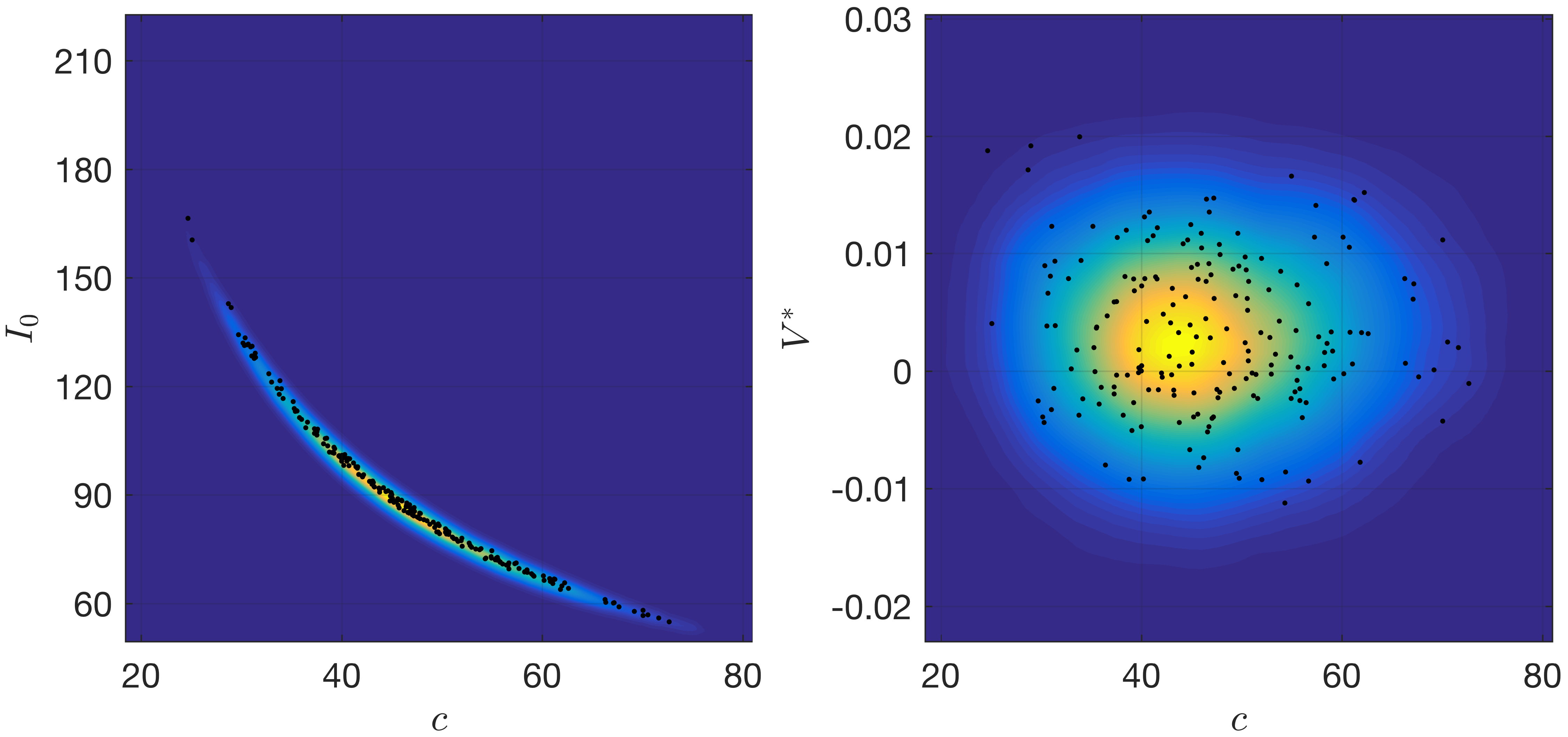
Figure S2: MCMC results for deterministic FHN. The posterior correlation between $c$ and $V^{*}$ (right panel, reparametrised) is much weaker than the correlation between $c$ and $I_{0}$ (left panel, original). The MCMC chain was started at the true parameter set ($a=-5$, $b=6000$, $c=40$, $I_{0}=100$) and run for 100,000 iterations. Every 500th sample (black dots) and a smoothed histogram (background colour map) are shown. Quantiles (0.025, 0.5, 0.975) of posteriors for parameters not shown were $a$: (-11, 4.11, 15.4) and $b$: (4980, 5400, 6250).

Here we set $P(t)=0$ throughout, but $I(t)=100$ for the time interval $1<t<1.1$ and $I(t)=0$ otherwise. The initial conditions are set to the stable equilibrium. This is a function of the model parameters, so the initial conditions change when the parameters are updated. It would not be difficult to extend the methods here to the case when the model parameters and the initial conditions are treated as separate parameters of the inference problem. The numerical solution and parameter values used are shown in Fig. S1, along with numerical solutions at two other parameter sets. We make the following assumptions about the inference problem: (i) we can only observe $V$ with observation noise, and do not have any observations for $w$, (ii) the value of $d$ is known, (iii) The prior distributions for $a$, $b$, $c$, $I_{0}$ are uniform over a large (unspecified) range.

Scatterplots for selected pairs of parameters and table summaries of the posterior distribution (obtained using the reparametrised algorithm) are shown in Figure S2.

Figure S1 illustrates how the likelihood of the data is sensitive to the steady-state value $V^{*}$. This induces strong correlations in the posterior distribution between the original model parameters, $c$ and $I_{0}$, seen in Figure S2. Reparameterizing the likelihood using the steady-state value results in a likelihood function with weaker correlations (Figure S2). This means that that the MwG algorithm should be able to sample the parameter space more efficiently. A Metropolis-within-Gibbs MCMC algorithm (Algorithm 1) was run with and without model reparameterization. In both cases, the parameters are updated using a Gaussian distribution centred on the current parameter value. The proposal width was tuned manually using preliminary runs with a procedure that estimates the conditional standard deviation in the posterior distribution (Raftery and Lewis, 1995). This resulted in different proposal widths between the two parametrisations. We evaluated the performance of each MCMC algorithm by estimating the Effective Sample Size (ESS) for each parameter using the LaplacesDemon package in R. There is a wide range in the ESS values across parameters. This is because some parameters are largely independent of the other parameters (leading to a high ESS). However there are also strongly correlated parameter pairs (leading to a low ESS). When the model is reparametrised the minimum ESS is around 14 times higher than it is with the original parametrisation; the same is true of the average ESS (see Tab. 2).

It is worth noting that the difference in the ESS is not the same for all parameter sets. Indeed there are some scenarios where the ESS decreases for some of the parameters when the model is reparameterized (not shown). It is also worth noting that the ESS in the reparametrised model is still only a small fraction of the number of MCMC iterations, around $0.1-0.5\%$. These observations suggest that even when the model is reparamterised, the MCMC mixes relatively slowly. Depending on the model and computational resources available this may or may not be a problem. If it is problematic, as we have found to be the case for the Neural Population Model considered later, then algorithms based on Langevin or Hamiltonian dynamics may perform better. If the mixing rate is not problematic, MwG with reparameterization offers an easy to implement alternative to Langevin and Hamiltonian Monte Carlo methods. Since MwG does not require costly derivative calculations, there may also be situations when the overall computational efficiency is higher (as measured by ESS / CPU-time).

S3.2 Comparison between Kalman filter and Whittle likelihood on linear model

This section continues the analysis of the Whittle likelihood accuracy. We compare the Whittle likelihood with the Kalman filter in a situation where the Kalman filter is exact up to discretization error. The linear model that we use is derived by linearizing the FHN equations around a stable fixed point. As mentioned above, for $d=I_{0}=0$ in Eqs. (15) and (16), the system will always have an equilibrium at $(V^{*},w^{*})=(0,0)$. As in the previous section, we assume here that $I(t)=0$ and $P(t)$ is white noise. If we are only interested in $v(t)=V(t)-V^{*}$ we can eliminate $w(t)-w^{*}$ from the linearized model to obtain a driven harmonic oscillator

$$\left(\frac{d^{2}}{dt^{2}}+2\zeta\omega_{0}\frac{d}{dt}+\omega_{0}^{2}\right)v(t)=P(t),$$ (S33)

where $2\zeta\omega_{0}\equiv a+c$ and $\omega_{0}^{2}\equiv ac+b$. Note that the conditions for obtaining a stable equilibrium point mentioned above then become $2\zeta\omega_{0}>0$ and $\omega_{0}^{2}>0$. Without loss of generality, we hence can choose $\omega_{0}>0$ for the natural frequency and then require $\zeta>0$ for the damping to obtain stability. Eq. (S33) is equivalent to what is sometimes referred to as the continuous parameter AR(2) process (Priestley, 1981). The spectral density for the harmonic oscillator, driven by white noise, is a single peak if the oscillator is sufficiently under-damped $\zeta<1/\sqrt{2}$. The location of the spectral peak is $\omega_{1}=2\pi\nu_{1}=\omega_{0}\sqrt{1-2\zeta^{2}}$.

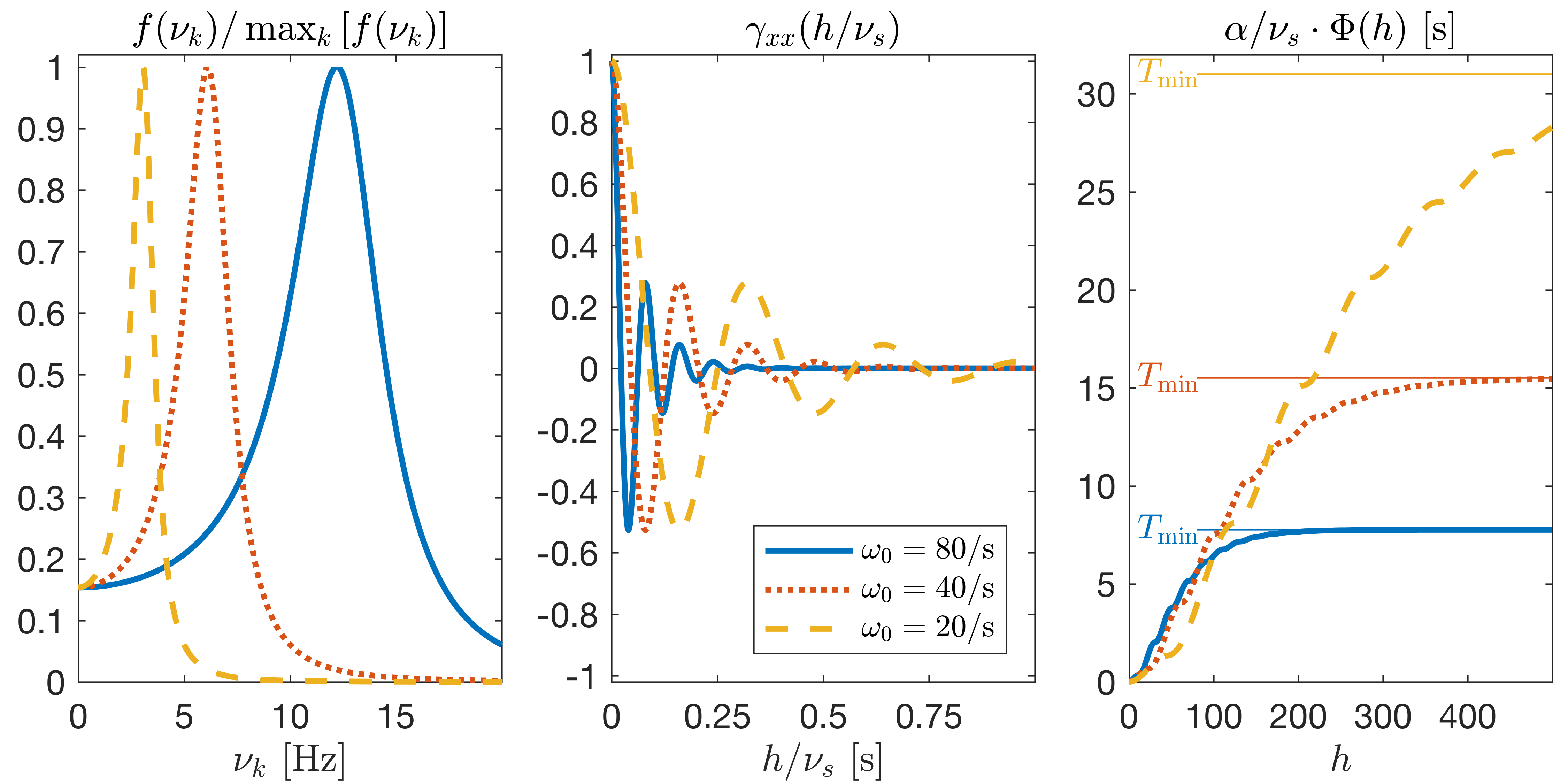
Figure S3: Normed spectral density (left), autocovariance (middle), and accuracy heuristic (right) for the harmonic oscillator with damping $\zeta=0.2$ and three different $\omega_{0}$: 80/s (blue solid lines), 40/s (dotted red lines), and 20/s (golden dashed lines). Sampling frequency $\nu_{s}=500\leavevmode\nobreak\ \mathrm{Hz}$. The minimum time-series length can be calculated using Eq. (13): $n_{\min}=\nu_{s}T_{\min}\equiv\alpha\phi=\alpha\lim_{h\rightarrow\infty}\Phi(h)$, where $\alpha\equiv(0.01\cdot\max_{k}\left[f(\nu_{k})\right])^{-1}$ and $\Phi(h)\equiv 2\sum_{j=0}^{h}|j||\gamma_{xx}(j/f_{s})|$. $T_{\min}$ values for the different $\omega_{0}$ are shown as thin lines in the right panel in matching colours.

In Sec. S3.2, we saw that the accuracy of of the Whittle likelihood depends on two quantities: $\phi$ given by Eq. (S31) and $n$, the length of the time series. Inspection of Eq. (S31) reveals that $\phi$ (and hence the error in the Whittle likelihood) is larger when the autocovariance is high at long lags, i.e., for strong correlations between time-points that are far away from each other in the discrete-time index. Further analysis has been done for the AR(1) process, (Contreras-Cristán et al., 2006), showing that a higher AR(1) coefficient (i.e., stronger correlation between time-points) lead to a larger error. For processes with a monotonically decaying autocovariance function it is clear that a slower decay in the autocovariance will mean that a longer time-series is needed to justify the use of the Whittle likelihood.

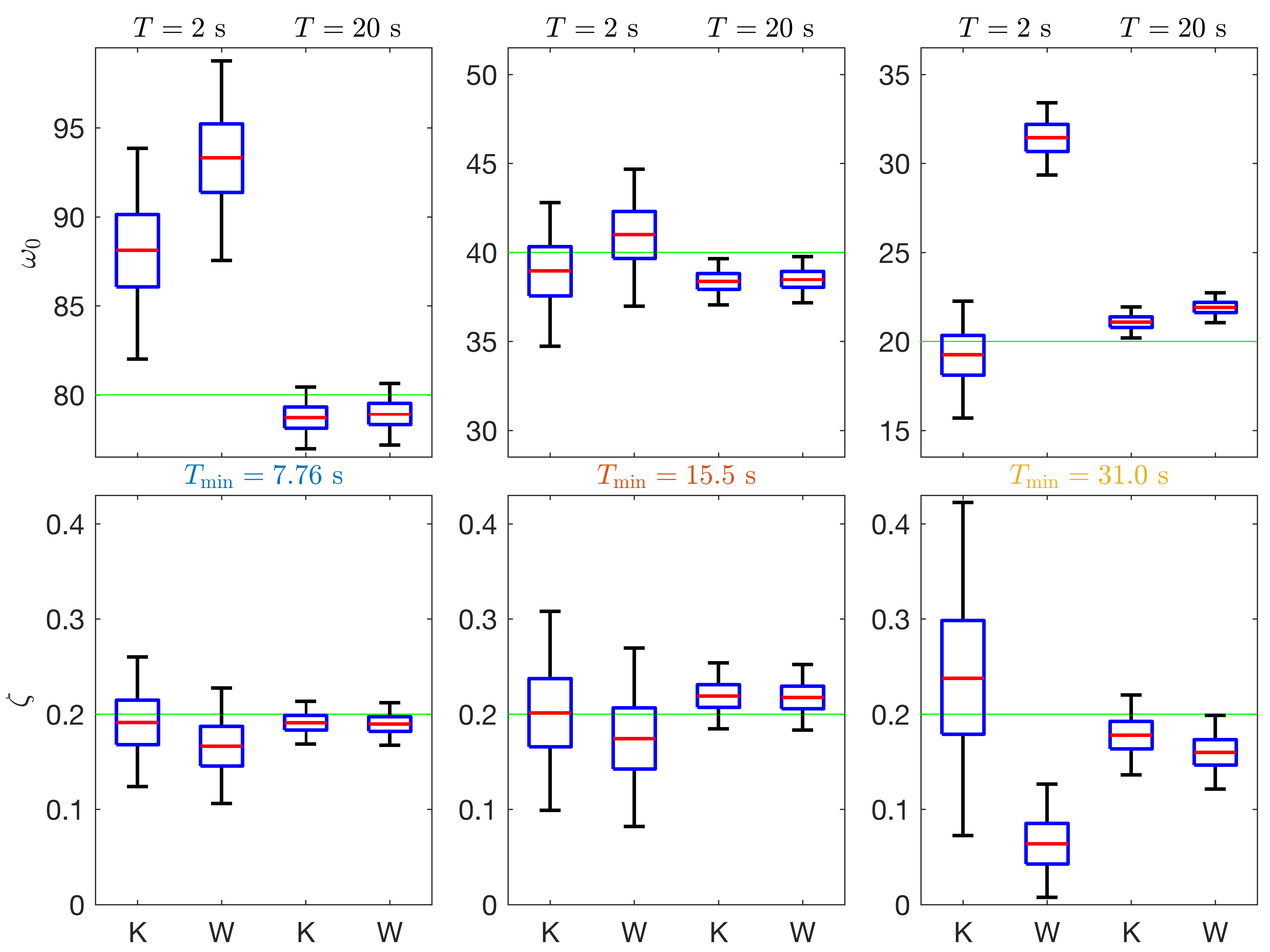
Figure S4: Boxplots of the marginal posterior distributions for $\omega_{0}$ (top) and $\zeta$ (bottom) under a uniform prior. The true parameters values are $\zeta=0.2$ (all plots), and $\omega_{0}=80,40,20/s$ (from left to right). The exact Kalman filter (K) and the approximate Whittle likelihood (W) analyses are in agreement only if $T\geq T_{\min}$, as predicted by the heuristic, Eq. (13), cf. Fig. S3 right.

In the case of oscillatory processes, such as the linearized stochastic FHN equations and the neural population model discussed in Sec. 4, the autocovariance function is oscillatory and decays to zero. There are then two distinct factors which affect the magnitude of $\phi$. First is the frequency of oscillations, or equivalently the location of resonance peak(s) in the spectral density. If the systems oscillates at a lower frequency this results in an autocovariance function with a longer period. Second is the regularity of the oscillations, or equivalently the width of the resonance peak(s) in the spectral density. If the frequency of oscillations is highly consistent over time, as opposed to being more spread across frequencies, this results in an autocovariance function that decays more slowly.

Further quantification of the error can be done by comparing likelihoods from the Kalman filter (which is exact up to discretization error) with the Whittle likelihood. For our purposes, the Whittle likelihood is accurate when the posterior distribution under the Whittle likelihood is similar to the posterior distribution under the Kalman filter. By numerical experimentation, we have found that the Kalman filter and Whittle likelihood posteriors are similar for the linearized FHN equations when

$$\frac{\phi}{n}<0.01\max_{k}\left[f(\nu_{k})\right].$$ (S34)

This is illustrated in Fig. S4. Since it is quicker to compute the quantity $\phi/n$ than to do a full comparison between posterior distributions, we recommend using Eq. (13) as a heuristic rule to decide whether the Whittle likelihood is a sufficiently accurate approximation to the true likelihood. For the example in the next section, estimating the posterior distribution using the Kalman filter is intractable and we rely on the heuristic in Eq. (13) to give an indication of whether the Whittle likelihood is accurate.

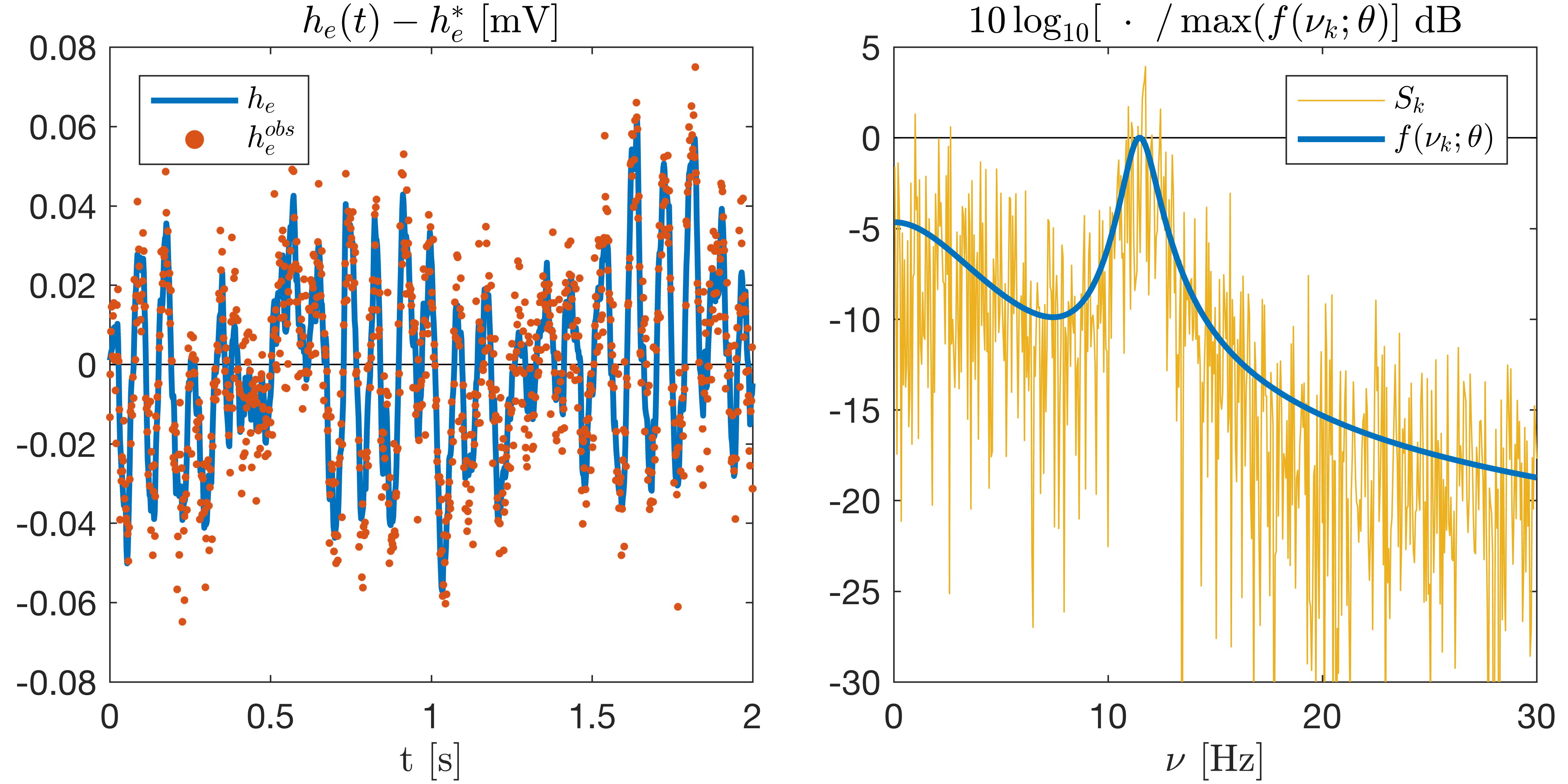
Figure S5: Left: First 2 s of $T=20$ s of pseudo-data generated with parameters from Tab. S1 as solid blue line, with noisy observations thereof as red dots. The (equilibrium) mean has been subtracted. Right: Decibel plot of spectral density of $T=20$ s observed pseudo-data (thin golden line) and predicted spectral density of linearized NPM model (thick blue line).

S4 Analysis using Neural Population Model

S4.1 Model description

The model in this section describes the mass action of neural tissue, rather than the activity of individual neurons. This class of models carries a variety of labels in the literature – usually called a “mass model” if discrete units of tissue are considered, but a “field model” if the tissue is modeled as a continuum. The model used here can represent either case, depending on how the activity propagation Eq. (S40) is specified, and we will use the generic label neural population model (NPM). We are interested in the neuroimaging problem of inferring NPM model parameters from EEG data. The characteristics of EEG datasets vary depending on the experimental setup and experimental subjects being studied. Event Related Potentials (ERPs) and epileptic seizure dynamics typically feature non-stationary and/or nonlinear behaviour (David et al., 2005; Andrzejak et al., 2001). In contrast, adult resting-state data can be considered as weakly stationary (Kreuzer et al., 2014) with a power spectrum that is a superposition of an inverse frequency (typically between $1/f$ and $1/f^{2}$) curve with a resonance peak in the so-called alpha range (8-13 Hz). Here we restrict ourselves to inferring the parameters when the true parameter values are static as opposed to time-varying.

Our NPM is known as the Liley model (Liley et al., 2002; Bojak and Liley, 2005), and it distinguishes two neural populations by their function: one excitatory, the other inhibitory. That distinction is made according to the effect neurons have on other neurons they are connected to. If the activity of the source neurons increases the activity of the target neurons, then they are excitatory, if it decreases it, inhibitory. The model can be split into three parts: dynamics of the mean soma membrane potentials ($h_{e}$ and $h_{i}$), local reaction to synaptic inputs ($I_{ee}$, $I_{ei}$, $I_{ie}$, and $I_{ii}$), and long-range propagation of activity ($\Phi_{ee}$ and $\Phi_{ei}$). In modeling the EEG with this NPM, one typically assumes that the EEG observations are linearly proportional to $h_{e}$ with some added observational noise.

The equations for the membrane potential dynamics are as follows,

$$\tau_{e}\frac{\partial}{\partial t}h_{e}(\mathbf{x},t) =h_{e}^{r}-h_{e}(\mathbf{x},t)+\psi_{ee}\left[h_{e}(\mathbf{x},t)\right]I_{ee}(\mathbf{x},t)+\psi_{ie}\left[h_{e}(\mathbf{x},t)\right]I_{ie}(\mathbf{x},t),$$ (S35)

$$\tau_{i}\frac{\partial}{\partial t}h_{i}(\mathbf{x},t) =h_{i}^{r}-h_{i}(\mathbf{x},t)+\psi_{ei}\left[h_{i}(\mathbf{x},t)\right]I_{ei}(\mathbf{x},t)+\psi_{ii}\left[h_{i}(\mathbf{x},t)\right]I_{ii}(\mathbf{x},t),$$

where

$$\psi_{kl}[h_{l}(\mathbf{x},t)]\equiv\frac{h_{kl}^{eq}-h_{l}(\mathbf{x},t)}{|h_{kl}^{eq}-h_{l}^{r}|}.$$ (S36)

The subscript $e$ stands for excitatory, $i$ for inhibitory, and $k$ and $l$ can take on either of these values. A single subscript denotes a quantity relating to a single neural population; whereas a double subscript denotes a quantity relating to the interaction between two populations, i.e., subscript $kl$ indicates $k$ acting on $l$. In the absence of synaptic inputs $I_{kl}$ the membrane potentials $h_{l}(\mathbf{x},t)$ will decay to rest values $h_{l}^{r}$ with characteristic times $\tau_{l}$. Synaptic inputs $I_{kl}\geq 0$ are weighted by the functions $\psi_{kl}$. Since for biological parameter ranges $h_{el}^{eq}>h_{l}^{r}$ but $h_{il}^{eq}<h_{l}^{r}$, at rest excitatory inputs $I_{el}$ are weighted by $+1$ but inhibitory ones $I_{il}$ by $-1$. Note that possibility of having zero weight or even a reversal of the sign, depending on the current state of the membrane potential, is not a mathematical artifact but reflects properties of voltage-gated ion channels.

The equations for local synaptic impact are

$$\left(\frac{1}{\gamma_{el}}\frac{\partial}{\partial t}+1\right)^{2}I_{el}(\mathbf{x},t) =q_{el}\left\{N^{\beta}_{el}S_{e}\left[h_{e}(\mathbf{x},t)\right]+\Phi_{el}(\mathbf{x},t)+p_{el}(\mathbf{x},t)\right\}$$ (S37)

$$\left(\frac{1}{\gamma_{ik}}\frac{\partial}{\partial t}+1\right)^{2}I_{ik}(\mathbf{x},t) =q_{ik}\left\{N^{\beta}_{ik}S_{i}\left[h_{i}(\mathbf{x},t)\right]\right\}$$

where

$$p_{ee}(\mathbf{x},t)=\bar{p}_{ee}+p(\mathbf{x},t),\qquad p_{ei}(\mathbf{x},t)=\bar{p}_{ei}\leavevmode\nobreak\ (\mathrm{const.})$$ (S38)

$$S_{k}\left[h_{k}(\mathbf{x},t)\right]=S_{k}^{max}/\left\{1+\exp\left[\frac{\bar{\mu}_{k}-h_{k}(\mathbf{x},t)}{\hat{\sigma}_{k}/\sqrt{2}}\right]\right\}.$$ (S39)

If the curly braces in Eqs. (S37) are replaced by a single Dirac delta distribution $\delta(t)$ representing one input spike, then one obtains as postsynaptic response canonical “alpha functions” $\gamma^{2}t\exp(-\gamma t)\Theta(t)$ weighted by $q$, where the indices have been left out for clarity and $\Theta(t)$ is the Heaviside step distribution. The terms in the curly braces hence represent counts for sources of such input spikes: local cortical firing $S_{k}$, firing propagated long-range in cortex $\Phi_{el}$ and extra-cortical input $p_{el}$ in particular from the thalamus.

The equations for the long-range propagation across cortex are

$$\left[\left(\frac{1}{v\Lambda}\frac{\partial}{\partial t}+1\right)^{2}-\frac{3}{2\Lambda^{2}}\nabla^{2}\right]\Phi_{ek}(\mathbf{x},t)=N^{\alpha}_{ek}S_{e}\left[h_{e}(\mathbf{x},t)\right]$$ (S40)

These equations correspond approximately to activity propagating isotropically outwards from firing sources $S_{e}\left[h_{e}(\mathbf{x},t)\right]$ with conduction velocity $v$, while decaying exponentially with a characteristic length scale $\Lambda$. Note that this would correspond to a “field model” in the terminology introduced at the beginning of this section. However, for simplicity we assume in what follows that the the system is spatially homogeneous, i.e., for the input $p_{ee}(\mathbf{x},t)\equiv p_{ee}(t)$ and likewise for all state variables. This describes coherent bulk oscillations of the brain. Then $\nabla^{2}\Phi_{ek}(\mathbf{x},t)\equiv 0$, and Eq. (S40) becomes a damped harmonic oscillator ODE without spatial dependence. Consequently, one can also interpret this as a “mass model” for a single unit of tissue. Alternatively, one can obtain a “mass model” by simply dropping Eq. (S40) entirely from the Liley model. However, the homogeneous “mass model” typically produces activity more similar to the “field model” for the same parameter values. The methodology developed in this paper can be applied to spatial models as well. See Bojak and Liley (2005) for details on how to evaluate the spectral density for spatially dependent solutions.

NPM knowns		NPM knowns		NPM unknowns		auxiliary
$\tau_{e}$	105.5 ms	$S^{max}_{e}$	355.2/s	$\gamma_{ee}$	841.2/s	sampling frequency
$\tau_{i}$	149.0 ms	$S^{max}_{i}$	424.8/s	$\gamma_{ei}$	859.7/s	$f_{s}$	500 Hz
$h^{r}_{e}$	-71.9 mV	$\bar{\mu}_{e}$	-52.3 mV	$\gamma_{ie}$	451.7/s
$h^{r}_{i}$	-76.0 mV	$\bar{\mu}_{i}$	-48.6 mV	$\gamma_{ie}$	451.7/s	recording duration
$h^{eq}_{ee}$	-9.0 mV	$\hat{\sigma}_{e}$	4.9 mV	$q_{ee}$	$0.9484\leavevmode\nobreak\ \mu\Omega\mathrm{C}$	$T$	20 s
$h^{eq}_{ei}$	-10.3 mV	$\hat{\sigma}_{i}$	3.7 mV	$q_{ei}$	$5.835\leavevmode\nobreak\ \mu\Omega\mathrm{C}$
$h^{eq}_{ie}$	-87.5 mV	$v$	780.7 cm/s	$q_{ie}$	$11.99\leavevmode\nobreak\ \mu\Omega\mathrm{C}$	std. dev. observation noise
$h^{eq}_{ii}$	-82.3 mV	$\Lambda$	0.345/cm	$q_{ii}$	$11.30\leavevmode\nobreak\ \mu\Omega\mathrm{C}$	$\sigma_{obs}$	0.01 mV
$N^{\beta}_{ee}$	2194	$N^{\alpha}_{ee}$	3668	$\bar{p}_{ee}$	6025/s
$N^{\beta}_{ei}$	4752	$N^{\alpha}_{ei}$	1033	$\bar{p}_{ei}$	1116/s	std. dev. noise input
$N^{\beta}_{ie}$	700					$\sigma_{p}$	100.0/s
$N^{\beta}_{ii}$	516

Table S1: List of NPM parameter values used to generate pseudo-data, taken from column 3 of Table 5 in Bojak and Liley (2005), as well as other parameters used in the simulation run. In the inference problem parameters labeled “NPM knowns” are assumed as given, i.e., only the “NPM unknowns” are being inferred from the pseudo-data.

For numerical calculations the noise input was treated with the Euler-Maruyama method, i.e., using independently generated Gaussian white noise in every time step

$$\ldots+h_{t}\cdot\bar{p}_{ee}+\frac{\sigma_{p}}{\sqrt{10^{-4}/s}}\sqrt{h_{t}}\cdot{\cal N}(0,1),$$ (S41)

where we have normed to the standard numerical time step $10^{-4}\leavevmode\nobreak\ \mathrm{s}$ for convenience in interpreting the noise standard deviation $\sigma_{p}$. Observations are made of the mean excitatory soma membrane potential $h_{e}$, and to simulate experimental measurement error we add independent Gaussian white noise with standard deviation $\sigma_{obs}$

$$h_{e}^{obs}(t_{k})=h_{e}(t_{k})+\sigma_{obs}\cdot{\cal N}(0,1).$$ (S42)

Here $t_{k}=k\cdot\Delta t$ with $k=0,\ldots,N-1$ indicates the discrete observations of the system. An illustration of the pseudo-data and predictions from this NPM is given in Fig. S5.

S4.2 Model reparameterization

For the NPM defined in Sec. S4.1, the equations of the form (S3) can be obtained by re-arranging the steady-state equations for short-range and long-range connectivity,

$$I^{*}_{ee} =q_{ee}\left[N^{\beta}_{ee}S_{e}(h_{e}^{*})+\Phi^{*}_{ee}+\bar{p}_{ee}\right],$$ (S43)

$$I^{*}_{ei} =q_{ei}\left[N^{\beta}_{ei}S_{e}(h_{e}^{*})+\Phi^{*}_{ei}+\bar{p}_{ei}\right],$$ (S44)

$$I^{*}_{ik} =q_{ik}\left[N^{\beta}_{ik}S_{i}(h_{i})\right],$$ (S45)

$$\Phi^{*}_{ee} =N^{\alpha}_{ee}S_{e}(h_{e}^{*}),$$ (S46)

$$\Phi^{*}_{ei} =N^{\alpha}_{ei}S_{e}(h_{e}^{*}).$$ (S47)

The remaining steady-state equations are,

$$0 =h_{e}^{r}-h^{*}_{e}+\psi_{ee}(h^{*}_{e})I^{*}_{ee}+\psi_{ie}(h^{*}_{e})I^{*}_{ie},$$ (S48)

$$0 =h_{i}^{r}-h^{*}_{i}+\psi_{ei}(h^{*}_{i})I^{*}_{ei}+\psi_{ii}(h^{*}_{i})I^{*}_{ii}.$$ (S49)

Equations $\eqref{eq:npmss_a}-\eqref{eq:npmss_c}$ can be used to eliminate $I^{*}_{ee}$, $I^{*}_{ei}$, $I^{*}_{ie}$, $I^{*}_{ii}$ from (S48)-(S49). The resulting equations are of the form (S4) with $\mathbf{x}^{*}_{2}=(h_{e}^{*},h_{i}^{*})$, and $\theta_{d}=(\bar{p}_{ee},\bar{p}_{ei})$. Note that the solutions for $\theta_{d}$ are easily obtained in closed form.

S4.3 Parameter values for prior distribution

$\gamma_{ee}$	500/s	$q_{ee}$	$5.437\leavevmode\nobreak\ \mu\Omega\mathrm{C}$
$\gamma_{ei}$	500/s	$q_{ei}$	$5.437\leavevmode\nobreak\ \mu\Omega\mathrm{C}$
$\gamma_{ie}$	250/s	$q_{ie}$	$10.87\leavevmode\nobreak\ \mu\Omega\mathrm{C}$
$\gamma_{ii}$	250/s	$q_{ii}$	$10.87\leavevmode\nobreak\ \mu\Omega\mathrm{C}$
$\bar{p}_{ee}$	5000/s	$\bar{p}_{ei}$	5000/s

Table S2: Modes of prior distribution components.

The prior distribution component modes for $\gamma_{ee}$, $\gamma_{ei}$, $\gamma_{ie}$, $\gamma_{ii}$, $q_{ee}$, $q_{ei}$, $q_{ie}$, and $q_{ii}$ are shown in Tab. S2. In addition we treated the variance of the input noise as an unknown parameter (denoted by $\sigma_{p}^{2}$), also with a log-normal prior distribution. The mode of the prior distribution for this noise variance was $10^{4}/s^{2}$. For most of the parameters we chose the standard deviation of the distribution on the log scale to be 2. For the mean inputs, $\bar{p}_{ee}$ and $p_{ei}$, the log standard deviation was set to $0.5$. Physiologically, the time-varying input should be positive, so putting a relatively tight prior distribution on the mean ensures that this will be the case most of the time. The prior parameters we have chosen put a lot of prior mass on values above the upper limits in the physiological range. Within the physiological ranges stated in Bojak and Liley (2005), the prior density is relatively uniform (it is always at least half of the maximum prior density). Ideally we may prefer prior distributions that take better account of the physiological ranges. Instead we have used here a pragmatic solution that errs on the side of non-informativeness.

References

- Abeysuriya and Robinson (2016) Abeysuriya, R. G. and Robinson, P. A. (2016) Real-time automated EEG tracking of brain states using neural field theory. J. Neurosci. Methods, 258, 28–45.
- Alquier et al. (2016) Alquier, P., Friel, N., Everitt, R. G. and Boland, A. (2016) Noisy Monte Carlo: Convergence of Markov chains with approximate transition kernels. Statistics and Computing, 26, 29–47.
- Andrieu et al. (2010) Andrieu, C., Doucet, A. and Holenstein, R. (2010) Particle Markov chain Monte Carlo methods. J. R. Stat. Soc. Ser. B Stat. Methodol., 72, 269–342.
- Andrzejak et al. (2001) Andrzejak, R. G., Lehnertz, K., Mormann, F., Rieke, C., David, P. and Elger, C. E. (2001) Indications of nonlinear deterministic and finite-dimensional structures in time series of brain electrical activity: dependence on recording region and brain state. Phys. Rev. E, 64, 061907.
- Bojak and Liley (2005) Bojak, I. and Liley, D. T. J. (2005) Modeling the effects of anesthesia on the electroencephalogram. Phys. Rev. E, 71, 1–22.
- Breakspear and Terry (2002) Breakspear, M. and Terry, J. (2002) Detection and description of non-linear interdependence in normal multichannel human EEG data. Clinical Neurophysiology, 113, 735 – 753.
- Contreras-Cristán et al. (2006) Contreras-Cristán, A., Gutiérrez-Peña, E. and Walker, S. G. (2006) A Note on Whittle’s Likelihood. Commun. Stat. - Simul. Comput., 35, 857–875. URL: http://www.tandfonline.com/doi/abs/10.1080/03610910600880203.
- Dahlin et al. (2015) Dahlin, J., Lindsten, F. and Schön, T. B. (2015) Particle Metropolis-Hastings using gradient and Hessian information. Stat. Comput., 27.
- David et al. (2005) David, O., Harrison, L. and Friston, K. J. (2005) Modelling event-related responses in the brain. Neuroimage, 25, 756–770.
- Ermentrout and Terman (2010) Ermentrout, G. B. and Terman, D. H. (2010) Mathematical Foundations of Neuroscience. Springer.
- Everitt et al. (2013) Everitt, R. G., Andrieu, C. and Davy, M. (2013) Online Bayesian Inference in Some Time-Frequency Representations of Non-Stationary Processes. IEEE Trans. Signal Process., 61, 5755–5766.
- FitzHugh (1961) FitzHugh, R. (1961) Impulses and physiological states in theoretical models of nerve membrane. Biophys. J., 1, 445 – 466.
- Giles (2008) Giles, M. (2008) An extended collection of matrix derivative results for forward and reverse mode algorithmic differentiation. Univ. Comput., 1–23.
- Girolami and Calderhead (2011) Girolami, M. and Calderhead, B. (2011) Riemann manifold Langevin and Hamiltonian Monte Carlo methods. J. R. Stat. Soc. Ser. B Stat. Methodol., 73, 123–214.
- Golightly et al. (2014) Golightly, A., Henderson, D. A. and Sherlock, C. (2014) Delayed acceptance particle MCMC for exact inference in stochastic kinetic models. Stat. Comput., 1–17.
- Golowasch et al. (2002) Golowasch, J., Goldman, M. S., Abbott, L. F. and Marder, E. (2002) Failure of averaging in the construction of a conductance-based neuron model. J. Neurophysiol., 87, 1129–1131.
- Gordon et al. (1993) Gordon, N., Salmond, D. and a.F.M. Smith (1993) Novel approach to nonlinear/non-Gaussian Bayesian state estimation. IEE Proc. F Radar Signal Process., 140, 107.
- Hoffman and Gelman (2014) Hoffman, M. D. and Gelman, A. (2014) The no-U-turn sampler: Adaptively setting path lengths in Hamiltonian Monte Carlo. J. Mach. Learn. Res., 15.
- Izhikevich (2007) Izhikevich, E. M. (2007) Dynamical systems in neuroscience: the geometry of excitability and bursting. MIT Press.
- Jensen et al. (2012) Jensen, A. C., Ditlevsen, S., Kessler, M. and Papaspiliopoulos, O. (2012) Markov chain Monte Carlo approach to parameter estimation in the FitzHugh-Nagumo model. Phys. Rev. E, 86, 1–9.
- Kantas et al. (2015) Kantas, N., Doucet, A., Singh, S. S., Maciejowski, J. and Chopin, N. (2015) On Particle Methods for Parameter Estimation in State-Space Models. Stat. Sci., 30, 328–351.
- Keener and Sneyd (1998) Keener, J. P. and Sneyd, J. (1998) Mathematical physiology. Springer.
- Kelley (1967) Kelley, A. (1967) The stable, center-stable, center, center-unstable, unstable manifolds. Journal of Differential Equations, 3, 546–570.
- Kreuzer et al. (2014) Kreuzer, M., Kochs, E. F., Schneider, G. and Jordan, D. (2014) Non-stationarity of eeg during wakefulness and anaesthesia: advantages of eeg permutation entropy monitoring. Journal of Clinical Monitoring and Computing, 28, 573–580. URL: http://dx.doi.org/10.1007/s10877-014-9553-y.
- Liley et al. (2002) Liley, D. T. J., Cadusch, P. J. and Dafilis, M. P. (2002) A spatially continuous mean field theory of electrocortical activity. Network, 13, 67–113.
- Meerbach (2009) Meerbach, E. (2009) Off-and online detection of dynamical phases in time series. Ph.D. thesis, Freie Universität Berlin.
- Moran et al. (2009) Moran, R., Stephan, K., Seidenbecher, T., Pape, H.-C., Dolan, R. and Friston, K. (2009) Dynamic causal models of steady-state responses. Neuroimage, 44, 796–811.
- Murray (2002) Murray, J. D. (2002) Mathematical Biology I. Springer, 3rd edn.
- Murray (2003) — (2003) Mathematical Biology II. Springer, 2nd corr. edn.
- Nagumo et al. (1962) Nagumo, J. S., Arimoto, S. and Yoshizawa, S. (1962) An active pulse transmission line simulating nerve axon. Proc. Inst. Radio Engineers, 50, 2061 – 2071.
- Penny and Sengupta (2016) Penny, W. and Sengupta, B. (2016) Annealed Importance Sampling for Neural Mass Models. PLoS Comput Biol, 12, e1004797. URL: http://dx.plos.org/10.1371/journal.pcbi.1004797.
- Pinotsis et al. (2012a) Pinotsis, D., Moran, R. and Friston, K. (2012a) Dynamic causal modeling with neural fields. NeuroImage, 59, 1261 – 1274.
- Pinotsis et al. (2012b) Pinotsis, D. a., Moran, R. J. and Friston, K. J. (2012b) Dynamic causal modeling with neural fields. Neuroimage, 59, 1261–1274. URL: http://dx.doi.org/10.1016/j.neuroimage.2011.08.020.
- Priestley (1981) Priestley, M. B. (1981) Spectral analysis and time series. Academic Press.
- Raftery and Lewis (1995) Raftery, A. and Lewis, S. (1995) The number of iterations, convergence diagnostics and generic Metropolis algorithms. In Markov Chain Monte Carlo Pract.
- van Rotterdam et al. (1982) van Rotterdam, A., Lopes da Silva, F. H., van den Ende, J., Viergever, M. A. and Hermans, A. J. (1982) A model of the spatial-temporal characteristics of the alpha rhythm. Bulletin of Mathematical Biology, 44, 283–305.
- Shumway and Stoffer (2011) Shumway, R. H. and Stoffer, D. S. (2011) Time Series Analysis and Its Applications - With R Examples. Springer.
- Vihola et al. (2016) Vihola, M., Helske, J. and Franks, J. (2016) Importance sampling type correction of markov chain monte carlo and exact approximations. arXiv preprint arXiv:1609.02541.
- Weisstein (1999-2017) Weisstein, E. W. (1999-2017) Fourier transform. From MathWorld – A Wolfram Web Resource. http://mathworld.wolfram.com/FourierTransform.html. Accessed 26 January 2017.
- Whittle (1962) Whittle, P. (1962) Gaussian estimation in stationary time series. Bulletin of the International Statistical Institute, 39, 105–129.