A Newtonian Analysis of Multi-scalar Boson Stars with Large Self-couplings
—A Poor Person’s Approach to Flat Galaxy Rotation Curves—

Abstract

We study solutions for boson stars in the multi-scalar field theory with global symmetry $[U(1)]^{N}$. The properties of the boson stars are investigated by the Newtonian approximation with the large coupling limit. Our purpose is to study the models bringing about exotic mass distributions which explain flat rotation curves of galaxies. We propose plausible models in which coupling matrices are associated with various graphs in graph theory.

I Introduction

From the perspective of particle cosmology, the boson star Jetzer ; LM ; SM ; LP is one of the candidates for dark matter R1SL1 ; R1SL2 ; LK ; TCL ; ST ; ABBR ; MA ; BBAP ; FG ; Sin ; JS . The ($1+3$)-dimensional boson star was studied as the simplest object of a self-gravitating system and the Newtonian treatment of gravitating bosons has been often discussed (for example, see Refs. Jetzer ; SM ; LP ; LK ; MA ; FG ; Sin ; JS ; KSrecent ).

Boson stars or boson halos have been studied sometimes in expectation of solving the flat rotation curve problem LK ; TCL ; ST ; ABBR ; MA ; BBAP ; FG ; Sin ; JS . Some authors have attempted to explain rotation curves of galaxies by assuming the existence of a galactic-scale boson star located at the center of a galaxy. In order to fit the observed data, the mass density of the boson star needs to be widely distributed. Such configurations can be constructed by the models such as boson stars with a scalar field in an excited state or rotating boson stars and show better agreement with the galaxy rotation curves, but these boson stars are sometimes unstable. Whereas Newtonian boson stars in only one ground state are stable, it is difficult to illustrate the realistic rotation curve owing to their compact density distribution. Alternative models to solve these problems have been investigated by Matos and Ureña-López MA , and by Bernal et al. BBAP . They considered the multi-state boson stars, i.e. a scalar field both in ground and in excited states, with no (quartic) self-couplings.

In the present paper, we consider scalar boson stars made of multi-species or charges, not multi-states of a single scalar field. We suggest the models which contain multiple scalar fields with self- and mutual-couplings. It is shown that the configuration induced from the multi-bosons can improve the flatness of the galactic rotation curve at the large scale.

We also claim that the coupling matrix can be built up by the knowledge of graph theory. The model we propose contains $N$ scalar fields interacting with oneself and with ‘adjacent’ scalar fields on a graph. A similar type of many $U(1)$ interacting fields has been motivated by the graph-oriented model with supersymmetry KKS .

To discuss the qualitative behavior of models such as a static and spherical boson star, we study the system of scalar fields with large self-couplings colpi in this paper. An understanding of the basic aspects of general multi-boson systems is yet expected from this approximation.

The present paper is organized as follows. In Sec. II, we propose the action, the Hamiltonian, and the field equations for a model of self-interacting, gravitating scalar fields in the Newtonian limit. The large coupling limit of the model is defined in Sec. III. In Sec. IV, as the simplest case, analytic solutions for boson stars in a bi-scalar theory are obtained, and relations among their physical quantities is derived. In Sec. V, we study boson stars in a multi-scalar theory with only self-couplings of individual scalar fields, i.e., with a diagonal coupling matrix. We propose symmetric models based on the graph theory, which are compatible to deriving the desired profile of a multi-scalar boson star, in Sec. VI. In this section, we mainly concentrate ourselves on a model associated with a complete graph. Other possible models based on the other types of graphs are also mentioned. The last section VII is devoted to a summary and future prospects.

II The multi-scalar model and its Newtonian limit

We consider a system of interacting, gravitating complex scalar bosons $\phi_{i}$ $(i=1,\dots,N)$ of equal mass $m$, governed by the following relativistic action (where $\hbar=c=1$);

$$S = \int d^{4}x\,{\sqrt{-g}}\,{\cal L}$$ (1)

$$= \int d^{4}x{\sqrt{-g}}\left[\frac{1}{16\pi G}R-\sum_{i=1}^{N}\{|\partial\phi_{i}|^{2}+m^{2}|\phi_{i}|^{2}\}-\frac{1}{2}\sum_{i=1}^{N}\sum_{j=1}^{N}\tilde{\lambda}_{ij}|\phi_{i}|^{2}|\phi_{j}|^{2}\right]\,,$$

where $d^{4}x=dt\,d^{3}\mbox{\boldmath$r$}$ , $G$ is the Newton constant, $R$ is the Ricci scalar, $g$ is the determinant of the metric $g_{\mu\nu}$ $(\mu,\nu=0,1,2,3)$, $\tilde{\lambda}_{ij}=\tilde{\lambda}_{ji}$ $(i,j=1,\dots,N)$ are the dimensionless real (self and mutual) coupling constants, and $|\partial\phi_{i}|^{2}\equiv g^{\mu\nu}(\partial_{\mu}\phi_{i})^{*}(\partial_{\nu}\phi_{i})$. The action has global $[U(1)]^{N}$ symmetry.

By the variational principle, we derive the Einstein equation from the action as

$$R^{\mu}_{\nu}-\frac{1}{2}\delta^{\mu}_{\nu}R=8\pi GT^{\mu}_{\nu}\,,$$ (2)

where the energy-momentum tensor $T_{\mu\nu}$ in the system is given by

$$T_{\mu\nu}=\sum_{i}\Big{[}\partial_{\mu}\phi_{i}^{*}\partial_{\nu}\phi_{i}+\partial_{\nu}\phi_{i}^{*}\partial_{\mu}\phi_{i}-g_{\mu\nu}|\partial\phi_{i}|^{2}-g_{\mu\nu}m^{2}|\phi_{i}|^{2}\Big{]}-g_{\mu\nu}V(|\phi_{i}|^{2})\,,$$ (3)

where the quartic interaction is denoted as

$$V(|\phi_{i}|^{2})\equiv\frac{1}{2}\sum_{i,j}\tilde{\lambda}_{ij}|\phi_{i}|^{2}|\phi_{j}|^{2}\,.$$ (4)

On the other hand, the equation of motion for each scalar field $\phi_{i}$ is given by

$$\Box\phi_{i}-m^{2}\phi_{i}-\sum_{j}\tilde{\lambda}_{ij}|\phi_{j}|^{2}\phi_{i}=0\,,$$ (5)

where $\Box\phi\equiv\frac{1}{\sqrt{-g}}\partial_{\mu}(\sqrt{-g}g^{\mu\nu}\partial_{\nu}\phi)$ is the covariant d’Alembertian.

Throughout the present paper, we consider the gravitating system in the Newtonian approximation. The Newtonian limit can be attained by assuming that the spacetime metric in the weak field approximation can be written as

$$g_{00}\approx-\left(1+{2\Phi}\right)\,,\quad g_{ij}\approx\delta_{ij}\,,\quad g_{0i}=g_{i0}\approx 0\,,\quad\sqrt{-g}\approx 1\,,$$ (6)

where $\Phi$ is the Newtonian gravitational potential.

Assuming further that the complex scalar field has a nearly harmonic time dependence expressed by

$$\phi_{i}\approx\frac{1}{\sqrt{2m}}\psi_{i}(\mbox{\boldmath$r$},t)\,e^{-imt}\,,$$ (7)

we obtain the (non-linear) Schrödinger equation

$$i\dot{\psi}_{i}=-\frac{1}{2m}\nabla^{2}\psi_{i}+m\Phi\psi_{i}+\frac{1}{4}\sum_{j}\frac{\tilde{\lambda}_{ij}}{m^{2}}|\psi_{j}|^{2}\psi_{i}\,$$ (8)

as the Newtonian limit of Eq. (5), where $\nabla^{2}$ is the Laplacian in the flat space and the dot ($\dot{~{}}$) indicates the time derivative. In the present limit, the Einstein equations reduce to the Poisson equation

$$\nabla^{2}\Phi=4\pi Gm\sum_{i}|\psi_{i}|^{2}\,.$$ (9)

The Newtonian treatment of the Lagrangian and Hamiltonian is as follows. We find the following Newtonian action in the limit:

$$S\cong\int dt\,d^{3}\mbox{\boldmath$r$}\left[-\frac{1}{8\pi G}({\nabla}\Phi)^{2}+\sum_{i}\left\{i\psi_{i}^{*}\dot{\psi}_{i}-\frac{1}{2m}|\nabla\psi_{i}|^{2}-m\Phi|\psi_{i}|^{2}\right\}-\frac{1}{8}\sum_{i,j}\frac{\tilde{\lambda}_{ij}}{m^{2}}|\psi_{i}|^{2}|\psi_{j}|^{2}\right]\,,$$ (10)

where $(\nabla\Phi)^{2}\equiv{\bf\nabla}{\Phi}\cdot{\bf\nabla}{\Phi}$ and the symbol $\cong$ indicates that some surface terms have been omitted. Therefore, the Hamiltonian of the system is derived as

$$\hat{H}(\psi_{i},\Phi)=\int d^{3}\mbox{\boldmath$r$}\,{\cal H}$$ (11)

$$= \int d^{3}\mbox{\boldmath$r$}\left[\frac{1}{8\pi G}({\nabla}\Phi)^{2}+\sum_{i}\left\{\frac{1}{2m}|\nabla\psi_{i}|^{2}+m\Phi|\psi_{i}|^{2}\right\}+\frac{1}{8}\sum_{i,j}\frac{\tilde{\lambda}_{ij}}{m^{2}}|\psi_{i}|^{2}|\psi_{j}|^{2}\right]\,.$$

The number of particles of the $i$-th species is expressed as

$$\hat{n}_{i}\equiv\int d^{3}\mbox{\boldmath$r$}\,|\psi_{i}|^{2}\,.$$ (12)

In addition, we require the condition $\hat{n}_{i}=n_{i}$, i.e., the condition that the system contains $n_{i}$ scalar bosons of the $i$-th species. Then, we consider ${\delta}\{\hat{H}-\sum_{i}\mu_{i}(\hat{n}_{i}-n_{i})\}=0$ as equations for the scalar fields in the mean field approximation, where $\mu_{i}$ are Lagrange multipliers and can be interpreted as chemical potentials for corresponding bosons.

Now, we obtain coupled equations for the stationary gravitational field and the scalar fields as follows:

$$\nabla^{2}\Phi=4\pi Gm\sum_{i}|\psi_{i}|^{2}\,,$$ (13)

$$-\frac{1}{2m}\nabla^{2}\psi_{i}+m\Phi\psi_{i}+\frac{1}{4}\sum_{j}\frac{\tilde{\lambda}_{ij}}{m^{2}}|\psi_{j}|^{2}\psi_{i}=\mu_{i}\psi_{i}\,.$$ (14)

Therefore, the system is reduced in the Newtonian limit to the (non-linear) Schrödinger–Poisson system.

It is notable that the field equations (13) and (14) are invariant under a common shift of potentials

$$\Phi\rightarrow\Phi+\Phi_{0}\,,\quad\mu_{i}\rightarrow\mu_{i}+m\Phi_{0}\,.$$ (15)

Therefore, we can choose $\Phi=0$ at the spatial infinity for a compact boson star, even after solving the field equations.

In the subsequent sections of this paper, we will restrict ourselves on the large coupling limit for compact objects, which will be defined in the next section.

III The large coupling limit and the field equations

Here, we consider the large coupling limit colpi . It is incidentally known that the large coupling leads to a large scale boson star. First we define the matrix of couplings $\Lambda_{ij}$ as

$$\Lambda_{ij}\equiv\frac{1}{8\pi Gm^{2}}\tilde{\lambda}_{ij}\,.$$ (16)

In addition, we introduce the following quantities

$$\mbox{\boldmath$r$}_{*}\equiv\frac{m}{\sqrt{\Lambda}}\mbox{\boldmath$r$}\,,\quad\Psi_{i}\equiv\sqrt{\frac{4\pi G\Lambda}{m}}\psi_{i}\,,\quad{u_{i}}\equiv\frac{\mu_{i}}{m}\,,$$ (17)

where $\Lambda$ is a typical scale of $\Lambda_{ij}$. Then, the set of equations reduces to the simple form

$$\nabla^{2}_{*}\Phi=\sum_{i}|\Psi_{i}|^{2}\,,$$ (18)

$$-\frac{1}{2\Lambda}\nabla^{2}_{*}\Psi_{i}+\Phi\Psi_{i}+\frac{1}{2}\sum_{j}C_{ij}|\Psi_{j}|^{2}\Psi_{i}=u_{i}\Psi_{i}\,,$$ (19)

where $C_{ij}\equiv\frac{1}{\Lambda}\Lambda_{ij}$. $\nabla^{2}_{*}$ is the rescaled Laplacian expressed in terms of the coordinate $\mbox{\boldmath$r$}_{*}$.

In the limit of $\Lambda\rightarrow\infty$, equation (19) further reduces to the algebraic equation:

$$\Phi\Psi_{i}+\frac{1}{2}\sum_{j}C_{ij}|\Psi_{j}|^{2}\Psi_{i}=u_{i}\Psi_{i}\,.$$ (20)

In this paper, we only consider the case with the large coupling limit. It is interesting to note that the equation (20) as well as the Poisson equation (18) are invariant under the following scale transformation:

$$\Phi\rightarrow\lambda^{2}\Phi\,,\quad u_{i}\rightarrow\lambda^{2}u_{i}\,,\quad\Psi_{i}\rightarrow\lambda\Psi_{i}\,,$$ (21)

where $\lambda$ is a constant.

We further define normalized (particle number) density functions as

$$\rho_{i}\equiv|\Psi_{i}|^{2}\,.$$ (22)

Then, the particle number of the $i$-th scalar boson is given by

$$n_{i}=\frac{\sqrt{\Lambda}}{4\pi Gm^{2}}\int d^{3}\mbox{\boldmath$r$}_{*}\,\rho_{i}(\mbox{\boldmath$r$}_{*})\,.$$ (23)

The Newtonian energy $E$ of the system in the large coupling limit can be expressed from Eq. (11) as

$$E=\frac{\sqrt{\Lambda}}{4\pi Gm}\int d^{3}\mbox{\boldmath$r$}_{*}\left[\frac{1}{2}({\nabla}_{*}\Phi)^{2}+\Phi\sum_{i}|\Psi_{i}|^{2}+\frac{1}{4}\sum_{ij}C_{ij}|\Psi_{i}|^{2}|\Psi_{j}|^{2}\right]\,.$$ (24)

Substituting the solution of Eqs. (18), (20) and (22) into this equation, we obtain

$$E \cong \frac{\sqrt{\Lambda}}{4\pi Gm}\int d^{3}\mbox{\boldmath$r$}_{*}\left[-\frac{1}{2}\Phi\nabla_{*}^{2}\Phi+\Phi\sum_{i}\rho_{i}+\frac{1}{4}\sum_{ij}C_{ij}\rho_{i}\rho_{j}\right]$$ (25)

$$= \frac{\sqrt{\Lambda}}{4\pi Gm}\int d^{3}\mbox{\boldmath$r$}_{*}\left[\frac{1}{2}\Phi\sum_{i}\rho_{i}+\frac{1}{4}\sum_{ij}C_{ij}\rho_{i}\rho_{j}\right]$$

$$= \frac{\sqrt{\Lambda}}{4\pi Gm}\int d^{3}\mbox{\boldmath$r$}_{*}\left[\frac{1}{2}\sum_{i}u_{i}\rho_{i}\right]=\frac{1}{2}m\sum_{i}n_{i}u_{i}=\frac{1}{2}\sum_{i}n_{i}\mu_{i}\,.$$

For a compact object, the energy becomes negative ($E<0$).

The mass of the boson star is given in the present Newtonian scheme by

$$M=m\sum_{i}n_{i}+E=\sum_{i}n_{i}\left(m+\frac{1}{2}\mu_{i}\right)=m\sum_{i}n_{i}\left(1+\frac{1}{2}u_{i}\right)\,.$$ (26)

Finally in the present section, we consider the field equations for static, spherically symmetric solutions of the system. Then, the field equations (18) and (19) can be rewritten as

$$\frac{1}{x}\frac{d^{2}}{dx^{2}}(x\Phi(x))=S(x)\,,$$ (27)

$$\left(\Phi(x)+\frac{1}{2}\sum_{j}C_{ij}\rho_{j}(x)-u_{i}\right)\rho_{i}(x)=0\,.$$ (28)

where

$$S(x)\equiv\sum_{i}\rho_{i}(x)\,,\quad x\equiv\sqrt{\mbox{\boldmath$r$}_{*}\cdot\mbox{\boldmath$r$}_{*}}\,.$$ (29)

IV Non-Relativistic spherical bi-scalar boson stars in large coupling limit

We first examine the simplest case, static and spherical solutions for boson stars in the system with two scalar fields. There are not single, but two scalar conserved charges for boson 1 and boson 2.

We consider a boson star model, in which two scalar fields with the $2\times 2$ coupling matrix $C_{ij}$. The field equations for a spherical configuration derived in the previous section become as follows:

$$~{}~{}~{}\frac{1}{x}\frac{d^{2}}{dx^{2}}(x\Phi(x))=\rho_{1}(x)+\rho_{2}(x)\,,$$ (30)

$$\left[\Phi(x)+\frac{1}{2}\left({C_{11}}\rho_{1}(x)+{C_{12}}\rho_{2}(x)\right)-u_{1}\right]\rho_{1}(x)=0\,,$$ (31)

$$\left[\Phi(x)+\frac{1}{2}\left({C_{21}}\rho_{1}(x)+{C_{22}}\rho_{2}(x)\right)-u_{2}\right]\rho_{2}(x)=0\,,$$ (32)

where we should remember that $C_{12}=C_{21}$. It is assumed that $C_{11}C_{22}-C_{12}^{2}>0$, $C_{11}>0$, for the positive definite $V(|\phi_{i}|^{2})$.

In the large coupling limit, the exponential asymptotic distribution of the scalar density is suppressed colpi . Thus, for the multi-scalar case, it is notable that there are regions where densities of some species of scalar fields vanish. Assuming the normalized densities $\rho_{1}\neq 0$ for the boson 1 and $\rho_{2}\neq 0$ for the boson 2 in the core region of the boson star (in the vicinity of the coordinate origin), the algebraic equations (31) and (32) become

$$\frac{1}{2}\left(\begin{array}[]{cc}{C_{11}}&{C_{12}}\\ {C_{12}}&{C_{22}}\end{array}\right)\left(\begin{array}[]{c}\rho_{1}(x)\\ \rho_{2}(x)\end{array}\right)=\left(\begin{array}[]{c}-\Phi(x)+{u_{1}}\\ -\Phi(x)+{u_{2}}\end{array}\right)\,,$$ (33)

and quite equivalently

$$\left(\begin{array}[]{c}\rho_{1}(x)\\ \rho_{2}(x)\end{array}\right)=\frac{2}{C_{11}C_{22}-{C_{12}}^{2}}\left(\begin{array}[]{cc}{C_{22}}&-{C_{12}}\\ -{C_{12}}&{C_{11}}\end{array}\right)\left(\begin{array}[]{c}-\Phi(x)+{u_{1}}\\ -\Phi(x)+{u_{2}}\end{array}\right)\,.$$ (34)

Thus, we define the total ‘density’ $S_{2}$ and it can be expressed as

$$S_{2}(x)\equiv\rho_{1}(x)+\rho_{2}(x)=-2\frac{C_{11}-2C_{12}+C_{22}}{C_{11}C_{22}-{C_{12}}^{2}}\Phi(x)+2\frac{(C_{22}-C_{12})u_{1}+(C_{11}-C_{12})u_{2}}{C_{11}C_{22}-{C_{12}}^{2}}\,.$$ (35)

Using the Poisson equation (30), we obtain the differential equation on $S_{2}$ as

$$\frac{1}{x}\frac{d^{2}}{dx^{2}}(xS_{2}(x))=-\omega_{2}^{2}S_{2}(x)\,,$$ (36)

where the positive constant $\omega_{2}$ satisfies

$$\omega_{2}^{2}=2\frac{C_{11}-2C_{12}+C_{22}}{C_{11}C_{22}-{C_{12}}^{2}}.$$ (37)

The solution of the above equation takes the form

$$S_{2}(x)=A_{2}\frac{\sin\omega_{2}x}{x}\,,$$ (38)

because the center of the boson star at $x=0$ should be nonsingular. Here, the scale factor $A_{2}$ is a positive constant. Then, the gravitational potential is written as

$$\Phi(x)+const.=-A_{2}\frac{\sin\omega_{2}x}{\omega_{2}^{2}x}\,,$$ (39)

in this core region.

In the outer region of the star, where $\rho_{1}\neq 0$ and $\rho_{2}=0$, field equations become

$$\Phi(x)+\frac{1}{2}{C_{11}}\rho_{1}(x)=u_{1}\,,$$ (40)

and taking account of the Poisson equation (30), we find

$$\frac{1}{x}\frac{d^{2}}{dx^{2}}(x\rho_{1}(x))=-\omega_{1}^{2}\rho_{1}(x)\,,$$ (41)

where the positive constant $\omega_{1}$ satisfies

$$\omega_{1}^{2}=\frac{2}{C_{11}}.$$ (42)

Then the solution can be written as

$$\rho_{1}(x)=A_{1}\frac{\sin(\omega_{1}x+\delta_{1})}{x}\equiv S_{1}(x)\,,$$ (43)

where $\delta_{1}$ and $A_{1}$ are constants. The gravitational potential then becomes

$$\Phi(x)+const.=-A_{1}\frac{\sin(\omega_{1}x+\delta_{1})}{\omega_{1}^{2}x}\,,$$ (44)

in this outer region.

We define the boundary of two regions, where $\rho_{2}\neq 0$ and $\rho_{2}=0$, as $x=x_{2}$ and define the outermost surface of the boson star as $x=x_{1}$, where $\rho_{1}=\rho_{2}=0$. Then, we find that $\rho_{1}\neq 0$ and $\rho_{2}\neq 0$ for $0\leq x\leq x_{2}$, $\rho_{1}\neq 0$ and $\rho_{2}=0$ for $x_{2}\leq x\leq x_{1}$, and $\rho_{1}=\rho_{2}=0$ for $x\geq x_{1}$.

Thus, at $x=x_{2}$, since the total density is continuous,

$$A_{2}{\sin\omega_{2}x_{2}}=A_{1}{\sin(\omega_{1}x_{2}+\delta_{1})}\,,$$ (45)

is satisfied. Further, since the gravitational force which is derived from the derivative of the potential $\Phi^{\prime}(x)\equiv\frac{d\Phi}{dx}$ varies continuously even at the boundary, the equality

$$A_{2}\frac{\omega_{2}x_{2}\cos\omega_{2}x_{2}-\sin\omega_{2}x_{2}}{\omega_{2}^{2}x_{2}^{2}}=A_{1}\frac{\omega_{1}x_{2}\cos(\omega_{1}x_{2}+\delta_{1})-\sin(\omega_{1}x_{2}+\delta_{1})}{\omega_{1}^{2}x_{2}^{2}}\,,$$ (46)

should be hold. Combining two equalities (45) and (46), we obtain

$$\frac{\omega_{2}x_{2}\cot\omega_{2}x_{2}-1}{\omega_{2}^{2}}=\frac{\omega_{1}x_{2}\cot(\omega_{1}x_{2}+\delta_{1})-1}{\omega_{1}^{2}}\,,$$ (47)

and this equation tells us the value for $\delta_{1}$ if $x_{2}$ is given. On the other hand, the outer radius of the boson star $x_{1}$ is determined by the simple equation

$$\sin(\omega_{1}x_{1}+\delta_{1})=0\,.$$ (48)

At last, the analytic solution can be obtained, for a given $x_{2}$, as follows.

$$\rho_{1}(x)=\left\{\begin{array}[]{cc}\frac{S(0)}{C_{11}-2C_{12}+C_{22}}\left[\frac{(C_{22}-C_{12})\sin\omega_{2}x}{\omega_{2}x}+\frac{(C_{11}-C_{12})\sin\omega_{2}x_{2}}{\omega_{2}x_{2}}\right]&(0\leq x\leq x_{2})\\ \frac{S(0)\sin\omega_{2}x_{2}}{\sin(\omega_{1}x_{2}+\delta_{1})}\frac{\sin(\omega_{1}x+\delta_{1})}{\omega_{2}x}&(x_{2}\leq x\leq x_{1})\\ 0&(x\geq x_{1})\end{array}\right.\,,$$ (49)

$$\rho_{2}(x)=\left\{\begin{array}[]{cc}\frac{S(0)(C_{11}-C_{12})}{C_{11}-2C_{12}+C_{22}}\left[\frac{\sin\omega_{2}x}{\omega_{2}x}-\frac{\sin\omega_{2}x_{2}}{\omega_{2}x_{2}}\right]&(0\leq x\leq x_{2})\\ 0&(x\geq x_{2})\end{array}\right.\,,$$ (50)

where $\delta_{1}$ is considered as the solution of Eq. (47), also hereafter in the present section. Note that $S(0)=\rho_{1}(0)+\rho_{2}(0)$.

The Newtonian gravitational potential is solved as

$$\frac{1}{S(0)}\Phi(x)=\left\{\begin{array}[]{cc}-\frac{\sin\omega_{2}x}{\omega_{2}^{3}x}-\frac{\sin\omega_{2}x_{2}}{\omega_{1}\omega_{2}\sin(\omega_{1}x_{2}+\delta_{1})}-\left(\frac{1}{\omega_{1}^{2}}-\frac{1}{\omega_{2}^{2}}\right)\frac{\sin\omega_{2}x_{2}}{\omega_{2}x_{2}}&(0\leq x\leq x_{2})\\ -\frac{\sin\omega_{2}x_{2}}{\omega_{1}\omega_{2}\sin(\omega_{1}x_{2}+\delta_{1})}\left[\frac{\sin(\omega_{1}x+\delta_{1})}{\omega_{1}x}+1\right]&(x_{2}\leq x\leq x_{1})\\ -\frac{\sin\omega_{2}x_{2}}{\omega_{1}\omega_{2}\sin(\omega_{1}x_{2}+\delta_{1})}\frac{x_{1}}{x}&(x\geq x_{1})\end{array}\right.\,,$$ (51)

where we set $\Phi(\infty)=0$ by using the shift invariance (15) for potentials.

The chemical potentials can also be obtained as

$$\frac{1}{S(0)}u_{1} = -\frac{\sin\omega_{2}x_{2}}{\omega_{1}\omega_{2}\sin(\omega_{1}x_{2}+\delta_{1})}\,,$$ (52)

$$\frac{1}{S(0)}u_{2} = -\frac{\sin\omega_{2}x_{2}}{\omega_{1}\omega_{2}\sin(\omega_{1}x_{2}+\delta_{1})}-\frac{C_{11}-C_{12}}{2}\frac{\sin\omega_{2}x_{2}}{\omega_{2}x_{2}}\,,$$ (53)

which are is always negative, as for a bound state.

Figure 1: The behavior of the density profile of scalar bosons as the function of the rescaled distance $x$. The upper curve represents $S_{2}=\rho_{1}+\rho_{2}$ and the lower curve appeared for $x<x_{2}=0.35$ represents $\rho_{1}$. The couplings are set as $C_{11}=C_{22}=1$, $C_{12}=0.9$. The kink in the curve is due to the approximation of the large coupling limit.

Figure 2: The behavior of the gravitational potential $\Phi(x)$ as the function of the rescaled distance $x$. The couplings are set as $C_{11}=C_{22}=1$, $C_{12}=0.9$ and $x_{2}$ is chosen as $x_{2}=0.35$.

A typical profile of the bi-scalar boson star and the gravitational potential are exhibited in FIG. 2 and FIG. 2, respectively, where the couplings are set as $C_{11}=C_{22}=1$, $C_{12}=0.9$ and $x_{2}$ is chosen as $x_{2}=0.35$. In FIG. 2, one can find that the density profile has a kink structure at $x=x_{2}$. This is due to the approximation of the large coupling limit, since the approximation is equivalent to assuming strong but very short-range repulsive forces among bosonic particles. As we will see later, density profiles seem to be almost smooth in multi-scalar cases.

Due to the scale invariance, we obtain a general solution by multiplying an arbitrary common constant with the above set of the solution for $\rho_{1}(x)$, $\rho_{2}(x)$, $u_{1}$, $u_{2}$ and $\Phi(x)$.

The fraction of the particle number of the boson 2, which lives inner region of the boson star, is expressed as

$$\frac{n_{2}}{n}=\frac{(C_{11}-C_{12})\omega_{1}\sin(\omega_{1}x_{2}+\delta_{1})}{C_{11}-2C_{12}+C_{22}}\frac{3-\omega_{2}^{2}x_{2}^{2}-3\omega_{2}x_{2}\cot\omega_{2}x_{2}}{3\omega_{2}^{2}x_{1}}\,,$$ (54)

where $n=n_{1}+n_{2}$. Note that, for a boson star solution, $\omega_{2}x_{2}<\pi$ should hold.

The ratio of the Newtonian binding energy to the total mass of the boson star can be expressed as

$$\frac{E}{mn}=-\frac{S(0)\sin\omega_{2}x_{2}}{2\omega_{2}}$$

$$\quad\times\left[\frac{1}{\omega_{1}\sin(\omega_{1}x_{2}+\delta_{1})}+\frac{(C_{11}-C_{12})^{2}\omega_{1}\sin(\omega_{1}x_{2}+\delta_{1})}{C_{11}-2C_{12}+C_{22}}\frac{3-\omega_{2}^{2}x_{2}^{2}-3\omega_{2}x_{2}\cot\omega_{2}x_{2}}{6\omega_{2}^{2}x_{1}x_{2}}\right]\,.$$ (55)

This expression shows the binding energy $E$ is always negative for a boson star solution.

We show the fraction of the particle number of the boson 2 as the function of $x_{2}$ in FIG. 5 and the ratio of the Newtonian binding energy to the total mass of the boson star as the function of $x_{2}$ in FIG. 5, when $C_{11}=C_{22}=1$, $C_{12}=0.9$. In FIG. 5, we show the ratio of the Newtonian binding energy to the total mass of the boson star as a function of the fraction of the particle number of the boson 2, in the same case. We find that the ratio of the Newtonian binding energy to the total mass of the boson star is nearly constant for $n_{2}/n>0.1$. Note that $n_{2}/n$ is independent of the overall scale factor while $E/(mn)$ is proportional to the overall scale.

Figure 3: The fraction of the particle number of the boson 2, which lives inner region of the boson star as a function of $x_{2}$, when $C_{11}=C_{22}=1$, $C_{12}=0.9$.

Figure 4: The ratio of the Newtonian binding energy to the total mass of the boson star as a function of $x_{2}$, when $C_{11}=C_{22}=1$, $C_{12}=0.9$.

Figure 5: The ratio of the Newtonian binding energy to the total mass of the boson star as a function of the fraction of the particle number of the boson 2, when $C_{11}=C_{22}=1$, $C_{12}=0.9$.

Now, we consider the gravitational potential and the circular velocity. When we vary the value of $x_{2}$, the shape of the boson star varies and the gravitational potential varies at the same time. Because of the scale invariance under (21), we should focus our mind on the shape, not on the amount.

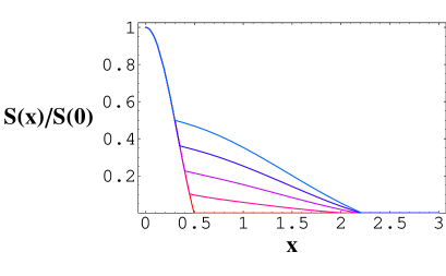
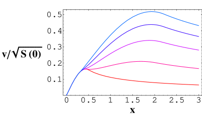
Figure 6: The behavior of the total density of scalar bosons as the function of the rescaled distance $x$, for $x_{2}=0.3,0.35,0.4,0.45,0.5$, when $C_{11}=C_{22}=1$, $C_{12}=0.9$.

Figure 7: The galaxy rotation curves induced by the bi-scalar boson stars for $x_{2}=0.3,0.35,0.4,0.45,0.5$, when $C_{11}=C_{22}=1$, $C_{12}=0.9$. Note that overall scale can be arbitrarily chosen.

In FIG. 7, we show the various profiles of the boson stars for $x_{2}=0.3,0.35,0.4,0.45,0.5$, when $C_{11}=C_{22}=1$, $C_{12}=0.9$. The rotation speed $v$ of any object in the circular motion with radius $x$ in the Newton potential $\Phi(x)$ is proportional to $\sqrt{x\Phi^{\prime}(x)}$. In the vacuum region, $\Phi(x)$ is proportional to $-M/x$, where $M$ is the total mass of the boson star. Then, the rotation velocity $v$ becomes $\propto\sqrt{M/x}$ outside the boson star. We exhibit $v/\sqrt{S(0)}=\sqrt{x\Phi^{\prime}(x)}/\sqrt{S(0)}$ for $x_{2}=0.3,0.35,0.4,0.45,0.5$ in FIG. 7. Because the potential spreads out by the density tail due to $\rho_{1}(x)$, the rotation curve can have a flat region, especially around $x_{2}\approx 0.45$ in this case. If a single scalar field model is considered, which is realized by $\rho_{2}(x)\equiv 0$, the range of the gravitational potential becomes narrow and the rotation curve looks far from a satisfactory explanation of the observational data. It is interesting to point out that if the fraction of boson 2 is much larger ($\approx 0.5$, when $x_{2}\approx\pi\omega_{2}^{-1}$), the profile of the boson star becomes much alike a single-scalar boson star. This fact can be read from the rotation curve in FIG. 7.

So far, we have picked up an example of the couplings $C_{11}=C_{22}=1$ and $C_{12}=0.9$. In this case, $\omega_{2}=6.32456$ and $\omega_{1}=1.41421$. The density profile near $\rho_{1}\approx 0$ decreases almost linearly in $\omega_{1}x$. On the other hand, the width of distribution in the core region is determined by $\omega_{2}^{-1}$. Therefore, the broad gravitational potential can be obtained if $\omega_{2}/\omega_{1}\gg 1$. In the above example, we find $\omega_{2}/\omega_{1}=4.472$.

To see this necessary condition more closely, we take another example with the couplings $C_{11}=C_{22}=1$ and $C_{12}=0$. In this case, we find $\omega_{2}=2$ and $\omega_{1}=1.41421$. The density profiles and the rotation curves for various values for $x_{2}$ ($x_{2}=0.8\sim 1.6$) are exhibited in FIG. 9 and FIG. 9, respectively. From this result, we confirm the necessity of the ‘hierarchy’ in the inverse length scales $\omega_{1}$ and $\omega_{2}$.

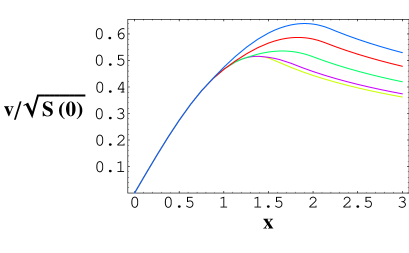
Figure 8: The behavior of the total density of scalar bosons as the function of the rescaled distance $x$, for $x_{2}=0.8,1.0,1.2,1.4,1.6$, when $C_{11}=C_{22}=1$, $C_{12}=0$.

Figure 9: The galaxy rotation curves induced by the bi-scalar boson stars for $x_{2}=0.8,1.0,1.2,1.4,1.6$, when $C_{11}=C_{22}=1$, $C_{12}=0$. Note that an overall scale can be arbitrarily chosen.

In this section, we consider the simplest bi-scalar model. We can find that the gravitational potential is spread out by the existence of $\rho_{1}$, and the tail of the boson star leads to an improvement of rotation curve of the galaxy. It is however difficult to obtain the realistic galaxy rotation curve being fit to the observational data by manipulating such a simple model. In the next and subsequent sections, we examine multi-scalar models, since the rotation curve may have the multi-scale structure.

V Spherical boson stars of multi-scalar fields with a diagonal coupling matrix

Hereafter, we consider self-interacting $[U(1)]^{N}$ scalar field theory. In this section, we examine the case that $[U(1)]^{N}$ symmetric scalar fields have only self-interactions in individual fields, and no mutual interaction to other scalar fields. Simply speaking, we consider the case with the coupling matrix expressed as a diagonal matrix in the present section, i.e., $C_{ij}=0$ if $i\not=j$.

To obtain the spherical static boson star solution, the equations we should solve are now

$$\frac{1}{x}\frac{d^{2}}{dx^{2}}(x\Phi(x))=S(x)\,,$$ (56)

$$\left(\Phi(x)+\frac{1}{2}C_{ii}\rho_{i}(x)\right){\rho}_{i}(x)=u_{i}{\rho}_{i}(x)\,,\quad i=1,\dots,N\,.$$ (57)

Thus, $\rho_{i}$ is given by

$$\rho_{i}(x)=\frac{2}{C_{ii}}\left(u_{i}-\Phi(x)\right)>0\qquad\mbox{or}\qquad\rho_{i}(x)=0\,.$$ (58)

We take $\rho_{i}\neq 0$ for $i=1,\dots,k$ and $\rho_{k+1}=\cdots=\rho_{N}=0$ $(1\leq k\leq N)$ without loss of generality. We then define

$$S_{k}(x)\equiv\sum_{i=1}^{k}\rho_{i}(x)=\sum_{i=1}^{k}\frac{2}{C_{ii}}\left(u_{i}-\Phi(x)\right)\,.$$ (59)

Operating the Laplacian on the both sides of the above equation and using the Poisson equation, we obtain

$$\frac{1}{x}\frac{d^{2}}{dx^{2}}(xS_{k}(x))=-\omega_{k}^{2}S_{k}(x)\,,\quad\omega_{k}^{2}=\sum_{i=1}^{k}\frac{2}{C_{ii}}\,.$$ (60)

We assume that $\rho_{i}(x)$ vanishes at $x=x_{i}$ and the outermost surface of the boson star is located at $x_{1}$, where $0=x_{N+1}<x_{N}<x_{N-1}<\dots<x_{2}<x_{1}$. All the normalized density $\rho_{i}$ take nonzero values in the region $0\leq x\leq x_{N}$. In the region $x_{k+1}\leq x\leq x_{k}$, $\rho_{N}=\dots=\rho_{k+1}=0$ and then $S(x)=S_{k}(x)$.

The general solutions of Eq. (60) are

$$S_{k}(x)=A_{k}\frac{\sin(\omega_{k}x+\delta_{k})}{x}\quad(x_{k+1}\leq x\leq x_{k})\,,$$ (61)

where $\delta_{k}$ and $A_{k}$ are constants. Note that $\delta_{N}=0$ because of the regularity at the origin.

The gravitational potential is then given by

$$\Phi(x)+const.=-A_{k}\frac{\sin(\omega_{k}x+\delta_{k})}{\omega_{k}^{2}x}\quad(x_{k+1}\leq x\leq x_{k})\,.$$ (62)

Because of the continuity of $S(x)$ and $\Phi^{\prime}(x)$, we find the condition

$$\left.\frac{-x\Phi^{\prime}(x)}{S(x)}\right|_{x=x_{k}}=\frac{\omega_{k}x_{k}\cot(\omega_{k}x_{k}+\delta_{k})-1}{\omega_{k}^{2}}=\frac{\omega_{k-1}x_{k}\cot(\omega_{k-1}x_{k}+\delta_{k-1})-1}{\omega_{k-1}^{2}}\,.$$ (63)

This is the recursive equation to determine the value of $\delta_{i-1}$ from $\delta_{i}$ when the other parameters are given.

First of all, we take the simplest case, $C_{ii}=1$ and $C_{ij}=0$ for $i\not=j$, i.e., the coupling matrix $\mathcal{C}=(C_{ij})$ is the identity matrix. In this case, because

$$\omega_{k}^{2}=2k\,,$$ (64)

the relation $\omega_{N}>\cdots>\omega_{1}$ holds. As we have seen in the previous section, we need a ‘hierarchy’ in $\omega$ to obtain the boson star profile with a small core and a long tail. For sufficiently large $N$, this condition is satisfied since $\omega_{N}/\omega_{1}=\sqrt{N}\gg 1$.

We show a typical case of $N=10$ in FIG. 11 and FIG. 11, where $\{x_{10},x_{9},x_{8},x_{7},x_{6},x_{5},x_{4},x_{3},x_{2}\}=\{0.43,0.48,0.53,0.58,0.63,0.68,0.73,0.78,0.83\}$. In this case, $\omega_{10}/\omega_{1}=3.16$.

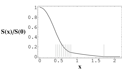
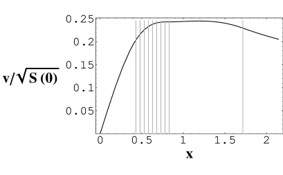
Figure 10: The behavior of the total density of ten-scalar bosons as the function of the rescaled distance $x$ when $C_{11}=\cdots=C_{10,10}=1$, $C_{ij}=0$. We take $\{x_{10},x_{9},x_{8},x_{7},x_{6},x_{5},x_{4},x_{3},x_{2}\}=\{0.43,0.48,0.53,0.58,0.63,0.68,0.73,0.78,0.83\}$ as indicated by gray vertical lines. The most right line indicates $x_{1}$, the surface of the boson star.

Figure 11: The galaxy rotation curves induced by the ten-scalar boson stars when $C_{11}=\cdots=C_{10,10}=1$, $C_{ij}=0$ for $i\neq j$. We take $\{x_{10},x_{9},x_{8},x_{7},x_{6},x_{5},x_{4},x_{3},x_{2}\}=\{0.43,0.48,0.53,0.58,0.63,0.68,0.73,0.78,0.83\}$ as indicated by gray vertical lines. The most right line indicates $x_{1}$, the surface of the boson star. Note that overall scale can be arbitrarily chosen.

For the sake of comparison, we show the case with $N=5$ in FIG. 13 and FIG. 13, where $\{x_{5},x_{4},x_{3},x_{2}\}=\{0.85,0.9,0.95,1\}$. Because $\omega_{5}/\omega_{1}$ equals $1.73$, which is not so large enough, a small core and a long tail can hardly be obtained even if we choose a smaller value for $x_{5}$, so on.

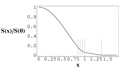
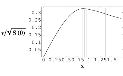
Figure 12: The behavior of the total density of five-scalar bosons as the function of the rescaled distance $x$ when $C_{11}=\cdots=C_{55}=1$, $C_{ij}=0$ for $i\neq j$. We take $\{x_{5},x_{4},x_{3},x_{2}\}=\{0.85,0.9,0.95,1\}$ as indicated by gray vertical lines. The most right line indicates $x_{1}$, the surface of the boson star.

Figure 13: The galaxy rotation curves induced by the five-scalar boson stars when $C_{11}=\cdots=C_{55}=1$, $C_{ij}=0$ for $i\neq j$. We take $\{x_{5},x_{4},x_{3},x_{2}\}=\{0.85,0.9,0.95,1\}$ as indicated by gray vertical lines. The most right line indicates $x_{1}$, the surface of the boson star. Note that overall scale can be arbitrarily chosen.

Next, we consider the case that the coupling matrix is not the identity matrix but a general diagonal matrix. As for a typical case, the profile of a five-scalar boson star and the rotation curves are shown FIG. 15 and FIG. 15, respectively. Here, we take $\mathcal{C}=diag.(5,4,3,2,1)$ and $\{x_{5},x_{4},x_{3},x_{2}\}=\{1.25,1.35,1.45,1.55\}$. Then we find that $\omega_{5}/\omega_{1}=3.38$.

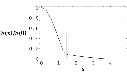
Figure 14: The behavior of the total density of five-scalar bosons as the function of the rescaled distance $x$ when $\mathcal{C}=diag.(5,4,3,2,1)$. We take $\{x_{5},x_{4},x_{3},x_{2}\}=\{1.25,1.35,1.45,1.55\}$ as indicated by gray vertical lines. The most right line indicates $x_{1}$, the surface of the boson star.

Figure 15: The galaxy rotation curves induced by the five-scalar boson stars when $\mathcal{C}=diag.(5,4,3,2,1)$. We take $\{x_{5},x_{4},x_{3},x_{2}\}=\{1.25,1.35,1.45,1.55\}$ as indicated by gray vertical lines. The most right line indicates $x_{1}$, the surface of the boson star. Note that overall scale can be arbitrarily chosen.

In this section, the large number of scalar fields and/or the large hierarchy in the couplings is necessary for a flat rotation curve, in the case of the diagonal coupling matrix. Both the large number of the fields and the hierarchy in couplings ruin the simpleness of the original theory, which is implicitly desired in theoretical models.

In the next section, we investigate more general coupling matrix including mutual interactions among scalar fields. Since we prefer the model with some symmetry, we propose models associated with a certain symmetric ‘graph’, which appears in graph theory, in the next section.

VI a mutually-coupled scalar model associated with a graph Laplacian

We start with a general case with non-diagonal coupling matrix $\mathcal{C}=(C_{ij})$. We assume that $\rho_{i}>0$ for $i=1,\dots,k$ and $\rho_{k+1}=\dots=\rho_{N}=0$ in the region $x_{k+1}<x<x_{k}$. Then the algebraic equation for nonzero $\rho_{i}(x)$ can be expressed as

$$\Phi(x)\mathbf{w}_{[k]}+\frac{1}{2}\mathcal{C}_{[k]}\mathbf{\rho}_{[k]}(x)=\mathbf{u}_{[k]}\,,$$ (65)

where $\mathcal{C}_{[k]}$ is a $k\times k$ principal submatrix of the matrix $\mathcal{C}$ defined as

$$\mathcal{C}_{[k]}\equiv\left(\begin{array}[]{rrrr}C_{11}&C_{12}&\cdots&C_{1k}\\ C_{21}&C_{22}&\cdots&C_{2k}\\ \vdots&\vdots&\ddots&\vdots\\ C_{k1}&C_{k2}&\cdots&C_{kk}\end{array}\right)\,,$$ (66)

whereas $\mathbf{w}_{[k]}$, $\mathbf{\rho}_{[k]}(x)$ and $\mathbf{u}_{[k]}$ are vectors with $k$ components given by

$$\mathbf{w}_{[k]}\equiv(1,1,\dots,1)^{\rm T}\,,\quad\mathbf{\rho}_{[k]}(x)\equiv(\rho_{1}(x),\rho_{2}(x),\dots,\rho_{k}(x))^{\rm T}\,,\quad\mathbf{u}_{[k]}\equiv(u_{1},u_{2},\dots,u_{k})^{\rm T}\,.$$ (67)

Note that $\mathcal{C}_{[N]}=\mathcal{C}$.

In the region $x_{k+1}<x<x_{k}$, $\mathbf{\rho}_{[k]}(x)$ can be solved as

$$\mathbf{\rho}_{[k]}=-2\mathcal{C}_{[k]}^{-1}(\Phi\mathbf{w}_{[k]}-\mathbf{u}_{[k]})\,,$$ (68)

where $\mathcal{C}_{[k]}^{-1}$ is the inverse of $\mathcal{C}_{[k]}$. Then, we find

$$S_{k}(x)=\sum_{i=1}^{k}\rho_{i}(x)=-2\mathbf{w}_{[k]}^{\rm T}\mathcal{C}_{[k]}^{-1}(\Phi(x)\mathbf{w}_{[k]}-\mathbf{u}_{[k]})\,.$$ (69)

As in the previous sections, by using the gravitational Poisson equation, we obtain

$$\frac{1}{x}\frac{d^{2}}{dx^{2}}(xS_{k}(x))=-\omega_{k}^{2}S_{k}(x)\quad(x_{k+1}<x<x_{k})\,,$$ (70)

where

$$\omega_{k}^{2}=2\mathbf{w}_{[k]}^{\rm T}\mathcal{C}_{[k]}^{-1}\mathbf{w}_{[k]}\,.$$ (71)

Now, since we obtain $\omega_{k}^{2}$, we can evaluate the profile of the boson star and the gravitational potential by the same method as in the previous sections.

In the rest of this section, we consider a concrete model whose coupling matrix is represented by a graph Laplacian, which appears in texts of spectral graph theory mohar1 ; mohar2 ; mohar3 ; merris ; GR ; CRS .

Let $G(\mathcal{V},\mathcal{E})$ be a graph with a vertex set $\mathcal{V}$ and an edge set $\mathcal{E}$. The set of edges connects the vertices. A pair of vertices $v$ and $v^{\prime}$ are said to be adjacent, denoted $v\sim v^{\prime}$, if there exists an edge which connects $v$ and $v^{\prime}$. The degree of a vertex $v$, denoted $deg(v)$, is the number of edges directly connected to $v$.

The graph Laplacian $\triangle(G)$ of the graph $G$ is defined by

$$(\triangle(G))_{vv^{\prime}}=\left\{\begin{array}[]{cl}deg(v)&\mbox{if }~{}v=v^{\prime}\\ -1&\mbox{if }~{}v\sim v^{\prime}\\ 0&\mbox{otherwise}\end{array}\right.\,,$$ (72)

where $v,v^{\prime}\in\mathcal{V}$.

Now, we take a model whose coupling matrix can be written as

$$\mathcal{C}=\mathcal{I}+\gamma\triangle(G)\,,$$ (73)

where $\mathcal{I}$ is the $N\times N$ identity matrix and $\gamma$ is a non-negative constant. Here, we suppose that the graph $G$ has $N$ vertices. We inversely find the scalar quartic interaction in this model has the form

$$V(|\phi_{i}|^{2})\propto\sum_{v\in{\cal V}}|\phi_{v}|^{4}+\gamma\sum_{v\sim v^{\prime}}(|\phi_{v}|^{2}-|\phi_{v^{\prime}}|^{2})^{2}\,,$$ (74)

where the second sum is done once over all adjacent pairs, and then we find the potential is obviously positive-semidefinite. The use of the graph Laplacian guarantees the positivity of the potential energy in the model.

Figure 16: A complete graph $K_{5}$.

First of all, we adopt a complete graph $K_{N}$ as a maximally symmetric graph. In a complete graph, each vertex is adjacent to all the other vertices (FIG. 16). The model based on a complete graph is most democratic, because the potential is invariant under any exchange of scalar field species, in other words, vertices in a complete graph have a symmetry under the symmetric group $S_{N}$. The graph Laplacian of the complete graph with $N$ vertices is

$$\triangle(K_{N})=\left(\begin{array}[]{ccccc}N-1&-1&-1&\cdots&-1\\ -1&N-1&-1&\cdots&-1\\ -1&-1&N-1&\cdots&-1\\ \vdots&\vdots&\vdots&\ddots&\vdots\\ -1&-1&-1&\cdots&N-1\end{array}\right)\,.$$ (75)

To obtain $\omega_{k}^{2}$, we have to calculate the matrix $\mathcal{C}_{[k]}^{-1}$. We consider the eigenvectors of the matrix $\mathcal{C}_{[k]}$, which is denoted by $\mathbf{v}_{[k]}^{a}$ $(a=0,\dots,k-1)$. They satisfy

$$\mathcal{C}_{[k]}\mathbf{v}_{[k]}^{a}=\lambda_{[k]}^{a}\mathbf{v}_{[k]}^{a}\,,\quad(\mathbf{v}_{[k]}^{a})^{\rm T}\mathbf{v}_{[k]}^{b}=\delta^{ab}\,,$$ (76)

where $\lambda_{[k]}^{a}$ is the eigenvalues of the matrix $\mathcal{C}_{[k]}$. Then, we can express the inverse matrix using the eigenvalues and the eigenvectors of the matrix as

$$\mathcal{C}_{[k]}^{-1}=\sum_{a}\mathbf{v}_{[k]}^{a}\frac{1}{\lambda_{[k]}^{a}}(\mathbf{v}_{[k]}^{a})^{\rm T}\,.$$ (77)

In the present case that $\mathcal{C}=\mathcal{I}+\gamma\triangle(K_{N})$, the vector $\frac{1}{\sqrt{k}}\mathbf{w}_{[k]}$ is an eigenvector of $\mathcal{C}_{[k]}$ for any $k$, and the associated eigenvalue is $1+\gamma(N-k)$. Therefore,

$$\omega_{k}^{2}=2\mathbf{w}_{[k]}^{\rm T}\mathcal{C}_{[k]}^{-1}\mathbf{w}_{[k]}=2\mathbf{w}_{[k]}^{\rm T}\mathbf{w}_{[k]}\frac{1}{k[1+\gamma(N-k)]}\mathbf{w}_{[k]}^{\rm T}\mathbf{w}_{[k]}=\frac{2k}{1+\gamma(N-k)}\,,$$ (78)

where we used the orthogonal relation among the eigenvectors.

The necessary condition for a ‘small core and long tail’ boson star solution is that the ratio $\omega_{N}/\omega_{1}$ is much larger than unity, actually $\omega_{N}/\omega_{1}\stackrel{{\scriptstyle>}}{{\sim}}3\sim 4$. In the present model, we find

$$\frac{\omega_{N}}{\omega_{1}}=\sqrt{N(1+\gamma(N-1))}\sim\gamma^{1/2}N\,,$$ (79)

so, the choice of $\gamma\simeq 1$ and $N\simeq 3\sim 4$ satisfies the condition.

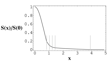
Figure 17: The behavior of the total density of five-scalar bosons as the function of the rescaled distance $x$ in the model associated with a complete graph $K_{5}$ and $\gamma=1$. We take $\{x_{5},x_{4},x_{3},x_{2}\}=\{0.83,1.03,1.23,1.43\}$ as indicated by gray vertical lines. The most right line indicates $x_{1}$, the surface of the boson star.

Figure 18: The galaxy rotation curves induced by the five-scalar boson stars in the model associated with a complete graph $K_{5}$ and $\gamma=1$. We take $\{x_{5},x_{4},x_{3},x_{2}\}=\{0.83,1.03,1.23,1.43\}$ as indicated by gray vertical lines. The most right line indicates $x_{1}$, the surface of the boson star. Note that overall scale can be arbitrarily chosen.

We demonstrate the calculation for $N=5$, $\gamma=1$, and $\{x_{5},x_{4},x_{3},x_{2}\}=\{0.83,1.03,1.23,1.43\}$, and show the results in FIG. 18 and FIG. 18. By integrating densities, we can evaluate the particle number of each scalar boson. The fraction of species are $\{n_{1}/n,n_{2}/n,n_{3}/n,n_{4}/n,n_{5}/n\}=\{0.786,0.0788,0.0620,0.0453,0.0283\}$, where $n=\sum_{i=1}^{5}n_{i}$. Although the value of $n_{1}/n$ is larger than those of others, because of the long tail distribution of the boson star, this composition is not so unnatural. The contribution of each boson species are shown in FIG. 19.

Figure 19: The contribution of each boson species in the model associated with $K_{5}$ and $\gamma=1$. We take $\{x_{5},x_{4},x_{3},x_{2}\}=\{0.83,1.03,1.23,1.43\}$. The curves indicate $S_{k}(x)=\sum_{i=1}^{k}\rho_{i}(x)$, $k=5$ to $1$, from the upper to the lower.

Thus, we have found that the model with the coupling matrix associated with the graph Laplacian of the complete graph leads to flat rotation curves in a natural setting, for comparatively small number of scalar fields which have symmetry under any exchange of species. Moreover, a small but finite number of fields brings about a diversity of galaxy rotation curves, as observations indicate. It can be recognized that the variation on diverse galaxies is due to the set of fractions of the particle numbers.

Figure 20: A cycle graph $C_{10}$.

Figure 21: A star graph with five vertices.

Next, we consider the use of the other graphs in the coupling matrix. We now consider a cycle graph $C_{N}$ (FIG. 21). The coupling matrix is given in the same form Eq. (73), as previously considered. The model based on a cycle graph still has discrete symmetry under $\phi_{i}\rightarrow\phi_{i+l}~{}(\mbox{mod }N)$, where $l$ is an integer.

The graph Laplacian of a cycle graph $C_{N}$ takes the form

$$\triangle(C_{N})=\left(\begin{array}[]{cccccc}2&-1&0&\cdots&0&-1\\ -1&2&-1&\cdots&0&0\\ 0&-1&2&\cdots&0&0\\ \vdots&\vdots&\vdots&\ddots&\vdots&\vdots\\ 0&0&0&\cdots&2&-1\\ -1&0&0&\cdots&-1&2\end{array}\right)\,.$$ (86)

In the model associated with $\triangle(C_{N})$, we find

$$\omega_{N}^{2}=2\mathbf{w}_{[N]}^{\rm T}\mathcal{C}^{-1}\mathbf{w}_{[N]}=2N\quad\mbox{and}\quad\omega_{1}^{2}=2{C}_{11}^{-1}=\frac{2}{1+2\gamma}\,.$$ (87)

Note that $\frac{1}{\sqrt{N}}\mathbf{w}_{[N]}$ is the eigenvector belonging to zero eigenvalue for any simple graph Laplacian. Therefore, we find

$$\frac{\omega_{N}}{\omega_{1}}=\sqrt{N(1+2\gamma)}\sim\sqrt{N}\,.$$ (88)

In general, the necessary condition in this model is more severe than that in the model associated with a complete graph, but a sufficiently large number of scalar fields satisfies the condition. In a loosely connected graph such as a cycle graph, each degree of the vertex is much smaller than $N-1$. Thus, $\omega_{1}$ tends to be larger than the case with a complete graph. In the star graph with $N$ vertices (FIG. 21), the maximal degree of the vertex is $N-1$, which is the same as that in a complete graph. Then, in the model based on the star graph, the ratio ${\omega_{N}}/{\omega_{1}}$ takes the same value as that in the model of the complete graph $K_{N}$ with the same number $N$ of scalar species. However, the model associated with the star graph with $N$ vertices has less symmetry, i.e. symmetric under the symmetric group $S_{N-1}$ rather than $S_{N}$.

Recently, models with mass hirarchy generated by the ‘clockwork mechanism’ CI ; KaRa ; GM1 ; FPRT ; KeRi ; HTT ; teresi ; AD ; CGS ; GM2 are eagerly investigated by many authors. If it is feasible to use the same structure in our coupling matrix instead of their mass matrices, we would have an interesting model for boson stars constructed by several fields.

VII Summary and outlook

In the present paper, we have examined the Newtonian boson star with many $U(1)$ charges in the large coupling limit. The explanation of rotation curves of galaxies by gigantic boson stars is improved in this model.

The necessary condition for a flat rotation curve is that $\omega_{N}$ is several times larger than $\omega_{1}$ in terms of our model parameter. This is naturally led from the model with a large number of scalar field and/or the model whose coupling matrix is associated with the graph Laplacian of the complete graph. The latter model has larger symmetry on several scalar fields. It is worth pointing out that several species of bosons are necessary to make a variety in the rotation curves of different galaxies, even including dwarf galaxies.

In the present paper, we have concentrated ourselves on the galactic boson stars. The structure of small multi-scalar boson stars is still similar because of the scale invariance of our models. It will be interesting to find some new aspects of the boson stars in various circumstances, such as in a collision of multi-scalar boson stars.

Although the model we have demonstrated is rather a toy model and has only been focused as in the large coupling limit, it is the simplest effective theory of multi-scalar boson stars. As a variant of the model, it is interesting to consider the case that there exist other fields which do not participate the ingredient of the boson star but affect on the creation or decay of boson stars. Anyway, we would like to find the relevance of the multi-scalar theory to particle physics, and wish to clarify its role or significance.

In future work, we will consider general relativistic boson stars and graph-oriented models with many charges or arbitrary couplings. We also have much interest on boson stars in plausible models in which finite or zero couplings. It is known that single-scalar boson stars with finite self-couplings can also be approximated analytically by connecting the exponential tail in the asymptotic region of the boson star GA . Since the rotation curve is most sensitive on the tail of the boson star, analyses of models with finite self-couplings should be performed as in the next step. Time dependent solutions or oscillations of multiple scalar fields are also interesting. We wish to investigate these subjects elsewhere.

Appendix A a multi-scalar boson star with an external gravitational source

The realistic galaxies have bulges and halos of stars and gas, which are gravitational sources and are expected not to interact with scalar fields in our model (and other unknown dark stuff).

In the presence of the nonnegligible external gravitational source, whose energy density is given by $\rho_{ext}$ other than the scalar fields, we add an inhomogenious term in the right hand side of Eq. (56) as

$$\frac{1}{x}\frac{d^{2}}{dx^{2}}(x\Phi(x))=S(x)+\bar{\rho}_{ext}(x)\,,$$ (89)

where $\bar{\rho}_{ext}=4\pi G\Lambda/m^{2}\rho_{ext}$. Although the normalization seems to be strange, the ratio of energy densities are nevertheless simply given by $\bar{\rho}_{ext}/S$. Now, we should solve the differential equations

$$\frac{1}{x}\frac{d^{2}}{dx^{2}}(xS_{k}(x))+\omega_{k}^{2}S_{k}(x)=-\omega_{k}^{2}\bar{\rho}_{ext}(x)\quad(x_{k+1}<x<x_{k})\,,$$ (90)

and the special solution for the inhomogeneous term is found to be

$$-\frac{\omega_{k}}{x}\int_{x_{k+1}}^{x}t\bar{\rho}_{ext}(t)\sin\omega_{k}(x-t)dt\quad(x_{k+1}<x<x_{k})\,.$$ (91)

Since a main subject of the present paper is an interest in analytical study, we consider a simple example in this appendix. We now assume

$$\bar{\rho}_{ext}(x)=A_{e}\frac{\sin\omega_{e}x}{x}\quad(0<x<\pi/\omega_{e})\,,$$ (92)

where $A_{e}$ and $\omega_{e}$ are constants and $\bar{\rho}_{ext}(x)=0$ for $x>\pi/\omega_{e}\equiv x_{N+1}$. We further assume $\omega_{e}>\omega_{N}$ for simplicity. Then, we find

$$S_{N+1}(x)=A_{N}\frac{\sin\omega_{N}x}{x}+\frac{A_{e}}{\omega_{e}^{2}/\omega_{N}^{2}-1}\frac{\sin\omega_{e}x}{x}\quad(0<x<\pi/\omega_{e}=x_{N+1})\,,$$ (93)

where $A_{N}$ is an arbitrary constant. We have only to find the total solutions by the connection condition of $-x\Phi^{\prime}/S$ as in Sec. V.

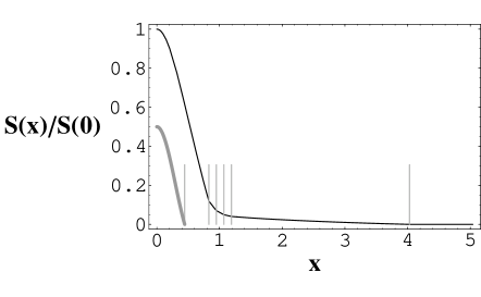
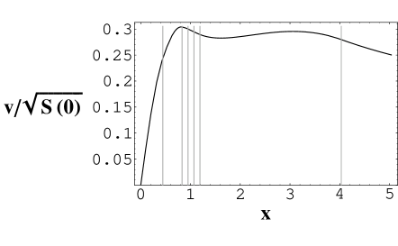
Figure 22: The behavior of the total density of five-scalar bosons as the function of the rescaled distance $x$ in the model associated with a complete graph $K_{5}$ and $\gamma=1$, in the presence of the external gravitational source (see text) with $\omega_{e}=\sqrt{5}\omega_{5}$ and $\bar{\rho}_{ext}(0)/S(0)=0.5$. The gray curve in the figure shows $\bar{\rho}_{ext}(x)$. We take $\{x_{6},x_{5},x_{4},x_{3},x_{2}\}=\{0.44,0.83,0.95,1.07,1.19,1.31\}$ as indicated by gray vertical lines. The most right line indicates $x_{1}$, the surface of the boson star.

Figure 23: The galaxy rotation curves induced by the five-scalar boson stars in the model associated with a complete graph $K_{5}$ and $\gamma=1$, in the presence of the external gravitational source (see text) with $\omega_{e}=\sqrt{5}\omega_{5}$ and $\bar{\rho}_{ext}(0)/S(0)=0.5$. We take $\{x_{5},x_{4},x_{3},x_{2}\}=\{0.44,0.83,0.95,1.07,1.19,1.31\}$ as indicated by gray vertical lines. The most right line indicates $x_{1}$, the surface of the boson star. Note that overall scale can be arbitrarily chosen.

A result in the model associated with $K_{5}$ in Sec. VI is shown in FIG. 23 and FIG. 23, where we set $\omega_{e}=\sqrt{5}\omega_{5}$, $\bar{\rho}_{ext}(0)/S(0)=0.5$ and $\{x_{5},x_{4},x_{3},x_{2}\}=\{0.44,0.83,0.95,1.07,1.19,1.31\}$. The most appropriate parameter set for a flat rotation curve, of course, changes slightly by the effect of the gravitational source. Conversely, it would be said that the density profle from the present model can be adjusted to various distributions of ordinary matter in many galaxies.

References

(1) P. Jetzer,
Phys. Rep. 220 (1992) 163.
(2) A. R. Liddle and M. S. Madsen,
Int. J. Mod. Phys. D1 (1992) 101.
(3) F. E. Schunck and E. W. Mielke,
Class. Quant. Grav. 20 (2003) R301.
(4) S. L. Liebling and C. Palenzuela,
Living Rev. Relativity 15 (2012) 6.
(5) F. E. Schunck and A. R. Liddle,
Phys. Lett. B404 (1997) 25.
(6) F. E. Schunck and A. R. Liddle,
“Boson stars in the centre of galaxies?” in
“Black Holes: Theory and Observation”,
Proceedings of the Bad Honnef Workshop,
F. W. Hehl, C. Kiefer and R. J. K. Metzler eds. (Springer-Verlag, Berlin,
1998), pp. 285–288, arXiv:0811.3764 [astro-ph].
(7) J. W. Lee and I. G. Koh,
Phys. Rev. D53 (1996) 2236.
(8) D. F. Torres, S. Capozziello and G. Lambiase,
Phys. Rev. D62 (2000) 104012.
(9) F. E. Schunck and D. F. Torres,
Int. J. Mod. Phys. D9 (2000) 601.
(10)
P. Amaro-Seoane, J. Barranco, A. Bernal and L. Rezzolla,
JCAP 1011 (2010) 002.
(11)
T. Matos and L. A. Ureña-López,
Gen. Rel. Grav. 39 (2007) 1279.
(12) A. Bernal, J. Barranco, D. Alic and C. Palenzuela,
Phys. Rev. D81 (2010) 044031.
(13)
R. Ferrell and M. Gleiser,
Phys. Rev. D40 (1989) 2524.
(14)
S.-J. Sin,
Phys. Rev. D50 (1994) 3650.
(15)
S. U. Ji and S.-J. Sin,
Phys. Rev. D50 (1994) 3655.
(16)
N. Kan and K. Shiraishi,
Phys. Rev. D94 (2016) 104042.
(17)
F. E. Schunck,
arXiv:astro-ph/9802258.
(18)
Y. Brihaye, T. Caebergs, B. Hartmann and M. Minkov,
Phys. Rev. D80 (2009) 064014.
(19)
Y. Brihaye and B. Hartmann,
Phys. Rev. D79 (2009) 064013.
(20)
Y. Brihaye and B. Hartmann,
Nonlinearity 21 (2008) 1937.
(21)
N. Kan, K. Kobayashi and K. Shiraishi,
Phys. Rev. D80 (2009) 045005.
(22) M. Colpi, S. L. Shapiro and I. Wasserman,
Phys. Rev. Lett. 57 (1986) 2485.
(23)
B. Mohar, “The Laplacian spectrum of graphs” in “Graph Theory,
Combinatorics, and Applications”, Y. Alavi et al. eds. (Wiley, New York,
1991), pp. 871–898.
(24)
B. Mohar,
Discrete Math. 109 (1992) 171.
(25)
B. Mohar, “Some Applications of Laplace Eigenvalues of
Graphs” in “Graph Symmetry, Algebraic Methods, and Applications”, G. Hahn
and G. Sabidussi eds. (Kluwer, Dordrecht, 1997), pp. 225–275.
(26)
R. Merris,
Linear Algebra Appl. 197 (1994) 143.
(27)
C. Godsil and G. Royle, “Algebraic Graph Theory” (New York: Springer,
2001).
(28)
D. Cvetković, P. Rowlinson and S. Simić, “An Introduction to the Theory
of Graph Spectra” (London Mathematical Society Student Texts 75) (Cambridge:
Cambridge University Press, 2010).
(29)
K. Choi and S. H. Im,
JHEP 1601 (2016) 149.
(30)
D. E. Kaplan and R. Rattazzi,
Phys. Rev. D93 (2016) 085007.
(31)
G. F.Giudice and M. McCullough,
JHEP 1702 (2017) 036.
(32)
M. Farina, D. Pappadopulo, F. Rompineve and A. Tesi,
JHEP 1701 (2017) 095.
(33)
A. Kehagias and A. Riotto,
Phys. Lett. B767 (2017) 73.
(34)
T. Hambye, D. Teresi and M. H. G. Tytgat,
JHEP 1707 (2017) 47.
(35)
D. Teresi,
arXiv:1705.09698 [hep-ph].
(36)
A. Ahmed and B. M. Dillon,
arXiv:1612.04011 [hep-ph].
(37)
N. Craig, I. Garcia Garcia and D. Sutherland,
arXiv:1704.07831 [hep-ph].
(38)
G. F. Giudice and M. McCullough,
arXiv:1705.10162 [hep-ph].
(39)
A. Bernal and F. S. Guzmán,
Phys. Rev. D74 (2006) 103002.
(40)
J. A. González and F. S. Guzmán,
Phys. Rev. D83 (2011) 103513.
(41)
F. S. Guzmán and L. A. Ureña-López,
Phys. Rev. D68 (2003) 024023.