OGLE-2016-BLG-0168 Binary Microlensing Event: Prediction and Confirmation of the Micorlens Parallax Effect from Space-based Observation

Abstract

The microlens parallax is a crucial observable for conclusively identifying the nature of lens systems in microlensing events containing or composed of faint (even dark) astronomical objects such as planets, neutron stars, brown dwarfs, and black holes. With the commencement of a new era of microlensing in collaboration with space-based observations, the microlens parallax can be routinely measured. In addition, space-based observations can provide opportunities to verify the microlens parallax measured from ground-only observations and to find a unique solution of the lensing lightcurve analysis. However, since most space-based observations cannot cover the full lightcurves of lensing events, it is also necessary to verify the reliability of the information extracted from fragmentary space-based lightcurves. We conduct a test based on the microlensing event OGLE-2016-BLG-0168 created by a binary lens system consisting of almost equal mass M-dwarf stars to demonstrate that it is possible to verify the microlens parallax and to resolve degeneracies by using the space-based lightcurve even though the observations are fragmentary. Since space-based observatories will frequently produce fragmentary lightcurves due to their short observing windows, the methodology of this test will be useful for next-generation microlensing experiments that combine space-based and ground-based collaboration.

1. Introduction

The microlensing technique can probe a variety of astronomical objects in a wide range of masses such as planets, neutron stars, brown dwarfs, and isolated black holes (Dong et al., 2007; Miyake et al., 2012; Poindexter et al., 2005; Shvartzvald et al., 2015; Wyrzykowski et al., 2016). The microlensing technique can detect these faint or dark objects regardless of their luminosity levels, in sharp contrast to other methods, which as a matter of course are restricted to studying objects within their flux detection limits.

To conclusively reveal the nature of the lens system that generates a microlensing event, additional observables are required such as the microlens parallax, $\pi_{\rm E}$, and the angular Einstein ring radius, $\theta_{\rm E}$. Based on these additional observables, the properties of the lens system can be determined from

$$M_{\rm L}={\theta_{\rm E}\over\kappa\pi_{\rm E}}~{}~{};~{}~{}D_{\rm L}={{\rm AU}\over{\pi_{\rm E}\theta_{\rm E}+\pi_{\rm S}}},$$ (1)

where $M_{\rm L}$ is the total mass of the lens system, $D_{\rm L}$ is the distance to the lens system toward the Galactic bulge, $\pi_{\rm S}$ is the parallax of the background star (source) defined as $\pi_{\rm S}={\rm AU}/D_{\rm S}$ where the $D_{\rm S}$ is the distance to the source, and $\kappa\equiv 4G/(c^{2}{\rm AU})\sim 8.1~{}{\rm mas}/M_{\odot}$. Although $\pi_{\rm E}$ and $\theta_{\rm E}$ appear equally important in Equation (1), $\pi_{\rm E}$ is actually more crucial because $\theta_{\rm E}$ is easily determined from the finite source effect with high-cadence observations. In particular, for a binary lensing event, $\theta_{\rm E}$ can be routinely measured when the source crosses or approaches caustics of binary lensing events. Thus, it is important to securely and accurately measure the microlens parallax.

However, the measurement of the microlens parallax based on ground-only observations is made from subtle deviations in those lensing lightcurves that have a sufficiently long time-scale to make manifest the deviations caused by Earth’s orbital motion. As a result, there exist some obstacles to measuring the microlens parallax. First, the signal of the microlens parallax, i.e., subtle deviations in the lightcurve, can be detected if Earth moves enough to produce the signal over the duration of the event. Thus, the microlens parallax can be measured for only some cases of lensing events that have long time-scales (usually, $t_{\rm E}\geq 30$ days). Second, the measurement can be confused with systematics that can make a false positive detection or inaccurate measurement of the microlens parallax. Third, there exist degeneracies in the microlens parallax that prevent accurately or uniquely measuring it. For example, the ecliptic degeneracy (Jiang et al., 2004; Skowron et al., 2011) produces degenerate solutions with different values of the microlens parallax that can describe the same lensing lightcurve. Also, the lens-orbital effect caused by orbital motion of the lens components affects the measured values of the microlens parallax (Batista et al., 2011; Shin et al., 2012; Skowron et al., 2011). Hence, before the era of space-based microlensing, the microlens parallax could be securely and accurately measured for only a small number of lensing events that satisfy conditions to measure it during a bulge season.

In the new era, however, the microlens parallax can be routinely and securely measured in collaboration with space-based observations. In principle, the offset between ground and space telescopes provides a chance to routinely measure the microlens parallax regardless of the magnification level of the lensing event. In addition, space-based observations can provide opportunities to verify the measurement of the microlens parallax and to resolve degeneracies in the microlens parallax.

However, for lensing events having a relatively long time-scale, space-based observations can cover only fragmentary parts of the full lensing lightcurve due to short observing windows. For example, the Spitzer space telescope has only a $\sim 40$ day observing window. Moreover, space-based observations generally do not cover caustic-crossing features of the binary lensing event because it is almost impossible to predict the exact time when the source crosses the caustic structure, especially for long-time scale events. Indeed, for single lensing events, Yee et al. (2015b) posit and Calchi Novati et al. (2015a) and Zhu et al. (2017) show that fragmentary lightcurves can be successfully exploited to extract microlens parallaxes for point-lens (or near point-lens) events. However, this has not been demonstrated for binary lensing events.

Because these fragmentary space-based lensing lightcurves are quite common, it is important to do a test whether it is possible to extract reliable information from them or not. In fact, during the Spitzer microlensing campaign in $2015-2016$, most of the observed lightcurves are fragmentary. Thus, we conduct such a test by using the binary microlensing event OGLE-2016-BLG-0168 which has Spitzer observations. The event has a long time-scale ($t_{\rm E}\sim 90$ days) and the Spitzer observations covered a short part ($\sim 30$ days) of the full lensing lightcurve. Moreover, we found degenerate solutions to the event during the analysis. As a result, this event is a perfect test bed to show the possibility of extracting information from the fragmentary lightcurve observed by a space-based observatory. Our test can provide an important example to probe the reliability of extracting information from the fragmentary space-based observations. In addition, the methodology of this test can provide procedures to systematically measure and verify the microlens parallax based on fragmentary lightcurves from space and to resolve the degenerate solutions, especially for the Spitzer microlensing campaign.

In this paper, we describe observations of the event in Section 2. In Section 3, we describe our analysis procedures and the test. In Section 4, we present results of the analysis and the test of the event. Lastly, we discuss and summarize the results in Section 5.

2. Observations

The microlensing event OGLE-2016-BLG-0168 occurred on the source star located in the galactic bulge at $(\alpha,\delta)_{\rm J2000}=(17^{h}50^{m}49^{s}.89,-31^{\circ}45^{{}^{\prime}}30^{{}^{\prime\prime}}.1)$ in equatorial coordinates and $(l,b)=(-1.84,-2.42)$ in galactic coordinates. The event was observed both by ground-based surveys and the Spitzer space telescope. In Figure 1, we present the observed lightcurve of OGLE-2016-BLG-0168. The upper two panels show the caustic-crossing parts of the lightcurve and the lower panels show the entire duration of significant magnification. The lightcurve observed from ground-based telescopes shows typical features caused by a binary lens system.

2.1. Ground-based observations

The event was announced by the Optical Gravitational Lensing Experiment (OGLE: Udalski et al., 2015a) based on observations with its 1.3 m Warsaw telescope with $1.4~{}{\rm deg^{2}}$ camera located at the Las Campanas Observatory in Chile. The event was alerted by the Early Warning System (EWS: Udalski et al., 1994; Udalski, 2003) of the OGLE survey on 2016 February 21. The OGLE data in I-band were reduced by a pipeline based on the Difference-Imaging Analysis method (Alard & Lupton, 1998; Wozniak, 2000). The uncertainties of the OGLE data were re-scaled according to the description in Skowron et al. (2016).

The Korea Microlensing Telescope Network (KMTNet: Kim et al., 2016) survey, which is designed for high-cadence monitoring toward the galactic bulge with large a field-of-view, independently observed the event. KMTNet is a telescope network consisting of three identical 1.6 m telescopes with $4~{}{\rm deg^{2}}$ cameras located at Cerro Tololo Inter-American Observatory in Chile (KMTC), South African Astronomical Observatory in South Africa (KMTS), and Siding Spring Observatory in Australia (KMTA). For the event, KMTC and KMTA observations cover the caustic entrance (${\rm HJD-2450000=HJD^{\prime}}\sim 7474.2$) and exit (${\rm HJD^{\prime}}\sim 7532.5$) parts of the lightcurve with $\sim 15$ minute cadence. KMTNet data in I-band were reduced by pySIS (Albrow et al., 2009), which employs the image subtraction method.

The event was also observed in both I- and H-band by the SMARTS 1.3 m telescope at CTIO in Chile. These data were not used in the modeling, but were used to determine the $({\it I-H})$ source color (see Section 4.4).

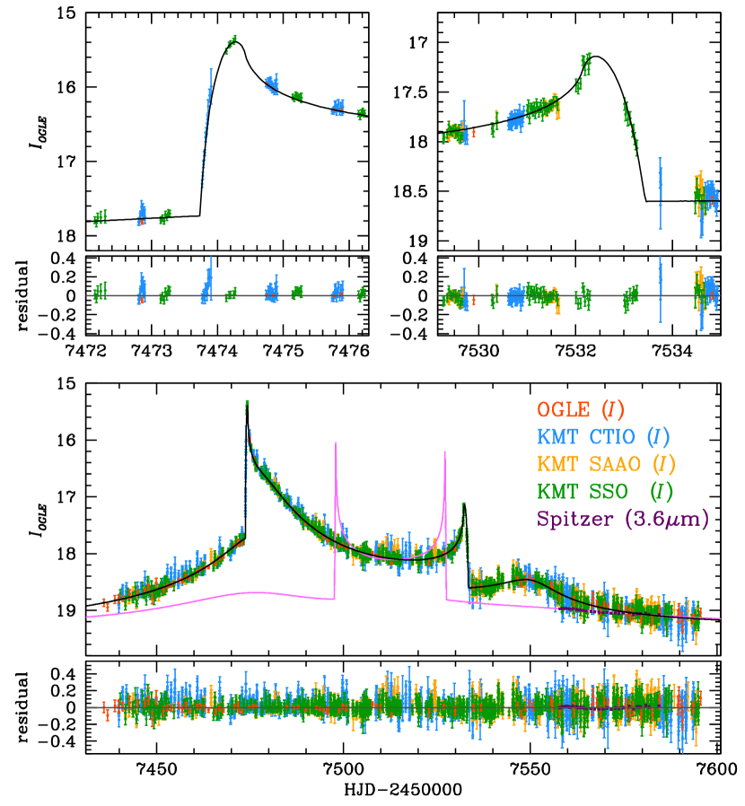
Figure 1.— Lightcurves of the binary microlensing event OGLE-2016-BLG-0168. Each color represents observed data from different telescopes located in ground and space. Black and pink solid lines indicate the model lightcurves of ground and Spitzer observations, respectively. Upper panels show the zoom-ins of the ground lightcurve the caustic entrance (left) and exit (right). Lower panels show the whole lightcurves with residuals between models and observations.

2.2. Space-based observations

The event was observed by the Spitzer space telescope with the $3.6~{}\mu m$ channel (hereafter, L-band) of the IRAC camera. Briefly, the event was selected on 2016 June 16 as a subjective target based on the selection criteria described in Yee et al. (2015b) because the lightcurve from ground-based observations showed typical anomaly features caused by the binary lens system. The observations started on 2016 June 18 (${\rm HJD^{\prime}}\sim 7557.93$) and ended July 14 (${\rm HJD^{\prime}}\sim 7584.48$). During $4$ weeks of observations with cadence $\sim 1~{}{\rm day^{-1}}$, $28$ data points of the event were gathered and then the data were reduced by using methods described in Calchi Novati et al. (2015b).

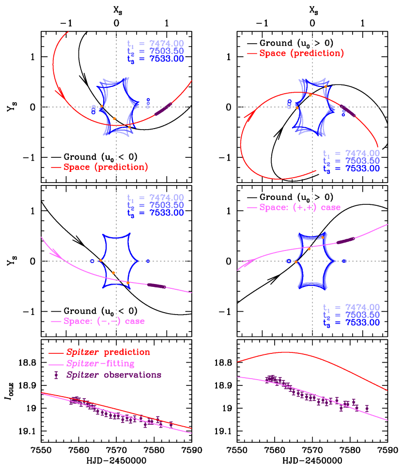
Figure 2.— Geometries of the binary microlensing event OGLE-2016-BLG-0168. Top panels show caustic features reflecting the orbital motion of the binary lens system at the time when the source enters $({\rm HJD^{\prime}}\sim 7474.0)$, is inside $(\sim 7503.5)$, and exits $(\sim 7533.0)$ the caustic; the orange dots mark the source position at those times. In the panels, the black line with an arrow indicates the source trajectory of ground-based models and the red line indicates the predicted source trajectory of the Spitzer lightcurve based on the ground models of $(u_{0}<0)$ (left) and $(u_{0}>0)$ (right) cases. The purple points represent the coverage of Spitzer observations. Middle panels show geometries of models with combined data from ground and Spitzer. The color scheme is the same as the top panel except that now a pink line indicates the Spitzer-fitted lightcurve. Bottom panels show the prediction, Spitzer-fitting, and observations of Spitzer lightcurve for both $(-,-)$ (left) and $(+,+)$ (right) cases, respectively.

2.3. Extinction

The source star of the event is located in a severely extincted field. The source extinction is $A_{I}\sim 4.9$ in I-band and $A_{L}\sim 0.35$ in L-band . As a result, the source is relatively faint for ground-based observations from OGLE and KMTNet. In contrast to ground-based observations, the source is a quite bright target for Spitzer observations.

3. Analysis

We model the lightcurves of the OGLE-2016-BLG-0168 event to reveal the nature of the binary lens system causing the microlensing event. In addition, we conduct a test to validate the microlens parallax and resolve the degeneracy in the microlens parallax.

Table 1The best-fit models of the ground-based observations

		$(u_{0}<0)$		$(u_{0}>0)$
parameter	STD	PRX	OBT+PRX	PRX	OBT+PRX
$\chi^{2}/{\rm dof}$	6501.53 / $(6232-7)$	6342.13 / $(6232-9)$	6227.09 / $(6232-11)$	6348.94 / $(6232-9)$	6240.25 / $(6232-11)$
$t_{0}$ (HJD’)	7492.261 $\pm$ 0.144	7492.636 $\pm$ 0.417	7492.478 $\pm$ 0.547	7492.188 $\pm$ 0.414	7492.595 $\pm$ 0.420
$u_{0}$	0.199 $\pm$ 0.002	-0.202 $\pm$ 0.003	-0.201 $\pm$ 0.005	0.199 $\pm$ 0.003	0.207 $\pm$ 0.004
$t_{\rm E}$ (days)	89.786 $\pm$ 0.232	88.525 $\pm$ 0.316	97.010 $\pm$ 1.345	88.550 $\pm$ 0.308	95.379 $\pm$ 1.024
$s$	1.120 $\pm$ 0.001	1.117 $\pm$ 0.001	1.075 $\pm$ 0.014	1.115 $\pm$ 0.001	1.092 $\pm$ 0.008
$q$	0.632 $\pm$ 0.009	0.664 $\pm$ 0.021	0.724 $\pm$ 0.024	0.648 $\pm$ 0.020	0.736 $\pm$ 0.024
$\alpha$ (rad)	5.448 $\pm$ 0.002	-5.462 $\pm$ 0.006	-5.379 $\pm$ 0.009	5.454 $\pm$ 0.006	5.367 $\pm$ 0.007
$\rho_{\star}$ ($10^{-2}$)	0.372 $\pm$ 0.007	0.375 $\pm$ 0.006	0.400 $\pm$ 0.007	0.378 $\pm$ 0.007	0.395 $\pm$ 0.007
$\pi_{{\rm E},{\it N}}$	—	0.033 $\pm$ 0.004	0.382 $\pm$ 0.022	-0.038 $\pm$ 0.003	-0.475 $\pm$ 0.025
$\pi_{{\rm E},{\it E}}$	—	0.013 $\pm$ 0.009	0.057 $\pm$ 0.011	0.014 $\pm$ 0.009	-0.026 $\pm$ 0.011
$ds/dt$ ($yr^{-1}$)	—	—	0.287 $\pm$ 0.120	—	0.090 $\pm$ 0.067
$d\alpha/dt$ (rad/yr)	—	—	-1.437 $\pm$ 0.138	—	1.574 $\pm$ 0.121
$F_{\rm S,OGLE}$	0.248 $\pm$ 0.001	0.251 $\pm$ 0.001	0.252 $\pm$ 0.001	0.250 $\pm$ 0.001	0.253 $\pm$ 0.001
$F_{\rm B,OGLE}$	0.048 $\pm$ 0.001	0.045 $\pm$ 0.001	0.044 $\pm$ 0.001	0.046 $\pm$ 0.001	0.043 $\pm$ 0.001

Note. — ${\rm HJD^{\prime}=HJD-2450000}$, Abbreviations – STD: the static model, PRX: the model considering the annual microlens parallax, OBT: the model considering the lens-orbital motion.

Because the event was simultaneously observed by ground and space telescopes, we try to find fits for both observed lightcurves by using parameters adopted from the conventional parameterization (Refsdal, 1966; Gould, 1992, 1994; Graff & Gould, 2002; Shin et al., 2013; Jung et al., 2015; Udalski et al., 2015b; Zhu et al., 2015). We briefly summarize the parameterization to facilitate further description of the modeling. We used in total $11$ geometric parameters to construct model lightcurves considering the higher-order effects. Among these, $7$ parameters ($t_{0}$, $u_{0}$, $t_{\rm E}$, $s$, $q$, $\alpha$, and $\rho_{\ast}$) are used to describe the static binary lens model. The other $4$ parameters are used to describe vector $\mbox{\boldmath$\pi$}_{\rm E}$ components ($\pi_{{\rm E},{\it N}}$, $\pi_{{\rm E},{\it E}}$) of the microlens parallax and orbital motion ($ds/dt$, $d\alpha/dt$) of the binary lens components. For parameters of the static binary lens model, $t_{0}$, $u_{0}$, $t_{\rm E}$, and $\alpha$ are related to describing of the trajectory of the magnified background star (hereafter, source) as seen from the ground, which are defined as the time of the closest source approach to the center of mass of the binary lens system, the impact parameter (separation between the center of mass and the source position at time of $t_{0}$), the source crossing time along the angular Einstein ring radius, i.e., $\theta_{\rm E}$, and the angle of the source trajectory with respect to the binary axis, respectively. The parameters $s$ and $q$ are related to describing the caustic structure and are defined as the projected separation between the binary stars normalized by $\theta_{\rm E}$, and the mass ratio of the primary and secondary stars, respectively. The last parameter $\rho_{\ast}$ is defined as the source radius normalized by $\theta_{\rm E}$, i.e., $\rho_{\ast}=\theta_{\ast}/\theta_{\rm E}$, which can provide a measurement of $\theta_{\rm E}$ based on the finite source effect that moderates the amplitude of magnification when the source crosses the caustics.

The modeling sequence consists of three phases. In the first phase, to find a global minimum, we conduct a grid search of the $(s,q)$ parameter space because the parameters are directly related to the caustic structure, which leads to dramatic changes in features of the static binary model lightcurve. For the other $5$ basic parameters, we allow that these parameters can be varied from proper initial values to fit the observed lightcurve by using the $\chi^{2}$ minimization method called Markov Chain Monte Carlo (MCMC) algorithm. In the second phase, based on the static binary model found in the first phase, we sequentially introduce the higher-order effects caused by the microlens parallax and the orbital motion of the binary lens components. These effects can produce better fits if there exist residuals between the static model and the observed lightcurve. Note that both effects should be simultaneously considered because both simultaneously affect the curvature of the source trajectory and reflect physical motions. In the last phase, we refine the models after re-scaling the errors of the observed data based on the best-fit model, so that each data point can be represented as $\sim 1~{}\chi^{2}/{\rm dof}$ when the models are computed. During the refining process, we consider the variation of the magnification due to the limb-darkening of the source’s surface by adopting coefficients from Claret (2000) that correspond to the source type of the event (in Section 4.4, determining the source type is described in detail). In this phase, we allow all parameters to vary in wide ranges to estimate their uncertainty based on scatter of the MCMC chain.

3.1. Modeling of the ground-based lightcurve

In Figure 1, we present observed lightcurves as seen from ground and space. The lightcurve shows a typical “U”-shape of a binary lensing lightcurve. As shown in the zoom-ins, the caustic entrance and exit are well-covered by the KMTNet survey and thus we can clearly measure the angular Einstein ring radius. In addition, the time between the caustic entrance and exit is $\sim 60$ days. This is long enough to expect to detect signals in the ground-based lightcurve caused by the annual microlens parallax and lens-orbital effects. In Figure 2, we also present the geometry of the event, which is described in detail in Sections 3.2 and 4.2.

In Table 1, we present models with best-fit parameters of the degenerate solutions considering the lens-parallax and lens-orbital effects. We find that there exist two degenerate models, $(u_{0}<0)$ and $(u_{0}>0)$, for the ground-based lightcurve. In the best-fit models, signals of the microlens parallax and the lens-orbital effects are clearly detected. When the microlens parallax effect (annual microlens parallax effect: Gould, 1992) is introduced, we find that the $\chi^{2}$ improvements compared to the static model are $159.4$ and $152.6$ for the $(u_{0}<0)$ and $(u_{0}>0)$ cases, respectively. In addition, when we supplement the lens-parallax model with the lens-orbital effect (approximated lens-orbital effect: Shin et al., 2013), we find that the $\chi^{2}$ improvements are $115.0$ and $108.7$ for the $(u_{0}<0)$ and $(u_{0}>0)$ cases, respectively. It implies that the lens-orbital effect is clearly detected for both cases. Note that the signal of the lens-orbital effect comes from the ground-based observations. This signal is quite strong because the orbital motion of the lens components changes the caustic structure and thus the signal comes from the caustic parts which are covered by ground surveys, especially the KMTNet survey. Note that, since clear signal of the lens-orbital effect is detected, we investigated complete Keplerian orbital solutions (parameters adopted from Shin et al., 2011; Skowron et al., 2011). However, the Kepler parameters could not be meaningfully constrained for this case. The $\chi^{2}$ difference between the best-fit models in Table 1 is only $\chi^{2}(u_{0}>0)-\chi^{2}(u_{0}<0)=13.4$. We note that, for this event, there do not exist degenerate solutions caused by the close/wide degeneracy (Griest & Safizadeh, 1998; Dominik, 1999; An, 2005) because the best-fit models have resonant caustics ($s\sim 1$).

Table 2The best-fit models of the combined observations

	$(-,-)$		$(+,+)$
parameter	w/o cc	w/ cc	w/o cc	w/ cc
$\chi^{2}_{\rm total}/{\rm dof}$	6257.46 / $(6260-11)$	6259.74 / $\bf(6260-11)$	6296.21 / $(6260-11)$	6296.16 / $(6260-11)$
$\chi^{2}_{\rm Ground}/{\rm N_{data}}$	6227.88 / 6232	6230.48 / 6232	6257.18 / 6232	6256.03 / 6232
$\chi^{2}_{\it Spitzer}/{\rm N_{data}}$	29.58 / 28	29.26 / 28	39.03 / 28	40.13 / 28
$\chi^{2}_{\rm penalty}$	—	2.98 ($\bf<2\sigma_{\rm cc}$)	—	0.14 ($<1\sigma_{\rm cc}$)
$t_{0}$ (HJD’)	7492.470 $\pm$ 0.488	7493.687 $\pm$ 0.311	7493.130 $\pm$ 0.498	7493.298 $\pm$ 0.461
$u_{0}$	-0.203 $\pm$ 0.005	-0.214 $\pm$ 0.003	0.218 $\pm$ 0.005	0.220 $\pm$ 0.005
$t_{\rm E}$ (days)	95.249 $\pm$ 1.224	93.670 $\pm$ 1.165	89.449 $\pm$ 1.036	89.395 $\pm$ 0.921
$s$	1.088 $\pm$ 0.012	1.104 $\pm$ 0.011	1.139 $\pm$ 0.011	1.140 $\pm$ 0.010
$q$	0.713 $\pm$ 0.023	0.768 $\pm$ 0.015	0.731 $\pm$ 0.027	0.741 $\pm$ 0.024
$\alpha$ (rad)	-5.389 $\pm$ 0.008	-5.403 $\pm$ 0.008	5.401 $\pm$ 0.007	5.401 $\pm$ 0.005
$\rho_{\star}$ ($10^{-2}$)	0.393 $\pm$ 0.007	0.396 $\pm$ 0.007	0.388 $\pm$ 0.007	0.390 $\pm$ 0.007
$\pi_{{\rm E},{\it N}}$	0.349 $\pm$ 0.024	0.360 $\pm$ 0.027	-0.401 $\pm$ 0.034	-0.411 $\pm$ 0.023
$\pi_{{\rm E},{\it E}}$	0.062 $\pm$ 0.011	0.047 $\pm$ 0.009	-0.002 $\pm$ 0.010	-0.004 $\pm$ 0.010
$ds/dt$ ($yr^{-1}$)	0.182 $\pm$ 0.105	0.050 $\pm$ 0.094	-0.325 $\pm$ 0.103	-0.337 $\pm$ 0.093
$d\alpha/dt$ (rad/yr)	-1.238 $\pm$ 0.123	-1.133 $\pm$ 0.125	0.933 $\pm$ 0.103	0.954 $\pm$ 0.070
$F_{\rm S,OGLE}$	0.252 $\pm$ 0.001	0.254 $\pm$ 0.001	0.253 $\pm$ 0.001	0.253 $\pm$ 0.001
$F_{\rm B,OGLE}$	0.044 $\pm$ 0.001	0.042 $\pm$ 0.001	0.044 $\pm$ 0.001	0.043 $\pm$ 0.001
$F_{\rm S,{\it Spitzer}}$	38.967 $\pm$ 1.059	36.357 $\pm$ 0.589	28.773 $\pm$ 2.647	27.961 $\pm$ 1.692
$F_{\rm B,{\it Spitzer}}$	-7.716 $\pm$ 1.519	-4.306 $\pm$ 0.845	2.834 $\pm$ 3.339	3.726 $\pm$ 2.262

Note. — ${\rm HJD^{\prime}=HJD-2450000}$. See Section 3.3 for the definition of $\chi^{2}_{\rm penalty}$.

3.2. The microlens parallax test based on the Spitzer observations

Based on space-based observations, it is possible to conduct a test for verifying the measurement of the annual microlens parallax. In addition, as pointed out by Han et al. (2016a, b), space-based observations can also provide an opportunity to resolve degenerate solutions. Thus, we conduct a test based on the Spitzer observations to verify the annual microlens parallax and lens-orbital motion effects from results of the ground-based models. In addition, we try to resolve degenerate solutions by using the Spitzer observations.

In Figure 2, the red lines indicate predicted source trajectories that should be seen by the Spitzer space telescope. These predicted source trajectories are produced by using ground-based models considering the annual microlens parallax and lens-orbital effects. By comparing the prediction without Spitzer and the fitting with Spitzer data, it is possible to check the measurement of the microlens parallax and lens-orbital motion. Note that the parameters of the annual and satellite microlens parallaxes are defined in the same reference frame (Calchi Novati et al., 2015a; Yee et al., 2015a; Zhu et al., 2015). As a result, it is possible to directly compare the microlens parallax values. In addition, this validation process can provide a chance to resolve the degenerate solutions.

As shown in Figure 2 (purple dots on the predicted trajectories), Spitzer observations covered only a short segment ($\sim 26$ days) compared to the total Einstein timescale of the event ($\sim 94$ days). For relatively long timescale microlensing events, space-based observations usually cover only part of the lensing lightcurve due to the short observing window. As a result, this fragmentary Spitzer lightcurve is quite common for long time-scale lensing events. Thus, our test can provide an important example of whether it is possible to extract secure microlens parallax information from a fragmentary lightcurve or not.

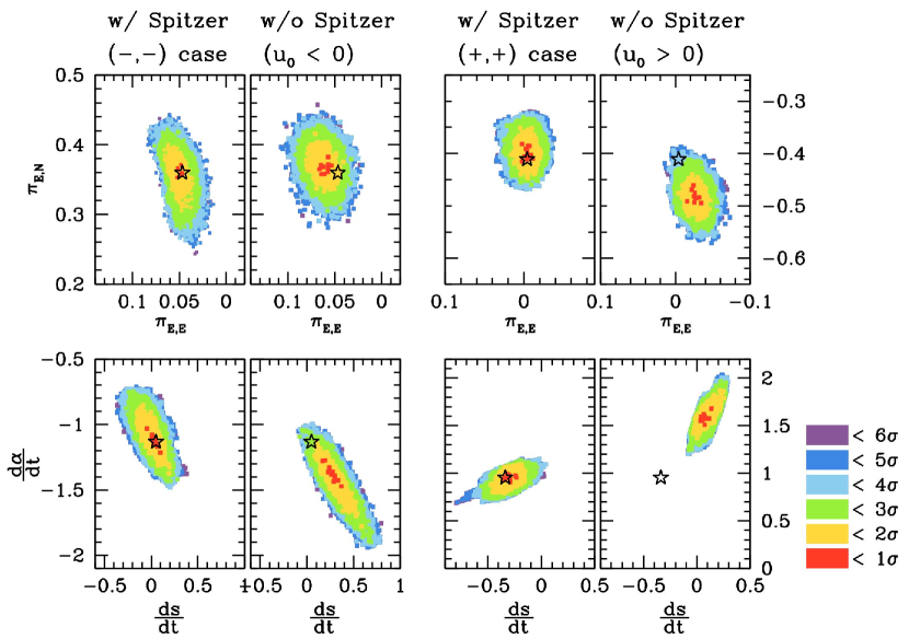
Figure 3.— The distributions of the microlens parallax and lens orbital motion parameters. Left panels show $(-,-)$ and $(u_{0}<0)$ cases of the MCMC chain scatters with and without the Spitzer data. Red, yellow, green cyan, blue, and purple colors represents $\Delta\chi^{2}$ between the best-fit and chain value less than $1,2,3,4,5,$ and $6\sigma$, respectively. The star represents the best-fit value of the model including the Spitzer data. Right panels show $(+,+)$ and $(u_{0}>0)$ cases with an identical scheme to the right panels.

3.3. Modeling of Spitzer lightcurve

For this test, we conduct modeling of the combined ground and Spitzer observations. We present observed lightcurves with the best-fit models in Figure 1. During the modeling process, we investigate degenerate solutions caused by the “four-fold degeneracy” (Zhu et al., 2015). The degeneracies are caused by different source trajectories seen by ground and space telescopes passing over a similar lensing magnification pattern, which is reflected over the binary axis. The degenerate solutions are denoted by the combination of the signs of impact parameters as seen from the space and ground, i.e., $(\pm,\pm)$, according to the conventional way (see Section 3 in Zhu et al., 2015). Under our parameterization, we can control the source trajectories by changing the sign of $u_{0}$ and $\pi_{{\rm E},{\it N}}$ parameters and thus we carefully set initial values to search for these models. For this event, we find that the $(-,-)$ and $(+,+)$ models showed similar fits with $\Delta\chi^{2}\sim 36.4$. However, there do not exist plausible local minima of the $(+,-)$ and $(-,+)$ solutions .

The observed Spitzer lightcurve is fragmentary and does not cover the caustic-crossing parts. Thus, we expect “color constraints” might be important to find the correct model including the Spitzer lightcurve (described in Section 5.3 of Yee et al., 2015a). To incorporate the color constraints, we use the (I-H, I) CMD described in Section 4.4 to find $(I-L)_{18}=5.157\pm 0.124$ where the subscript $18$ indicates a magnitude system for which $1$ flux unit corresponds to $18$th magnitude. We then introduce the “$\chi^{2}_{\rm penalty}$” defined as

$$\chi^{2}_{\rm penalty}\equiv{\left\{2.5\log(F_{\rm S,{\it Spitzer}}/F_{\rm S,OGLE})-(I-L)_{18}\right\}^{2}\over{\sigma_{\rm cc}^{2}}}$$ (2)

where $F_{\rm S,{\it Spitzer}}$ and $F_{\rm S,OGLE}$ are the source fluxes of each observatory, (i.e. of each passband) conducted from the model. The $\sigma_{\rm cc}$ is the uncertainty of the color constraints. The $\chi^{2}_{\rm penalty}$ increases according to increasing of the difference between the model-conducted color and color constraints. Note that, for the technical purpose, we additionally increase the penalty defined as

$$(\chi^{2}_{\rm penalty})^{\prime}={\rm fac}^{2}\times(\chi^{2}_{\rm penalty})$$ (3)

$$~{}~{}if~{}~{}2.5\log\left({F_{\rm S,{\it Spitzer}}\over F_{\rm S,OGLE}}\right)>\pm{\rm fac}\times\sigma_{\rm cc}(I-L)_{18}$$ (4)

where “${\rm fac}$” is a factor set as $2$. It implies that we use $(\chi^{2}_{\rm penalty})^{\prime}$ that is $4$ times lager than $\chi^{2}_{\rm penalty}$ if the color difference is lager than $2\sigma$ level of the color constraints.

In Table 2, we present the best-fit parameters of models both with and without the color constraints. The total $\chi^{2}$ consists of the sum of the $\chi^{2}$ for the ground-based data and the $\chi^{2}$ for the Spitzer data; the $\chi^{2}$ from the color constraint is given separately. For the analysis of this event, we find that the color constraints are of minor importance to the model. In fact, when fitting without the constraints, the model parameters are recovered within $3\sigma$ of those of the best-fit model with the constraints. Especially, the model parameters of the microlens parallax and the lens-orbital effect are recovered within $2\sigma$ level. Even though the color constraints play a relatively minor role, we conclude the best-fit models of this event are the cases of models considering the color constraints (bold parameters in Table 2). Because the color constraint is both an intrinsic observable and model-independent, the fact that the best-fit models satisfy these constraints serves as an independent check that they correspond to the physical system.

4. Results

4.1. Breaking the degeneracy of the microlens parallax

For the case of the OGLE-2016-BLG-0168 event, we found that two possible solutions $(-,-)$ and $(+,+)$ out of the possible four-fold degeneracy for the microlens parallax. The $\Delta\chi^{2}$ between those models is $\sim 36.4$, $10.9$ of which comes from $\Delta\chi^{2}_{\it Spitzer}$. In addition, we found inconsistency between the prediction of the lightcurve covered by the Spitzer data made from the ground-based data alone for the $(u_{0}>0)$ solution and the best-fit model including Spitzer data for the $(+,+)$ solution, as indicated by the different curvatures of the Spitzer lightcurve seen in Figure 2. Furthermore, for the prediction of the $(+,+)$ case, there exist large inconsistencies in the parameters between the $(u_{0}>0)$ ground-only model and the model including Spitzer data for the $(+,+)$ case at the $4\sigma$ and more than $6\sigma$ levels for the microlens parallax and lens-orbital parameters, respectively (see Figure 3). Hence, considering all the clues to resolve the degeneracy, we conclude the $(-,-)$ model is the unique solution that describes the nature of the binary lens system of this lensing event.

4.2. Confirmation of the annual microlens parallax

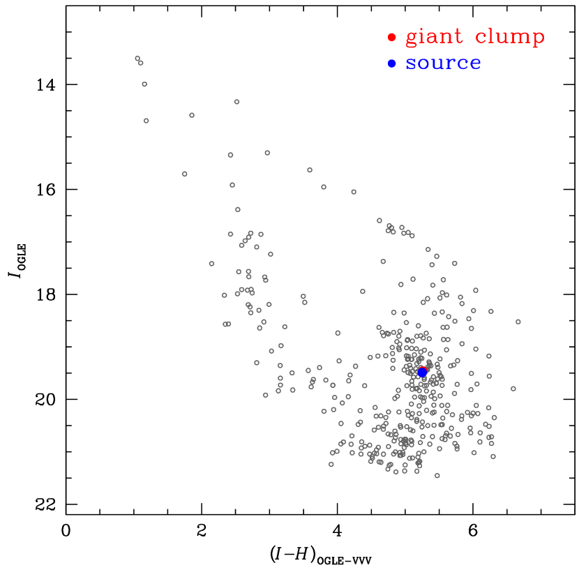
Figure 4.— (${\it I-H,I}$) Color Magnitude Diagrams of OGLE-2016-BLG-0168 event. The CMD is constructed by cross-matching OGLE and VVV data. Red and blue dots indicate the positions of the centroid of giant clump and the source star, respectively.

As shown in Figure 2, for the $(-,-)$ case, the prediction is almost the same as the lightcurve found by including the Spitzer data in the fitting. Thus, the higher-order effects measured from the ground-based lightcurve alone are confirmed by the Spitzer observations. Note that the prediction of the space-based lightcurve is dominated by the microlens parallax parameters. However, the microlens parallax parameters are strongly affected by the lens-orbital effect (Shin et al., 2012). Thus, the lens-orbital parameters are also essential factors for the successful prediction of the Spitzer lightcurve.

In Figure 3, we present distributions of the microlens parallax and lens-orbital parameters to clearly show the confirmation of the prediction for the ($(-,-)$ and $(u_{0}<0)$) case. We find that parameters of the ground $(u_{0}<0)$ model that are used for the prediction are well matched to those of the model including Spitzer data for the $(-,-)$ case, i.e. within $2\sigma$ and $3\sigma$ for the microlens parallax and lens-orbital parameters, respectively.

4.3. Value of fragmentary Spitzer observations

The confirmation of the microlens parallax and the resolution of the $(-,-)$–$(+,+)$ degeneracy show that it is possible to extract valuable information from space-based observations even though the observations are fragmentary. Although this is one specific case, it is significant because almost all space-based observations have only partial coverage of long time-scale lensing events. Thus, we frequently encounter such fragmentary lightcurves.

4.4. Properties of the binary lens system

Based on the unique best-fit model, it is then possible to specifically determine the properties of the binary lens system. To determine the properties, the angular Einstein ring radius and the microlens parallax are essential information. Thanks to good caustic coverage from KMTNet observations, we can clearly detect the signal of the finite source effect. From the measurement of $\rho_{\ast}=\theta_{\ast}/\theta_{\rm E}$, it is possible to determine the angular Einstein ring radius, $\theta_{\rm E}$. The angular source radius, $\theta_{\ast}$, can be determined from the position of the source on the CMD of the event. The conventional method is to use the (V-I, I) CMD, but this is impossible in this case because the source suffers from severe extinction ($A_{I}=4.9$).

We construct an (I-H, I) CMD from the OGLE survey and the VISTA Variables and Via Lactea Survey (VVV: Minniti et al., 2010) by cross-matching field stars within $60^{\prime\prime}$ of the source. Based on the CMD (see Figure 4), the centroid of giant clump, which is the reference to measure the extinction toward the source, is $({\it I-H,I})_{\rm clump}=(5.26,19.46)$. The position of the source on the CMD is determined as follows. First, from the best-fit model, we have ${\it I}_{\rm S,OGLE}=19.49$. Second, based on SMARTS CTIO I- and H-band data and converting from $(I_{\rm CTIO}-H_{\rm CTIO})$ to $(I_{\rm OGLE}-H_{\rm 2MASS})$ using comparison stars, we find $({\it I-H,I})_{\rm S}=(5.25,19.49)$. As shown in Figure 4, the locations of the source and the centroid of the red giant clump are almost identical. By adopting the intrinsic color and magnitude of the centroid of giant clump (Bensby et al., 2013; Nataf et al., 2013) and applying the conventional method (Yoo et al., 2004), we determine the de-reddened color and brightness of the source as $({\it V-I,I})_{\rm 0,S}=(1.05,14.55)$. Finally, the angular source radius, $\theta_{\ast}=5.66\pm 0.40$, is determined by converting $({\it V-I})$ to $({\it V-K})$ based on the color-color relation in Bessell & Brett (1988), and then the angular radius of the source is determined by using the color/surface-brightness relation in Kervella et al. (2004).

Table 3The properties of the binary lens system

quantity	value
Einstein radius, $\theta_{\rm E}$ (mas)	1.429 $\pm$ 0.103
Total Mass, $M_{\rm total}$ $(M_{\odot})$	0.484 $\pm$ 0.050
Primary Mass, $M_{1}$ $(M_{\odot})$	0.274 $\pm$ 0.028
Secondary Mass, $M_{2}$ $(M_{\odot})$	0.210 $\pm$ 0.022
Distance to lens, $D_{\rm L}$ (kpc)	1.572 $\pm$ 0.140
Projected separation, $a_{\perp}$ (AU)	2.480 $\pm$ 0.221
Geocentric proper motion, $\mu_{\rm geo}$ (mas/yr)	5.573 $\pm$ 0.402
Heliocentric proper motion, $\mu_{\rm hel}$ (mas/yr)	6.314 $\pm$ 0.456
Stability of system, $KE/PE^{\dagger}$	0.514

Note. — $\dagger~{}$ If the ratio of the Kinetic to Potential energy of the binary lens system $(KE/PE)$ is less then $1$, then the orbital motion of binary components is physically allowed. However, values $(KE/PE)\sim 1$ and values $(KE/PE)\ll 1$ would require very special physical configurations and/or viewing angles. Hence, the parameters of the model considering the lens-orbital effect are quite reasonable values.

Based on the location on the CMD and the intrinsic color of the source, the spectral type of the source an early K-type giant. We adopt limb-darkening coefficients based on the classified source type (Claret, 2000). The coefficient for I-band is equal to $\Gamma_{\it I}=(2u/(3-u))=0.5103$ where $u_{\it I}=0.6098$ under assumptions of the properties of the early K-type giant: effective temperature, $T_{\rm eff}\sim 4750$ K, metallicity, $[M/H]\sim 0.0$, turbulence velocity, $V_{\rm t}<2.0~{}{\rm km/s}$, and surface gravity, $\log{g}\sim 2.0$.

Combining the information of the microlens parallax and the angular Einstein ring radius, we can determine the properties of the binary lens system according to the equations (1). In Table 3, we present the properties of the lens system. The system consists of nearly equal mass stars,

$$M_{1}=0.27\pm 0.03~{}M_{\odot};~{}M_{2}=0.21\pm 0.02~{}M_{\odot},$$ (5)

with a projected separation,

$$a_{\perp}=2.48\pm 0.22~{}{\rm AU}.$$ (6)

The lens system is located $1.57\pm 0.14$ kpc from us.

Since we introduce orbital motion of the lens system, we check whether the best-fit orbital parameters are physically reasonable or not. Thus, we derive the ratio of kinetic to potential energy of the system to validate the stability of the lens system. The determined value $(KE/PE)\simeq 0.5$ easily satisfies the physically bound condition $(KE/PE)<1$. Moreover, it is well away from the regimes $(KE/PE)\sim 1$ and $(KE/PE)\ll 1$, both of which would require special geometries and/or viewing angles. Since, systematic-induced modeling errors would tend to generate arbitrary values of $(KE/PE)$, the fact that the modeling yields a value in the “typical range”, is further confirmation of its correctness. This is important in the present case because lens is unusually close ($D_{L}=1.6\,$kpc) and the orbital motion is usually fast $(|d\alpha/dt|\sim 1\,{\rm radian\,yr^{-1}})$. A number of the most interesting microlensing events, e.g. OGLE-2011-BLG-0417 (Shin et al., 2012), OGLE-2011-BLG-0420 and OGLE-2009-BLG-151 (Choi et al., 2013), are from such nearby lenses, which are intrinsically relatively rare but which frequently permit ground-based parallax measurements when they occur. Hence, when one of these can be verified as a physically (rather than systematics) generated lightcurve by several independent checks, it enhances confidence in this entire interesting class of events.

In Figure 5, we present the cumulative distribution of the “distance parameter”, $D_{8.3}$ (see Section 5 of Calchi Novati et al., 2015a), of published microlensing events with well-measured $\pi_{\rm rel}\,(=\pi_{\rm E}\theta_{\rm E})$ based on Spitzer observations. We note that the lens system of this work is the nearest one with a Spitzer distance. Assuming that 2-body lenses, which dominate this sample, follow the same galactic distribution as all lenses, this distribution represents the most precise determination of the Spitzer-observed lens distance distribution, a key factor in understanding the distribution of planets in out galaxy.

5. Summary and Discussion

We analyzed the microlensing event OGLE-2016-BLG-0168 based on combined ground- and space-based observations obtained from OGLE, KMTNet, and Spitzer telescopes. It is possible to clearly detect signals of higher-order effects in the lightcurve which are caused by the finite source, the microlens parallax, and the orbital motion of the binary lens components. Based on the additional information from these high-order effects, we found that this event is created by a binary system consisting of almost equal mass M-dwarf stars ($\sim 0.27$ and $\sim 0.21$ $M_{\odot}$) with a projected separation $\sim 2.5$ AU. The system is located $\sim 1.6$ kpc from us.

We successfully predict the Spitzer lightcurve of the $(-,-)$ model case based on the annual microlens parallax measured by using the ground-based observations. The annual microlens parallax is confirmed at the $2\sigma$ level by the satellite microlens parallax measured with Spitzer observations. In addition, it is possible to resolve the degenerate solutions by using the Spitzer observations.

Figure 5.— Cumulative distribution of $D_{8.3}$ of Spitzer microlensing events. We adopted $\pi_{\rm rel}$ value from published result of each case: OB141050 (Zhu et al., 2015), OB150196 (Han et al., 2017), OB150479 (Han et al., 2016b), OB150763 (Zhu et al., 2016), OB150966 (Street et al., 2016), OB151268 (Zhu et al., 2016), OB151285 (Shvartzvald et al., 2015) OB151319 (Shvartzvald et al., 2016), OB151482 (Chung et al., 2017), and OB161195 (Shvartzvald et al., 2017).

Our test of the microlens parallax can provide an important example for preparing for the new era of microlensing technique in collaboration with space-based observations. In principle, the microlensing technique can detect a variety of astronomical objects regardless of their brightness. However, additional observables are required to reveal what kind of object produces the microlensing event. Among these essential observables, the microlens parallax is one of the key pieces of information that reveals the nature of the lens of the event. Thus, it is important to routinely and securely measure the microlens parallax. Before the collaboration with space-based observations, measuring the microlens parallax usually depended on the time-scale of the lensing event. For some lensing events with long time-scale, the microlens parallax signal can be detected. However, this annual microlens parallax might be inaccurately measured due to systematics in the data. With the commencement of the era of space-based observations collaboration, however, the microlens parallax can be routinely measured regardless of the time-scale and magnification level of the lensing event.

Since most space-based observations cover only part of the full lensing lightcurves with a long time-scale due to the relatively short observing window, it is important to conduct a test to determine whether it is possible to extract secure information of the microlens parallax or not. In addition, since space-based observations can provide a chance to resolve degenerate solutions, it is also important to conduct another test to determine whether the degeneracy breaking is possible or not by using fragmentary space-based observations.

We conduct the microlens parallax test by using the fragmentary Spitzer observation of OGLE-2016-BLG-0168 binary lensing event. Our testing result provides an example showing that it is possible to verify the microlens parallax and resolve the degeneracy based on space-based observations, even though the observation is fragmentary. This result will be helpful for preparing collaboration of ground microlens surveys and space telescopes and next-generation microlensing survey on the space such as Spitzer microlensing campaign (Yee et al., 2015b), K2C9 (Henderson et al., 2016), and WFIRST (Spergel et al., 2015).

References

- Alard & Lupton (1998) Alard, C. & Lupton, Robert H. 1998, ApJ, 503, 325
- Albrow et al. (2009) Albrow, M. D., Horne, K., Bramich, D. M., et al. 2009, MNRAS, 397, 2099
- An (2005) An, Jin H. 2005, MNRAS, 356, 1409
- Batista et al. (2011) Batista, V., Gould, A., Dieters, S., et al. 2011, A&A, 529, A102
- Bensby et al. (2013) Bensby, T., Yee, J. C., Feltzing, S., et al. 2013, A&A, 549, 147
- Bessell & Brett (1988) Bessell, M. S., & Brett, J. M. 1988, PASP, 100, 1134
- Bond et al. (2001) Bond, I. A., Abe, F., Dodd, R. J., et al. 2001, MNRAS, 327, 868
- Bozza et al. (2016) Bozza, V., Shvartzvald, Y., Udalski, A. 2016, ApJ, 820, 79
- Calchi Novati et al. (2015a) Calchi Novati, S., Gould, A., Udalski, A., et al. 2015, ApJ, 804, 20
- Calchi Novati et al. (2015b) Calchi Novati, S., Gould, A., Yee, J. C., et al. 2015, ApJ, 814, 92
- Cardelli et al. (1989) Cardelli, J. A., Clayton, G. C., & Mathis, J. S. 1989, ApJ, 345, 245
- Choi et al. (2013) Choi, J.-Y., Han, C., Udalski, A., et al. 2013, ApJ, 768, 129
- Chung et al. (2017) Chung, S.-J., Zhu, W., Udalski, A., et al. 2017, ApJ, 838, 154
- Claret (2000) Claret, A. 2000, A&A, 363, 1081
- Dong et al. (2009) Dong, S., Gould, A., Udalski, A., et al. 2009, ApJ, 695, 970
- Dong et al. (2007) Dong, S., Udalski, A., Gould, A., et al. 2007, ApJ, 664, 862
- Dominik (1999) Dominik, M. 1999, A&A, 349, 108
- Graff & Gould (2002) Graff, D. S., & Gould, A. 2002, ApJ, 580, 253
- Griest & Safizadeh (1998) Griest, K., & Safizadeh, N. 1998, ApJ, 500, 37
- Gould (1992) Gould, A. 1992, ApJ, 392, 442
- Gould (1994) Gould, A. 1994, ApJ, 421, 71
- Gould (1997) Gould, A. 1997, ApJ, 480, 188
- Gould & Yee (2013) Gould, A., & Yee, J. C. 2013, ApJ, 764, 107
- Jiang et al. (2004) Jiang, G., DePoy, D. L., Gal-Yam, A., et al. 2004, ApJ, 617, 1307
- Jung et al. (2015) Jung, Y. K., Udalski, A., Sumi, T., et al. 2015, ApJ, 798, 123
- Kervella et al. (2004) Kervella, P., Bersier, D., Mourard, D., et al. 2004, A&A, 428, 587
- Kim et al. (2016) Kim, S.-L., Lee, C.-U., Park, B.-G., et al. 2016, JKAS, 49, 37
- Han et al. (2016a) Han, C., Udalski, A., Lee, C.-U., et al. 2016, ApJ, 827, 11
- Han et al. (2016b) Han, C., Udalski, A., Gould, A, et al. 2016, ApJ, 828, 53
- Han et al. (2017) Han, C., Udalski, A., Gould, A., et al. 2017, ApJ, 834, 82
- Henderson et al. (2016) Henderson, C. B., Poleski, R., Penny, M., et al. 2016, PASP, 128, 124401
- Minniti et al. (2010) Minniti, D., Lucas, P. W., Emerson, J. P., et al. 2010, NewA, 15, 433
- Miyake et al. (2012) Miyake, N., Udalski, A., Sumi, T., et al. 2012, ApJ, 752, 82
- Nataf et al. (2013) Nataf, D. M., Gould, A., Fouqué, P., et al. 2013, ApJ, 769, 88
- Poindexter et al. (2005) Poindexter, S., Afonso, C., Bennett, D. P., et al. 2005, ApJ, 633, 914
- Refsdal (1966) Refsdal, S. 1966, MNRAS, 134, 315
- Schlafly & Finkbeiner (2011) Schlafly, E.F. & Finkbeiner, D.P. 2011, ApJ, 737, 103.
- Shvartzvald et al. (2015) Shvartzvald, Y., Udalski, A., Gould, A., et al. 2015, ApJ, 814, 111
- Shvartzvald et al. (2016) Shvartzvald, Y., Li, Z., Udalski, A., et al. 2016, ApJ, 831, 183
- Shvartzvald et al. (2017) Shvartzvald, Y., Yee, J. C., Calchi Novati, S., et al. 2017, ApJ, 840, L3
- Shin et al. (2011) Shin, I.-G., Udalski, A., Han, C., et al. 2011, ApJ, 735, 85
- Shin et al. (2012) Shin, I.-G., Han, C., Choi, J.-Y., et al. 2012, ApJ, 755, 91
- Shin et al. (2013) Shin, I.-G., Sumi, T., Udalski, A., et al. 2013, ApJ, 764, 64
- Spergel et al. (2015) Spergel, D., Gehrels, N., Baltay, C., et al. 2015, arXiv:1503.03757
- Street et al. (2016) Street, R. A., Udalski, A., Calchi Novati, S., et al. 2016, ApJ, 819, 93
- Skowron et al. (2011) Skowron, J., Udalski, A., Gould, A., et al. 2011, ApJ, 738, 87
- Skowron et al. (2016) Skowron, J., Udalski, A., Kozłowski, S., et al. 2016, Acta Astron, 66, 1
- Udalski et al. (1994) Udalski, A., Szymański, M., Kaluzny, J., et al. 1994, Acta Astron., 44, 227
- Udalski et al. (2015a) Udalski, A., Szymański, M. K., Szymański, G. 2015, Acta Astron., 65, 1
- Udalski et al. (2015b) Udalski, A., Yee, J. C., Gould, A., et al. 2015, ApJ, 799, 237
- Udalski (2003) Udalski, A. 2003, Acta Astron., 53, 291
- Wozniak (2000) Wozniak, P. R. 2000, Acta Astron., 50, 421
- Wyrzykowski et al. (2016) Wyrzykowski, Ł., Kostrzewa-Rutkowska, Z., Skowron, J., et al. 2016, MNRAS, 458, 3012
- Yee et al. (2015a) Yee, J. C., Udalski, A., Calchi Novati, S., et al. 2015, ApJ, 802, 76
- Yee et al. (2015b) Yee, J. C., Gould, A., Beichman, C., et al. 2015, ApJ, 810, 155
- Yoo et al. (2004) Yoo, Jaiyul, DePoy, D. L., Gal-Yam, A., et al. 2004, ApJ, 603, 139
- Zhu et al. (2015) Zhu, Wei, Udalski, A., Gould, A., et al. 2015, ApJ, 805, 8
- Zhu et al. (2016) Zhu, Wei, Calchi Novati, S., Gould, A., et al. 2016, ApJ, 825, 60
- Zhu et al. (2017) Zhu, Wei, Udalski, A., Calchi Novati, S., et al. 2017, ApJ, submitted, arXiv:1701.05191