Fluctuation analysis of electric power loads in Europe: Correlation multifractality vs. Distribution function multifractality

Abstract

We analyze the time series of the power loads of the 35 separated countries publicly sharing hourly data through ENTSO-E platform for more than 5 years. We apply the Multifractal Detrended Fluctuation Analysis for the demonstration of the multifractal nature, autocorrelation and the distribution function fundamentals. Additionally, we improved the basic method described by Kanterhardt, et al using uniform shuffling and surrogate the datasets to prove the robustness of the results with respect to the non-linear effects of the processes. All the datasets exhibit multifractality in the distribution function as well as in the autocorrelation function. The basic differences between individual states are manifested in the width of the multifractal spectra and in the location of the maximum. We present the hypothesis about the production portfolio and the export/import dependences.

I Introduction

Recently unprecedented processes influenced the global economy; “globalization” as an integration of the global production system on one side and a slow but stable banishment of the national overlook of the markets - “liberalization” on the other side. The energy sector despite of its crucial importance and appropriate level of the government control was also influenced. In Europe, two joint markets, Nordpool and CE, have been established and the production of the electric energy is not necessarily produced and consumed within one country but local distributors are free to buy electric energy from abroad.

On the other hand, from the ecological point of view, the Kyoto protocol and the Doha amendment prescribe the governments to focus on renewable sources to assure transition to sustainable development. A general feature of the renewable sources in contrast to the classical sources is low yield as well as the fact that installations are placed far from the centers of consumption that creates problems of additional currents on the international scale, see e.g., key28 . We also note that each country has specific portfolio of the power plants and they operate to follow needs of consumers.

Electric grid is operated on national level by the Transmission System Operator (TSO) that controls a swift and effective flow of energy from the powerplants to the consumers. The process is based on the large quantities of data measured in real-time and instantaneous action is taken if necessary to balance the electric network to be proportional to consumption. Naturally, the process is influenced by deterministic trends as well as random effects, see key02 ; Harris_Electricity_markets .

In the framework of physics there was developed the Langevin equation describing a path of a particle in a random environment

$$\mathrm{d}X\left(t\right) = \mu\left(t,X\left(t\right)\right)\cdot\mathrm{d}t+\mathrm{d}W\left(t,X\left(t\right)\right),$$ (1)

where $\mu\left(t,X\left(t\right)\right)$ is the deterministic drift that stands for deterministic effects in electric power system, while $dW\left(t,X\left(t\right)\right)$ is a term representing noise depending on actual state $X\left(t\right)$ that reflects random effects within the electricity power grid. Analysis of Eq. 1 in the framework of Brownian motion has been done in Ref. key05 . Usual assumption on the properties of the noise is the Gaussian distribution and memorylessness $\langle X\left(t\right)\cdot X\left(t+\Delta t\right)\rangle\sim\delta\left(\Delta t\right)$ or short range memory $\langle X\left(t\right)\cdot X\left(t+\Delta t\right)\rangle\sim\exp\left(-\frac{\Delta t}{L_{c}}\right)$, where $L_{C}$ is a correlation length.

However, in the real systems the properties may not be always satisfied, e.g., the probability distribution is a non-Gaussian one. Even more, it may be fat-tailed and (or) the autocorrelation function posses long-range memory $\langle X\left(t\right)\cdot X\left(t+\Delta t\right)\rangle\sim\Delta t^{-\gamma}$, where $\gamma$ is the exponent of the power law, see Rangarajan_Ding_Long-Range_correlations . A typical field of the study where the theory was used represents a stock exchange, see key03 , where large datasets have been stored and prepared for analysis.

In recent decades computers were widely used for the time-series analysis and among the methods that are used belong the Detrended Fluctuation Analysis (DFA) and its derivation the Multifractal Detrended Fluctuation Analysis (MFDFA), see key06 ; key07 ; key23 ; key26 ; key27 . Historically it is derived from the R/S method used in the field of hydrology, see Ref. key29 . Recently the time series analysis has focused on the problem of the trends and its impact on the analysis, see Refs. key09 ; key36 ; key40 . The literature also contain a non-orthodox modification of the MFDFA, see Ref. key35 ; key12 as well as modification usable for analyzing the cross-correlations among the time series, see Ref. key40 ; key58 . We note that the literature also contains modification that goes beyond one dimension, see Ref. key60 .

Versatility of the method has been proved in a number of applications. Originally it was used to analyze the datasets in biophysics, see Refs. key14 ; key15 ; key23 but recently the method is employed in the number of the studies spanning from surface roughness via human gain and econophysics to earthquakes and clouds, see key08 ; key03 ; key11 ; key13 ; key20 ; key25 ; key37 ; key61 ; key62 ; key64 . Generally speaking, the method demonstrated extracts effectively the information about the scaling properties within the dataset and then the properties of the autocorrelation function.

Focusing on electroenergetics there is a number of the studies focusing either on electric power loads and prices of electricity, see Ref. key02 ; key16 ; key17 ; key41 ; key52 . Recently a competition of the teams that predict price or electric power loads has grown around the globe and they use various methods, see Refs. key42 ; key45 ; key46 . General weakness of number of studies is natural presence of oscillations that spoils correct estimation of the Hurst exponent. The gap was filled in kracik-lavicka:2016 .

In this study we would like to examine the datasets of the electric power loads in the countries of Europe. We intend to perform the MFDFA and we also plan to exploit various enhancements of the method to reveal properties of both the distribution and autocorrelation functions. Moreover we test how the properties of the functions are condensed among parameters – we intend to question multifractality of the datasets. Finally we compare functionality of the states by the multifractal properties.

The structure of the paper is as follows. Firstly, we describe the method used in the study. Then we exploit power of computers and show the results of the analysis. Finally, we come with the conclusions focusing on the stochastic properties of the datasets and then we compare power loads of the European countries.

II Methods

Figure 1: The electric power load of three countries of Europe (upper figure) and the signals modulated $X^{car}\left(i\right)$ on the carrying signal $X^{car}\left(i\right)$ after performing Step 1 (bottom figure) spanning period since Jan 1 2010 to Oct 31 2013. Red, green and blue curves are Germany, Italy and Norway respectively. We show the typical examples of the the electric power load of countries with respect to seasonality and inter-day and inter-week changes. Germany is an example of the strong seasonality with the strong inter-day and inter-week changes. Italy shows the strong inter-day and inter-week changes with the limited seasonality. Finally, Norway exhibits the strong seasonality with the limited inter-day and inter-week changes.

Figure 2: The test statistics for the selected countries of Europe. Its comparison with $\chi_{m}^{2}$-distribution at the $99\%$ significance level with the $m$ degrees of freedom to the test hypothesis of none autocorrelations (region $\left[0,\chi_{m}^{2}\left(0.99\right)\right]$).

Figure 3: Comparison of quantiles of stochastic part of the time series for selected countries of the Europe.

To analyze a timeserie $\left\{X\left(i\right)\right\}{}_{i=1}^{N}$ with $N$ datapoints, usually as a result of a measurement of a physical variable, we perform modification of the Multifractal Detrended Fluctuation Analysis (MFDFA). If the timeserie is non-stationary where the driving forces of the system are stronger than the fluctuations within them we propose a method that is based on the following 10 steps:

Fourier transform:

Firstly we preform the Fourier transform to detect presence of the carrier signal in the sample of the timeserie

$$\widehat{X}\left(\omega\right) = \frac{1}{\sqrt{N}}\sum_{j=1}^{N}X\left(j\right)\exp\left(-2\pi\cdot\mathbf{i}\cdot j\cdot\omega\right).$$ (2)

Generalizations of the Fourier transforms are described in Kilbas_Saigo_H_transforms ; Mathai_Hausbolt_Special_functions ; Glaeske_Prudnikov_Skornik_Operational_calculus ; Brichkov_Special_functions ; Beals_Wong_Special_Functions ; Davies_Integral_transforms ; Erdelyi_Higher_Transcendental_Functions ; Lebedev_Special_functions and they can be used to strengthen abilities of the method to the wavelets of various types. We note that corresponding inversion formula must be used below.

For the colored noise (fluctuations) the Fourier transform follows $\hat{X}\left(\omega\right)\sim|\omega|^{\beta}$ with a number of the additional peaks caused by the carrier signal upon the fluctuations are modulated. We decompose the signal into two components

$$\widehat{X}\left(\omega\right) = \widehat{X}^{fluc}\left(\omega\right)+\widehat{X}^{car}\left(\omega\right),$$ (3)

where $\widehat{X}^{fluc}\left(\omega\right)\sim|\omega|^{\beta}$ is the Fourier transform of the modulated signal and the Fourier transform of the carrier signal is $\widehat{X}^{car}\left(\omega\right)$ and it defines the profile average

$$X^{car}\left(j\right) = \frac{1}{\sqrt{N}}\sum_{\omega=1}^{N}\widehat{X}^{car}\left(\omega\right)\cdot\exp\left(2\pi\cdot\mathbf{i}\cdot j\cdot\omega\right).$$ (4)

Test of presence of autocorrelations

The first step of the procedure is to test of the presence of autocorrelation within the sample. We define the test statistics made of the modulated signal $X^{fluc}\left(i\right)$ as

$$Q_{AC}\left(m\right)=N^{2}\sum_{i=1}^{m}\frac{C_{i}^{2}}{N-i},$$ (5)

where the sample autocorrelation is defined by formula

$$C_{i}=\frac{\sum_{k=i+1}^{N}X^{fluc}\left(k\right)\cdot X^{fluc}\left(k-i\right)}{\sum_{k=1}^{N}X^{fluc\ 2}\left(k\right)}.$$ (6)

The test statistics $Q_{AC}\left(m\right)$ follows $\chi_{m}^{2}$ with $m$ degrees of freedom if none autocorrelations are present in the sample. We fix the level of significance $\alpha$ and varying $m$. If $Q_{AC}\left(m\right)<\left(\chi_{m}^{2}\right)^{-1}\left(\alpha\right)$, where $\left(\chi_{m}^{2}\right)^{-1}\left(\alpha\right)$ stands for $\alpha$-th quantile of $\chi_{m}^{2}$ distribution , at the significance level $\alpha$ we conclude independence of $x_{k}$s for the segment of length $m$. In the opposite case $Q_{AC}\left(m\right)>\left(\chi_{m}^{2}\right)^{-1}\left(\alpha\right)$ the hypothesis of none autocorrelations is rejected.

We admit that the step is optional and it serves as an indicator of the presence of autocorrelations for the Gaussian distribution. The indicator for the non-Gaussian distribution would need to derive appropriate $\chi_{m}^{2}$ distribution.

Construction of profile

Construction of a profile $X^{prof}\left(i\right)$ of the timeserie from the modulated signal $X^{fluc}\left(i\right)$ is performed by formula

$$X^{prof}\left(i\right)=\sum_{j=1}^{i}X^{fluc}\left(i\right).$$ (7)

The step is auxiliary and it helps to perform the analysis accurately even for the anti-persistent processes. Please, see Ref. key06 for the discussion.

Separation into segments

We separate the profile of the timeserie $X^{prof}\left(i\right)$ into the $N_{s}$ windows $X^{seg,w}\left(i\right)$ covering the whole dataset with the length $s$ where each window is denoted by a number $w$. The minimal number of the windows is $\lfloor\frac{N}{s}\rfloor$, where $\lfloor x\rfloor$ is the largest integer smaller than or equal to a number $x$. Thus the number of the timesteps $N$ is not generally multiple of $s$. In order to obtain better statistics we use as small overlap of the consecutive windows where possible.

Construction of trend

We establish the local polynomial trend $X^{prof,w}\left(i\right)$ within each window $w$ of the size $s$ using the least square fit of the dataset. Using the trend we detrend the data and we calculate the sample variances in the window

$$F^{2}\left(s,w\right)=\frac{1}{s}{\displaystyle{\textstyle\sum}}_{i=1}^{s}\left(X^{seg,w}\left(i\right)-X^{prof,w}\left(i\right)\right)^{2},$$ (8)

where the calculation is performed for the windows $w=1,\ldots,N_{s}$.

Calculation of fluctuation function

The fluctuation function of the $q$-th order is defined by the formula:

$$F_{q}\left(s\right) = \begin{cases}q\neq 0&\frac{1}{2N_{s}}\sum_{w=1}^{2N_{s}}\left(F^{2}\left(s,w\right)^{\frac{q}{2}}\right)^{\frac{1}{q}}\\ q=0&\exp\left(\frac{1}{4N_{s}}\sum_{w=1}^{2N_{s}}\ln\left(F^{2}\left(s,w\right)\right)\right)\end{cases}.$$ (9)

Calculation of generalized Hurst exponent

The fluctuation function behaves as

$$F_{q}\left(s\right) \sim s^{h\left(q\right)+1},$$ (10)

where $+1$ correction stands for the correction to the integrated time series in $Step\ 2$. Generally, for positive $q$, $h\left(q\right)$ describes scaling behavior of large fluctuations within a segment while for negative $q$, $h\left(q\right)$ describes scaling behavior of small fluctuations. Independence $h\left(q\right)$ of $q$ means monofractal behavior of the dataset. If we assume that the fluctuations in the dataset are stable and follow the Gaussian distribution then the Hurst exponent $H=h\left(q=2\right)$ is then $0<H<1$ for the Gaussian distribution of the noise. For $H=\frac{1}{2}$, long range autocorrelation is not present and the dataset may be independent. $H>\frac{1}{2}$ means long-range autocorrelations (persistence) and $H<\frac{1}{2}$ stands for long range anti-autocorrelations (anti-persistence).

The non-Gaussian distributions with the power-law tail allows the generalized Hurst exponent to exceed the range of $\left(0,1\right)$, see key60 and $h\left(q\right)$ is a nontrivial function of the variable $q$. It generally exhibits combination of the effects caused by the probability distribution and the autocorrelation function. In order to extract information on both we execute next two additional steps.

Shuffling the dataset

We shuffle the original timeserie $\left\{x\left(i\right)\right\}{}_{i=1}^{N}$ to form $\left\{x^{shuf}\left(i\right)\right\}_{i=1}^{N}$ using the Fisher–Yates algorithm, see Knuth_Volume_2 for the description and the historical note. By calculating the fluctuation function of the shuffled timeserie $F_{q}^{shuf}\left(s\right)$ performing steps through $1$ to $5$ we obtain the shuffled fluctuation function

$$F_{q}^{shuf}\left(s\right) = \overline{F_{q,\left\{x^{shuf}\left(i\right)\right\}}\left(s\right)},$$ (11)

where the averaging is executed for the different realizations of shuffling. Shuffling of the original timeserie destroys (if present) autocorrelations and thus the shuffled fluctuation function carries information about the distribution function. By analogy of Eq. 10, the shuffled fluctuation function behaves

$$F_{q}^{shuf}\left(s\right) \sim s^{h^{shuf}\left(q\right)+1},$$ (12)

where $h^{shuf}\left(q\right)$ called shuffled Hurst exponent describes the scaling behavior of the fluctuation function of the shuffled timeserie.

Correlation Hurst exponent

We define the autocorrelation Hurst exponent $h^{cor}\left(q\right)$ as follows:

$$h^{cor}\left(q\right)=h\left(q\right)-h^{shuf}\left(q\right).$$ (13)

The autocorrelation Hurst exponent contains information on the autocorrelation function of the timeserie $\left\{x\left(i\right)\right\}{}_{i=1}^{N}$. For $H^{cor}>0$ the timeserie is long range autocorrelated while for $H^{cor}<0$ there is long range anti-autocorrelated behavior. In case $H^{cor}=0$ the timeserie is either non-autocorrelated or short range autocorrelated.

Surrogate dataset

We perform additional test using the surrogate dataset. We intend to verify robustness of our conclusions with respect to the non-linear effects and the non-Gaussian features. The surrogate dataset conserves the autocorrelation function. Calculation of the surrogate dataset $\left\{x^{sur}\left(i\right)\right\}{}_{i=1}^{N}$ is obtained using the inverse Fourier transform of

$$\widehat{X}^{sur}\left(\omega\right) = \widehat{X}^{fluc}\left(\omega\right)\cdot\exp\left(\mathbf{i}\cdot Q\left(\omega\right)\right),$$ (14)

where $Q\left(\omega\right)$ is a IID random variable with uniform distribution within the range $\left[-\pi,\pi\right]$. After then the MFDFA is used on $\left\{x^{sur}\left(i\right)\right\}_{i=1}^{N}$ using the above steps from 4 to 8. We perform $50$ samples of the surrogate dataset and the surrogate fluctuation function is defined by formula

$$F_{q}^{sur}\left(s\right) = \overline{F_{q,\left\{x_{i}^{sur}\right\}}\left(s\right)}.$$ (15)

Analogically, the surrogate fluctuation function follows

$$F_{q}^{sur}\left(s\right) \sim s^{h^{sur}\left(q\right)+1},$$ (16)

where $h^{sur}\left(q\right)$ is the surrogate Hurst exponent.

Distribution Hurst exponent

The distribution Hurst exponent is defined by

$$h^{dist}\left(q\right)=h\left(q\right)-h^{sur}\left(q\right).$$ (17)

The distribution Hurst exponent contains information about the distribution function and its scaling properties.

Multifractal spectrum

The fundamental properties of the autocorrelation function and the distribution function of the time series can be studied using multifractal spectrum $f\left(\alpha\right)$ that is Legendre transform of scaling function $\tau\left(q\right)=q\cdot h\left(q\right)-1$

$$f\left(\pi\right) \equiv q\left(\pi\right)\cdot\pi-\tau\left(q\left(\pi\right)\right)$$ (18)

$$\pi \equiv \frac{d\tau}{dq}=q\cdot h^{\prime}\left(q\right)+h\left(q\right).$$ (19)

Since we deal with three generalized Hurst exponents ($h\left(q\right)$, $h^{cor}\left(q\right)$, $h^{shuf}\left(q\right)$) we calculate $f\left(\pi\right)$, $f^{cor}\left(\pi\right)$ and $f^{shuf}\left(\pi\right)$. In case that the autocorrelation function has monofractal property or the distribution function has single exponent then $\pi=const.$ For multifractal case there occurs a distribution of $\alpha$ values for both the autocorrelations as well as distributions, see Harte:2001 . The width of the spectrum $\triangle\pi=\pi_{max}-\pi_{min}$ describes the strength of multifractality, where $\pi_{max}=\max_{q}\pi\left(q\right)$ and $\pi_{min}=\min_{q}\pi\left(q\right)$. For broad spectrum $\triangle\pi$ is an indicator of strong multifractality while for narrow spectrum it is the indicator of weak multifractality of the time series.

Analogically the autocorrelation and distribution multifractal spectrums are defined by equations 18 and 19 with $h^{cor}\left(q\right)$ and $h^{dist}\left(q\right)$ respectively. They produce $f^{cor}\left(\pi\right)$ and $f^{dist}\left(\pi\right)$ and the widths of multifractal spectrums are $\Delta\pi^{cor}=\pi_{max}^{cor}-\pi_{min}^{cor}$ and $\Delta\pi^{dist}=\pi_{max}^{dist}-\pi_{min}^{dist}$.

Figure 4: The fluctuation function for the MFDFA-4 for France for $q\in\left\{-10,-5,-2,2,5,10\right\}$. Fluctuation functions are shifted by power of $10$ between each consecutive $q$. The typical power law behavior is presented.

Figure 5: The generalized Hurst exponents $h\left(q\right)$, $h^{shuf}\left(q\right)$ and $h^{cor}\left(q\right)$ are shown from top to bottom respectively. The orders of the MFDFA between $2$ to $6$ are plotted with various colors for United Kingdom (excluding Northern Ireland).

Figure 6: The multifractal spectrum $f\left(\pi\right)$, the shuffled multifractal spectrum $f^{shuf}\left(\pi\right)$ and the multifractal autocorrelation spectrum $f^{cor}\left(\pi\right)$ for Cyprus of the MFDFA orders between 2 and 7 is shown. The typical numerical issues can be observed at the bottom as the wings.

Figure 7: Plot of maxims of the autocorrelation multifractal spectrum for states or national authorities in Europe shown for various orders of the MFDFA from 2 to 7.

Figure 8: The width of the multifractal shuffled (on the top) and correlation (at the bottom) spectrum calculated by the MFDFA-4 and it is visualized on the map of Europe.

Figure 9: Comparison of the widths of the correlated and shuffled multifractal spectrums. The order of the MFDFA is indicated by different symbol. Square, circle and triable down are the orders 4,5 and 6 respectively.

III Results of analysis

We perform the methodology which was described in the previous section on a dataset of the electric power load for 35 European countries or the independent electric power systems which were obtained from ENTSO-E . This organization roofs local Transmission System Operators (TSO) that control the swift and effective functionality of the backbone electric power grid in the European countries. The dataset spans from January 1 2008 to December 31st 2012 with the one-hour resolution for the longest dataset.

Each measured datapoint collects produced electricity within a region as it counts for exports, imports and adding balance of pumped-storage hydroplants . It amounts electric power that is provided to users – citizens, industry and services – through local electric distribution companies. We also note that actual demand that is intended to be satisfied must be lower in longer periods of time than actual supply, otherwise blackout can happen on small or on the larger scale. To prevent significant economic and physical waste of electric power companies producing and transmitting electric power are trying to correlate both variables to the extent possible. We may also perceive the dataset as a measure of an activity (economic, social) of a society. Autocorrelations of the datasets can be understood as an indicator of autocorrelations in European countries that share data through ENTSO-E.

III.1 Oscillations in power grid data

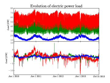
Firstly, we show examples of datasets of typical European countries at the top of the Fig. 1. Each dataset exhibits oscillations of period a year, a week and a day but the countries differ in proportions of the oscillations on the time scale. Countries of the south Europe usually exhibit limited one-year oscillations in contrast to the countries of the northern Europe. Since most of the countries are of Christian origin, the religious holidays are usually public holidays, e.g., Christmas and Easter. There is a significant decrease of the electric power load during that period. Oscillations can generally spoil the results of MF-DFA and biasing statistical analysis, see key09 ; key36 . Performing Step 1 of the method we obtain a dataset (signal) that is modulated on the carrying signal. We note that performing cuts during Step 1 have been tested for different exponents $\beta$ with minimal qualitative impact on results of following analysis, see kracik-lavicka:2016 .

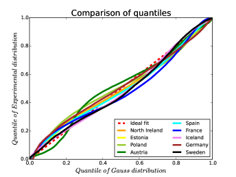
We show examples of the modulated signal for Germany, Italy and Norway at the bottom of the Fig. 1. The modulated signal $\left\{X^{fluc}\left(i\right)\right\}_{i=1}^{N}$ is then analyzed and tested for the presence of autocorrelations or types of distribution. We performed Komogorov-Smirnov test of the signal and rejected null hypothesis that there is the Gaussian distribution, e.g. for Norway the p-value stands at extremely small value $\thicksim 10^{-290}$ and for Germany at $\thicksim 10^{-105}$ so that it fails to reject the null hypothesis. To demonstrate deviations from the Gaussian distribution, see Fig. 3. The power loads of the countries deviate from diagonal line and the deviations show the presence of the asymmetric probability distribution. Due to the fact that Austria does not fit the pattern of the rest of the states we suppose that it is due to diverge portfolio of the power plants.

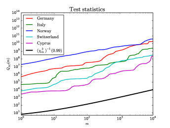
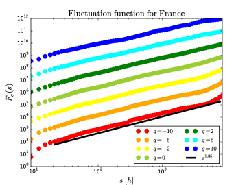
Secondly we perform an autocorrelation test of a dataset, calculating $Q_{AC}\left(m\right)$ and comparing with $\chi_{m}^{2}$ distribution at $99\%$ level of significance. In the Fig. 2, the test rejects hypothesis of no-autocorrelation within a sample dataset for each European country. It motivates taking the following steps of the methodology that aims at the calculation of the MF-DFA to reveal properties of the autocorrelation and distribution function. Via performing steps from 4 to 8 and 10 we obtain $F_{q}\left(s\right)$, $F_{q}^{shuf}\left(s\right)$ and $F_{q}^{sur}\left(s\right)$ that follows the power laws 10, 12 and 16, which is for France demonstrated in the Fig. 4.

III.2 MFDFA

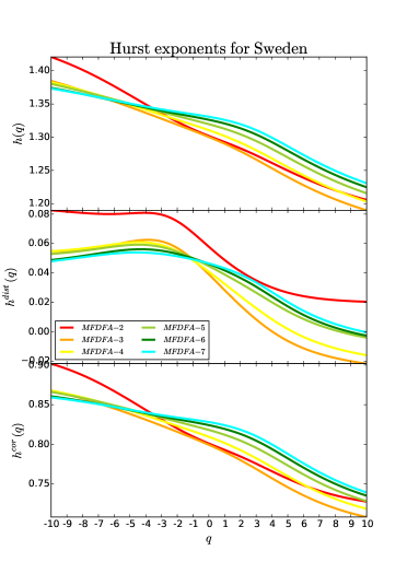
The calculation of the appropriate Hurst exponents $h\left(q\right)$, $h^{shuf}\left(q\right)$ and $h^{sur}\left(q\right)$ is then a key point for calculation $h^{cor}\left(q\right)$ and $h^{dist}\left(q\right)$ (steps 9 and 11) that contain information on the scaling properties of the autocorrelation and distribution function. For illustration, we show $h\left(q\right)$, $h^{dist}\left(q\right)$ and $h^{cor}\left(q\right)$ in the Fig. 5 for Sweden. We note that the generalized Hurst exponent $h\left(q\right)$ is estimated above standard range for the Gaussian distribution $\left[0,1\right]$ . Next $h^{dist}\left(q\right)$ is close to $0$ indicating that the non-linear effects does not spoil Hurst exponent estimation. Finally, the autocorrelation Hurst exponent $h^{cor}\left(q\right)$ indicates a presence of multifractality for autocorrelation function.

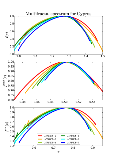
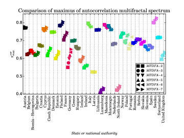
Next, we focus on multifractal spectrums defined by Eqs. 18 and 19, the multifractal spectrum $f\left(\pi\right)$, the shuffled multifractal spectrum $f^{shuf}\left(\pi\right)$ and the autocorrelation multifractal spectrum $f^{cor}\left(\pi\right)$ that are shown in Fig. 6 for Cyprus. All spectrums exhibit a peak-like structure with the most frequent value $\pi_{max}$, $\pi_{max}^{shuf}$ and $\pi_{max}^{cor}$ respectively, forming the top of the appropriate multifractal spectrum. In table 1 we show $\pi_{max}^{shuf}$ for the states of Europe and it is mostly close to $\frac{1}{2}$, indicating the most frequent presence of the Gaussian distribution. However, maximums of the autocorrelation multifractal spectrum $\pi_{max}^{cor}$ varyes significantly from one country to another, see the Fig. 7. $\pi_{max}^{cor}$ is also out of standard range $\left[-\frac{1}{2},\frac{1}{2}\right]$ for the Brownian processes except for North Ireland, Luxembourg and Latvia that is on the edge. Most frequently the process is governed by 1 and the stochastic process is persistent. However, the other states are governed by the most frequent process described by equation

$$\mathrm{d}\dot{X}\left(t\right) = \mu\left(t,\dot{X}\left(t\right)\right)\cdot\mathrm{d}t+\mathrm{d}W\left(t,\dot{X}\left(t\right)\right).$$ (20)

The maximum of the autocorrelation multifractal spectrum is then deceased by 1 (Similarly when we skip to execute step 2 but execute steps 7,8 and 10 as they are). The process is then anti-persistent, similar analysis in Ref. key41 also revealed anti-persistent processes within the power grids. While the$2$nd order differential equations are more stable with respect to the observation of displacement of particles at the start and at the end than the $1$st order equations and the weaker anti-persistence also decreases deviations. We argue that higher $\pi_{max}^{cor}$ is more beneficial for stability of the electric power grids.

III.3 Multifractal spectra

We also report that the wide multifractal spectrums are present within the dataset, see Tab. 1. Since the width of the autocorrelation multifractal spectrum $\triangle\pi^{cor}$ is wider, we conclude that multifractality of autocorrelation function is also stronger than the distribution function. Since the width of the distribution multifractal spectrum $\bigtriangleup\pi^{dist}$ is far smaller than $\triangle\pi^{cor}$ and $\triangle\pi$ and $\pi_{max}^{dist}$ is close to zero, we conclude that the non-linear effects are limited. Nevertheless they are present and multifractality is not a side effect but it has a systematic nature in the operation of the electric power system. We admit that the width of the distribution and correlation spectrums is usually influenced by the numerical issues, see the bottom of the Fig. 6.

III.3.1 Operational properties of power grids in Europe

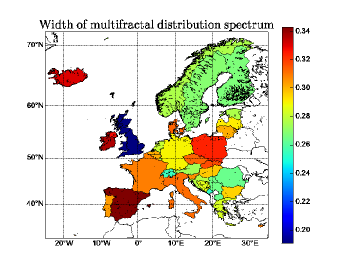
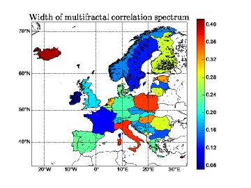
Focusing on the operational properties of the national power grids, we demonstrate the differences in the Fig. 8 by metric of the width of the shuffled and autocorrelation multifractal spectrums. North-South or East-West spatial clustering based on political or climatic is not present for both spectrums. The widest widths of the shuffled multifractal spectrums is present for North Ireland, Spain and a cluster of states in the central Europe, namely Germany, Poland, Czech Republic and Slovakia. Interestingly, the cluster is investigated in Ref. key28 from the point of view of the trans-border flows reveals enormous production of the electric energy from the wind power plants in north Germany and consumption in south Germany with the enormous cross-border electric power traffic spanning Poland, Czech Republic and Slovakia.

The autocorrelation multifractal spectrum is usually wider than the shuffled one. We observe central block of countries with relatively narrow spectrum where countries with wider spectrum are placed randomly. The widest spectrum is present for Iceland, Poland, Estonia and Spain while the narrowest spectrum is present for France, Latvia and Bulgaria. We refer reader to the Table 1 where results of MFDFA for order 4 are presented.

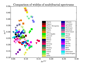
We show the space of the widths of the shuffled and autocorrelation multifractal spectrums in the Fig. 9. Most states operate within an elliptic cluster with center at $\left(0.2,0.2\right)$ a semi-axes $\left(0.05,0.1\right)$ with few deviations like Iceland, Latvia, Spain and Poland which operate with much wider spectrums. Additionally North Ireland, Latvia, Luxembourg and to some degree additional states develop, due to their location of maximums of the autocorrelation spectrum $\pi_{max}^{cor}$ close to $\frac{1}{2}$ and considerable widths of spectrums, Formulas 1 and 20.

III.4 Clusterization of the states

Figure 10: The renormalized values of various widths of the multifractal spectra are shown and compared for order 5 of the method. On left hand side we present clusterization of the states in euclidean metric.

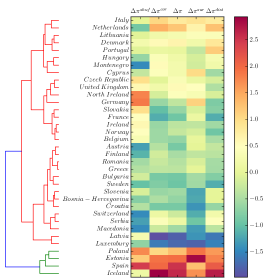
We employed Machine learning tools to search for clusters to put out previous observations of clusterization on solid ground, see Python_data_science_essentials ; pedregosa2011scikit ; Learning_scikit_learn ; Introduction_Machine_Learning . Since the widths of multifractal spectra are order dependent the clusters presence vary and more than 2 clusters were observed for orders 2, 3 and 4 for different methods of clusterization, metric and subset of the widths of spectra.

Most countries of Europe operate power grid systems in the region with a limited variety of Hurst exponents, see red cluster in Fig. 10. The deviations are present and that are namely Iceland, Spain, Estonia and Poland(only for the order 5). However, we observed additional presence of Germany, Czech Republic, Slovakia, Portugal and North Ireland for different setup of clusterization algorithm. For Iceland, portfolio of sources of electricity is widely different than in the rest of Europe. Presence of Germany, Czech Republic, Slovakia a Poland in deviating group may be caused by crossborder transfer in cetral Europe, see key28 .

III.5 Note on implementation and robustness of results

We note that we performed the analysis for various orders of the method with minimal impact on the conclusions. In the table 1 we report the complete multifractal analysis of European countries including the widths of all multifractal spectrums as well as the locations of the maxims of all multifractal spectrums for order 4 of the MFDFA.

The method have been implemented in Zarja library with appropriate Python interface. Python is then used for post-processing of the datasets. During the analysis we employed Matplotlib Hunter:2007 , Basemap, SciPy Scipy , NumPy and Scikit tools pedregosa2011scikit ; Learning_scikit_learn . The analysis using the MFDFA gives the best results for orders 4, 5 and 6. The lower orders lacks effective detrending but electic power grids are relatively stable in this respect.

On the other hand, we also admit that the analysis can be inaccurate for both large $|q|$ and the high orders of the MFDFA. It is caused by use of floating point numbers (IEEE 754) that are inaccurate, see Knuth_Volume_2 , due to the fixed length of the data-type. To solve the problem we refer to the use the fractions or to the variable length numbers, however the use is at the expense of the speed. Implementing MFDFA can solve the problem.

IV Conclusions

We performed the modification of the MFDFA method on the dataset obtained from the electric power grid of the European countries which consists of two level of detrending. Dataset analyzed are the electric power loads with one hour frequency. In the study we focus on the properties of the autocorrelation function and the probability distribution of the stochastic process governing evolution of the system.

To address whether the properties of the distribution and autocorrelation function are unique or more parameters are involved we employ multifractal spectrum of the autocorrelation and distribution function. All countries admit multifractality of both the autocorrelation and distribution functions. To be more specific, all datasets admit existence of the non-Gaussian probability distribution due to the width of multifractal spectra as well as the long-range autocorrelation function.

We detected presence of the countries that posses the parameters that Langevin equation for both the coordinates and the velocities have to be employed. Generally, we verified the robustness of our analysis performing the surrogated datasets as well as various orders of detrending and no non-linear effects spoils the analysis. The low orders of detrending seems to be inefficient and too high orders are influenced by numeric instability but the main message is robust.

The analysis of the spatial properties of the noise within the electric grids among the states does not differ so much. The properties of the distribution function among the states are practically the same but the differences are present for the autocorrelation function. Few states possess the most frequent description by the derivatives of the power load and the weak anti-persistent process. Few states (Luxembourg, Latvia and North Ireland) follow the strong persistent process of the electric power loads and most states follow description by the derivatives and strong anti-persistent process. The wide width of the multifractal spectrums is mostly scattered among Europe except for the cluster of central European countries where the width of the shuffled multifractal spectrum can be understood as an effect of the imbalance due to installations of the wind power plants in north Germany. The problem should be also addressed more closely using different datasets. Interesti

The wide width of the autocorrelation multifractal spectrum is scattered on the map of Europe. Since it is present for Iceland we believe that it shall be related to the hidden connection with the structure of the power production. We emphasize that more analysis of the wider set of datasets is needed.

To put the paper in the context of the analysis of the time series and particularly in the analysis electric electric grids, we exploited widely used methodology and improved it with the additional tests and detrending method. We performed deep analysis of stochastic properties of the time series for European countries that goes beyond trends and we address the properties of the noise and its effective description by Langevin equation.

Practically, in the long horizon, the study shall be useful for unbiased description of the electric power grids using the stochastic processes and the effective handling of the risk management. Based on the analysis we focus on use of the Fractionally integrated autoregressive conditional heteroscedastic processes (FIARCH), see Granger-Ding:1996 ; Rangarajan_Ding_Long-Range_correlations or Autoregressive fractionally integrated moving average process (ARFIMA) key70 ; Hosking1981 ; Granger-Joyeux:1980 that are able to generate the time series with the power-law correlations for prediction of the electric power loads. Recently, generalization of both processes is proposed in Podobnik-et-all:2005 for symmetric distribution functions. However, our previous study kracik-lavicka:2016 revealed that the distribution function is asymmetric even more it may not fit to any element from the set of the Lévy stable distributions, see key55 ; key70 ; Podobnik-et-all:2005 . It supports a hypothesis that the poles of the Mellin transform, see Kilbas_Saigo_H_transforms , of the distributions are not stationary.

Author contributions

J.K. obtained and prepared the dataset. J.K and H.L. developed the main ideas of the paper. H.L. prepared the tool for analysis for UNIX-like system. Both authors also performed literature search, the analysis of the time series and the visualization of the results. J.K and H.L both contributed to the writing of the manuscript and the work was performed under H.L. leadership. The work described in this paper will be used in J.K.’s Ph.D. thesis.

	Widths of multifractal spectrum					Position of maxima
Country	$\Delta\pi$	$\Delta\pi^{shuf}$	$\bigtriangleup\pi^{sur}$	$\bigtriangleup\pi^{cor}$	$\bigtriangleup\pi^{dist}$	$\pi_{max}$	$\pi_{max}^{shuf}$	$\pi_{max}^{sur}$	$\pi_{max}^{cor}$	$\pi_{max}^{dist}$
Austria	0.370	0.175	0.362	0.216	0.102	1.266	0.494	1.232	0.772	-0.018
Belgium	0.383	0.215	0.373	0.199	0.099	1.123	0.499	1.110	0.624	-0.029
Bosnia-Herzegovina	0.363	0.190	0.310	0.184	0.095	1.137	0.493	1.116	0.644	-0.008
Bulgaria	0.378	0.199	0.335	0.192	0.064	1.121	0.500	1.120	0.621	-0.010
Croatia	0.374	0.199	0.304	0.176	0.071	1.169	0.497	1.154	0.672	0.010
Cyprus	0.461	0.199	0.412	0.290	0.089	1.255	0.495	1.279	0.760	-0.017
Czech Republic	0.426	0.227	0.380	0.209	0.090	1.133	0.501	1.122	0.632	-0.021
Denmark	0.487	0.208	0.359	0.300	0.155	1.240	0.495	1.217	0.745	0.022
Estonia	0.559	0.226	0.487	0.383	0.185	1.113	0.498	1.138	0.605	-0.093
Finland	0.374	0.179	0.341	0.209	0.099	1.283	0.497	1.293	0.786	-0.053
France7	0.371	0.210	0.367	0.169	0.057	1.227	0.495	1.223	0.724	-0.037
Germany	0.432	0.249	0.415	0.225	0.085	1.087	0.502	1.091	0.583	-0.023
United Kingdom	0.404	0.216	0.368	0.194	0.071	1.126	0.499	1.138	0.620	-0.045
Greece	0.408	0.196	0.341	0.215	0.092	1.195	0.492	1.177	0.703	-0.001
Hungary	0.458	0.196	0.352	0.286	0.148	1.158	0.493	1.126	0.665	0.033
Ireland	0.386	0.219	0.333	0.186	0.085	1.060	0.494	1.061	0.565	-0.002
Iceland	0.570	0.201	0.434	0.417	0.214	1.090	0.496	1.088	0.597	-0.030
Italy	0.433	0.200	0.387	0.271	0.146	1.278	0.498	1.236	0.780	0.003
Latvia	0.351	0.213	0.302	0.143	0.058	1.018	0.496	1.017	0.521	0.000
Lithuania	0.457	0.202	0.387	0.275	0.138	1.257	0.497	1.228	0.760	0.014
Luxembourg	0.356	0.186	0.269	0.178	0.092	0.951	0.494	0.973	0.460	-0.010
Macedonia	0.387	0.174	0.308	0.219	0.086	1.283	0.489	1.265	0.794	0.028
Montenegro	0.377	0.169	0.335	0.213	0.111	1.268	0.491	1.249	0.762	-0.063
Netherlands7	0.498	0.182	0.390	0.341	0.171	1.183	0.495	1.160	0.688	0.035
Northern Ireland	0.381	0.246	0.357	0.149	0.080	0.952	0.500	0.954	0.450	-0.049
Norway	0.369	0.214	0.339	0.166	0.075	1.231	0.494	1.257	0.736	-0.060
Poland	0.536	0.249	0.469	0.340	0.187	1.196	0.502	1.141	0.694	-0.040
Portugal	0.466	0.203	0.339	0.284	0.179	1.175	0.496	1.146	0.679	0.046
Romania	0.409	0.191	0.361	0.230	0.108	1.183	0.495	1.169	0.688	-0.032
Serbia	0.396	0.175	0.315	0.229	0.107	1.204	0.494	1.197	0.709	-0.013
Slovakia	0.385	0.223	0.364	0.180	0.092	1.183	0.500	1.167	0.683	-0.024
Slovenia	0.388	0.198	0.299	0.200	0.107	1.157	0.495	1.131	0.662	0.026
Spain7	0.574	0.258	0.396	0.354	0.209	1.169	0.504	1.131	0.665	0.038
Sweden	0.402	0.180	0.325	0.224	0.079	1.300	0.494	1.331	0.807	-0.027
Switzerland	0.390	0.175	0.310	0.226	0.114	1.214	0.500	1.204	0.714	0.014

Table 1: Collection of results of the MFDFA analysis of the order $4$.

References

- (1) Z. Boldiš, “Czech electricity grid challenged by German wind,” Europhys. News, vol. 44, no. 4, pp. 16–18, 2013.
- (2) R. Weron, Modeling and Forecasting Electricity Loads and Prices: A Statistical Approach. John Wiley and Sons Ltd, 2006.
- (3) C. Harris, Electricity markets: Pricing, Structures and Economics. John Wiley and Sons Ltd, 2006.
- (4) G. E. Uhlenbeck and L. S. Ornstein, “On the theory of brownian motion,” Phys.Rev., vol. 36, pp. 823–841, 1930.
- (5) G. Rangarajan and M. Ding, eds., Processes with long-range correlations, vol. 621. Springer-Verlag Berlin Heidelberg, 2003.
- (6) R. Mantegna and H. Stanley, An introduction to econophysics: correlations and complexity in finance. New York, NY, USA: Cambridge University Press, 2000.
- (7) J. Kantelhardt, S. Zschiegner, E. Koscielny-Bunde, S. Havlin, A. Bunde, and H. Stanley, “Multifractal detrended fluctuation analysis of nonstationary time series,” Physica A, vol. 316, p. 87, 2002.
- (8) J. Kantelhardt, E. Koscielny-Bunde, H. Rego, S. Havlin, and A. Bunde, “Detecting long-range correlations with detrended fluctuation analysis,” Physica A, vol. 295, p. 441, 2001.
- (9) C.-K. Peng, S. Havlin, H. E. Stanley, and A. L.Goldberger, “Quantification of scaling exponents and crossover phenomena in nonstationary heartbeat time series,” Chaos, vol. 5, pp. 82–87, 1995.
- (10) A. L. Goldberger, L. A. N. Amaral, L. Glass, J. M. Hausdorff, P. C. Ivanov, R. G. Mark, J. E. Mietus, G. B. Moody, C.-K. Peng, and H. E. Stanley, “PhysioToolkit, and PhysioNet: Components of a new research resource for complex physiologic signals,” Circulation, vol. 101, pp. e215–e220, 2000.
- (11) C.-K. Peng, J. Mietus, J. M. Hausdorff, S. Havlin, H. E. Stanley, and A. L. Goldberger, “Long-range anticorrelations and non-gaussian behavior of the heartbeat,” Phys. Rev. Lett, vol. 70 (9), pp. 1343–1346, 1993.
- (12) H. E. Hurst, “Long term storage capacity of reservoirs,” Trans. Am. Soc. Civ. Eng., vol. 116, no. 770, 1951.
- (13) K. Hu, P. C. Ivanov, Z. Chen, P. Carpena, and H. E. Stanley, “Effect of trends on detrended fluctuation analysis,” Phys. Rev. E, vol. 64, p. 011114, 2001.
- (14) Z. Wu, N. E. Huang, S. R. Long, and C. K. Pen, “On the trend, detrending, and variability of nonlinear and nonstationary time series,” PNAS, vol. 104, no. 38, pp. 14889–14894, 2007.
- (15) D. Horvatic, H. E. Stanley, and B. Podobnik, “Detrended cross-correlation analysis for non-stationary time series with periodic trends,” Europhys. Lett., vol. 94, no. 18007, 2011.
- (16) C. V. Chianca, A. Ticona, and T. J. P. Penna, “Fourier-detrended fluctuation analysis,” Physica A, vol. 357, pp. 447–454, 2005.
- (17) X.-Y. Qian, G.-F. Gu, and W.-X. Zhou, “Modified detrended fluctuation analysis based on empirical mode decomposition for the characterization of anti-persistent process,” Physica A, vol. 390, pp. 4388–4395, 2011.
- (18) B. Podobnik and H. E. Stanley, “Detrended cross-correlation analysis: A new method for analyzing two nonstationary time serie,” Phys. Rev. Lett., vol. 100, no. 084102, 2008.
- (19) G.-F. Gu and W.-X. Zhou, “Detrended fluctuation analysis for fractals and multifractals in higher dimensions,” Phys. Rev. E, vol. 74, no. 061104, 2007.
- (20) C.-K. Peng, S. V. Buldyrev, S. Havlin, M. Simons, H. E. Stanley, and A. L. Goldberger, “Mosaic organization of DNA nucleotides,” Phys. Rev. E, vol. 49, pp. 1685–1689, 1994.
- (21) C.-K. Peng, S. V. Buldyrev, A. L. Goldberger, S. Havlin, F. Sciortino, M. Simons, and H. E. Stanley, “Long-range correlations in nucleotide sequence,” Nature, vol. 356, pp. 168–170, 1992.
- (22) T. Preis, P. Virnau, W. Paul, and J. J. Schneider, “Accelerated fluctuation analysis by graphic cards and complex pattern formation in financial markets,” New J. Phys., vol. 11, p. 093024, 2009.
- (23) A. Bunde, S. Havlin, J. W. Kanterhardt, T. Penzel, J. H. Peter, and K. Voigt, “Correlated and uncorrelated regions in heart-rate fluctuations during sleep,” Phys. Rev. Lett., vol. 85, pp. 3736–3739, 2000.
- (24) P. Talkner and R. O. Weber, “Power spectrum and detrended fluctaution analysis: Application to daily temperatures,” Phys. Rev. E, vol. 64, pp. 150–160, 2000.
- (25) T. Preis, W. Paul, and J. J. Schneider, “Fluctuation patterns in high-frequency financial asset returns,” Europhys. Lett., vol. 82, p. 68005, 2008.
- (26) J. W. Kantelhardt, Y. Askenazy, P. C. Ivanov, A. Bunde, S. Havlin, T. Penzel, J.-H. Peter, and H. E. Stanley, “Characterization of sleep stages by correlations in the magnitude and sign of heartbeat increments,” Phys. Rev. E, vol. 051908, 2002.
- (27) K. Koçak, “Examination of persistence properties of wind speed records using detrended fluctuation analysis,” Energy, vol. 34, pp. 1980–1985, 2009.
- (28) S. Hosseinabadi and M. Rajabi, “Stochastic and fractal properties of silicon and porous silicon rough surfaces,” J. of Phys.:Conf. ser., vol. 454, no. 012035, 2013.
- (29) D. Stauer and D. Sornette Physica A, vol. 252, no. 271, 1998.
- (30) K. Ivanova and M. Ausloos, “Application of the detrended fluctuation analysis (dfa) method for describing cloud breaking,” Physica A, vol. 274, no. 1-2, p. 349, 1999.
- (31) R. Weron and A. Przybylowicz, “Hurst analysis of electricity price dynamics,” Physica A, vol. 283, 2000.
- (32) R. Weron, “Energy price risk management,” Physica A, vol. 285, p. 127, 2000.
- (33) I. Simonsen, “Measuring anti-correlations in the nordic electricity spot market by wavelets,” Physica A, vol. 322, pp. 597–606, 2003.
- (34) P. Norouzzadeh, W. Dullaert, and B. Rahmani, “Anti-correlation and multifractal features of spain electricity spot market,” Physica A, vol. 380, pp. 333–342, 2007.
- (35) S. Chan, K. Tsui, H. Wu, Y. Hou, Y.-C. Wu, and F. Wu, “Load/price forecasting and managing demand response for smart grids: Methodologies and challenges,” IEEE Signal Processing Magazine, pp. 68 – 85, 2012.
- (36) T. Hong, P. Pinson, and S. Fan, “Global energy forecasting competition 2012,” Int. J. Forecasting, vol. 30, no. 2, pp. 357–363, 2014.
- (37) R. Weron, “Electricity price forecasting: A review of the state-of-the-art with a look into the future,” Int. J. Forecasting, vol. 30, pp. 1030–1081, 2014.
- (38) J. Kracík and H. Lavička, “Fluctuation analysis of high frequency electric power load in the czech republic,” Physica A: Statistical Mechanics and its Applications, vol. 462, pp. 951 – 961, 2016.
- (39) A. A. Kilbas and M. Saigo, H-Transforms: Theory and Application, vol. Analytical methods and special functions of An International Series of Monographs in Mathematics. Chapman and Hall, 2004.
- (40) A. Mathai and H. Hausbolt, Special Functions for Applied Scientists. Springer, 2008.
- (41) H. Glaeske, A. Prudnikov, and K.A.Skórnik, Operational Calculus and Related Topics, vol. Analytical methods and special functions of An International Series of Monographs in Mathematics. Chapman and Hall, 2006.
- (42) Y. A. Brychkov, Handbook of Special Functions, Derivatives, Integrals, Series and Other Formulas. CRC Press, 2008.
- (43) R. Beals and R. Wong, Special Functions. Cambridge University Press, 2010.
- (44) B. Davies, Integral Transforms and Their Applications. Springer, 2002.
- (45) W. Magnus, F. Oberhettinger, and F.G.Tricomi, Higher Transcendental Functions, vol. III. McGraw-Hill Book Company, 1953.
- (46) N. Lebedev, Special Functions nad Their Applications. Translation from Russian Prentice-Hall, 1965.
- (47) , where is incomplete Gamma function.
- (48) D. Knuth, The Art of Computer Programming-Seminumerical Algorithms (Third Edition), vol. 2. Addison-Wesley, 1997.
- (49) D. Harte, Multifractals: Theory and applications. Chapman and Hall, 2001.
- (50) Web page http://www.entsoe.eu.
- (51) The datasets does not include electric power production for local needs – powerplants for a factory or a house – and also power production within islands disconnected from the mainland.
- (52) Then the autocorrelation Hurst exponent defined by Eq. 13 is in range .
- (53) Well, Latvia is just at the border.
- (54) A. Boschetti and L. Massaron, Python Data Science Essentials. Packt Publishing, 2015.
- (55) F. Pedregosa, G. Varoquaux, A. Gramfort, V. Michel, B. Thirion, O. Grisel, M. Blondel, P. Prettenhofer, R. Weiss, V. Dubourg, J. Vanderplas, A. Passos, D. Cournapeau, M. Brucher, M. Perrot, and E. Duchesnay, “Scikit-learn: Machine Learning in Python,” Journal of Machine Learning Research, vol. 12, pp. 2825–2830, Oct. 2011.
- (56) R. Garreta and G. Moncecchi, Learning scikit-learn: Machine Learning in Python. Packt Publishing, 2013.
- (57) A. Müller and S. Guido, Introduction to Machine Learning with Python. O’Reilly Media, 2017.
- (58) http://sourceforge.net/projects/zarja/.
- (59) J. D. Hunter, “Matplotlib: A 2d graphics environment,” Computing In Science & Engineering, vol. 9, no. 3, pp. 90–95, 2007.
- (60) E. Jones, T. Oliphant, P. Peterson, et al., “SciPy: Open source scientific tools for Python,” 2001–. [Online; accessed 2017-01-30].
- (61) C. Granger and Z.Ding, “Varieties of long-range memory models,” J. Econometr., vol. 73, pp. 61–77, 1996.
- (62) G. Samorodnitsky and M. S. Taqqu, Stable Non-Gaussian Random Processes: Stochastic Models with Infinite Variance. Chapman and Hall, New York, 1994.
- (63) J. R. M. Hosking, “Fractional differencing,” Biometrika, vol. 68, no. 1, pp. 165–176, 1981.
- (64) C. Granger and R. Joyeux, “An introduction to long-memory time series models and fractional differencing,” J. Time Ser. Anal., vol. 1, no. 15, pp. 15–29, 1980.
- (65) B. Podobnik, P. C. Ivanov, K. Biljakovic, D.Horvatic, H.E.Stanley, and I.Grosse, “Fractional integrated process with power-law correlations in variables and magnitudes,” Phys. Rev. E, vol. 026121, 2005.
- (66) K.-I. Sato, Lévy Processes and Infinitely Divisible Distributions. Cambridge University Press, 1999.