A new stochastic
STDP Rule
in a neural Network Model
Abstract
Thought to be responsible for memory, synaptic plasticity has been widely studied in the past few decades. One example of plasticity models is the popular Spike Timing Dependent Plasticity (STDP). There is a huge litterature on STDP models. Their analysis are mainly based on numerical work when only a few has been studied mathematically. Unlike most models, we aim at proposing a new stochastic STDP rule with discrete synaptic weights. It brings a new framework in order to use probabilistic tools for an analytical study of plasticity. A separation of time-scale enables us to derive an equation for the weights dynamics, in the limit plasticity is infinitely slow compare to the neural network dynamic. Such an equation is then analysed in simple cases which show counter intuitive result: divergence of weights even when integral over the learning window is negative. Finally, without adding constraints on our STDP, such as bounds or metaplasticity, we are able to give a simple condition on parameters for which our weights’ process remains ergodic. This model attempts to answer the need for understanding the interplay between the weights dynamics and the neurons ones.
1 Introduction
A huge amount of studies have focused on neural networks dynamics in order to reproduce biological phenomena observed in experiments. Thereby, there exist many different individual neuron models from the two states neurons to the adaptive exponential integrate-and-fire [24, 17]. Compare to this kind of literature, plasticity in recurrent networks has been well less studied. One reason is because it adds an additional layer of complexity to existing models despite being a candidate for memory formation, learning, etc [10, 6].
In the beginning, plasticity models were based on firing rates [8]. Later on, as suggested by Hebb’s in 1949 [23], the crucial role of precise spikes timings was proved experimentally and gave rise to Spike-Timing Dependent Plasticity (STDP) [36, 7, 34]. Following such a breakthrough, numerous STDP models emerged. They were associated with neural networks of either Poisson neurons [29, 30, 18] or continuous model of neurons [1, 12, 40].
Here, we would like to present a new STDP rule which
is implemented in the well-known stochastic Wilson-Cowan model of spiking neurons as presented in [5]. More precisely, because of the plasticity rule, our model is a piecewise deterministic Markov process [13, 14] whereas it is a pure point process in [5].
Motivations for proposing such a new model are four folds. First, although mechanisms involved in plasticity are mainly stochastic such as the activation of ions channels and proteins, the majority of studies on STDP are implemented using a deterministic description or an extrinsic noise source [38, 12, 21]. One exception is the stochastic STDP model proposed by Appleby and Elliott in [3, 4]. The stochasticity of their model lies in the learning window size. They analyse
the dynamic of the weights of one target cell innervated by a few Poisson neurons. A fixed point analysis enabled them to show that their model is not relevant in the pair-based case and that multispike interactions are required to get stable competitive weights dynamics. Second, most studies are based on simulations and their analyses, thus there is still a need to find a good mathematical framework, see [16, 33, 40]. We propose here a mathematical analysis based on probabilistic methods which leads to a control of weights through the study of their dynamics on their slow time scale. Indeed, long term plasticity timescale ranges from minutes to more than one hour. On the other hand, a spike lasts for a few milliseconds [38]. Thus, third, there is a need to understand how to bridge this time scale gap between the synapse level and the network one[15, 48, 45]. Finally, the interplay between the weights dynamics and the neurons ones is not yet fully understood and we think the study of recurrent networks is necessary to bring some basis to fully numerical studies.
Such motivations impose some constraints on our model. It has to be rich enough to reproduce biological phenomena, simple enough to be mathematically tractable and easily simulated with thousands of neurons. Finally, it has to enable us to observe macroscopic effects out of microscopic events. The Wilson-Cowan model has been widely studied [9, 5, 33] and reproduces many biological features of a network such as oscillation and bi-stability for example. On the other hand, based on experimental evidence [7, 44], we propose a new STDP rule with intrinsic noise with fixed synaptic weight increment [41]. This allows to control independently the synaptic weight increment and the probability of a plasticity event. Indeed, several pairs protocol are required for the induction of plasticity [7, 36].
Thus, we can produce a mathematical analysis by studying the Markov process composed of the following three components: the synaptic weight matrix, the inter-spiking times and the neuron states. In the context of long term plasticity, synaptic weights dynamics are much slower than the neural network one. A timescale analysis enables us to remove the neurons dynamics from the equations. Then we can derive an equation for the slow weights dynamics alone, in which neurons dynamics are replaced by their stationary distributions. Thus, we don’t need to simulate the dynamics of thousands of fast neurons and we obtain a much easier equation to analyse. We then discuss the implications of such derivation for learning and adaptation in neural networks.
A similar analysis has been done in a few papers with different mathematical tools and models [29, 30, 40, 18, 19, 32]. When the two first one studied only one postsynaptic neuron, the last ones had a look at recurrent networks. Thanks to a separation of time scale, they derive an equation for weights in which STDP appears in an integral of the STDP curve against cross-correlation matrix. The main problem is the computation of such a matrix, they use Taylor expansion and Fourier analysis to derive estimations of it. We don’t need such an estimation for our analysis thanks to probabilistic methods.
2 Presentation of the model and notations
As in all model of neural networks with plastic connections, one can separate the neuron model and the plasticity one. Our neuron model is the well-known stochastic Wilson-Cowan model of spiking neurons presented in [5]. In such a model, neurons are binary, meaning they are either at rest, state 0, or spiking, state 1.
This model has been widely studied in the case of fix weights and presents realistic features such as oscillations or bistable phenomenon, see [9]. However, there are only few studies with plasticity, see for instance with an Ising model in [42].
We implement plasticity in this model in a stochastic way. Indeed, our plasticity rule depends on the precise spike times and thus has the same form as STDP, see [35] for an overview, but is not deterministic: in the situation of correlated spikes, weights will change or not according to a certain probability.
First, we are interested in excitatory neurons, as in most models inhibitory neurons are not plastic, so the synaptic weights will be positive. Also, we suppose they are all to all connected so this positivity will be strict. We will discuss about these assumptions at the end. Therefore, we first give some global notations, then explain the neuron model, the plasticity rule, and finally we gather these dynamics in the generator of the process.
We are interested in analysing the time continuous Markov process where:
-
-
synaptic weights matrix, , and , weight of the connection from neuron to at t.
-
-
vector of times from last spikes of neurons.
-
-
neuron system state.
As weights dynamics and the neural network one will be separated, we spare the global state space in two spaces. Hence, in the following we denote , such that .
Neuron model
Let’s define the dynamic of the process. It is a recurrent neural plastic network with Poisson neurons in interaction. Each neuron jumps with an inhomogeneous rate between two states: 0 and 1. This rate depends on the network state and the weights matrix:
| (1) |
Where is given by bounded, positive and nondecreasing:
| (2) |
As the neuron activity is never null, we will consider that for all , . Hence, is uniformly bounded in and for all :
Plasticity rule
The basic idea of STDP is that of the Hebb’s law (1949):
“When an axon of cell A[…] repeatedly or persistently takes part in firing (a cell B), […]A’s efficiency, as one of the cells firing B, is increased” [23].
STDP is a bit more complex as it completes this law with the possibility for weights to decrease when they are decorrelated.
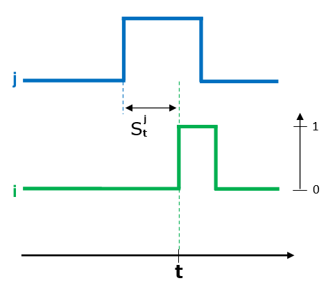
We expose our plasticity model through an example. First, weights can change only when a neuron spikes that we define as the jump from 0 to 1 (we could have chosen from 1 to 0
. So suppose the neuron spikes at time . Then, weights related to this neuron, that is to say and for all , have a certain probability to jump. This differs from models we can find in the literature for which weights’ jumps are systematic but small [29, 1, 38]. Here, the jump is not small but happens with a small probability: has probability to increase and decrease with probability . These probabilities depends on the inter-spiking times given by :
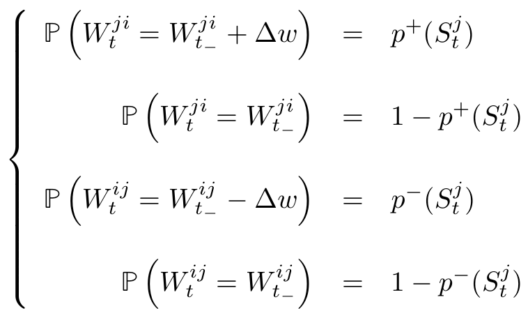
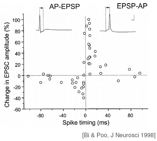
As the classic STDP curve, found by Bi&Poo [7], suggests it, we take the following probability functions in our examples, with and :
| (3) |
Remark 1.
By definition of and , we study excitatory neurons. We see at the end how to extend our results to inhibitory-excitatory neurons. Also, we remark that stays constant and as for all , for all . We will discuss this assumption later on. Finally, is crucial for our process to be Markovian.
Generator of the process
Now we know how the process works, we can write its infinitesimal generator. To do so, we need the following notations. We denote by all reachable weights after a spike of neuron while the current weight is . Thus:
Where
We call (respectively ) the matrix associated to the vector (respectively ). As each weight jumps independently whenever a neuron spikes, we can decompose the probability of jumping to a certain state as the product of probabilities to jump or not for each weights. We want to compute , the probability of jumping in a given knowing the neuron spikes. Let , the probability for to increase () is when the probability to stay the same () is , for all . This will appear as in :
| (4) |
Therefore, we can write the generator of the all process where and given :
Or
Written in this form, the generator shows two different dynamics which are related: the weights dynamic and the network, inter-spiking time dynamics. As we know that synaptic weights dynamics are slow compare to the network dynamics ( change fast compare to ), this means that for all :
Typically, and . This time scale difference is studied in section 3.2 while the study of the fast part of the process is done in section 3.1. This process is given by the generator :
| (5) |
3 Derivation of the weight equation
3.1 Invariant measure of the fast processes
In this section, is fixed. We are interested in proving:
Theorem 3.1.
For all , the process with generator mapping into , defined as:
| (6) | ||||
| (7) | ||||
| (8) |
has a unique invariant measure.
This aim enters in a bigger ambition to analyse the total process on two different time scales. Indeed, in the limit where the plasticity is infinitely slow, it stays constant so , and then for all , . This analysis enables us to show in section 3.2 that, on the slow time scale of plasticity, behaves simply against the invariant measure of . In the following, we omit the dependence on in the notation of processes only and we use instead of .
In a first subsection we show existence of an invariant measure of the process and then its uniqueness in the next subsection. We start with some notations.
Notations
Let with and . The process is then the same as the one defined before with a fixed matrix of weights . Each , for , follows the same kind of process: the discrete variable jumps with a total rate when . Between these jumps, the continuous part will grow linearly with a slope of 1 () except when jumps from 0 to 1 at time , then the continuous part restarts from 0, i.e. , see .
From these notations, one can denote by the counting process corresponding to the number of jump of the process . We can then define the processes where are counters of the number of jumps of neuron i. By definition of , one has where are independent Poisson processes of intensity 1, as in [27]. Finally, we call the transition probability of the process, maps in . Hence, for all (-algebra of Borel sets of ), is the probability that knowing , probability also written as .
3.1.1 Existence using a Lyapounov function
In this subsection, we aim at proving the following theorem:
Proposition 3.2.
The process defined in Theorem 3.1 has at least one invariant measure of probability.
To do so, we use the following theorem, classical in theory of discrete Markov chains on any state space:
Theorem 3.3.
If a transition probability P is Feller and admits a Lyapunov function, then it also has an invariant probability measure.
Proof.
A nice proof of this result can be found in the course of Martin Hairer called Ergodic Properties of Markov Processes. See theorem 2 of [46]. Just need to show condition () is equivalent to our Lyapunov condition. ∎
After recalling the definitions of a Lyapunov function and a Feller process, we find such a Lyapunov function for our process.
Definition 3.4.
Let X be a complete separable metric space and let P be a transition probability on X . A Borel measurable function is called a Lyapunov function for P if it satisfies the following conditions:
-
-
, in other words there are some values of for which is finite.
-
-
For every , the set is compact.
-
-
There exists a positive constant < 1 and a constant such that for every x such that :
Definition 3.5.
We say that a homogeneous Markov process with transition operator P is Feller if Pf is continuous whenever f is continuous and bounded. It is strong Feller if Pf is continuous whenever f is measurable and bounded.
We emphasize that previous definitions and theorem are given for Markov chains and not processes. The following proposition links them.
Proposition 3.6.
Let be a Markov semigroup over X and let for some fixed . Then, if is invariant for P, the measure defined by:
is invariant for .
Proof.
∎
Hence, we want to apply theorem 3.3 to the transition probability extracted from for some fixed .
To do so, we show that for any given time, defined as is a Lyapunov function for . Then we use theorem 27.6 of the Davis’ book [14] to prove is Feller. We conclude on the existence of the invariant measure of probability for and thus for thanks to proposition 3.6.
After these definitions and notations, let’s prove the process has at least one invariant measure , i.e. or more formally, :
| (9) |
Existence
Assumption 3.7.
such that :
Proposition 3.8.
With assumption 3.7, for any , is Lyapunov for with constants and , .
Proof.
The main idea is to use the fact that values return to 0 whenever neuron jumps from 0 to 1. Hence, as neurons have only two states, if , neuron has jumped at least one time from 0 to 1 between and . Therefore, decomposing possible events we get:
So
∎
Furthermore, one can show the process is Feller thanks to Davis’ book [14]:
Proposition 3.9.
is Feller.
Proof.
First, we define a distance such that is a metric space, locally compact. Such a distance is proposed in [14] page 58:
| (10) | ||||
We need this kind of norm because if we take for instance the euclidean distance , we can have and as soon as and .
Then, we want to apply theorem 27.6 of [14]. We define as
as the only boundary is for which is never reached because increases toward infinity following the flow.
Moreover, we define the total jump rate .
Thus, as is bounded by assumption 3.7 and it only depends on , as soon as , so , hence .
Finally, we define as
and show it is continuous for . Indeed, let , if :
Then, choosing such that (possible as ) we have for all , such that:
Thus, is continuous for . We can apply theorem 27.6 of Davis’ book [14] which ends the proof. ∎
We can now prove theorem 3.2:
Proof.
In the following, we show that such a measure is unique.
3.1.2 Uniqueness through Laplace transform
We now want to show this process has a unique invariant measure of probability . To do so, we find the possible Laplace transforms of the invariant measures of the process. We prove such Laplace transforms satisfy an equation with a unique solution. By uniqueness of the Laplace transform of a measure, we deduce the result we want.
In the following, we use an equivalent definition of invariant measures which makes use of the generator of the process, see proposition 34.7 in [14].
Proposition 3.10.
Let be a semigroup on , a Banach space, associated to a Markov process . We note, its generator and we assume is separating. Then, is an invariant measure if and only if ,
| (11) |
We remind us what is a separating class of functions:
Definition 3.11.
A class of functions (measurable and bounded function on E) is said to be separating if for probability measures and on , whenever for all .
In what follows, domains of generators will always be separating as showed in the proposition 34.11 of [14].
Uniqueness
We invite you to have a look to the appendix A to have a better view on the following computations.
Proposition 3.12.
Assume the process in dimension N has at least one invariant measure of probability . Then it is unique.
Proof.
Let start with some notations:
| (12) | ||||
The jump process alone has a unique invariant measure . Indeed, as each neuron is connected to each other, is irreducible. As its state space is finite, the process is also positive recurrent so it has a unique invariant probability measure by theorem1.7.7 in [39]. Moreover, as each state is positive recurrent, . In particular, this measure satisfies , where is the generator of and for functions -measurable:
| (13) |
Hence, with we get :
| (14) |
We can then write the system satisfied by Laplace transforms of invariant probability measures of the process . We call one of them. First we can decompose as:
| (15) |
In what follows, for the sake of simplicity, we note for .
From proposition 3.10, :
| (16) |
Where is the generator of the process (6) . As we are interested in finding the Laplace transform of we take . First we compute :
| (17) |
So in (16) we get:
| (18) |
Where . We first show recursively that we can express in function of linear combinations of where : step 1. Second, we show there exists invertible such that:
Where : step 2. Finally, we conclude on the uniqueness of the solution as a linear combination of .
Step 1
First, we express the in function of the . In particular, we find and , for which depends only on linear combination of where and , such that:
| (19) |
To do so, we take in (3) and find :
| (20) | ||||
We can remark from (3) that:
So
| (21) | ||||
Thus is invertible as a strictly dominant diagonal matrix as soon as . We will use the same idea in what follows to show there is a unique way to express each , , as a linear combination of terms of the family .
Second, take a sequence , and define as before which checks the conditions . We have from (19):
| (22) |
Using (20) we get:
Hence we can decompose as follows:
Where depends on only through . Thus, equation (22) can be rewritten as:
| (23) |
Eventually, we show is invertible as soon as , denoting by :
Hence is invertible as a strictly dominant diagonal matrix as soon as . Finally, there is a unique way to express each , , as a linear combination of terms of the family .
Step 2
To end with a way to compute we show how to find and then we get a new system of the form:
| (24) |
3.2 Slow Fast analysis
As we know that synaptic weights dynamics are slow compare to the network dynamics, change fast compare to , so:
Hence, in order to make a slow fast analysis we introduce the sequence , such that , as follows:
| (26) |
We denote functions such that
| (27) |
Remark 2.
We give an example to illustrate (27). Indeed, depends on the choice of which is not unique. For instance, if the slow process comes from the fact are multiplied by . Thus, can be deduced from (4) where we replace by :
So, reminding that for all :
For all other , .
Thus:
Hence we give the which verifies conditions of (26) and (27) for this example:
We give another example: if we keep the normal , and define as , then .
We now highlight the difference of time scale in the new generator which is the same as with instead of . In the following, test functions we take are all in :
Denoting the operator by:
| (28) |
And by:
| (29) |
And :
| (30) |
With the previous assumptions on time scales we get the following process generated by:
On this time scale, the network evolve at speed 1 and the plasticity at . In order to apply results of [31], we will study the system times faster and then denote by . Thus, is generated by:
| (31) |
We remark that the operator defined by is the one studied previously. In the above, we showed it has a unique invariant measure . Thereby, the process with generator is composed of a fast part which gives the dynamics of the network, , and a slow one which gives the weights’ dynamics, . Hence, we can expect that as n tends to infinity, the fast part will quickly reach its stationary distribution depending on the current weights whereas the weights will jump from time to time. As soon as weights jump, the network will reach a new stationary distribution instantaneously. Weights jumps will depend on the network distribution. We apply Theorem 2.1 of [31] in the special case of example 2.3 given in the same article which gives in our case the following proposition:
Proposition 3.13.
converges, when , in law to where and is the solution of the martingale problem associated to the operator :
| (32) |
Proof.
We use the Theorem 2.1 of [31] twice. Once to link the occupation measure of the fast process to its invariant measure and then again to show (32).
We denote by the natural filtration of . I will enumerate and show the properties we need in order to apply [31].
1. satisfies the compact containment condition that is for each and there exists a compact such that:
Proof.
We denote . Therefore, we want to show that for each and , large enough to have :
| (33) |
But:
So we major in what follows. As , the time on which we are looking at our process is becoming larger and larger with so we need the probability of jumping to become smaller and smaller as it is the case for . Indeed, when neuron jumps from 0 to 1, and for have probability to jump of order .
First, from (26) there exists such that the probability to have a change of weight knowing neuron jumped from 0 to 1 is less than , so for all :
From this we define the process as the particular case of the process for which neurons are independent and fire at rate and whenever a neuron jumps (from 0 to 1 or 1 to 0), change with probability . We just impose that the size of weights jumps are as before: . Hence, in such a process weights jump more frequently. So denoting by and processes respectively counting the number of jumps of and between 0 and t, and as previously, the counting process corresponding to the number of jump of the process . Thus:
But
So for small enough:
Hence, such that (33) is satisfied. ∎
2. Moreover, define the operator by . There exists a unique probability measure on such that:
Proof.
See theorem 3.1. ∎
3. :
| (34) |
is a martingale and
| (35) |
Proof.
4. Similarly,
| (37) |
is a martingale
Thus, conditions of example 2.3 of [31] are satisfied and converges, when , in law to where and is the solution of the martingale problem associated to the operator :
Indeed, we use theorem 2.1 of [31] twice. First the point 1., 2. and 4. enable us to use the theorem to obtain that when , such that there exists a filtration such that
is a -martingale for each . But is continuous and of bounded variation, so it must be constant (see for instance Theorem 27 of [43]) and finally for all . We then write and get
And then
So we can take is the unique invariant measure for such that . We conclude using 1.,2. and 3. and the Theorem 2.1 of [31] which gives that
a martingale and thus is the solution of the martingale problem associated to the operator :
∎
This time scale separation gives the infinitesimal generator of the weight process on the slow time scale. However, we don’t know explicitly but its Laplace transform. Under some simple assumptions, we can get explicitly the dynamic of the weights which is a Markov process on with non-homogeneous jump rates depending on the Laplace transform of .
Proposition 3.14.
Suppose that for all such that .
Then,
Where and is the invariant measure of the process generated by defined in (13).
4 Sufficient conditions for recurrence and transience
Plasticity models evolved interacting with neurologists’ discoveries. For instance, models based on STDP confirmed the need of homeostasis in order to regulate evolution of weights: prevent from their divergence or extinction, need of competition. Indeed, Hebbian learning suffers from a positive feedback instability and lead to all neurons wiring together [48]. Synaptic scaling and metaplasticity are the main homeostatic mechanisms used in models through different ways [47]. In our model we don’t have such mechanisms, like hard or soft bounds, but we can show that weights still stabilize under some conditions. We propose some general conditions which we manage to express in a simple condition on parameters of our model.
In our case, we are faced with a non-homogeneous in space and homogeneous in time Markov process which is in a space equivalent to . A few results exists for such processes. As underlines authors of the book [37], Lyapunov techniques seem to be the most adapted to analyse such processes.
For the sake of simplicity and as it doesn’t change anything in what follows, we consider now . Then . Also, we are interested in the case presented in the first example given in remark 2. Therefore, the slow process comes from the fact are multiplied by , so:
If we develop the infinitesimal generator of the process . Thanks to (32) and (28) we get:
| (38) | ||||
Denoting rate of jump by we get:
| (39) |
4.1 General conditions for positive recurrence and transience
Proposition 4.1.
Assume the following conditions:
-
•
for all ,
-
•
which leads to for all
Then, the process associated to the generator given in (39) is positive recurrent.
Proof.
We use proposition 1.3 from Hairer’s course [22]. In order to check assumptions of this proposition, we need to find a function such that and finite such that for all :
| (40) |
We define as:
So
As for all such that (to enforce that at least one ):
Let be such that
As , we define so:
Let . is finite and for all :
Which proves, by proposition 1.3 from Hairer’s course [22], positive recurrence of . ∎
Corollary 4.2.
If
Then, the process associated to the generator given in (39) is positive recurrent.
Proof.
Exactly the same as the proof of proposition 4.1. ∎
Proposition 4.3.
for all imply transience of .
Proof.
Let define
And such that:
Thus, so for all , .
Moreover,
We can apply theorem 2.5.8 of [37] to prove transience of the process. ∎
Surprisingly, it is not true that for all imply positive recurrence of as we showed in simulations.
Remark 3.
Denoting by the expectation of jumps of , we easily get that . Thus, conditions on are equivalent to conditions on .
We now compute the constants in order to derive a simple condition of transience or recurrence depending on parameters.
4.2 A simple condition on parameters for positive recurrence
We want to bound the following quantities:
The main idea is to use that so
The quantity to bound is now
But for all differentiable , by Fubini:
We are finally interested in bounding
Proposition 4.4.
For all :
| (41) |
Let and be the processes for which (the same for ) are independent each other and neurons jump from 0 to 1 respectively with a rate and and from 1 to 0 with the rate . We thus get for similar trajectories, for all and all :
Thus, we can bound as follows:
So
| (42) |
First, let bound .
Proposition 4.5.
For all , :
| (43) |
Proof.
Let recall from (13) the generator of the process of neurons () only when is fixed jump:
Which gives for the invariant measure :
Thus, let with , we get:
Indeed, when , for all one has and , . Doing the same reasoning with we get the last line. Then, we also know that so:
Finally,
We conclude that
| (44) |
∎
We now focus our interest on computations of and .
It is interesting to note that the previous inequality holds for all . We already showed in theorem 3.1 that each of and possesses a unique invariant measure and . Therefore, as (42) is true for all , we get:
| (45) |
We turn on the computing of measures of and from their Laplace transforms. To do so, we study the process with the following generator :
| (46) |
Proposition 4.6.
The invariant probability measure of is:
| (47) |
Proof.
As in (15), can be written as: . In this case, and . Moreover, it is an invariant measure if and only if . Thanks to functions well-chosen we get equations on Laplace transforms of and .
Denoting we get:
We remind us that:
Thus:
But .
Therefore:
So
We finally check the measure is invariant, that is to say:
Moreover, completes the proof. ∎
We can now go on the proof of proposition 4.4.
From this proposition we deduce bounds on the rates for all and differentiable monotone. If functions and are decreasing:
We finally conclude with and :
To get the last inequality, we used the fact that and proposition 4.5. We can do the same to major :
But we showed that if for all we get that the limit process is recurrent positive so it is the case if:
Finally we get the following simple condition:
If and are not monotone, we can get a similar condition separating intervals where they are increasing or decreasing.
Finally, previous results show that in our model weights can diverge although rates are bounded and we can give simple explicit condition on parameters for which they don’t diverge. This is the first time, to our knowledge, that such a condition can be given without any homeostatic mechanisms added. Some analytical studied previously needed to add some constraints in order to bound weights and obtained results depending on the spike correlation matrix they were not able to control [29, 18, 40]. With such a condition, our model becomes ready to use being aware of criticizes we present in the sixth section.
5 Simulations
As shown in the appendix A, we can find the Laplace transform of , the invariant measure of the fast process. However, inverting it analytically for a network of N neurons, N too large, needs too heavy computations. Hence, we apply our results in a network of 2 neurons and then simulate a bigger network. But first let remind us the parameters present in our model.
5.1 Biologically coherent parameters:
Even if simple, our model depends on many parameters. First, let’s recall the probability to jump:
Then let’s detail the function we used in our simulations. We used the same for all neurons, and :
Our parameters are then: . Time of influence of a spike 10ms so . Firing rates of neurons are bounded by and . STDP parameters are in the following range: . Finally, .
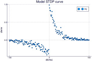
Functions and enable to be close to biological experiments [7]:
5.2 First applications of our results
In the simple case of (3) we get:
And
One weight free and 2 neurons:
In this example of one weight free and 2 neurons, we get a birth and death process with fixed, . We can find the explicit stationnary distribution of the weights in that case. From previous computations we have:
Hence, it is similar to a birth process on with 0 reflecting. In order to study the conditions for transience and recurrence, we use the following theorem which gather some results of the four first sections of [28] with its notations.
Theorem 5.1.
Suppose is a birth and death process on with birth rates for all and death rates for all and . Then [28] gives the following classification:
-
(a)
The process is ergodic if and only if and . In this case, there exists a unique invariant measure given by:
With
-
(b)
The process is null recurent if and only if and
-
(b)
The process is transient if and only if and
In order to apply this theorem to our example, we prove the following corollary.
Corollary 5.2.
Suppose assumptions of theorem 5.1 hold. Suppose in more that and converge respectively towards and when . Then is ergodic iff and transient if .
Proof.
Let prove only the ergodic case as the proof for the transient one is similar. Suppose that . Thus, for all , such that for all , and . Taking gives the result according to the d’Alembert’s ratio test. ∎
Remark 4.
The case is more complex as it will depend on the way and converge.
We come back to our example.
Proposition 5.3.
and are strictly positive and converge respectively to and when .
Proof.
First, and don’t depend on . Second, , and depend on only through . But so converges to solution of (50) with and . Concerning , we can fix and call . Computations of 78 show that for all , for all and is continuous as a positive bounded rational fraction. Hence, is continuous by composition. We conclude that and:
It is similar for .
∎
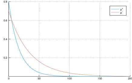
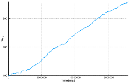
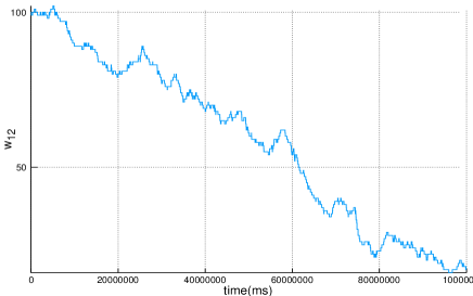
We then wonder when this condition holds and we did simulations with parameters in the range of biological ones. Practically, explosion of the weight reflects the fact that LTP wins over LTD. Some studies has tried to tackle question of the relationship between STDP curve parameters, and , and the balance of LTP and LTD. They showed that when the integral of the STDP window is enough biased toward depression the system is intrinsically stable [29, 30, 25]. In our case, we can find examples for which the "enough" is important. For instance with the following parameters, we get an explosion of when depression wins against potentiation:
We took . When is small enough () simulations agrees with analytical results. That is to say diverges when and doesn’t diverge when :
Remark 5.
We can even get divergence when for all
Example with 2 excitatory neurons
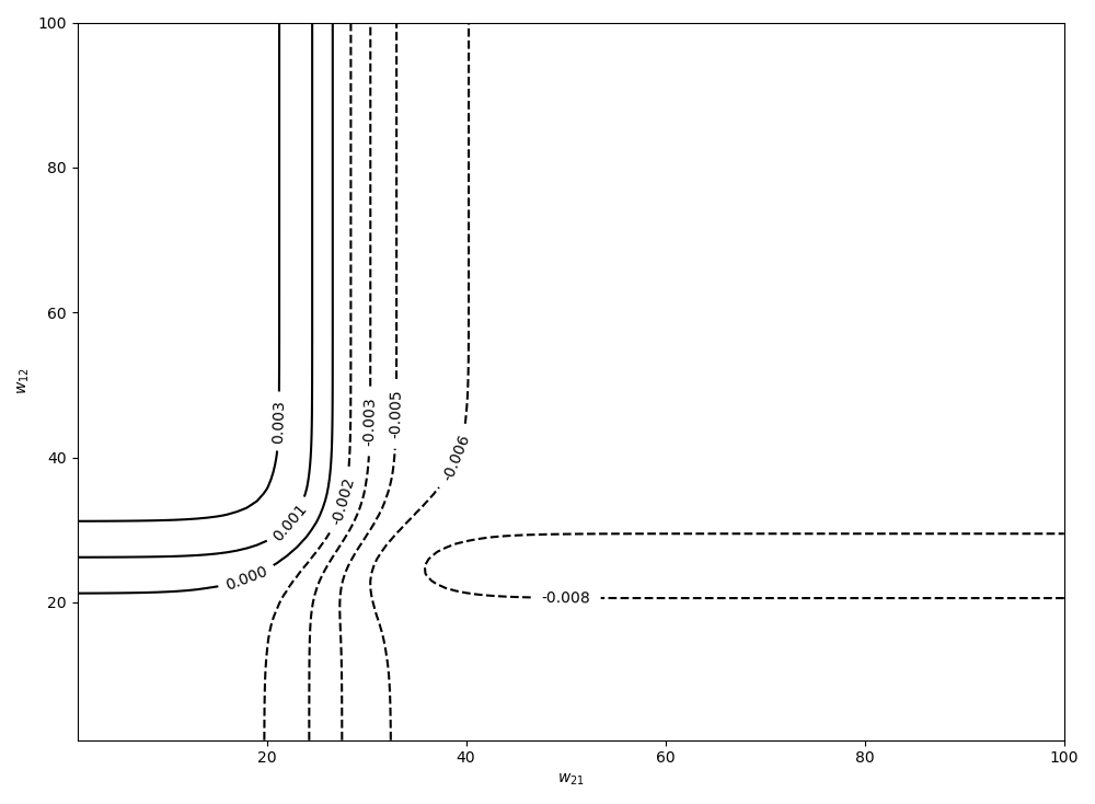
Let’s apply this result in a network of 2 excitatory neurons. First, we denote since the diagonal elements are null. We are interested in the sign of the limit of which is equivalent to (see 3), when , in order to use corollary 4.2 to study stability of weights. We first show this limit exists and then compute it to determine parameters for which we don’t have weights divergence.
In order to show the existence of the limit, we first recall that is only present in neurons’ rates. Thus, thanks to the sigmoid, these rates are bounded and when one of the components of goes to , rates in which it plays a role tends to the upper bound of the sigmoid, , since all neurons are excitatory ones. For instance:
Therefore, we can separate the space as following the intuition given by the graph of for instance:
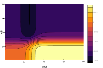
So the separation looks like this:
![[Uncaptioned image]](/html/1706.00364/assets/separate-space.png)
As showed in the appendix A, we can compute the Laplace transforms for fixed . If we introduce the dependence on , it will be in rate terms such as for example. As they are not numerous, we finish this kind of translation: , , and . So we can rewrite as a function of and . Therefore, when , on . The sup of becomes on and on . We conclude with
We can compute numerically this limit in function of and :
We note that we need a really small value of compared to the one of to satisfy the condition of positive recurrence. However, such a difference doesn’t seem to be needed in simulations. Indeed, we can have numerically positive recurrence for any parameters between 0 and 1.
Remark 6.
The condition for null recurrence given in [37] result in for all in our case. Condition for transience leads to the exact opposite of the one of corollary 4.2:
| (49) | ||||
It would be interesting to try to have a larger range of values of parameters for which we are in the null recurrence case, and we need another plasticity rule to do so (with the condition of [37]).
10 neurons:
When depression is really higher than potentiation, weights seem to converge to a stationary distribution and have such trajectories:
![[Uncaptioned image]](/html/1706.00364/assets/weight_traj.png)
![[Uncaptioned image]](/html/1706.00364/assets/density_weights.png)
However, initial weights can play an important role. With parameters and , we have no divergence in short time with low initial weights and selection of one weight from big initial ones, :
![[Uncaptioned image]](/html/1706.00364/assets/weight_sel.png)
The selected weight is different from one trajectory to another.
Remark 7.
We have chosen 10 neurons for plotting constraints. Thousands of them are easily simulated.
This kind of phenomenon is called winner take all dynamics in [33] where they prevent them using iSTDP. The reason to avoid them is that it prevents new assemblies to be formed.
6 Discussion
Mathematical results
Based on a well known neural network model, we added plasticity in order to get insight on the combined neurons - weights dynamics. We could analyse plasticity on the slow time scale of weights dynamics compared to the neurons ones, thus producing a simplified model. This latter gives the weights dynamics under the stationary distribution of the fast process and is a continuous time Markov jump process on the state space of weights with non homogeneous in space jump rates. Such processes are hard to deal with and current results are given in [37]. Moreover, even if we could prove existence and uniqueness of the invariant measure of the fast process, we were not able to express it explicitly. Thus, it is even harder to analyse the limit model. However, we can compute its Laplace transform in small networks, we didn’t try more than 2 but it should not be too hard for more. The problem will nevertheless become quickly harder as it consists in inverting a square matrix for a given and as soon as change, this computation need to be done again. Here, making use of bounds on jump rates of neurons, we are able to give conditions of stability, but we emphasize it is only sufficient ones. To know if we need additive terms, depending on weights for instance or just hard bounds, in order to avoid divergence in the context of biological parameters is still under study.
Simulation results
For small networks (2 neurons) and in the case of a STDP rule following the classical STDP curve [7], we computed Laplace transform of the stationary distribution. We then gave explicit expression of jump rates for the limit process which enabled us to study the weight dynamics more precisely. We even show that the divergence of weights is possible even when integral of the learning window is biased towards synaptic depression, even when depression curve is always stronger than depression ( for all ). Such a result is not intuitive and led us to find conditions on parameters for which such a divergence doesn’t occur. Simulations with more than two neurons showed the winner take all phenomenon takes place. A calibration of parameters is needed to test more characteristics of the model: how does it respond to high frequence, low frequence? Does it enable bidirectional connections?…
Limitations of our model and future work
We are aware our neuron model is far from the reality of neurons. It is really simple in order to make the study of plasticity easier. Some questions raise when we try to match it with biology. For instance, what does represents? Many things at the same time: the time one neuron will influence others, the time of a spike as it will not be able to spike again until the moment it comes back to the state 0. Neurons are generally described through their membrane potential which has no link to our model. Then, observations such as potential depolarisation is needed to lead to potentiation cannot be checked or modelled. Moreover, the way their rate of jump from 0 to 1 depends on weights is not really clear and needs to be clarify, maybe there is a need to add delay as it is done in other papers [32].
While STDP seems good to keep in memory stimuli, even spontaneously after such inputs [33], it needs to forget somehow. This seems not be the case in our model. Such a phenomenon is possible for instance under homeostatic mechanisms [45, 48, 49, 33]. STDP plays the role of additive synaptic scaling as when a weight increases, let say , then decreases. It is not a good thing according to [45], as they observed multiplicative synaptic scaling in their experiments. This is understandable as it is too specific and seems not sufficient. It is not useless if you think as information supported by is the exact opposite of the one supported by , it enables neurons " to win time ". So there is a need to add homeostasis to our model. Metaplasticity or plastic inhibitory (iSTDP) neurons are the most used. Indeed, we studied only a network of excitatory neurons. Adding non plastic inhibitory neurons will just decrease the minimum of firing rates of neurons. However, plastic inhibitory neurons could prevent from divergence of weights. Finally, is imposed but it could be interesting to use it as an homeostatic factor, decreasing the firing rate when it is to high and increasing it when it is weak.
Relation to previous work
Analysis using the separation of time scale between weights dynamics and the network one has been done in many other articles [29, 30, 11, 18, 16, 40, 32]. They modelled neurons as Poisson, except for [40], and derived a similar equation for weights on their slow time scale. This equation mainly depends on the cross correlation matrix which is not easy to handle with. They use Taylor expansion and Fourier transform to approximate it for their simulations. In our model, such a matrix is hidden in the invariant measure of the fast process. Concerning the stability of weights, a similar result was found in [30] where "a stable fixed point of the output rate is possible if the integral over the learning window is sufficiently negative." As, in their model, rates are linear in weights, stability of rates is equivalent to weights stability. Even if it is not a necessary condition, we could give an idea of how much negative the integral over the learning window needs to be in order to have stability.
Conclusion
We propose a new view on STDP models. In contrast with tiny deterministic jumps of weights, weights have some weak probability to make a "big" jump. Thus, instead of continuous, weights are discrete [2, 44]. Associated to the inter arrival time of spikes and the network state, we get a Markov process. We simplified it thanks to a separation of time scale and found simple conditions of positive recurrence. This work opens a new framework of study for plasticity which we hope it will give rise to more mathematical results on plasticity in the following.
Annexes
Appendix A Dimension 2 for uniqueness
After giving the generator in 2 dimensions, we then compute the equation satisfies by the Laplace transform of a given stationary distribution for .
Generator
Proposition A.1.
and :
Or in a shorter version:
Proof.
Let , then by definition exists. Let’s compute it. We know that each element has only two neighbors (in the sens it can only reach two different states). We note the rates to reach the neighbor v’. We do the computations for :
Then we obtain:
The same kind of computations gives us the same as in the proposition , and . In order to have the other inclusion, we take , then we compute for :
From previous computations, we see the jump terms will disappear because f is uniformly continuous, and the transport term will vanish as because
If t small enough.
Hence, exists. As we can do exactly the same computations for all , we deduce that . Thus, we have the equality wanted.
∎
We can see here the need to chose instead of for instance. Indeed, the uniform continuity enable us to conclude on the domain of B and on another hand it is the biggest subspace of on which the derivative is the generator of a -semigroup. If we had chosen , we see immediately the semigroup associated to our process will not map into itself. has no reason to vanish at . seems to be the space that suits. Moreover, thanks to the portmanteau lemma, the knowledge of the semigroup on characterizes the law of the process. We can then use the definition 3.10 to search the Laplace transforms of invariant measures.
Laplace transform
First, we show we can write any invariant measure of the process in the form where is the only invariant measure of the jump process and is a measure on . Then, we prove that if the process has at least one invariant measure of probability , then it is unique.
It is interesting to look at the form of invariant measures for the following. Indeed, as doesn’t depend on , we can study its dynamic and deduce a nice decomposition of the stationary distribution of .
Proposition A.2.
The jump process alone has a unique invariant probability measure . Moreover, , and it satisfies:
| (50) |
Proof.
Indeed, as each neuron is connected to each other, is irreducible. As its state space is finite, the process is also positive recurrent so has a unique invariant probability measure by theorem1.7.7 in [39].
Moreover, as each state is positive recurrent, .
The matrix is the matrix of transition rates (Q-matrix) of . With , and we have Q has in the proposition. As is invariant, it belongs to the kernel of Q, which is (50), Theorem 3.5.5 in [39].
∎
From this result, we deduce that . Therefore, we define as , . Hence, .
Now, we previously showed the process has at least one invariant probability measure on , let be one of them and let’s compute its Laplace transform to show the following proposition:
Proposition A.3.
Assume the process has at least one invariant measure of probability . Then it is unique.
Proof.
We will show that all invariant measure of probability has the same Laplace transform and as the later characterizes it, see for instance Theorem 4.3 in [26], there only exists one invariant measure of probability.
We can write as , with . To simplify computations, we will denote by be the vector of Laplace transforms of . So :
Just a remark,
As we want to compute the Laplace transform of which is in fact , let’s use the following test functions, with and :
By definition 3.10 of an invariant measure we get :
| (51) |
We then compute :
So with (51) and for instance:
After computations for all we get:
| (60) |
With:
As we have and .
Then we can get and evaluating (60) in and :
As , so:
And
Putting terms in in matrices marked we get:
| (69) |
With:
And
As a triangular superior matrix with diagonal elements strictly positive, is invertible. Moreover, and are invertible as diagonally dominant matrices whenever :
First line of (50) gives:
So :
For other lines we have :
We have similar results for which shows et are diagonally dominant matrices so they are invertible . Hence, if is an invariant measure for , :
By (69):
| (78) |
By (60)
We conclude using the fact the Laplace transform of a law determines it, so is unique. ∎
References
- [1] L. F. Abbott and S. B. Nelson. Synaptic plasticity: taming the beast. Nature neuroscience, 3:1178–1183, 2000.
- [2] D. J. Amit and S. Fusi. Learning in neural networks with material synapses. Neural Computation, 6(5):957–982, 1994.
- [3] P. A. Appleby and T. Elliott. Synaptic and temporal ensemble interpretation of spike-timing-dependent plasticity. Neural computation, 17(11):2316–2336, 2005.
- [4] P. A. Appleby and T. Elliott. Stable competitive dynamics emerge from multispike interactions in a stochastic model of spike-timing-dependent plasticity. Neural computation, 18(10):2414–2464, 2006.
- [5] M. Benayoun, J. D. Cowan, W. van Drongelen, and E. Wallace. Avalanches in a Stochastic Model of Spiking Neurons. PLoS Computational Biology, 6(7):e1000846, July 2010.
- [6] M. K. Benna and S. Fusi. Computational principles of synaptic memory consolidation. Nature Neuroscience, 19(12):1697–1706, Oct. 2016.
- [7] G.-q. Bi and M.-m. Poo. Synaptic modifications in cultured hippocampal neurons: dependence on spike timing, synaptic strength, and postsynaptic cell type. Journal of neuroscience, 18(24):10464–10472, 1998.
- [8] E. L. Bienenstock, L. N. Cooper, and P. W. Munro. Theory for the development of neuron selectivity: orientation specificity and binocular interaction in visual cortex. Technical report, DTIC Document, 1981.
- [9] P. C. Bressloff. Metastable states and quasicycles in a stochastic Wilson-Cowan model of neuronal population dynamics. Physical Review E, 82(5), Nov. 2010.
- [10] N. Brunel. Is cortical connectivity optimized for storing information? Nature Neuroscience, 19(5):749–755, Apr. 2016.
- [11] A. N. Burkitt, H. Meffin, and D. B. Grayden. Spike-timing-dependent plasticity: the relationship to rate-based learning for models with weight dynamics determined by a stable fixed point. Neural Computation, 16(5):885–940, 2004.
- [12] C. Clopath, L. Büsing, E. Vasilaki, and W. Gerstner. Connectivity reflects coding: A model of voltage-based spike-timing-dependent-plasticity with homeostasis. Nature, 2009.
- [13] M. H. Davis. Piecewise-deterministic Markov processes: A general class of non-diffusion stochastic models. Journal of the Royal Statistical Society. Series B (Methodological), pages 353–388, 1984.
- [14] M. H. A. Davis. Markov models and optimization. Monographs on statistics and applied probability. Chapman & Hall, London ; New York, 1st ed edition, 1993.
- [15] K. Fox and M. Stryker. Integrating Hebbian and homeostatic plasticity: introduction. Philosophical Transactions of the Royal Society B: Biological Sciences, 372(1715):20160413, Mar. 2017.
- [16] M. N. Galtier and G. Wainrib. A Biological Gradient Descent for Prediction Through a Combination of STDP and Homeostatic Plasticity. Neural Computation, 25(11):2815–2832, Nov. 2013.
- [17] W. Gerstner and W. M. Kistler. Spiking neuron models: single neurons, populations, plasticity. Cambridge University Press, Cambridge, U.K. ; New York, 2002.
- [18] M. Gilson, A. N. Burkitt, D. B. Grayden, D. A. Thomas, and J. L. van Hemmen. Emergence of network structure due to spike-timing-dependent plasticity in recurrent neuronal networks. I. Input selectivity–strengthening correlated input pathways. Biological Cybernetics, 101(2):81–102, Aug. 2009.
- [19] M. Gilson, A. N. Burkitt, D. B. Grayden, D. A. Thomas, and J. L. van Hemmen. Emergence of network structure due to spike-timing-dependent plasticity in recurrent neuronal networks V: self-organization schemes and weight dependence. Biological Cybernetics, 103(5):365–386, Nov. 2010.
- [20] M. Gilson, T. Fukai, and A. N. Burkitt. Spectral Analysis of Input Spike Trains by Spike-Timing-Dependent Plasticity. PLOS Computational Biology, 8(7):e1002584, 2012.
- [21] M. Graupner and N. Brunel. Calcium-based plasticity model explains sensitivity of synaptic changes to spike pattern, rate, and dendritic location. PNAS, 109(52):21551–21552, 2012.
- [22] M. Hairer. Convergence of Markov processes. lecture notes, 2010.
- [23] D. Hebb. The Organization of Behavior. Wiley & Sons. Wiley, New York, 1st ed edition, 1949.
- [24] E. M. Izhikevich. Dynamical systems in neuroscience: the geometry of excitability and bursting. Computational neuroscience. MIT Press, Cambridge, Mass, 2007. OCLC: ocm65400606.
- [25] E. M. Izhikevich and N. S. Desai. Relating stdp to bcm. Neural computation, 15(7):1511–1523, 2003.
- [26] O. Kallenberg. Foundations of modern probability. Springer Science & Business Media, 2006.
- [27] H.-W. Kang and T. G. Kurtz. Separation of time-scales and model reduction for stochastic reaction networks. The Annals of Applied Probability, 23(2):529–583, Apr. 2013.
- [28] S. Karlin and J. McGregor. The classification of birth and death processes. Transactions of the American Mathematical Society, 86(2):366–400, 1957.
- [29] R. Kempter, W. Gerstner, and J. L. Van Hemmen. Hebbian learning and spiking neurons. Physical Review E, 59(4):4498, 1999.
- [30] R. Kempter, W. Gerstner, and J. L. Van Hemmen. Intrinsic stabilization of output rates by spike-based Hebbian learning. Neural computation, 13(12):2709–2741, 2001.
- [31] T. G. Kurtz. Averaging for martingale problems and stochastic approximation. In Applied Stochastic Analysis, pages 186–209. Springer, 1992.
- [32] G. Lajoie, N. I. Krouchev, J. F. Kalaska, A. L. Fairhall, and E. E. Fetz. Correlation-based model of artificially induced plasticity in motor cortex by a bidirectional brain-computer interface. PLOS Computational Biology, 13(2):e1005343, 2017.
- [33] A. Litwin-Kumar and B. Doiron. Formation and maintenance of neuronal assemblies through synaptic plasticity. Nature communications, 5:5319, 2014.
- [34] H. Markram. A history of spike-timing-dependent plasticity. Frontiers in Synaptic Neuroscience, 3, 2011.
- [35] H. Markram, W. Gerstner, and P. J. Sjöström. Spike-Timing-Dependent Plasticity: A Comprehensive Overview. Frontiers in Synaptic Neuroscience, 4, 2012.
- [36] H. Markram, J. Lübke, M. Frotscher, and B. Sakmann. Regulation of synaptic efficacy by coincidence of postsynaptic aps and epsps. Science, 275(5297):213–215, 1997.
- [37] M. Menshikov, S. Popov, and A. Wade. Non-homogeneous Random Walks: Lyapunov Function Methods for Near-Critical Stochastic Systems, volume 209. Cambridge University Press, 2016.
- [38] A. Morrison, M. Diesmann, and W. Gerstner. Phenomenological models of synaptic plasticity based on spike timing. Biological Cybernetics, 98(6):459–478, June 2008.
- [39] J. R. Norris. Markov chains. Number 2. Cambridge university press, 1998.
- [40] G. K. Ocker, A. Litwin-Kumar, and B. Doiron. Self-organization of microcircuits in networks of spiking neurons with plastic synapses. PLoS Comput Biol, 11(8):e1004458, 2015.
- [41] D. H. O’Connor, G. M. Wittenberg, and S. S.-H. Wang. Graded bidirectional synaptic plasticity is composed of switch-like unitary events. Proceedings of the National Academy of Sciences of the United States of America, 102(27):9679–9684, 2005.
- [42] E. Pechersky, G. Via, and A. Yambartsev. Stochastic Ising model with plastic interactions. Statistics & Probability Letters, 123:100–106, Apr. 2017.
- [43] P. E. Protter. Stochastic Integration and Differential Equations: Version 2.1. Number 21 in Stochastic Modelling and Applied Probability. Springer, Berlin, 2. ed. , corr. 3rd pr edition, 2010. OCLC: 837782643.
- [44] C. Ribrault, K. Sekimoto, and A. Triller. From the stochasticity of molecular processes to the variability of synaptic transmission. Nature Reviews Neuroscience, 12(7):375–387, June 2011.
- [45] G. G. Turrigiano. The dialectic of Hebb and homeostasis. Philosophical Transactions of the Royal Society B: Biological Sciences, 372(1715):20160258, Mar. 2017.
- [46] R. L. Tweedie. Invariant Measures for Markov Chains with no Irreducibility Assumptions. Journal of Applied Probability, 25:275–285, 1988.
- [47] P. Yger and M. Gilson. Models of Metaplasticity: A Review of Concepts. Frontiers in Computational Neuroscience, 9, Nov. 2015.
- [48] F. Zenke, W. Gerstner, and S. Ganguli. The temporal paradox of Hebbian learning and homeostatic plasticity. Current Opinion in Neurobiology, 43:166–176, Apr. 2017.
- [49] F. Zenke, G. Hennequin, and W. Gerstner. Synaptic Plasticity in Neural Networks Needs Homeostasis with a Fast Rate Detector. PLoS Computational Biology, 9(11):e1003330, Nov. 2013.