Compacton solutions and (non)integrability of nonlinear evolutionary PDEs associated with a chain of prestressed granules

Abstract

We present the results of study of a nonlinear evolutionary PDE (more precisely, a one-parameter family of PDEs) associated with the chain of pre-stressed granules. The PDE in question supports solitary waves of compression and rarefaction (bright and dark compactons) and can be written in Hamiltonian form. We investigate inter alia integrability properties of this PDE and its generalized symmetries and conservation laws.

For the compacton solutions we perform a stability test followed by the numerical study. In particular, we simulate the temporal evolution of a single compacton, and the interactions of compacton pairs. The results of numerical simulations performed for our model are compared with the numerical evolution of corresponding Cauchy data for the discrete model of chain of pre-stressed elastic granules.

Keywords: chains of pre-stressed granules; compactons; integrable systems; symmetry integrability; symmetries; conservation laws; stability test; conserved quantities; Hamiltonian structures; numerical simulation

MSC 2010 35B36; 74J35; 74H15; 37K05; 37K10

1 Introduction

This paper deals with nonlinear evolutionary PDEs associated with dynamics of a one-dimensional chain of pre-stressed granules which arises in quite a number of applications. Since Nesterenko’s pioneering works [1, 2] propagation of pulses in such media has been a subject of a great number of experimental studies and numerical simulations, see [3, 4, 5, 6, 7, 8, 9, 10, 11, 12, 13] and references therein. We consider a nonlinear evolutionary PDE which is derived from the infinite system of ODEs describing the dynamics of one-dimensional chain of elastic bodies interacting with each other by means of a nonlinear force. The PDE in question is obtained through the passage to continuum limit followed by the formal multi-scale decomposition.

The PDE under study turns out to admit a Hamiltonian representation and possess localized traveling wave solutions manifesting some features of solitons. For this reason, it is of interest to investigate its complete integrability. We do this below along with the study of generalized symmetries and conservation laws. We show below that the compacton traveling wave (for traveling waves in general see e.g. [14, 15] and references therein) solutions satisfy the necessary condition for the extremum of a functional associated with the Hamiltonian. Using this we also perform a stability test followed by the numerical study of the compacton solutions. Somewhat surprisingly, numerical simulations show that even in a nonintegrable case the compacton solutions recover their shapes after the collisions, yet the dynamics of interaction slightly differs from that of KdV solitons. In this connection note that compactons, i.e. soliton-like solutions with compact support, see [1, 3, 16] and references therein, exist for a number of physically relevant models and possess several interesting features making them a subject of intense research, cf. e.g. [17, 18, 19, 20, 21, 22] and references therein.

The paper is organized as follows. In section 2 we introduce the continual analog of the granular pre-stressed media with the specific interaction of the adjacent blocks which allows for the description of both the waves of compression and rarefaction. In section 3 we present the Hamiltonian structure of the equation in question. In section 4 we study the conservation laws admitted by the said equation. In section 5 we perform the integrability test that singled out an exceptional integrable case, which is studied in more detail in section 6. In section 7 we show that the compacton traveling wave (TW) solutions that satisfy factorized equations also satisfy necessary conditions of extrema for the appropriate Lagrange functionals. Next we perform stability tests for compacton solutions based on the approach developed in [23, 24, 25], and show that both dark and bright compactons pass the stability test. The results of qualitative analysis are backed and partly supplemented by the numerical study performed in section  8. We also present the results of numerical simulation of the Cauchy problem for discrete chains and compare the results obtained with the analogous simulations performed for the continual analogue of these chains. The closing section 9 contains conclusions and discussion.

2 Evolutionary PDEs associated with the granular prestressed chains

Amazing features of the solitons associated with the celebrated Korteweg–de Vries (KdV) equation, as well as other completely integrable models [14], are often ascribed to the existence of higher symmetries and infinite sets of conservation laws, cf. e.g. [26, 27, 28]. However, there exist non-integrable equations possessing localized TW solutions with quite similar behavior. A well-known example of this is provided by the $K(m,n)$ equations [16]:

$$K(m,n):u_{t}+\left(u^{m}\right)_{x}+\left(u^{n}\right)_{xxx}=0,\qquad m\geq 2,\qquad n\geq 2.$$ (1)

The members of this hierarchy are not completely integrable at least for generic values of the parameters $m$, $n$, see [17, 20] and references therein, and yet possess compactly-supported TW solutions exhibiting solitonic features [16, 29].

The $K(m,n)$ family was introduced in the 1990s as a formal generalization of the KdV hierarchy without referring to its physical context. Earlier V.F. Nesterenko [1] considered the dynamics of a chain of preloaded granules described by the following ODE system:

$$\ddot{Q}_{k}(t)=F(Q_{k-1}-Q_{k})-F(Q_{k}-Q_{k+1}),\qquad k\in\left\{0,\pm 1,\pm 2\dots.\right\}$$ (2)

where $Q_{k}(t)$ is the displacement of the $k$th granule center-of-mass from its equilibrium position,

$$F(z)=Az^{n},\qquad n>1.$$ (3)

He has described for the first time the formation of localized wave patterns and evolution within this model [1, 2, 3]. In [1, 2, 5] he presented the nonlinear evolutionary PDEs being the quasi-continual limits of the discrete models; in this connection cf. also [30].

The transition to the continual model is achieved via the substitution

$$Q_{k}(t)=u(t,k\cdot a)\approx u(t,x),$$ (4)

where $a$ is the average distance between granules. Insert this formula, together with the substitutions

$$\begin{array}[]{rcl}Q_{k\pm 1}=u(t,x\pm a)&=&\exp(\pm aD_{x})u(t,x)\\ &=&\displaystyle\sum_{j=0}^{4}\frac{(\pm a)^{j}}{j!}\frac{\partial^{j}}{\partial x^{j}}u(t,x)+O\left(a^{5}\right),\end{array}$$ (5)

into (2), and observe that the term of lowest order in $a$ on the right-hand side of (2) is proportional to $a^{n+1}$. Now expanding the right-hand side of (2) divided by $a^{n+1}$ into the (formal) Taylor series and then dropping the terms of the order $O(a^{4})$ and higher in this expansion yields from (2) the equation

$$u_{tt}=-C\left\{\left(-u_{x}\right)^{n}+\beta\left(-u_{x}\right)^{\frac{n-1}{2}}\left[\left(-u_{x}\right)^{\frac{n+1}{2}}\right]_{xx}\right\}_{x},$$

where

$$C=Aa^{n+1},\qquad\beta=\frac{na^{2}}{6(n+1)}.$$

Differentiating the above equation with respect to $x$ and employing the new variable $S=\left(-u_{x}\right)$ corresponding to the strain field, one obtains the Nesterenko equation [5]:

$$S_{tt}=C\left\{S^{n}+\beta S^{\frac{n-1}{2}}\left[S^{\frac{n+1}{2}}\right]_{xx}\right\}_{xx}.$$ (6)

Eq. (6) was derived using only one small parameter corresponding to the long wave approximation. Thus it can describe the dynamics of “strongly preloaded media” with dynamic amplitude much smaller than the preload or the dynamics of “weakly preloaded media” when the dynamic amplitude in the wave is much larger than the preload or even when the preload is equal to zero, in which case the propagation of acoustic waves is impossible (the effect of “sonic vacuum” [2]). As it is shown in [5], equation (6) possesses a one-parameter family of compacton TW solutions describing the propagation of the waves of compression.

Unfortunately, the compacton solutions supported by (6) are unstable. This can be verified by a direct numerical calculation, substituting in the corresponding difference scheme as Cauchy data known compacton solutions.

A similar situation occurs in the case of the Boussinesq equation, obtained as a continuum limit of the Fermi–Pasta–Ulam system of coupled oscillators [14]. As is well known, the Boussinesq equation possesses unstable soliton-like solutions, and the KdV equation, supporting the stable uni-directional solitons, is extracted from the Boussinesq equation by means of the asymptotic multi-scale expansion [14], cf. also [31] and references therein.

In this connection it should be also noted that the instability caused by the short wavelengths can be removed using the regularization consisting in replacing the space derivatives of the force by mixed space and time derivatives. The regularized equation for the case of general power law is nothing but Eq. (1.110) from [5], and its counterpart for a general interaction law is Eq. (1.156) from [5].

It should be further noted that, at least for $n=3/2$, equation (6) has stationary compacton solutions which are close to the numerical solutions of the discrete Hertzian chain, see e.g. [8], and the numerical simulations and experiments strongly suggest that the latter solutions are stable. For example, such solutions are generated from various initial conditions on short distances from the disturbed end and propagate in experiments despite disturbances due to inevitable dissipation and violation of periodicity, see e.g. experimental results in [5].

Another interesting observation is that the conditions for existence of solitary waves in discrete chain [32] and in the continuum approximation, see Eq.(1.154) at p. 108 in [5], are identical and based on the sign of the second derivative of the force, see p. 113 in [5].

Our approach to finding a “proper” compacton-supporting equation is as follows. We start from the discrete system (2) in which the interaction force has the form

$$F(z)=Az^{n}+Bz.$$ (7)

In addition, we assume that $B=\gamma a^{n+3}$, where $|\gamma|=O(|A|)$.

The interaction law in (7) is a special case of general interaction law that results in long wave equation, Eq.(1.154) at p. 108 in [5] or its regularized counterpart, Eq.(1.156) in [5]. The stationary solutions of the said long wave equation are studied in [5], where, depending on the behavior of the second derivative of the interaction law, strongly nonlinear compression or rarefaction solitary waves are predicted.

In this connection also note that for small deformations the interaction law in (7) is a special case of the situation where the first derivative is nonzero and higher derivatives are zero except for the $n$-th order one which, in conjunction with the discussion in the preceding paragraph implies, cf. [5], in particular p.110–123, that the linear part of the interaction law is, to an extent, irrelevant for the study of qualitative behavior of stationary solutions.

Inserting (4), (5) into the formula (2) and assuming that the interaction is described by (7), we obtain, up to the terms of the order $O(a^{4})$ and higher in the expansion of the right-hand side of (2) divided by $a^{n+1}$, cf. the discussion after (5), the equation

$$u_{tt}=-C\left\{\left(-u_{x}\right)^{n}+\beta\left(-u_{x}\right)^{\frac{n-1}{2}}\left[\left(-u_{x}\right)^{\frac{n+1}{2}}\right]_{xx}\right\}_{x}-\gamma a^{n+3}\left(-u_{x}\right)_{x}.$$

Differentiating the above equation with respect to $x$ and introducing the new variable $S=\left(-u_{x}\right)$, we obtain the following equation:

$$S_{tt}=C\left\{S^{n}+\beta S^{\frac{n-1}{2}}\left[S^{\frac{n+1}{2}}\right]_{xx}\right\}_{xx}+\gamma a^{n+3}S_{xx}.$$ (8)

Now we use a series of scaling transformations. Employing the scaling $\tau=\sqrt{\gamma a^{n+3}}t$ enables us to rewrite the above equation in the form

$$S_{\tau\tau}=\frac{C}{\gamma a^{n+3}}\left\{S^{n}+\beta S^{\frac{n-1}{2}}\left[S^{\frac{n+1}{2}}\right]_{xx}\right\}_{xx}+S_{xx}.$$

Next, the transformation $\bar{T}=\frac{1}{2}a^{q}\tau$, $\xi=a^{p}(x-\tau)$, $S=a^{r}W$ is used. If, for example, we assign the following values to the parameters $q=1$, $p=-1$, $r=5/n,$ then the higher-order coefficient $O(a^{2})$ will be that of the second derivative with respect to $\bar{T}$. So, dropping the terms proportional to $O(a^{2})$, we obtain, after the integration with respect to $\xi$, the equation:

$$W_{\bar{T}}+\frac{A}{\gamma}\left\{W^{n}+\frac{n}{6(n+1)}W^{\frac{n-1}{2}}\left[W^{\frac{n+1}{2}}\right]_{\xi\xi}\right\}_{\xi}=0.$$

Performing the rescaling and returning to the initial notation

$$t=\frac{A}{\gamma}L\bar{T},\qquad x=L\xi,$$

where $L=\sqrt{\frac{6(n+1)}{n}}$, we finally obtain the sought-for equation

$$W_{T}+\left\{W^{n}+W^{\frac{n-1}{2}}\left[W^{\frac{n+1}{2}}\right]_{XX}\right\}_{X}=0,$$ (9)

to which we shall hereinafter refer as to the Nesterenko equation. Note that Eq.(9) appears in [19] (see also [22]) as a particular case of the $C_{1}(m,a+b)$ hierarchy introduced as a generalization of the set of $K(m,n)$ equations.

The description of waves of rarefaction in the case $n=2k$ requires the following modification of the interaction force:

$$F(z)=-Az^{2k}+Bz$$ (10)

(for $n=2k+1$ the formula (7) describes automatically both waves of compression and of rarefaction). Applying the above machinery to (2) with the interaction (10), we obtain, in the same notation, the equation

$$W_{T}-\left\{W^{n}+W^{\frac{n-1}{2}}\left[W^{\frac{n+1}{2}}\right]_{XX}\right\}_{X}=0,\quad n=2k.$$ (11)

Thus, the universal equation describing waves of compression and rarefaction for arbitrary $n\in\mathbb{N}$ can be written in the form

$$W_{T}+\left[\mathrm{sgn}(W)\right]^{n+1}\left\{W^{n}+W^{\frac{n-1}{2}}\left[W^{\frac{n+1}{2}}\right]_{XX}\right\}_{X}=0.$$ (12)

In closing note that equations (9), (11) and (12) are obtained by formal application of the multiscale decomposition method which cannot be substantiated in our case because of negativity of the index $p$, cf. [33] where this problem is discussed in a more general fashion. Further study of these equations is justified by the fact that they possess a set of compacton solutions possessing interesting dynamical features. As will be shown below, these solutions describe well enough propagation of short impulses in the chain of pre-stressed blocks.

3 Hamiltonian structure for the Nesterenko equation

Now return to (9) which we now write in the manifestly evolutionary form, that is,

$$W_{T}=-\left(W^{n}+W^{(n-1)/2}\left[W^{(n+1)/2}\right]_{XX}\right)_{X}$$ (13)

Note that for $n=-1$ this equation boils down to a quasilinear first-order equation $W_{T}=(W^{-1})_{X}$ which is obviously integrable, and for $n=1$ equation (13) becomes linear.

Equation (13) can be written (cf. [22]) as

$$W_{T}=D_{X}\delta\mathcal{H}_{\mathrm{Nest}}/\delta W\equiv F.$$ (14)

Thus, (14) is written in Hamiltonian form with the Hamiltonian $\mathcal{H}_{\mathrm{Nest}}$ and the Hamiltonian structure $\mathfrak{P}_{0}=D_{X}$.

This implies, in particular, that to any nontrivial local conserved density of (14) there corresponds a (generalized, but not necessarily genuinely generalized (see the definition below), and possibly trivial) symmetry of (14).

Here $\delta/\delta W$ is the variational derivative (see below for details) and $\mathcal{H}_{\mathrm{Nest}}=\displaystyle\int h_{\mathrm{Nest}}dX$ with the density

$$h_{\mathrm{Nest}}=\left\{\begin{array}[]{l}\displaystyle\left(\frac{1}{4}(n+1)W^{n-1}W_{X}^{2}-W^{n+1}/(n+1)\right)\quad\mbox{for $n\neq-1$},\\[14.22636pt] \displaystyle\ln|W|\quad\mbox{for $n=-1$.}\end{array}\right.$$ (15)

Here and below the integrals are understood in the sense of formal calculus of variations, see e.g. [28, 34]. Here we put, cf. [27, 28, 34], $W_{j}=\partial^{j}W/\partial X^{j}$, $j=1,2,\dots$, $W_{0}\equiv W$, and define [26, 27, 28, 34] the total derivatives

$$D_{X}=\displaystyle\frac{\partial}{\partial X}+\sum\limits_{j=0}^{\infty}W_{j+1}\displaystyle\frac{\partial}{\partial W_{j}},\quad D_{T}=\displaystyle\frac{\partial}{\partial T}+\sum\limits_{j=0}^{\infty}D_{X}^{j}(F)\displaystyle\frac{\partial}{\partial W_{j}}.$$ (16)

The variational derivative of a functional $\mathcal{F}=\displaystyle\int f(X,T,W,W_{1},\dots,W_{k})dX$ has the form

$$\frac{\delta\mathcal{F}}{\delta W}=\sum\limits_{j=0}^{\infty}(-D_{X})^{j}\left(\displaystyle\frac{\partial f}{\partial W_{j}}\right).$$ (17)

For any $f=f(X,T,W,\dots,W_{k})$ we also define, cf. e.g. [27, 28], its linearization

$$f_{*}=\sum\limits_{j=0}^{k}\displaystyle\frac{\partial f}{\partial W_{j}}D_{X}^{j}.$$

4 Conservation laws

Recall, cf. e.g. [26, 27, 28, 34, 35, 36, 37, 38] and references therein, that a local conservation law for (13) is, roughly speaking, a relation of the form

$$D_{T}(\rho)=D_{X}(\sigma),$$ (18)

where $\rho=\rho(X,T,W,W_{1},\dots,W_{r})$ and $\sigma=\sigma(X,T,W,W_{1},\dots,W_{s})$, which holds by virtue of (13). Here $\rho$ and $\sigma$ are called a (conserved) density and the flux of our conservation law.

Also recall, cf. e.g. [36], that a conservation law (18) is called nontrivial if there exists no function $\zeta(X,T,W,W_{1},\dots,W_{q})$ such that $\rho=D_{X}\zeta$, i.e., $\rho\not\in\mathrm{Im}D_{X}$.

It is well known, see e.g. [28, 34], that a necessary and sufficient condition for a function $f=f(X,T,W,W_{1},\dots,W_{r})$ to not belong to the image of $D_{X}$ is $E_{W}f\neq 0$, where $E_{W}$ is the Euler operator

$$E_{W}=\sum\limits_{j=0}^{\infty}(-D_{X})^{j}\circ\displaystyle\frac{\partial}{\partial W_{j}}.$$

Hence $\rho$ is a conserved density for (13) if and only if $E_{W}D_{T}(\rho)=0$, and this density is nontrivial if and only if $E_{W}\rho\neq 0$.

It is readily checked that we have the following

Proposition 1.

For any $n$ equation (13) admits the following three conserved densities:

$$\rho_{0}=W,\quad\rho_{1}=W^{2}/2,\quad\rho_{2}=h_{\mathrm{Nest}}.$$ (19)

For $n=0$ we have an extra density

$$\rho_{3}=X^{2}WW_{X}-TW_{X}^{2}/W.$$ (20)

Moreover, for $n\neq 0,1,-1,-2$ (resp. for $n=0$) the densities (19) (resp. (19 and (20)) exhaust, modulo the addition of trivial ones, the linearly independent conserved densities of order up to five, i.e., of the form $\rho=\rho(X,T,W,W_{X},\dots,W_{XXXXX})$.

It is very likely that for $n\neq 1,-1,-2$ no local conserved densities of order greater than five (of course, again modulo trivial ones) exist at all in view of nonintegrability of (13) for $n\neq 1,-1,-2$ as discussed below.

Recall that $\rho_{2}$ is the density of the Hamiltonian $\mathcal{H}_{\mathrm{Nest}}$ for (13) with respect to the Hamiltonian structure $\mathfrak{P}_{0}=D_{X}$. To the functional $\mathcal{C}=\displaystyle\int WdX$ there corresponds a trivial symmetry, i.e., a symmetry with zero characteristic, as $D_{X}\delta\mathcal{C}/\delta W=0$, so $\mathcal{C}$ is a Casimir functional for $\mathfrak{P}_{0}$. To the functional $\mathcal{P}=\frac{1}{2}\displaystyle\int W^{2}dX$ there corresponds a symmetry with the characteristic $W_{X}=D_{X}\delta\mathcal{P}/\delta W$, that is, $X$-translation, and to $\mathcal{H}_{\mathrm{Nest}}$ there corresponds a symmetry with the characteristic equal to the r.h.s. $F$ of (14), i.e., the time translation symmetry.

For $n=0$ to the conserved functional $\mathcal{H}_{3}=\displaystyle\int\rho_{3}dX$ there corresponds a scaling symmetry with the characteristic $4TF+2XW_{X}+2W=D_{X}\delta\mathcal{H}_{3}/\delta W$. Again, it is very likely that $\rho_{i}$, $i=0,\dots,3$, are the only local conserved densities (modulo trivial ones) for (13) with $n=0$ in view of nonintegrability of this special case of (13).

5 Integrability

Integrable equations of the form (14) with the Hamiltonian of general form $\mathcal{H}=\displaystyle\int dXh(W,W_{X})$ where the density $h=h(W,W_{X})$ is such that $\partial^{2}h/\partial W_{X}^{2}\neq 0$ were classified (modulo point transformations leaving $T$ invariant) in [39]. Note that in [27, 39] and references therein integrability of an evolution equation

$$W_{T}=K(X,W,W_{X},\dots,\partial^{k}W/\partial X^{k})$$ (21)

with $k\geq 2$ means existence of an infinite hierarchy of generalized symmetries of increasing orders which do not depend explicitly on $T$. In order to avoid ambiguity we shall, following the common usage, refer below to this kind of integrability as to the symmetry integrability.

Recall, cf. e.g. [26, 27, 28, 34], that a generalized symmetry of order $r$ for (21) is a function $G=G(X,T,W,W_{1},\dots,\allowbreak W_{r})$ such that $\partial G/\partial W_{r}\neq 0$ and

$$D_{T}(G)=K_{*}(G),$$ (22)

where now $D_{T}=\displaystyle\frac{\partial}{\partial T}+\sum\limits_{j=0}^{\infty}D_{X}^{j}(K)\displaystyle\frac{\partial}{\partial W_{j}}$.

Such a symmetry $G$ is known as genuinely generalized if it cannot be written in the form $G=c(T)K+b(X,T,W,W_{X})$ for some functions $b$ and $c$, that is, it is not equivalent to a point or contact symmetry. As far as point symmetries of the equations studied in the present paper, and, more broadly, of $\mathcal{C}_{1}(m,a,b)$ equations (see e.g. [19, 22]), cf. e.g. [40] and references therein.

Thus, symmetry integrability of (21) means existence of an infinite hierarchy of generalized symmetries of the form $G_{i}(X,W,W_{1},\dots,W_{r_{i}})$ of increasing orders $r_{i}$.

Now turn to comparison of the density $h_{\mathrm{Nest}}$ of our Hamiltonian and the densities $h$ found in [39] for which the equation $W_{T}=D_{X}(\delta\mathcal{H}/\delta W)$ with the general Hamiltonian $\mathcal{H}=\displaystyle\int h(W,W_{X})dX$ is symmetry integrable.

Proposition 2.

The only symmetry integrable case of (13) which is genuinely nonlinear and genuinely of third order is that of $n=-2$.

Proof. It is not difficult to observe (cf. e.g. [41]) that using point transformations leaving $t$ invariant the density $h_{\mathrm{Nest}}$ of our Hamiltonian for $n\neq-1$ can, if at all, only be transformed into just one case from [39], namely, equation (2.1) in [39], that is,

$$h=W_{X}^{2}/(2f^{3})-P/f,$$ (23)

where $f=c_{0}+c_{1}W+c_{2}W^{2}$, $P=\sum\limits_{i=0}^{4}d_{i}W^{i}$, and $c_{i}$ and $d_{i}$ are arbitrary constants.

Moreover, it is clear that in our case $f$ should actually be a monomial: $f=cW^{\alpha}$, $\alpha=0,1,2$.

Upon comparing the coefficients at $W_{X}^{2}$ in (23) and (15) modulo an obvious rescaling of $W$, we see that all values of $n$ for which (13) could be integrable should satisfy $n-1=0,-3,-6$. The case of $n=1$ is trivially integrable, as then (13) is just a linear equation, so we are left with two possibilities $n=-2$ and $n=-5$ corresponding to $\alpha=1$ and $\alpha=2$.

Now upon inspecting the remaining terms in $h_{\mathrm{Nest}}$ and in (23) we readily conclude that the polynomial $P$ should also reduce to a single monomial: $P=dW^{\beta}$, where $\beta=0,1,2,3,4$, so we have a system $n-1=-3\alpha$ and $n+1=\beta-\alpha$, where $\alpha=1,2$ and $\beta=0,1,2,3,4$. An obvious corollary of this system is $-3\alpha+2=\beta-\alpha$, whence $\beta=2(1-\alpha)$. However, $\beta\geq 0$ by assumption, so the case of $n=-5$, when $\alpha=2$ and we should have $\beta=-2$, is not integrable.

Thus, the only integrable case of (13) which is genuinely nonlinear and genuinely of third order is that of $n=-2$, and the result follows. $\Box$.

Recall that for $n=-1$ equation (13) degenerates and becomes a first order quasilinear equation whose general solution can be found, see above, and for $n=1$ equation (13) is just linear.

In fact, the result of Proposition 2 can be further strengthened so that absence of any generalized symmetries, rather than just those that do not depend explicitly on $T$, can be established.

To this end consider, following [27], the so-called canonical density $\rho_{-1}=(\partial F/\partial W_{XXX})^{-1/3}$. It is readily checked that $E_{W}D_{T}(\rho_{-1})\neq 0$ for $n\neq-1,-2,-5,1$. Hence for $n\neq-1,-2,-5,1$ we have $D_{T}(\rho_{-1})\not\in\mathrm{Im}\ D_{X}$, and thus $\rho_{-1}$ is not a density of a local conservation law for (13).

In turn, by virtue of the results from [42] this immediately implies

Proposition 3.

Equation (13) for $n\neq 1,-1,-2,-5$ has no generalized symmetries of order greater than three.

In other words, Proposition 3 means that for $n\neq 1,-1,-2,-5$ any solution $G=G(X,T,W,W_{1},\dots,W_{r})$ of the equation

$$D_{T}(G)=F_{*}(G),$$ (24)

where $D_{T}$ and $F$ are given in (16) and (14), in fact depends at most on $X,T,W,W_{X},W_{XX},W_{XXX}$.

This implies that (13) for $n\neq-1,-2,-5,1$ admits no genuinely generalized symmetries, and hence (13) for $n\neq-1,-2,-5,1$ is unlikely to be integrable in any reasonable sense, cf.  [27].

Leaving aside the degenerate cases of $n=\pm 1$, turn to the remaining two special cases: $n=-2$ and $n=-5$. We believe that using the technique similar to that of [43] (cf. also [20, 44]) it can be shown that in the case of $n=-5$ equation (13) admits no genuinely generalized symmetries, including those with explicit dependence on $T$ and not just the time-independent ones whose nonexistence follows from the above comparison of (15) with (23), so we are left with just one integrable case of $n=-2$ which we discuss below.

6 Nesterenko equation for $n=-2$: integrability and beyond

The following result is readily checked by straightforward computation:

Proposition 4.

For $n=-2$ equation (13) has a Lax pair of the form

$$\psi_{XX}=(1+W^{2}\lambda)\psi,\quad\psi_{T}=\frac{2}{W^{3}}\psi_{XXX}-\frac{3W_{X}}{W^{4}}\psi_{XX}+\frac{2}{W^{3}}\psi_{X}-\frac{3W_{X}}{W^{4}}\psi$$ (25)

and admits a recursion operator

$$\begin{array}[]{rcl}\mathfrak{R}&=&\displaystyle\frac{1}{W^{2}}D_{X}^{2}-\frac{3W_{X}}{W^{3}}D_{X}+\frac{(4W^{2}+6W_{X}^{2}-3W_{XX})}{W^{4}}\\[14.22636pt] &&-2\left(W^{-2}+W^{-3/2}\left[W^{-1/2}\right]_{XX}\right)_{X}D_{X}^{-1}\end{array}$$ (26)

The recursion operator (26) can be found e.g. using the technique from [45] (cf. also [46]). Also note that upon passing to a new dependent variable equal to a square of $W$ the first equation of (25) can be identified with a special case of the eigenvalue problem related to the extended Harry Dym systems, see e.g. [47] and references therein.

Equation (13) for $n=-2$ also admits a second local Hamiltonian operator $\mathfrak{P}_{1}=\mathfrak{R}\circ D_{x}$, that is,

$$\begin{array}[]{rcl}\mathfrak{P}_{1}&=&\displaystyle\frac{1}{W^{2}}D_{X}^{3}-\frac{3W_{X}}{W^{3}}D_{X}^{2}+\frac{(4W^{2}+6W_{X}^{2}-3W_{XX})}{W^{4}}D_{X}\\[14.22636pt] &&-2\left(W^{-2}+W^{-3/2}\left[W^{-1/2}\right]_{XX}\right)_{X}\end{array}$$

which is compatible with $\mathfrak{P}_{0}=D_{X}$, so the recursion operator $\mathfrak{R}$ is hereditary and equation (13) for $n=-2$ can be written, in addition to (14), in the second Hamiltonian form as

$$W_{T}=\mathfrak{P}_{0}(\delta\tilde{h}/\delta W),$$ (27)

where $\tilde{h}=W/2$.

Thus, we have the following

Proposition 5.

Equation (13) for $n=-2$ is an integrable bihamiltonian system with two local Hamiltonian operators $\mathfrak{P}_{0}$ and $\mathfrak{P}_{1}$ and two local Hamiltonian representations (14) and (27).

Using general theory of bihamiltonian systems (see e.g. [28, Ch. 7] and [48]), we also readily obtain

Corollary 1.

Equation (13) for $n=-2$ possesses an infinite hierarchy of commuting generalized symmetries of the form $\mathfrak{R}^{k}W_{X}$, $k=0,1,2,\dots$ and an infinite hierarchy of local conservation laws whose densities $h_{j}$ are generated recursively through the relations

$$\mathfrak{P}_{0}(\delta h_{j+1}/\delta W)=\mathfrak{P}_{1}(\delta h_{j}/\delta W),$$

where $j=0,1,2,\dots$ and $h_{0}=W/2$, and of associated integrals of motion $\mathcal{H}_{j}=\int h_{j}dX$ in involution with respect to the two Poisson brackets associated with $\mathfrak{P}_{0}$ and $\mathfrak{P}_{1}$.

The fact that the generalized symmetries $\mathfrak{R}^{k}W_{X}$ and the conserved densities $h_{k}$ for $k=0,1,2,\dots$ do not involve any nonlocal terms can be established using the results of [49] or [50] (cf. also [46]).

As we have already pointed out above, up to a suitable rescaling of $T$ and obvious change of notation equation (14) for $n=-2$ is a special case of equation (2.1c) in [39], and hence can be transformed into a special case of the well-known $S$-integrable Calogero–Degasperis–Fokas [51, 52] equation in the manner described therein.

Namely, pass first to the potential form of (14) with $n=-2$,

$$V_{T}=-\frac{V_{XXX}}{2V_{X}^{3}}+\frac{3V_{XX}^{2}}{4V_{X}^{4}}+\frac{1}{V_{X}^{2}},$$

related to (13) through the differential substitution $W=V_{X}$.

The subsequent hodograph transformation interchanging $X$ and $V$ turns the above equation into a constant separant equation

$$V_{T}=-\frac{V_{XXX}}{2}+\frac{3V_{X}V_{XX}}{2V}-\frac{3V_{X}(4+V_{X}^{2})}{4V^{2}},$$

or, upon a suitable rescaling of $T$,

$$V_{T}=V_{XXX}-\frac{3V_{X}V_{XX}}{V}+\frac{3V_{X}(4+V_{X}^{2})}{V^{2}}.$$ (28)

Finally, putting $V=\exp(U/2)$ turns (28) into a special case of the Calogero–Degasperis–Fokas [51, 52] equation, viz.,

$$U_{T}=U_{XXX}-\frac{1}{8}U_{X}^{3}+6U_{X}\exp(-U).$$ (29)

7 Compacton solutions and stability tests

Consider the pair of equations (9), (11), which can be represented by the single expression

$$W_{T}+\epsilon\left\{W^{n}+W^{\frac{n-1}{2}}\left[W^{\frac{n+1}{2}}\right]_{XX}\right\}_{X}=0,\quad\epsilon=\pm 1.$$ (30)

As we are interested in the traveling wave (TW) solutions $W=W(z)\equiv W(X-cT)$, it is convenient to pass to the TW coordinates $T\to T$, $X\to z=X-cT$. This change of variables yields from (30) the equation

$$W_{T}-cW_{z}+\epsilon\left\{W^{n}+W^{\frac{n-1}{2}}\left[W^{\frac{n+1}{2}}\right]_{zz}\right\}_{z}=0.$$ (31)

It is easy to check that equation (31) admits a Hamiltonian formulation

$$W_{T}=D_{z}{\delta\left(\epsilon\mathcal{H}_{\mathrm{Nest}}+c\mathcal{P}\right)}/{\delta W},$$ (32)

where now

$$\mathcal{H}_{\mathrm{Nest}}=\int h_{\mathrm{Nest}}dz,\qquad\mathcal{P}=\int\frac{1}{2}W^{2}dz,$$

and

$$h_{\mathrm{Nest}}=\left\{\begin{array}[]{l}\displaystyle\left(\frac{1}{4}(n+1)W^{n-1}W_{z}^{2}-W^{n+1}/(n+1)\right)\quad\mbox{for $n\neq-1$},\\[14.22636pt] \displaystyle\ln|W|\quad\mbox{for $n=-1$.}\end{array}\right.$$

The above formulation up to the coefficient $\epsilon$ follows directly from the Hamiltonian form (cf. (14)) of equation (9) after the change of coordinates. Recall that both functionals $\mathcal{H}_{\mathrm{Nest}}$ and $\mathcal{P}$ are conserved in time.

Now consider the following functions:

$$W_{c}^{\epsilon}(z)=\epsilon W_{c}(z)=\begin{cases}\epsilon M\cos^{\gamma}\left(Kz\right),&\mathrm{if}\quad|Kz|<\frac{\pi}{2},\\ 0&\quad\mathrm{otherwise},\\ \end{cases}$$ (33)

where $\epsilon=\pm 1$,

$$M=\left[\frac{c(n+1)}{2}\right]^{\frac{1}{n-1}},\qquad K=\frac{n-1}{n+1},\qquad\gamma=\frac{2}{n-1}.$$

It is readily checked that we have the following

Proposition 6.

If $n=2k+1$, $k\in\mathbb{N}$, then the functions $W_{c}^{\pm}(z)$ are weak solutions to the equation

$$\delta\left(\mathcal{H}_{\mathrm{Nest}}+c\mathcal{P}\right)/\delta W|_{W=W_{c}^{\pm}}=0.$$ (34)

If $n=2k$, $k\in\mathbb{N}$, then the functions $W_{c}^{\pm 1}(z)$ are weak solutions to the equation

$$\delta\left(\pm\mathcal{H}_{\mathrm{Nest}}+c\mathcal{P}\right)/\delta W|_{W=W_{c}^{\pm 1}}=0.$$ (35)

So, the TW solutions (33) are the critical points of either the Lagrange functional $\Lambda=\mathcal{H}_{\mathrm{Nest}}+\beta\mathcal{P}$ (the case of $n=2k+1$) or $\Lambda^{\epsilon}=\epsilon\mathcal{H}_{\mathrm{Nest}}+\beta\mathcal{P}$ (the case of $n=2k$) with the common Lagrange multiplier $\beta=c$. As is well known, necessary and sufficient condition for $\Lambda$ (resp. $\Lambda^{\epsilon}$) to attain the minimum on the compacton solutions can be stated in terms of the positivity of the second variation of the corresponding functional, which, in turn, guarantees the orbital stability of the TW solution [53]. Here we do not touch upon the problem of strict estimating of the signs of the second variations. We follow instead the approach suggested in [23, 24, 25], which enables us to test the possibility of appearance of the local minimum on selected sets of perturbations of TW solutions.

Consider the following family of perturbations

$$W_{c}^{\epsilon}(z)\rightarrow\lambda^{\alpha}W_{c}^{\epsilon}(\lambda z).$$ (36)

Upon choosing $\alpha=1/2$ we obtain

$$\mathcal{P}[\lambda]=\frac{1}{2}\int_{-\pi/2}^{\pi/2}{\left[\lambda^{\frac{1}{2}}W_{c}^{\epsilon}(\lambda z)\right]^{2}dz}=\mathcal{P}[1].$$ (37)

Thus, for this choice $\mathcal{P}[\lambda]$ keeps its unperturbed value. By imposing this condition we reject “fake” perturbations associated with the translational symmetry $T_{\delta}\left[W_{c}^{\epsilon}(z)\right]=W_{c}^{\epsilon}(z+\delta)$. Indeed, since equations (34), (35) are invariant under the shift $z\to z+\delta$, $T_{\delta}W_{c}^{\epsilon}(z)$ belongs to the set of solutions as well, while formally the transformation $W_{c}^{\epsilon}(z)\rightarrow W_{c}^{\epsilon}(z+\delta)$ can be treated as a perturbation. In order to exclude the perturbations of this sort, the orthogonality condition is imposed. Introducing the representation for the perturbed solution

$$W_{c}^{\epsilon}(z)[\lambda]=W_{c}^{\epsilon}(z)+v(z,\lambda),$$

and using the condition (37), we find

$$0=\mathcal{P}[\lambda]-\mathcal{P}[1]=\int_{-\pi/(2K)}^{\pi/(2K)}W_{c}^{\epsilon}(z)v(z,\lambda)dz+O\left(||v(z,\lambda)||^{2}\right),$$

so if $\mathcal{P}$ is independent of $\lambda$, then, up to $O\left(||v(z,\lambda)||^{2}\right)$ the perturbation created by the scaling transformation is orthogonal to the TW solution.

For $\alpha=1/2$ and $n\in\mathbb{N}$, we arrive at the following functions to be tested:

$$\Lambda^{\nu}[\lambda]=(\nu\mathcal{H}_{\mathrm{Nest}}+c\mathcal{P})[\lambda]=\nu\left\{\lambda^{\frac{n+3}{2}}I_{n}^{\epsilon}-\lambda^{\frac{n-1}{2}}J_{n}^{\epsilon}\right\}+c\mathcal{P},$$ (38)

where

$$I_{n}^{\epsilon}=\frac{n+1}{4}\int_{-\pi/(2K)}^{\pi/(2K)}\left[W_{c}^{\epsilon}\right]^{n-1}\left[\left(W_{c}^{\epsilon}\right)_{z}\right]^{2}dz,\qquad J_{n}^{\epsilon}=\frac{1}{n+1}\int_{-\pi/(2K)}^{\pi/(2K)}\left[W_{c}^{\epsilon}\right]^{n+1}dz,$$

$$\nu=\epsilon^{n+1}=\begin{cases}+1&\mathrm{if}\quad n=2k+1,\\ \quad\epsilon&\mathrm{if}\quad n=2k.\\ \end{cases}$$

If the functional $\Lambda^{\nu}=\nu\mathcal{H}_{\mathrm{Nest}}+c\mathcal{P}$ attains the extremal value on the compacton solution, then the function $\Lambda^{\nu}[\lambda]$ has the corresponding extremum in the point $\lambda=1$. The verification of this property is employed as a test.

A necessary condition for the extremum $\frac{d}{d\lambda}\Lambda^{\nu}[\lambda]\Bigl{|}_{\lambda=1}=0$ gives us the equality

$$I_{n}^{\epsilon}=\frac{n-1}{n+3}J_{n}^{\epsilon}.$$ (39)

Using (39), we obtain the estimate

$$\frac{d^{2}}{d\lambda^{2}}\Lambda^{\nu}[\lambda]\Bigl{|}_{\lambda=1}=\nu(n-1)J_{n}^{\epsilon}=\frac{n-1}{n+1}\epsilon^{2(n+1)}\int\left[W_{c}^{\epsilon}\right]^{n+1}(z)dz>0,$$

which is valid for both $n=2k+1$ and $n=2k$. Thus, the generalized solutions (33) pass the test for stability, and we can state the following

Conjecture. For $n>1$ weak solutions (33) provide minima of the functional $\Lambda^{\nu}$.

Further information about the properties of the compacton solutions is provided by the numerical simulations discussed below.

8 Numerical simulations for dynamics of compactons

The dynamics of solitary waves is studied by means of direct numerical simulation based on the finite-difference scheme.

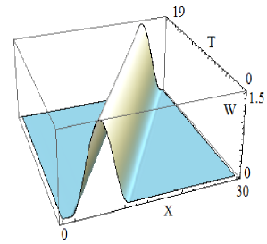
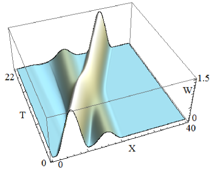
a)                                                      b)

Figure 1: Numerical evolution of a single compacton solution of Eq. (40) characterized by the velocity $c=1$ (a) and a pair of compacton solutions characterized by the velocities $c=1$ and $c=1/4$ (b), respectively.

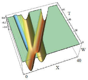
Figure 2: Numerical evolution of a pair of dark compactons characterized by the velocities $c=1$ and $c=1/4$, respectively.

To derive a finite-difference scheme, say, for the model equation (9), we modify the scheme presented in [29]. In agreement with the methodology proposed in that paper we introduce the artificial viscosity by adding the term $\varepsilon W_{4x}$, where $\varepsilon$ is a small parameter. Thus, instead of (9) we have for the case of $n=3$ the following equation:

$$W_{t}+\left\{W^{3}\right\}_{x}+\left\{W\left[W^{2}\right]_{xx}\right\}_{x}+\varepsilon W_{4x}=0.$$ (40)

Let us approximate the spatial derivatives as follows:

$$\begin{split}\frac{1}{120}(\dot{W}_{j-2}+26\dot{W}_{j-1}+66\dot{W}_{j}+26\dot{W}_{j+1}+\dot{W}_{j+2})+\\ +\frac{1}{24h}(-W_{j-2}^{3}-10W_{j-1}^{3}+10W_{j+1}^{3}+W_{j+2}^{3})+\\ +\frac{1}{24h}(-L_{j-2}-10L_{j-1}+10L_{j+1}+L_{j+2})+\\ +\varepsilon\frac{1}{h^{4}}(W_{j-2}-4W_{j-1}+6W_{j}-4W_{j+1}+W_{j+2})=0,\end{split}$$ (41)

where $L_{j}=W_{j}\frac{W_{j-2}^{2}-2W_{j}^{2}+W_{j+2}^{2}}{h^{2}}$ .

To integrate the system (41) in time, we use the midpoint method. Then the quantities $W_{j}$ and $\dot{W}_{j}$ are represented in the form

$$W_{j}\rightarrow\frac{W_{j}^{n+1}+W_{j}^{n}}{2},\dot{W}_{j}\rightarrow\frac{W_{j}^{n+1}-W_{j}^{n}}{\tau}.$$

The resulting nonlinear algebraic system with respect to $W_{j}^{n+1}$ can be solved by iterative methods.

We test the scheme (41) by considering the movement of a single compacton. Assume that the model parameters $c=1$ and the scheme parameters $N=600$, $h=30/N$, $\tau=0.01$, $\varepsilon=10^{-3}$ are fixed. The application of the scheme (41) gives us fig. 1a.

The starting profile providing the initial condition for the numerical scheme is chosen according to (33) where $n=3$, $c_{1}=1$ and $c_{2}=1/4$, namely,

$$W_{1,2}=\Bigl{\{}\begin{array}[]{l}\epsilon\sqrt{2c_{1,2}}\cos\left((z-z_{1,2})/2\right)\mbox{if}\left|(z-z_{1,2})/2\right|<\pi/2,\\ 0\ \mbox{otherwise}\end{array}$$

where $z_{1}=5$, $z_{2}=13$, and $\epsilon=+1$ for fig. 1 while $\epsilon=-1$ for fig. 2 (note that $W_{i}$ corresponds to $i$-th figure).

To study the interaction of two bright compactons, we combine the compacton having the velocity $c=1$ with the slow one characterized by the velocity $c=1/4$ and being shifted to the right at the initial moment of time. The result of modelling is presented at fig. 1b. The interaction of two dark compactons has similar properties and is depicted at fig. 2.

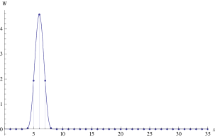
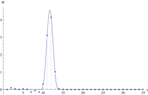
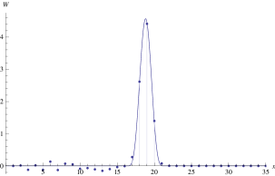
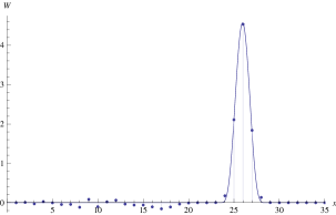
Figure 3: Evolution of the initial perturbation in the granular media (marked with dots) on the background of the corresponding evolution of the compacton (marked with solid lines) obtained at the following values of the parameters: $n=3/2$, $c=1.425$, $A=0.25,$ $B=0.3.$ Upper row: left: $t=0;$ right: $t=4$; lower row: left: $t=9$; right: $t=14$

As we have already mentioned at the end of Section 2, there is no way of selecting the scales in the model equations (9), (11) and (12), so the scaling decomposition employed there is rather formal. Nevertheless, it leads to interesting equations possessing localized solutions with solitonic features.

Now we are going to compare the evolution of the compacton solutions with corresponding solutions of the finite (but long enough) discrete system. Since the average distance $a$ between adjacent blocks does not play the role of a small parameter anymore, we assume from now on that it is equal to one. With this assumption in mind, we can write equation (12) in the initial variables $t,x$ as follows:

$$W_{t}+Q\left[\mathrm{sgn}(W)\right]^{n+1}\left\{W^{n}+\hat{\beta}W^{\frac{n-1}{2}}\left[W^{\frac{n+1}{2}}\right]_{xx}\right\}_{x}=0,$$ (42)

where

$$Q=\frac{A}{\gamma},\qquad\hat{\beta}=\frac{n}{6(n+1)}.$$

It is easy to verify that equation (42) possesses the following compacton solutions:

$$W_{c}^{\epsilon}(z)=\epsilon W_{c}(z)=\begin{cases}\epsilon\tilde{M}\cos^{\gamma}{\left(\tilde{B}z\right)},&\mbox{ if }|\tilde{B}z|<\frac{\pi}{2},\\ 0&\mbox{ otherwise},\\ \end{cases}$$ (43)

where $\epsilon=\pm 1,$ $z=x-ct,$

$$\tilde{M}=\left[\frac{c(n+1)}{2Q}\right]^{\frac{1}{n-1}},\qquad\tilde{B}=\frac{n-1}{(n+1)\sqrt{\beta}},\qquad\gamma=\frac{2}{n-1}.$$

We introduce the functions $R_{k}=Q_{k-1}-Q_{k}$ being the discrete analogs to the strain field $W(t,x)$. These functions are assumed to satisfy the system

$$\begin{array}[]{rcl}\ddot{R}_{1}(t)&=&0,\\ \ddot{R}_{k}(t)&=&A\left[R_{k-1}|R_{k-1}|^{n-1}-2R_{k}|R_{k}|^{n-1}+R_{k+1}|R_{k+1}|^{n-1}\right]\\[5.69054pt] &&+\gamma\left[R_{k-1}|R_{k-1}|^{n-1}-2R_{k}|R_{k}|^{n-1}+R_{k+1}|R_{k+1}|^{n-1}\right],\\[5.69054pt] k&=&2,\dots,m-1,\\ \ddot{R}_{m}(t)&=&0\end{array}$$ (44)

We solve this system with the following initial conditions induced by the compacton solution (43) in the respective nodes:

$$R_{k}(0)=\begin{cases}\epsilon\tilde{M}\cos^{\gamma}[\tilde{B}k-I]&\mbox{if}\ |\tilde{B}k-I|<\pi/2\\ 0&\mbox{otherwise},\end{cases}$$ (45)

$$\dot{R}_{k}(0)=\begin{cases}\epsilon\tilde{M}c\gamma\tilde{B}\cos^{\gamma-1}[\tilde{B}k-I]\sin[\tilde{B}k-I]&\mbox{if }|\tilde{B}k-I|<\pi/2\\ 0&\mbox{ otherwise},\end{cases}$$ (46)

$$R_{1}(0)=\dot{R}_{1}(0)=R_{m}(0)=\dot{R}_{m}(0)=0,$$ (47)

where $I$ is a constant phase, $k=2,3,\dots,m-1$. Note that $A$ and $\gamma$ appear in equation (42) in the form of the ratio $Q=A/\gamma$, whereas in the system (44) they appear as independent parameters. Therefore, one should not expect a one-to-one correspondence between the solutions of the discrete and continuous problems for arbitrary values of the parameters. The numerical experiments confirm this hypothesis by showing that synchronous evolution of the same compacton perturbation within two models can be observed for a unique value of the velocity $c=c_{0}$. This value depends strongly on the parameter $\gamma$ and depends on the parameter $A$ in a much weaker fashion. It has been observed that at $c<c_{0}$ the discrete compacton moves quicker than its continuous analogue while at $c>c_{0}$ the opposite effect occurs. The result of comparison for a single compacton is shown at fig. 3. One can see that at the chosen values of the parameters the main perturbations move synchronously and do not change their form. However, in the tail part of the discrete analogue small nonvanishing oscillations appear after a while.

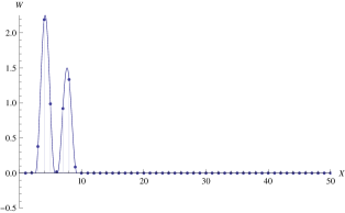
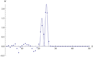
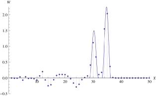
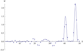
Figure 4: Evolution of two initially separated compacton perturbation in the granular media (marked with dots) on the background of the corresponding compacton solutions of the continual model (marked with solid lines), obtained at the following values of the parameters: $n=2$, $c_{1}=1.5$, $c_{2}=1.0$, $A=B=1.$ Upper row: left: $t=0$; right: $t=12$; lower row: left: $t=18.25$; right: $t=26$

Since for every value of the parameter $\gamma$ there is a unique value of the wave pack velocity for which the discrete and continuous compacton perturbations move synchronously, one should not expect that the collision of compactons within these two models will proceed in the same way for any set of values of parameters. However, collision processes display not much of qualitative differences for the discrete pulses which interact elastically like their continuous analogues. This is illustrated on fig. 4 showing the evolution of two initially separated discrete compactons. For convenience, the continuous compactons which coincide with the right-hand side of the initial data (45) at $t=0$ (the leftmost graph in the first row) are also shown in this figure. Continuous curves shown on the following graphs are obtained by appropriate translations. They are presented in order to emphasize the quasi-elastic nature of interaction of the discrete pulses.

9 Conclusions and discussion

In the present paper we have studied compacton solutions supported by the nonlinear evolutionary PDEs. The equations we considered, (9), (11), and (12), are obtained from the dynamical system (2) describing one-dimensional chain of prestressed elastic bodies. Equation (8) obtained in [5] from this model without resorting to the method of multi-scaled decomposition possesses the compacton solutions which fail the stability test. Numerical simulations show that the compacton solutions supported by equation (8) are destroyed in a very short time.

In contrast with the above, equations (9) (resp. (11)), which are obtained using formal multiscale decomposition, possess families of bright (resp. dark) compacton solutions which appear to be stable. This is backed both by the stability test and the results of the numerical simulations.

As we have shown in Sections 3–5, for generic values of the parameter $n$ equation (9) does not possess an infinite set of higher symmetries or other signs of complete integrability such as infinite hierarchies of conservation laws. Nevertheless the compacton solutions to this equation possess some features which are characteristic for “genuine” soliton solutions. In this connection it would be interesting to compare the traveling wave solutions for the distinguished case $n=-2$ with any other equation of the family (9) with negative $n$. Qualitative analysis of the factorized equations describing the TW solutions shows that there are no compacton solutions for the models with the negative $n$, but nevertheless all of them seem to possess periodic solutions resembling peakons. It would be interesting to find out whether there is any difference in the qualitative behavior of periodic solutions of the only integrable case ($n=-2$) in comparison with the periodic TW solutions supported by the model characterized by other values $n<0$. Perhaps the differences will be manifested in the stability properties as this is the case with the soliton solutions supported by the family of the KdV-type equations.

A characteristic feature of equations (9), (11) related to the decomposition we used is that they describe processes with “long” temporal and “short” spatial scales. Hence it is rather questionable whether these equations can adequately describe a localized pulse propagation in discrete media in the situation when the distance between the adjacent particles is comparable to the compacton width $\Delta x$. In fact, making the “reverse” transformations $X\rightarrow\xi\rightarrow x$ we get the following formula for the width of the compacton solution (33) in the initial coordinate system:

$$\Delta x=\pi a\sqrt{\frac{n(n+1)}{6(n-1)^{2}}};$$

this is nothing but equation (1.130) from [5]. For $n=3/2$, corresponding to the Hertzian force between spherical particles, we get $\Delta x\approx 4.96a$. It is then interesting to notice that the same results for the particles with the spherical geometry were obtained in the course of numerical simulations, and experimental studies [1, 3, 2, 54, 55]. We wish to stress that results of our analysis as well as the main conclusions are in agreement with the earlier publications by other authors. In particular, P. Rosenau notes, when considering the general models of dense chains [19], that the natural separation of scales leading to an unidirectional PDE of first order in time does not exist.

References

- [1] V.F. Nesterenko, Propagation of nonlinear compression pulses in granular media, J. Appl. Mech. Techn. Phys. 24 (1983), 733–743.
- [2] V.F. Nesterenko, Solitary waves in discrete media with anomalous compressibility and similar to “sonic vacuum”, Journal de Physique 4 (1994), C8-729–C8-734.
- [3] A.N. Lazaridi and V.F. Nesterenko, Observation of a new type of solitary waves in a one-dimensional granular medium, J. Appl. Mech. Techn. Phys., 26 (1985), 405–408.
- [4] C. Coste, E. Falcon and S. Fauve, Solitary waves in a chain of beads under Hertz contact, Phys. Rev. E 56 (1997), 6104–6117.
- [5] V.F. Nesterenko, Dynamics of Heterogeneous Materials, Springer-Verlag, New York, 2001.
- [6] C. Daraio, V.F. Nesterenko, E.B. Herbold, and S. Jin, Energy trapping and shock disintegration in a composite granular medium, Phys. Rev. Lett. 96 (2006), 058002.
- [7] E. Herbold and V.F. Nesterenko, Shock wave structure in strongly nonlinear lattice with viscous dissipation, Phys. Rev. E 75 (2007), 021304.
- [8] K. Ahnert and A. Pikovsky, Compactons and chaos in strongly nonlinear lattices, Phys. Rev. E 79 (2009), 026209.
- [9] G. Iooss, G. James, Localized waves in nonlinear oscillator chains, Chaos 15 (2005), no. 1, 015113, 15 pp.
- [10] G. James, Periodic travelling waves and compactons in granular chains, J. Nonlinear Sci. 22 (2012), no. 5, 813–848.
- [11] J. Yang, G. Silvestero, D. Khatri, L. De Nardo and Ch. Daraio, Interaction of highly nonlinear solitary waves with linear elastic media, Phys. Rev. E 83 (2011), 046606.
- [12] V.A. Vladimirov and S.I. Skurativskyi, Solitary waves in one-dimensional pre-stressed lattice and its continual analog, in: Dynamical systems. Mechatronics and life sciences, ed. by J. Awrejcewicz et al., Łódź, Politechnika Łódzka, 2015, 531–542, arXiv:1512.06125v1.
- [13] V.A. Vladimirov and S.I. Skurativskyi, On the spectral stability of soliton-like solutions to a non-local hydrodynamic-type model, arXiv:1807.08494.
- [14] R.K. Dodd, J.C. Eilbeck, J.D. Gibbon and H.C. Morris, Solitons and Nonlinear Wave Equations, Academic Press: London, 1984.
- [15] C. Valls, Algebraic traveling waves for the generalized Newell-Whitehead-Segel equation, Nonlinear Anal. Real World Appl. 36 (2017), 249–266.
- [16] P. Rosenau and J. Hyman, Compactons: solitons with finite wavelength, Phys. Rev. Lett. 70 (1993), 564–567.
- [17] P. Rosenau, On solitons, compactons, and Lagrange maps, Phys. Lett. A 211 (1996), no. 5, 265–275.
- [18] M. Destrade, G. Saccomandi, Solitary and compactlike shear waves in the bulk of solids, Phys. Rev. E 73 (2006), 065604(R), arXiv:nlin/0601021
- [19] P. Rosenau, On a model equation of traveling and stationary compactons, Phys. Lett. A 356 (2006), 44–50.
- [20] J. Vodová, A complete list of conservation laws for non-integrable compacton equations of type, Nonlinearity 26 (2013), 757–762, arXiv:1206.4401
- [21] E.N.M. Cirillo, N. Ianiro, G. Sciarra, Compacton formation under Allen-Cahn dynamics. Proc. R. Soc. A 472 (2016), no. 2188, 20150852, 15 pp.
- [22] A. Zilburg, P. Rosenau, On Hamiltonian formulations of the equations, Phys. Lett. A 381 (2017), 1557–1562.
- [23] G.H. Derrick, Comments on nonlinear wave equations as models for elementary particles, J. Math. Phys. 5 (1964), pp. 1252–1254.
- [24] E.A. Kuznetsov, A.M. Rubenchik and V.E. Zakharov, Soliton stability in plasmas and hydrodynamics, Phys. Rep. 142 (1986), 103–165.
- [25] V.I. Karpman, Stabilization of soliton instabilities by higher order dispersion: KdV-type equations, Phys. Lett. A 210 (1996), 77–84.
- [26] N.H. Ibragimov, Transformation groups applied to mathematical physics, Reidel, Boston, 1985.
- [27] A.B. Shabat, A.V. Mikhailov, Symmetries – Test of Integrability, in Important developments in soliton theory, Springer, Berlin etc., 1993, 355–374.
- [28] P.J. Olver, Applications of Lie groups to differential equations, 2nd ed., Springer, New York, 1993.
- [29] J. De Frutos, M. A. Lopez-Marcos and J. M. Sanz-Serna, A finite-difference scheme for the compacton equation, J. Comput. Phys. 120 (1995), 248–252.
- [30] V.F. Nesterenko, Waves in strongly nonlinear discrete systems, Phil. Trans. Roy. Soc. 376 (2018), no. 2127, 20170130.
- [31] G.I. Burde, A. Sergyeyev, Ordering of two small parameters in the shallow water wave problem, J. Phys. A: Math. Theor. 46 (2013), no. 7, article 075501, arXiv:1301.6672
- [32] G. Friesecke and J.A.D. Wattis, Existence theorem for solitary waves on lattices, Comm. Math. Phys. 161 (1994), no. 2, 391–418.
- [33] P. Rosenau, Hamilton dynamics of dense chains and lattices: or how to correct the continuum, Phys. Lett. A 31 (2003), 39–52.
- [34] I. Dorfman, Dirac structures and integrability of nonlinear evolution equations, John Wiley & Sons, Ltd., Chichester, 1993.
- [35] R.O. Popovych, A. Bihlo, Inverse problem on conservation laws, arXiv:1705.03547
- [36] R.O. Popovych, A. Sergyeyev, Conservation laws and normal forms of evolution equations, Phys. Lett. A 374 (2010), no. 22, 2210–2217, arXiv:1003.1648
- [37] A. Sergyeyev, New integrable (3+1)-dimensional systems and contact geometry, Lett. Math. Phys. 108 (2018), no. 2, 359–376, arXiv:1401.2122
- [38] D. Catalano Ferraioli, L.A. de Oliveira Silva, Nontrivial 1-parameter families of zero-curvature representations obtained via symmetry actions, J. Geom. Phys. 94 (2015), 185–198.
- [39] A.G. Meshkov, V.V. Sokolov, Integrable evolution Hamiltonian equations of the third order with the Hamiltonian operator , J. Geom. Phys. 85 (2014), 245–251.
- [40] M.S. Bruzón, M.L. Gandarias, M. Torrisi, R. Tracinà, On some applications of transformation groups to a class of nonlinear dispersive equations, Nonlinear Anal. Real World Appl. 13 (2012), no. 3, 1139–1151.
- [41] O.O. Vaneeva, R.O. Popovych and C. Sophocleous, Equivalence transformations in the study of integrability, Phys. Scr. 89 (2014) 038003, 9 p., arXiv:1308.5126 [nlin.SI]
- [42] A. Sergyeyev, On time-dependent symmetries and formal symmetries of evolution equations, in Symmetry and perturbation theory (Rome, 1998), G. Gaeta (ed.), 303–308, World Scientific, Singapore, 1999, arXiv:solv-int/9902002.
- [43] A. Sergyeyev, R. Vitolo, Symmetries and conservation laws for the Karczewska–Rozmej–Rutkowski–Infeld equation, Nonlinear Analysis: Real World Appl. 32 (2016), 1–9, arXiv:1511.03975
- [44] J. Vodová-Jahnová, On symmetries and conservation laws of the Majda–Biello system, Nonlinear Analysis: Real World Applications 22 (2015), 148–154, arXiv:1405.7858
- [45] M. Marvan, A. Sergyeyev, Recursion operator for the stationary Nizhnik–Veselov–Novikov equation, J. Phys. A: Math. Gen. 36 (2003), no. 5, L87–L92, arXiv:nlin/0210028
- [46] A. Sergyeyev, A Simple Construction of Recursion Operators for Multidimensional Dispersionless Integrable Systems, J. Math. Analysis Appl. 454 (2017), no. 2, 468–480, arXiv:1501.01955
- [47] M. Marvan, M.V. Pavlov, A new class of solutions for the multi-component extended Harry Dym equation, Wave Motion 74 (2017), 151–158.
- [48] P.J. Olver, Bi-Hamiltonian systems, in Ordinary and partial differential equations (Dundee, 1986), 176–193, Longman Sci. Tech., Harlow, 1987.
- [49] J.A. Sanders and J.P. Wang, On recursion operators, Physica D 149 (2001), 1–10.
- [50] A. Sergyeyev, Why nonlocal recursion operators produce local symmetries: new results and applications, J. Phys. A: Math. Theor. 38 (2005), no. 15, 3397–3407, arXiv:nlin/0410049.
- [51] F. Calogero and A. Degasperis, Reduction technique for matrix nonlinear evolution equations solvable by the spectral transform, J. Math. Phys. 22 (1981), 23–31.
- [52] A.S. Fokas, A symmetry approach to exactly solvable evolution equations, J. Math. Phys. 21 (1980), 1318–1325.
- [53] T. Kapitula and K. Promislow, Spectral and Dynamical Stability of Nonlinear Waves, Springer-Verlag: New York, 2013.
- [54] V.F. Nesterenko, A.N. Lazaridi and E.B. Sibiryakov, The decay of soliton at the contact of two “acoustic vacuums”, J. Appl. Mech. Techn. Phys. 36 (1995), 166–168.
- [55] D.B. Vengrovich, private communication.