Anomalous mass dimensions and Schwinger-Dyson equations boundary condition
Abstract
Theories with large mass anomalous dimensions () have been extensively studied because of their deep consequences for models where the scalar bosons are composite. Large values may appear when a non-Abelian gauge theory has a large number of fermions or is affected by four-fermion interactions. In this note we provide a simple explanation how can be directly read out from the IR and UV boundary conditions derived from the gap equation, and verify that moderate values appear when the theory possess a large number of fermions, but large values are obtained only when four-fermion interactions are added to the theory. We also verify how the critical line separating the different chiral phases emerge from these conditions.
pacs:
12.38.-t, 12.40.-y, 12.60.-iThe GeV resonance discovered at the LHC atlas has many of the characteristics expected for the Standard Model (SM) Higgs boson. If this particle is a composite or an elementary scalar boson is still an open question. Many models have considered the possibility of a light composite Higgs based on effective Higgs potentials as reviewed in Ref.h1 . The possibility that the Higgs boson is a composite state instead of an elementary one is more akin to the phenomenon of spontaneous symmetry breaking that originated from the Ginzburg-Landau Lagrangian, which can be derived from the microscopic BCS theory of superconductivity describing the electron-hole interaction.
The possibility of spontaneous symmetry breaking promoted by a composite scalar boson formed by new fermions has been discussed with the use of many models, the technicolor (TC) being the most popular one tc1 . However the phenomenology of these models depend crucially on these new fermions (or technifermions) self-energy. In the early models this self-energy was considered to be given by the standard operator product expansion (OPE) result politzer :
where is the TC condensate of order of a few hundred GeV, i.e. the order of the SM vacuum expectation value (vev). Unfortunately this behavior does lead to models with incompatibilities with the experimental data. A possible way out of this dilemma was proposed by Holdom holdom , remembering that the self-energy behaves as
| (1) |
where is the characteristic TC scale and the mass anomalous dimension associated to the fermionic condensate. As can be verified from Eq.(1) a large anomalous dimension leads to a hard asymptotic self-energy and may solve the many problems of the SM symmetry breaking promoted by composite bosons.
The work of Ref.holdom started the search for theories that could present a large mass anomalous dimension, leading to fermionic self-energies decreasing slowly with the momenta, and consequently to more realistic models of dynamical symmetry breaking (dsb). It is interesting to note that a hard asymptotic self-energy is even able to generate a scalar composite lighter than the scale of the SM vev us1 ; us2 . Models proposing such large anomalous dimensions were reviewed in Ref.yamawaki , and theories with large anomalous dimensions () are quite desirable for technicolor phenomenology sannino . Studies of these anomalous dimensions in many different non-Abelian models have been performed through analytical methods and lattice simulations as can be seen in Ref.g1 ; g2 ; g3 ; g4 ; g5 ; g6 ; g7 and references therein. The importance of these studies is not only related to the dsb model building but also to the knowledge of the different phases of non-Abelian gauge theories.
Early work with Schwinger-Dyson equations (SDE) in the case verified that and is not strongly affected by high order corrections g1 . Models with a slowly running coupling, i.e. near a non-trivial fixed point, in non-Abelian gauge theories started to be studied in Refs.apel ; ap4 ; ap5 and seems to enhance the values. In the Ref.apel the fixed point was obtained from the two-loop function for a theory with fermions in the fundamental representation. One analysis of this problem in the case of other groups and fermionic representations can be seen in Ref.sn2 . Large mass anomalous dimensions seems also to appear naturally in what is now known as gauged Nambu-Jona-Lasinio models, as shown in the works of Refs.yama1 ; yama2 ; mira2 ; yama3 ; mira3 ; yama4 . In these last type of models two coupling constants enter into action: the gauge coupling () and the 4-fermion one (), and there is a critical line described by a combination of these couplings where the chiral symmetry is broken. At this critical line the dynamical fermion mass behaves as a slowly decreasing function with the momentumtakeuchi ; kondo , and not much different from what is expected in a theory with bare masses.
Limits on can also be derived in specific models. An upper bound comes out from unitarity of conformal field theories g2 . Conformal bootstrap methods applied to symmetric conformal field theories suggest for g3 and for g4 . An enormous effort has been pursued by different groups performing lattice simulations to reveal values in with many flavors g5 ; g6 ; g7 . Some works may present different reflecting different approaches to determine this quantity. As one example we can quote the lattice simulation of Ref.g7 where the anomalous dimension for with was found to be relatively small, while a SDE approach taking into account four-fermion interactions produce a larger anomalous dimension for the same model us3 . However this fact may not be a surprise, but just may indicates that four-fermion interactions are necessarily responsible for large values.
In this note we were moved by the idea of showing in a simple way how the mass anomalous dimensions vary in different models, and will discuss how the boundary conditions of the anharmonic oscillator representation of the gap equation are directly related with the mass anomalous dimensions. We discuss how such boundary conditions (and ) are affected by inclusion of effects as a large number of fermions (leading to what is called walking theory), or by the inclusion of four-fermion interactions. We argue that the anomalous dimension can be read out directly from the boundary conditions, which is a simple result although we are not aware that this fact was stated before. We also recover the existence of the critical line, and verify how the mass anomalous dimensions may vary with the different boundary conditions after considering the numerical solution of the fermionic gap equation in the anharmonic oscillator representation. Lastly, we verify that without four-fermion interactions the existence of a large anomalous dimension is not compelling, whereas the opposite is true for a large range of coupling constants.
The fermionic SDE in Landau gauge for a gauge theory, with fermions in the fundamental representation, can be written as Richard ; georgi ; us4
| (2) |
where is the dynamical fermion mass, is the Casimir operator for fermions in the fundamental representation and is the running coupling constant. In order to simplify the analysis, we will assume the walking limit of this equation where is constant, in addition we also consider the set of new variables
| (3) |
With these new variables, after considering the chiral limit , Eq.(2) takes the following form
| (4) |
where , and . It is then possible to transform this integral equation into a differential one, which assumes the form
| (5) |
This representation for the gap equation in the walking regime was first obtained by Cohen and Georgi in Ref.georgi and corresponds to the equation of a unit mass subjected to the anharmonic potential
which is quadratic with a logarithmic correction due to the gauge theory. In the limit of small and large the potential is approximately harmonic, and in these limits the criticallity condition of Eq.(5) can be analyzed, making analogy with the critical behavior shown by a damped harmonic oscillator subjected to the boundary conditions in the infrared (IR)[] and ultraviolet (UV)[] regionsRichard ; georgi
| (6) |
The solution of the corresponding linearized equation [Eq.(5)] for is described by
| (7) |
where is the mass anomalous dimension of the quark condensate , , and .
Eq.(5) is described by a damped harmonic oscillator in the limit of small , which corresponds to the known behavior of the gap equation solution in the asymptotic region, , obtained for . According to Ref.georgi precisely in this case OPE provides an interpretation of the parameters appearing in the asymptotic solution of the gap equation. Moreover, dynamical chiral symmetry breaking does not occur for , on the other hand it is possible to investigate the critical behavior of this gap equation when with the following transformation georgi
| (8) |
With the new coordinate shown in Eq.(8) we can verify the following relation between and
| (9) |
Now the differential equation satisfied by takes the formgeorgi
| (10) |
and the boundary conditions for in the infrared (IR)[] and ultraviolet (UV)[] regions can be obtained from Eq.(9), leading to
| (11) |
The boundary conditions in the coordinate reflect the expected behavior of the dynamical fermion mass generated by the condensate in the infrared (IR)[] and ultraviolet (UV)[] limits. As observed by Cohen and Georgi: “chiral symmetry breaking resides not in the solutions to the gap equation, but in the boundary conditions” georgi . For example, if we include the asymptotic freedom behavior into the gap equation, i.e. the running charge , in the (UV) limit we have , and leads to
In the case of a large number of fermions (a walking theory) , where , we have and in this case
These examples illustrate as the boundary conditions, in the coordinate, are affected by the inclusion of effects like a large number of fermions (walking), or any interaction that modifies the behavior of the fermionic condensate . Looking at Eq.(11) it is still an open problem to find a viable phenomenological model where we may have a large in the perturbative Banks and Zaks scenario BZ . As we shall discuss in the following, the inclusion of four-fermion interactions will modify the boundary conditions presented in Eq.(11) in the (UV) region, and the new conditions will show clearly the possibility of a large range of values depending on the behavior of the new coupling constants.
Eq.(4) can be also represented by
| (12) |
where we identify
and if we include a four-fermion interaction we have a new contribution to the gap equation
| (13) |
with . The incorporation of the four-fermion interaction produces the following change in the boundary condition for in the ultraviolet region
| (14) |
Considering Eq.(9) the new boundary condition for the coordinate in the ultraviolet region becomes
| (15) |
The four-fermion interaction becomes relevant in the (UV) region when and the condition that determines the critical line for the gap equation [Eq.(10)], when , corresponds to in such a way that the boundary condition given by Eq.(15) leads to
| (16) |
where . Therefore, from Eq.(16), when we can determine the critical line which separates the symmetric and asymmetric chiral phases of a model with relevant four-fermion interaction; and this critical line is given by
| (17) |
Usually the critical line is determined from the asymptotic expansion of the hypergeometric function associated to the solution of the gap equation for , Eq.(2), after replacing this result into the ultraviolet boundary condition, giving the well known result yama1 ; yama2 ; mira2 ; yama3 ; mira3 ; yama4
| (18) |
For the purpose of comparison we show in Fig.(1) the behavior of the critical line obtained from the above equations
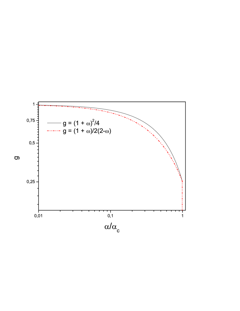
We emphasize that in our case we do not use the knowledge about the asymptotic expression assumed by , as usually performed to obtain Eq. (18). The determination of the critical line in our approach is only due to the modifications in the form assumed by the boundary condition as , due to the presence of an additional four-fermion interaction and the fact that the criticallity condition in this case is given by . Therefore in Figure 1 the two critical lines do not exhibit exactly the same behavior, on the other hand, in the extremes delimited by the (IR) and (UV) conditions this line accurately reflect the behavior of how the mass anomalous dimension of the fermionic condensate is modified by the inclusion of new interactions.
As we mentioned earlier, our intention was to verify how the mass anomalous dimensions may vary with the different boundary conditions after the inclusion of effects like the four-fermion interactions, therefore assuming the result described by Eq.(15), it is possible verify that for
| (19) |
so that when the four-fermion interactions becomes relevant and in this case . Thus, in order to verify how is modified by changes in the boundary conditions, we will consider the dynamical behavior of
| (20) |
and compute the numerical solution of the fermionic gap equation in the anharmonic oscillator representation, Eq.(10) for , with the different set of UV boundary conditions indicated by , where
| (21) |
and stands for OPE, walking (Walk) and four-fermion interaction (4F), with the limits , and (see Eqs.(11) and (19)). In the Fig.(2) we show the behavior of Eq.(20) for this set of different (UV) boundary conditions
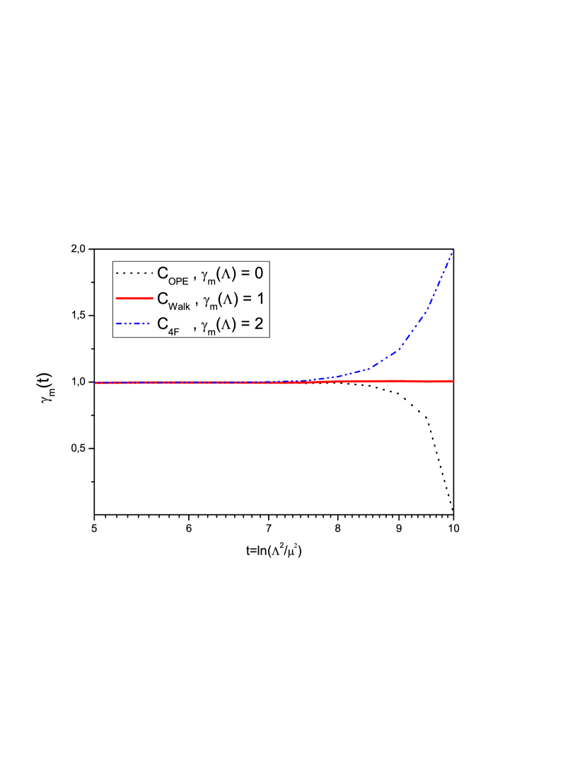
As mentioned at the beginning of this note there are many determinations of the mass anomalous dimension of models. Considering the different values obtained in the literature, despite the different methods to obtain this quantity, it is interesting to have a simple explanation of the origin of these values. In this note we discussed how the boundary conditions of SDE in the anharmonic oscillator representation are directly related with the mass anomalous dimensions, and how such conditions are affected by inclusion of effects like a large number of fermions or by inclusion of four-fermion interactions.
The fact that the introduction of four-fermion interactions induce large anomalous dimensions is known in the literature for a long time in what is now known as gauged Nambu-Jona-Lasinio models, see Refs.yama1 ; yama2 ; mira2 ; yama3 ; mira3 ; yama4 . Essentially we just recovered known results in a different approach. Moreover, at this point we should mention that one of the contributions of this work, compared with the previous studies, is that we have shown how the mass anomalous dimensions are just dictated by the boundary conditions.
In Fig. (2) we illustrate how the effect of different UV boundary conditions produces a distinct behavior for . This is a simple result, although we are not aware that this fact was stated before. We also recover the behavior of the critical line obtained in the context of these models, however this result is obtained without using the knowledge about the asymptotic expressions, as usually performed to obtain Fig(1). The determination of the critical line in our approach is only due to the modifications in the form assumed by the boundary conditions due to the presence of an additional four-fermion interaction.
Acknowledgments
This research was partially supported by the Conselho Nacional de Desenvolvimento Científico e Tecnológico (CNPq) and by grant 2013/22079-8 of Fundação de Amparo à Pesquisa do Estado de São Paulo (FAPESP).
References
- (1) ATLAS Collaboration, Phys. Lett. B 716, 1 (2012); CMS Collaboration, Phys. Lett. B 716, 30 (2012).
- (2) B. Bellazzini, C. Csáki and J. Serra, Eur. Phys. J. C 74, 2766 (2014).
- (3) L. Susskind, Phys. Rev. D 20, 2619 (1979); S. Dimopoulos and L. Susskind, Nucl. Phys. B155 , 237 (1979); S. Weinberg, Phys. Rev. D 13, 974 (1976); S. Weinberg, Phys. Rev. D 19 1277 (1979); C. T. Hill e E. H. Simmons, Phys. Rep. 381, 235 (2003); 390, 553(Erratum) (2004); F. Sannino, hep-ph/0911.0931.
- (4) Politzer H. D., Nucl. Phys. B 117, 397 (1976).
- (5) Holdom B., Phys. Rev. D 24, 1441 (1981).
- (6) A. Doff, A. A. Natale and P. S. Rodrigues da Silva, Phys Rev. D 80, 055005 (2009).
- (7) A. Doff and A. A. Natale, Int. J. Mod. Phys. A 31, 1650024 (2016).
- (8) K. Yamawaki, Prog. Theor. Phys. Suppl. 180, 1 (2010); and hep-ph/9603293.
- (9) F. Sannino, Int. J. Mod. Phys. A 25, 5145 (2010); Acta Phys. Polon. B 40, 3533 (2009); Int. J. Mod. Phys. A 20, 6133 (2005).
- (10) T. Appelquist, K. Lane and U. Mahanta, Phys. Rev. Lett. 61, 1553 (1988).
- (11) G. Mack, Commun. Math. Phys. 55, 1 (1977).
- (12) Yu Nakayama, JHEP 1607, 038 (2016).
- (13) H. Iha, H. Makino and H. Suzuki, Prog. Theor. Exp. Phys. 2016, 053B03 (2016).
- (14) Y. Aoki et al., Phys. Rev. D 85, 074502 (2012).
- (15) Z. Fodor et al., Phys. Rev. D 94, 091501 (2016).
- (16) A. Hasenfratz and D. Schaich, arXiv: 1610.10004.
- (17) T. Appelquist and L. C. R. Wijewardhana, Phys. Rev. D 35, 774 (1987); idem, Phys. Rev. D 36, 568 (1987).
- (18) T. Appelquist, M. Soldate, T. Takeuchi and L. C. R. Wijewardhana, in Proc. Johns Hopkins Workshop on Current Problems in Particle Theory 12, Baltimore, 1988, eds. G. Domokos and S. Kovesi-Domokos (World Scientific, Singapore, 1988).
- (19) T. Appelquist, M. Einhorn, T. Takeuchi and L. C. R. Wijewardhana, Phys. Lett. B220, 223 (1989).
- (20) H. S. Fukano and F. Sannino, Phys. Rev. D 82, 035021 (2010).
- (21) V. A. Miransky and K. Yamawaki, Mod. Phys. Lett. A 4, 129 (1989).
- (22) K.-I. Kondo, H. Mino and K. Yamawaki, Phys. Rev. D39, 2430 (1989).
- (23) V. A. Miransky, T. Nonoyama and K. Yamawaki, Mod. Phys. Lett. A4, 1409 (1989).
- (24) T. Nonoyama, T. B. Suzuki and K. Yamawaki, Prog. Theor. Phys.81, 1238 (1989).
- (25) V. A. Miransky, M. Tanabashi and K. Yamawaki, Phys. Lett. B221, 177 (1989).
- (26) K.-I. Kondo, M. Tanabashi and K. Yamawaki, Mod. Phys. Lett. A8, 2859 (1993).
- (27) T. Takeuchi, Phys. Rev. D 40, 2697 (1989).
- (28) K.-I. Kondo, S. Shuto and K. Yamawaki, Mod. Phys. Lett. A 6, 3385 (1991).
- (29) A. Doff and A. A. Natale, Phys. Rev. D 94, 076005 (2016).
- (30) Richard W. Haymaker and Juan Perez-Mercader, Phys. Rev. D 27, 1353 (1983).
- (31) A. Cohen and H. Georgi, Nucl. Phys. B 314, 7 (1989).
- (32) A. Doff and A. A. Natale, Phys.Lett. B537,275-279 (2002).
- (33) T. Banks e A. Zaks, Nucl. Phys. B196, 189 (1982).