Dynamical and quantum effects of collective dissipation in optomechanical systems

Abstract

Optomechanical devices have been cooled to ground-state and genuine quantum features, as well as long-predicted nonlinear phenomena, have been observed. When packing close enough more than one optomechanical unit in the same substrate the question arises as to whether collective or independent dissipation channels are the correct description of the system. Here we explore the effects arising when introducing dissipative couplings between mechanical degrees of freedom. We investigate synchronization, entanglement and cooling, finding that collective dissipation can drive synchronization even in the absence of mechanical direct coupling, and allow to attain larger entanglement and optomechanical cooling. The mechanisms responsible for these enhancements are explored and provide a full and consistent picture.

Keywords: Article preparation, IOP journals

1 Introduction

Cavity optomechanical systems (OMs) consist of a set of cavity light modes coupled to one or more mechanical elements typically by radiation pressure forces. OMs encompass many physical implementations ranging from the canonical Fabry-Perot resonator with a moving end mirror, to intracavity membranes, to the co-localized photonic and phononic modes of optomechanical crystals, to mention some [1]. The nonlinear character of the optomechanical interaction enables OMs to work in various dynamical regimes and to exhibit a rich dynamical behavior. OMs can settle both in fixed points and display phenomena such as optical bistability [2, 3], as well as into limit cycles or self-sustained oscillations [4, 5], in which dynamical multistability is found [6, 7, 8]. Moreover, arrays of coupled OMs can synchronize their self-sustained oscillations, as it has been shown both theoretically [9, 10, 11] and experimentally [12, 13, 14]. Spontaneous (or mutual) quantum synchronization (recently overviewed in Ref. [15]) has also been considered in several systems [15, 16, 17, 18, 19, 20, 21, 22, 23, 24, 25, 26], also for CB dissipation [16, 17, 18, 20, 21, 22, 23], being optomechanical systems a promising platform to study this phenomenon [19, 20, 21, 24, 25, 26]. In the quantum regime optomechanical cooling allows efficient ground state cooling of the mechanical modes deep in the resolved sideband regime [27, 28], and mechanical occupation numbers below one have been experimentally achieved [29, 30]. A variety of non-classical states and correlations have been predicted for OMs [1], some of them being recently observed [31, 32, 33]. In particular entanglement in the asymptotic state has been considered between light and mirror [34, 35], and membranes [36, 37], even at finite temperatures.

The ubiquitous interaction of a system with its surroundings introduces noise and damping, and might lead to the complete erasure of quantum coherence [38]. In the case of a spatially extended multipartite system -e.g. (optomechanical) array-, the spatial structure of the environment -like a field, a lattice or a photonic crystal- becomes crucial in determining different dissipation scenarios. Two prototypical models are often considered: the separate bath model (SB) in which the units of the system dissipate into different uncorrelated environments, and the common bath model (CB) in which they dissipate collectively into the same environment. The particular dissipation scenario influences deeply the system. While SB dissipation usually destroys quantum correlations [38], dissipation in a CB leads to different results and enables phenomena such as decoherence free/noiseless subspaces [39], dark states [40], superradiance [38, 41], dissipation-induced synchronization of linear networks of quantum harmonic oscillators [16, 18] and of non-interacting spins [22], or no sudden-death of entanglement in systems of decoupled oscillators [42, 43], that would be not present in these systems for SB dissipation. CB dissipation was first considered in the context of superradiance of atoms at distances smaller than the emitted radiation wavelength [41] and often assumed to arise when the spatial extension of a system is smaller than the correlation length of the structured bath. A recent analysis of the CB/SB crossover in a lattice environment reveals the failure of this simple criteria and that actually collective dissipation can emerge even at large distances between the system’s units (also for 2D and 3D environments [17, 43]).

A detailed analysis of the CB/SB crossover in optomechanical arrays has not yet been reported and most of the works generally assume independent dissipation affecting optical and mechanical units. On the other hand, collective mechanical dissipation has been recently reported in some experimental platforms [44, 45], such as OMs devices composed by two coupled nanobeams in a photonic crystal platform (environment). Photonic crystals are indeed also a known tool to suppress mechanical dissipation [46, 47]. In these devices the main dissipation mechanism of the nanobeams is found to be the emission of elastic radiation by the center of mass coordinate of the beams. Furthermore, an analogous collective dissipation mechanism has been experimentally observed in piezoelectric resonators with a similar geometry [48, 49]. In general collective dissipation can lead to quantitative and qualitative differences and we show how it can be beneficial for collective phenomena and quantum correlations. In this work we investigate the effects of CB dissipation in optomechanical systems. We focus on a particular OMs consisting of two coupled mechanical elements each optomechanically coupled to a different optical mode (figure 1). We consider two dissipation schemes: independent SB for all optical and mechanical modes (figure 1a), or CB for the mechanical modes and SB for the optical ones (figure 1b). We analyze the effects of collective dissipation both in the classical and in the quantum regime, focusing on two phenomena already addressed in the literature in presence of SB, namely synchronization and entanglement [9, 36]. CB dissipation will be shown to have beneficial effects when compared to the SB case, both on classical synchronization (Sect. 3) and on asymptotic entanglement and optomechanical cooling (Sect. 4).

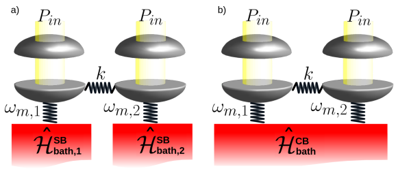
Figure 1: In this work we consider an optomechanical system composed by two optical modes and two mechanical modes, and we allow for a finite mechanical coupling. We consider two dissipation scenarios. a) All the modes of the system dissipate into independent environments (separate baths). b) The mechanical modes dissipate collectively into the same environment (common bath), while the optical modes dissipate into separate baths.

2 Model and methods

2.1 Hamiltonian model

A simple configuration to assess collective or independent forms of dissipation consists of two optomechanical coupled units, as sketched in Fig. 1. We allow for a finite mechanical-mechanical coupling to be compared with dissipative coupling effects, while mixing between optical modes is not addressed here for simplicity. The total Hamiltonian is

$$\hat{\mathcal{H}}_{S}=\hat{\mathcal{H}}_{1}+\hat{\mathcal{H}}_{2}+\frac{k}{2}\big{(}\hat{x}_{1}-\hat{x}_{2}\big{)}^{2},$$ (1)

where $\hat{\mathcal{H}}_{1,2}$ are the Hamiltonians for each optomechanical oscillator and the last term is the mechanical coupling between them. This kind of mechanical coupling can be found for instance in nanoresonators clamped to the same substrate as in Refs. [44, 45, 50], as well as it can be induced optically using off-resonant lasers [51]. Alternatively, interaction with a common (and single) optical field can also induce coupling between mechanical modes of OMs, as in Refs. [11, 14]. The Hamiltonian for each unit of the OMs reads as [52]:

$$\hat{\mathcal{H}}_{j}=\frac{1}{2}m\omega_{m,j}^{2}\hat{x}_{j}^{2}+\frac{1}{2m}\hat{p}_{j}^{2}-\hbar\Delta_{0}\hat{a}^{\dagger}_{j}\hat{a}_{j}+i\hbar\sqrt{\frac{\kappa P_{in}}{\hbar\omega_{L}}}\big{(}\hat{a}^{\dagger}_{j}-\hat{a}_{j}\big{)}-\hbar\frac{\omega_{c}}{L_{om}}\hat{x}_{j}\hat{a}^{\dagger}_{j}\hat{a}_{j},\ \ j=1,2$$ (2)

in the frame rotating with the input laser frequencies [1]. The first two terms of the Hamiltonian correspond to the mechanical elements, described as harmonic oscillators of frequency $\omega_{m,j}$, effective mass $m$, and position and momentum operators $\hat{x}_{j}$, and $\hat{p}_{j}$, where $[\hat{x}_{j},\hat{p}_{j}]=i\hbar$. The third and fourth terms describe the driven optical cavities in the frame rotating at the laser frequency, where $\Delta_{0}=\omega_{L}-\omega_{c}$, $\omega_{c}$ is the cavity resonance frequency, $\omega_{L}$ is the laser frequency, $P_{in}$ is the laser input power, $\kappa$ is the cavity energy decay rate, and $\hat{a}^{\dagger}_{j}$, $\hat{a}_{j}$ are the creation and annihilation operators of the light modes, with $[\hat{a}_{j},\hat{a}^{\dagger}_{j}]=1$. Notice that we make the simplifying assumption of identical optomechanical oscillators except for the mechanical frequencies, in which allowing disparity is essential for the study of synchronization. Finally the last term in Eq. (2) describes the optomechanical coupling with a strength parametrized by the effective optomechanical length $L_{om}$, whose precise definition is system dependent and might involve the particular properties of the interacting optical and mechanical modes (see for instance its definition for optomechanical crystals [53]). Finally we remark that this model is appropriate for many different OMs as long as the parameters of the system, such as $m$ or $L_{om}$, appropriately refer to specific devices (like e.g. examples as diverse as in Refs. [53, 54]).

The optical and mechanical environments are described as an infinite collection of harmonic oscillators in thermal equilibrium. The standard model for the environment of an optical cavity, and the master/Langevin equations describing its dynamics, can be found in many textbooks on open quantum systems [38, 55, 56]. We describe the mechanical environments using the model of Ref. [57], in which the Born-Markov master equations of two coupled $nonidentical$ harmonic oscillators for the CB/SB cases are derived, starting from the following Hamiltonians. In the SB case each mechanical oscillator is coupled to its own reservoir, so there are two different baths described by:

$$\hat{\mathcal{H}}^{SB}_{bath,j}=\sum^{\infty}_{\alpha=1}\hbar\,\omega_{\alpha,j}\hat{r}_{\alpha,j}^{\dagger}\hat{r}_{\alpha,j},\quad\hat{\mathcal{H}}^{SB}_{int,j}=\sum^{\infty}_{\alpha=1}\lambda\,\hat{q}_{\alpha,j}\hat{x}_{j},\quad j=1,2,$$ (3)

where $\hat{r}_{\alpha,j}^{\dagger}$, $\hat{r}_{\alpha,j}$ are the creation and annihilation operators of the bath modes, and $\hat{q}_{\alpha,j}$ their position operators. On the other hand, in the CB case there is only one collective environment for both system units:

$$\hat{\mathcal{H}}^{CB}_{bath}=\sum^{\infty}_{\alpha=1}\hbar\,\omega_{\alpha}\hat{r}_{\alpha}^{\dagger}\hat{r}_{\alpha},\quad\hat{\mathcal{H}}^{CB}_{int}=\sum^{\infty}_{\alpha=1}2\,\lambda\,\hat{q}_{\alpha}\hat{x}_{+},$$ (4)

resulting in coupling through the center of mass coordinate $\hat{x}_{+}=(\hat{x}_{1}+\hat{x}_{2})/\sqrt{2}$ [16, 17, 38, 39, 41, 42, 43, 44]. Notice that we have included a factor two in Eq. (4) to enforce an equal energy damping rate for both models: in SB case two independent channels dissipate, in CB case only one coordinate (center of mass) dissipates, but it is coupled to the bath with double strength $2\lambda$. This allows for a quantitative, not only qualitative, comparison of both dissipation regimes.

2.2 Dimensionless parameters and observables

A set of dimensionless observables and parameters can be introduced similarly to Ref. [6]. First we define the quantities $x_{om}=\kappa L_{om}/\omega_{c}$ and $n_{max}=4P_{in}/\hbar\omega_{L}\kappa$, which we use to achieve a dimensionless time and dimensionless operators of the system:

$$t^{\prime}=\kappa t,\quad\hat{x}_{j}^{\prime}=\frac{\hat{x}_{j}}{x_{om}},\quad\hat{p}_{j}^{\prime}=\frac{\hat{p}_{j}}{m\,\kappa\,x_{om}},\quad\hat{a}_{j}^{\prime}=\frac{\hat{a}_{j}}{\sqrt{n_{max}}},$$ (5)

where the dimensionless quantities are denoted by a prime. Then the following dimensionless parameters appear in the equations of motion:

$$\omega_{m,j}^{\prime}=\frac{\omega_{m,j}}{\kappa},\ \ \Gamma^{\prime}=\frac{\gamma}{\kappa},\ \ K_{c}^{\prime}=\frac{k}{m\kappa^{2}},\ \ \Delta_{0}^{\prime}=\frac{\Delta_{0}}{\kappa},\ \ \mathcal{P}^{\prime}=\frac{4P_{in}\omega_{c}}{mL_{om}^{2}\kappa^{4}}.$$ (6)

Unless stated otherwise we will work with these dimensionless parameters in the following, and thus we can drop the primes.

2.3 Nonlinear classical equations

After defining the set of dimensionless parameters and observables used in this work, we can write down the dimensionless equations describing the classical dynamics of this system [9], both for SB and CB. The classical dynamics can be obtained by the quantum equations of motion taking the first moments and making the approximation of factorizing expectation values of nonlinear terms, as usual. The quantum dynamics can be obtained either from a master equation approach as well as from the quantum Langevin equations of the system (see next section) [1, 56, 57]:

$$\dot{a}_{j}=\bigg{[}i(\Delta_{0}+x_{j})-\frac{1}{2}\bigg{]}a_{j}+\frac{1}{2},\quad j=1,2,$$ (7)

$$\dot{x}_{j}=p_{j},\quad\dot{p}_{j}=-\omega^{2}_{m,j}x_{j}+(-1)^{j}K_{c}(x_{1}-x_{2})-\mathcal{D}_{SB/CB}+\mathcal{P}|a_{j}|^{2},$$ (8)

where variables without hat denote expectation values, e.g., $x=\langle\hat{x}\rangle$. The mechanical dissipation terms are defined as $\mathcal{D}_{SB}=\Gamma p_{j}$ for the separate bath case [9], and $\mathcal{D}_{CB}=\Gamma(p_{1}+p_{2})$ for the common bath case [57].

The dynamical behavior of optomechanical systems can be very diverse depending on the parameter choice [1]. When the mechanical resonator is ’too slow’ with respect to the cavity lifetime (low mechanical quality factor, and $\omega_{m}$ smaller than $\kappa$, in dimensional units), the intracavity power follows adiabatically changes in the mechanical displacement, and a fixed point in which radiation pressure equilibrates with the mechanical restoring force is reached [2]. Otherwise, when the mechanical resonator is able to follow the fast cavity dynamics (high quality factors, and $\omega_{m}$ comparable to $\kappa$), dynamical backaction enables striking phenomena such as damping (cooling) or anti-damping (heating) of the mechanical motion by the optical cavity [1, 58]. In fact optomechanical cooling is enhanced in the red-sideband regime ($\Delta_{0}<0$) whereas anti-damping in the blue-sideband regime ($\Delta_{0}>0$). For enough laser power, $\mathcal{P}$, anti-damping can overcome intrinsic mechanical damping resulting in a dynamical instability and self-sustained oscillations [1, 58]. In these conditions the optomechanical system experiences a supercritical Hopf bifurcation when varying continuously $\Delta_{0}$ from negative to positive values [6, 59]. Moreover, for strong driving a dynamical multistability is found, and self-sustained oscillations are possible even in the red-sideband regime [6]. The regime of self-sustained oscillations has been explored in the context of spontaneous synchronization in presence of independent dissipation for two coupled mechanical units [9] and in Section 3 we are going to address the effect of dissipative coupling (CB).

2.4 Linear quantum Langevin equations

From the above Hamiltonian model and the input-output formalism we can obtain a set of Langevin equations describing the noise driven damped dynamics of the operators [1] (see also the A), that will be used in Sect. 4 to explore a possible improvement of non-classical effects in presence of collective dissipation. We are going to consider the system in a stable and stationary state where a linearized treatment is a suitable approximation for the fluctuations dynamics (for more details see for instance Refs. [1, 34, 60]). Low temperatures and high mechanical and optical quality factors [1] also contribute to maintain low levels of noise (fluctuations). Indeed setting the OMs in a stable fixed point [34, 60] the fluctuation operators can be defined as: $\delta\hat{O}=\langle{O}\rangle_{st}-\hat{O}$, where $\langle{O}\rangle_{st}$ is the constant solution of equations (7) and (8), and the linear equations for the fluctuation operators are:

$$\delta\dot{\hat{Q}}_{j}=-(\langle{x}_{j}\rangle_{st}+\Delta_{0})\delta\hat{P}_{j}-\langle{P}_{j}\rangle_{st}\,\delta\hat{x}_{j}-\frac{1}{2}\delta\hat{Q}_{j}+\sqrt{\frac{\omega_{m}}{\mathcal{P}}}\,\hat{Q}_{in,j},\quad j=1,2,$$ (9)

$$\delta\dot{\hat{P}}_{j}=(\langle{x}_{j}\rangle_{st}+\Delta_{0})\delta\hat{Q}_{j}+\langle{Q}_{j}\rangle_{st}\,\delta\hat{x}_{j}-\frac{1}{2}\delta\hat{P}_{j}+\sqrt{\frac{\omega_{m}}{\mathcal{P}}}\,\hat{P}_{in,j},$$ (10)

$$\delta\dot{\hat{x}}_{j}=\delta\hat{p}_{j}-d^{x}_{SB/CB}+\hat{x}_{in,j},$$ (11)

$$\delta\dot{\hat{p}}_{j}=-\omega^{2}_{m}\delta\hat{x}_{j}+(-1)^{j}K_{c}\big{(}\delta\hat{x}_{1}-\delta\hat{x}_{2}\big{)}-d^{p}_{SB/CB}+\mathcal{P}(\langle{Q}_{j}\rangle_{st}\,\delta\hat{Q}_{j}+\langle{P}_{j}\rangle_{st}\,\delta\hat{P}_{j})+\omega_{m}\,\hat{p}_{in,j}.$$ (12)

In the following we are going to consider the light quadratures $\hat{Q}_{j}=(\hat{a}_{j}+\hat{a}_{j}^{\dagger})/\sqrt{2}$ and $\hat{P}_{j}=i(\hat{a}_{j}^{\dagger}-\hat{a}_{j})/\sqrt{2}$. We also notice that we are considering identical optomechanical oscillators in the study of quantum correlations (Sect. 4). As usual, the fluctuation operators are rescaled by the parameter $\zeta=\tilde{x}_{zpf}/x_{fwhm}$ with $\tilde{x}_{zpf}=\sqrt{\hbar/m\omega_{m}}$, so that $\delta\hat{O}_{new}=\delta\hat{O}_{old}/\zeta$.

The mechanical dissipation terms are:

$$d^{x}_{SB}=\Gamma\delta\hat{x}_{j},\quad d^{p}_{SB}=\Gamma\delta\hat{p}_{j},\quad d^{x}_{CB}=\Gamma\big{(}\delta\hat{x}_{1}+\delta\hat{x}_{2}\big{)},\quad d^{p}_{CB}=\Gamma\big{(}\delta\hat{p}_{1}+\delta\hat{p}_{2}\big{)},$$ (13)

where the known equivalence in position and momentum damping results from the rotating wave approximation in the system-bath coupling, a valid approximation in the limit $\Gamma\ll\omega_{m}$ (i.e. high mechanical quality factors) [38]. In the Markovian limit, the zero mean Gaussian noise terms of equations (9) to (12) are characterized by the following symmetrized correlations [34]:

$$\langle\big{\{}\hat{Q}_{in,j}(t),\hat{Q}_{in,j}(t^{\prime})\big{\}}\rangle = \langle\big{\{}\hat{P}_{in,j}(t),\hat{P}_{in,j}(t^{\prime})\big{\}}\rangle=\delta(t-t^{\prime}),\quad j=1,2,$$ (14)

$$\frac{1}{2}\langle\big{\{}\hat{x}_{in,j}(t),\hat{x}_{in,j}(t^{\prime})\big{\}}\rangle = \frac{1}{2}\langle\big{\{}\hat{p}_{in,j}(t),\hat{p}_{in,j}(t^{\prime})\big{\}}\rangle=\Gamma(2n_{th}+1)\delta(t-t^{\prime}),$$ (15)

where $\{...\,,\,...\}$ denotes anticommutator, $\langle...\rangle$ denotes an ensemble average, $\delta(t-t^{\prime})$ is the Dirac delta, and $n_{th}=(\exp[\hbar\omega_{m}/k_{B}T]-1)^{-1}$ is the phonon occupancy number of the mechanical baths, assumed to be at the same temperature $T$. The light noise correlations for the corresponding quadratures are obtained by considering optical environments at zero temperature for which the only nonvanishing correlations are $\langle\hat{a}_{in,j}(t)\hat{a}^{\dagger}_{in,j}(t^{\prime})\rangle=\delta(t-t^{\prime})$ for $j=1,2$ [34]. In the CB case additional cross-correlations appear:

$$\frac{1}{2}\langle\big{\{}\hat{x}_{in,1}(t),\hat{x}_{in,2}(t^{\prime})\big{\}}\rangle=\frac{1}{2}\langle\big{\{}\hat{p}_{in,1}(t),\hat{p}_{in,2}(t^{\prime})\big{\}}\rangle=\Gamma(2n_{th}+1)\delta(t-t^{\prime}).$$ (16)

Finally we remark that as the fluctuations dynamics is linear and the noise is Gaussian, states initially Gaussian will remain Gaussian at all times [61, 62]. Notably Gaussian states are completely characterized by their first and second moments, which are all encoded in the covariance matrix of the system [61, 62]. Rewriting the Langevin equations (9-12) as $\dot{\vec{R}}=\mathcal{M}\vec{R}+\vec{D}$, where $\vec{R}$ is the vector of the position, momentum, and light quadratures of the system, $\vec{D}$ is the vector containing the noise terms, and $\mathcal{M}$ is the matrix generating the dynamics of the system, the following equation for the covariance matrix can be written down:

$$\dot{\mathcal{C}}=\mathcal{M}\,\mathcal{C}+\mathcal{C}\,\mathcal{M}^{T}+\mathcal{N},$$ (17)

with the covariance matrix and the noise covariance matrix defined respectively as:

$$\mathcal{C}_{ij}(t)=\frac{\langle R_{i}(t)R_{j}(t)+R_{j}(t)R_{i}(t)\rangle}{2},\quad\mathcal{N}_{ij}(t)=\frac{\langle D_{i}(t)D_{j}(t)+D_{j}(t)D_{i}(t)\rangle}{2},$$ (18)

with $i,j=1,...,8$. By solving equation (17) at any time we can completely characterize the quantum correlations present in the system [63, 64].

3 Classical synchronization

In this section we analyze the effects of collective dissipation on the synchronization of the first moments of the system, or classical synchronization. In the SB case classical synchronization has been already studied in Ref. [9], where it has been shown that the OMs described by equations (7) and (8) can synchronize with a locked phase difference either tending to 0, in-phase synchronization, or to $\pi$, anti-phase synchronization. To study the presence of synchronization we integrate numerically equations (7) and (8) in both CB/SB cases and in a parameter region in which the system is self-oscillating. Once the system is in the steady state we compute a synchronization measure. Synchronization is characterized by a Pearson correlation function defined as:

$$C_{x_{1},x_{2}}(t,\Delta t)=\frac{\overline{\delta x_{1}\delta x_{2}}}{\sqrt{\overline{\delta x_{1}^{2}}\,\,\overline{\delta x_{2}^{2}}}},$$ (19)

where the bar represents a time average with time window $\Delta t$, i.e. $\overline{x}=\frac{1}{\Delta t}\int_{t}^{t+\Delta t}ds\,x(s)$, and $\delta x=x(t)-\overline{x}$. This correlation function has proven to be a useful indicator of synchronization both in classical and quantum systems [15, 65]. In particular this measure provides an absolute scale for synchronization strength as it takes values between -1 and 1, where -1 means perfect anti-phase synchronization and 1 perfect in-phase synchronization. Furthermore this measure can be generalized also in presence of time delays accounting for regimes where OMs synchronize with a phase difference depending on the parameter values. In this case two delayed functions, $x_{1}(t)$ and $x_{2}(t+\tau)$, need to be considered in Eq. (19). The best figure of merit accounting for delay is found maximizing the synchronization measure for different values of $\tau$: in particular we take an interval of time $\Delta t$ such that it includes many periodic oscillations, and we compute the correlation function (19) between $x_{1}(t)$ and $x_{2}(t+\tau)$, where $\tau$ is varied between $[0,\mathcal{T}]$, being $\mathcal{T}$ the period of the oscillation. By keeping the maximum correlation $C_{max}$, and the temporal shift at which it occurs $\tau_{max}$, we obtain a measure of the degree or quality of synchronization, $C_{max}$, and the locked phase difference, $\tau_{max}/\mathcal{T}$, in units of $2\pi$.

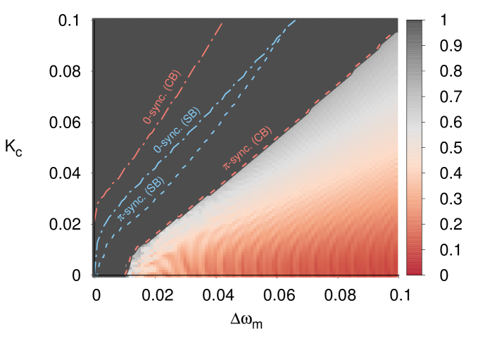
Figure 2: Colorscale: degree of synchronization $C_{max}$ between the average mechanical positions of two coupled OMs for the CB case, as a function of the mechanical frequency detunig, $\Delta\omega_{m}$, and the mechanical coupling, $K_{c}$. The fixed parameters take the following values: $\mathcal{P}=0.36$, $\Delta_{0}=1$, $\Gamma=0.01$, and $\omega_{m,1}=1$ (like in Ref. [9]). Dashed lines indicate the onset of anti-phase synchronization. Dashed-dotted lines indicate the onset of in-phase synchronization. Salmon lines correspond to the CB case, and blue lines to the SB case.

The degree of synchronization accounting for delay, $C_{max}$, as a function of the frequency detuning, $\Delta\omega_{m}=\omega_{m,2}-\omega_{m,1}$, and the mechanical coupling strength, $K_{c}$, is shown in figure 2, where synchronization is found for coupling overcoming detuning between the mechanical oscillators. The case of dissipation in a CB is represented also including a comparison with the SB case studied in Ref. [9] in which a similar synchronization diagram was already observed. In the synchronized regions, $C_{max}\approx 1$, the mechanical elements oscillate at the same frequency describing sinusoidal trajectories with constant amplitude. Conversely, when there is no synchronization ($0\lesssim C_{max}\lesssim 0.6$ in the represented case), the mechanical oscillations have different frequencies and display strong amplitude modulations.

In presence of synchronization two further regimes are recognized depending on whether the locked phase difference tends to $0$ or to $\pi$. At threshold the system first anti-synchronize and by further increasing the coupling for a given detuning there is a transition to in-phase synchronization (respectively, dashed and dashed-dotted lines of figure 2, for both CB (salmon lines) and SB (blue lines)). The comparison allows to identify how collective dissipation favors spontaneous synchronization: indeed, the synchronized area for CB is much larger than for SB, as the first anti-phase synchronization threshold coupling is lowered (salmon and blue dashed ‘$\pi$-sync.’ lines). The anti-phase synchronization regime is also enlarged for CB case as the second threshold to in-phase synchronization increases for CB with respect to SB. The fact the anti-phase synchronization is favored is consistent with the particular dissipation form in the CB case: it is the common coordinate $x_{1}+x_{2}$ that is damped by the environment, see Eq. (8), leading to a ‘preferred’ amplitude of motion in $x_{1}-x_{2}$, and thus an anti-phase locking.

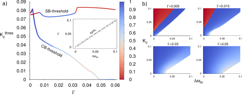
Figure 3: a) Minimum mechanical coupling necessary to synchronize the oscillators, $K_{c}^{thres}$, as a function of the dissipation rate, $\Gamma$. The other parameters are fixed to: $\mathcal{P}=0.36$, $\Delta_{0}=1$, $\omega_{m,1}=1$, and $\Delta\omega_{m}=0.05$. Colorscale: locked phase difference in units of $\pi$. Inset: minimum dissipation rate, $\Gamma$, necessary to synchronize the oscillators in the CB case, for a given detuning, $\Delta\omega_{m}$, with $K_{c}=0$, and the other parameters as in the main panel. The dashed black line corresponds to $\Gamma=\Delta\omega_{m}$. b) Panels: locked phase difference (using the same colorscale as in Fig. 3a) as a function of the mechanical frequency detunig, $\Delta\omega_{m}$, and the mechanical coupling, $K_{c}$, for the CB case. Different values of $\Gamma$ are used ($\Gamma=0.005,0.015,0.03,0.05$), and the other parameters are fixed to $\mathcal{P}=0.36$, $\Delta_{0}=1$, $\omega_{m,1}=1$. White regions correspond to unsynchronized regions.

The effect of dissipation on the synchronization threshold is quantified for CB and SB in Fig. 3, for fixed detuning, looking at the mechanical coupling $K_{c}^{thres}$ needed for the system to synchronize when increasing the damping rate $\Gamma$. This mechanical coupling threshold $K_{c}^{thres}$ is defined as the minimum amount of mechanical coupling, $K_{c}$, needed for the oscillators to synchronize, and can be easily obtained as the synchronization of the system is signaled by a sharp transition of the synchronization indicator from small values (for our parameters below $C_{max}\approx 0.6$ ) to the values around unity that characterize synchronized oscillations. The damping strength does not influence significantly the synchronization threshold in SB case, in stark contrast with the CB case, which is very sensitive to the damping strength and improving significantly when increasing $\Gamma$. The enlargement in the (anti-)synchronization area for the CB case is also displayed in the full parameter plots (Fig. 3b). This clearly shows how the presence of an additional (dissipative) coupling term between the oscillators in the CB case triggers the emergence of spontaneous synchronization. In other words, both reactive and dissipative couplings contribute similarly in overcoming detuning effects in the context of synchronization. Furthermore CB specially favors anti-phase synchronization being the relative motion of the oscillators shielded by damping effects.

An interesting effect of collective dissipation is that actually spontaneous synchronization can emerge even in absence of direct mechanical coupling (see Fig. 2 for $\Delta\omega_{m}\lesssim 0.01$ and Fig. 3a for $\Gamma\gtrsim 0.05$). This is a specific signature of CB dissipation, being indeed not possible between uncoupled OMs with SB, and shows the constructive role played by the dissipative coupling due to CB even in absence of any other optical or mechanical coherent coupling. The threshold for synchronization between decoupled oscillators ($K_{c}=0$) in the CB case is indeed set by the damping strength occurring for $\Gamma$ overcoming detuning effects ($\Delta\omega_{m}$) as nicely shown in the inset of Fig. 3a. We also notice that, for $\Gamma$ small enough, synchronization is always in-phase (red points) while when increasing it different phase (delays) can be favored at threshold (Fig. 3). In particular, in the CB case, the phase-locked difference does not always correspond to in-phase or anti-phase synchronization, as it also takes intermediate values $\sim\pi/2$. This occurs both with (Fig. 3a) and without (inset in Fig. 3a and Fig. 3b) direct mechanical coupling, being more evident for larger dissipation rates (Fig. 3a and b). The exact mechanism behind these $\pi/2$ values of the locked phase-difference is an open question.

4 Asymptotic entanglement and optomechanical cooling

In this section we study the entanglement between mechanical modes in the asymptotic state of the dynamics. As explained in Section 2 we set the system in a stable fixed point and we study the linear fluctuations around the mean state. The stationary state of the fluctuations is independent of the initial conditions and we characterize it obtaining numerically the stationary covariance matrix from equation (17). From this covariance matrix we can compute entanglement between the different degrees of freedom [61, 62], for which we use the logarithmic negativity, a valid entanglement monotone for mixed Gaussian states [61, 62]. Its definition for modes described by quadratures with commutation relations $[q_{1,2},p_{1,2}]=i$ is $E_{N}=\mathrm{max}\{0,-ln\,2\tilde{\nu}_{-}\}$, where $\tilde{\nu}_{-}$ is the smallest symplectic eigenvalue of the partially transposed covariance matrix of the subsystem [62].

One of the main results discussed below is the tight relation between the effective temperature of the mechanical modes and the amount of asymptotic entanglement that is preserved between them: the linear regime in which the system is operated basically consists of four coupled units which in the stationary state reach a given effective temperature depending on the effectivity of the optomechanical cooling. It seems that this effective temperature regulates the entanglement behavior, which is that of a coupled thermal system. Furthermore we find that the CB case has higher mechanical entanglement and is easier to cool down than the SB case, specially when increasing the relative mechanical coupling strength $K_{c}/\omega_{m}^{2}$. We analyze next the dependence of cooling and entanglement on the different system parameters, showing that this is a puzzle with several pieces. At this point we remark that as in the following we are dealing with identical optomechanical oscillators, quantities such as the occupation number of each of the mechanical oscillators ($n_{\mathrm{eff}}$), or the optical-mechanical entanglement between a mechanical mode and its optical mode, are the same for the two optomechanical oscillators.

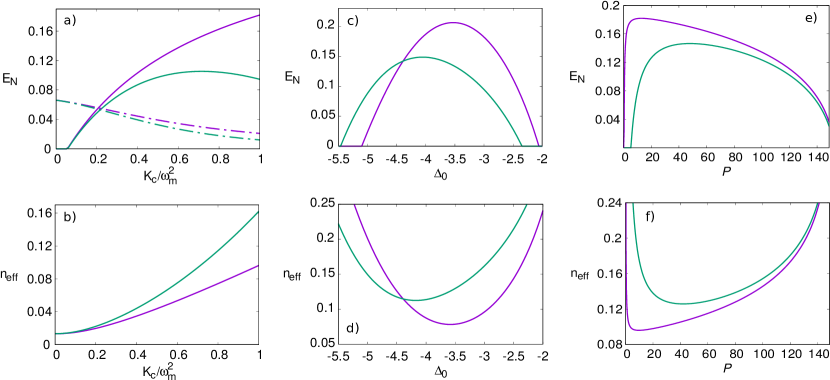
Figure 4: CB case: purple lines. SB case: green lines. Fixed parameters: $\omega_{m}=3$, $Q_{m}=\omega_{m}/\Gamma=10^{5}$ and $\hbar\omega_{m}/k_{B}T=0.1$ ($n_{th}\approx 9.5$). a) Asymptotic entanglement between the mechanical modes (solid lines) and between the mechanical modes and their respective optical modes (dashed-dotted lines) as a function of the ratio $K_{c}/\omega_{m}^{2}$ This is an indicator of the frequency splitting of the normal modes of two coupled oscillators, i.e. $(\Omega_{-}-\Omega_{+})/\omega_{m}\approx K_{c}/\omega_{m}^{2}+O\big{[}(K_{c}/\omega_{m}^{2})^{2}\big{]}$. b) Mechanical occupancy numbers. In a) and b) $\Delta_{0}=-\omega_{m}$ and $\mathcal{P}=12$. c,d) Asymptotic mechanical entanglement and mechanical occupancy numbers with $K_{c}/\omega_{m}^{2}=1$ and $\mathcal{P}=12$. e,f) Asymptotic mechanical entanglement and mechanical occupancy numbers with $K_{c}/\omega_{m}^{2}=1$ and $\Delta_{0}=-\omega_{m}$.

Mechanical coupling $K_{c}$.- We first consider asymptotic entanglement when varying the mechanical coupling between the oscillators. A minimum coupling is needed to attain non-vanishing entanglement between the mechanical modes (solid lines in Fig. 4a), both for CB and SB. Indeed, only above some minimum coupling $K_{c}$ entanglement overcomes heating effects as shown (through the mechanical occupancy number $n_{\mathrm{eff}}$) in Fig. 4b. This is known to occur also in the simplest configuration of a pair of coupled harmonic oscillators at finite temperature [66, 67]. We mention that actually for similar (effective) temperatures and similar mechanical coupling strengths we find that both harmonic and optomechanical systems display similar amounts of entanglement. Slightly above this threshold the build-up of entanglement is similar in presence of CB or SB (Fig. 4a), as also the heating of the mechanical components (Fig. 4b), but further increasing the coupling differences arise and entanglement worsen for SB. This effect is accompanied by a stronger heating in the SB than in the CB case (Fig. 4b). Overall, larger entanglement, as well as better cooling (smaller $n_{\mathrm{eff}}$), are found for the CB case.

From these observations we infer that the mechanical coupling between the oscillators influences their entanglement through two competing mechanisms: on the one hand it is the coupling that entangles the two mechanical oscillators, on the other $K_{c}$ modifies the effective temperature of the oscillators. This is because the normal mode frequencies change with $K_{c}$ reducing their resonance with the optical modes and therefore hindering their cooling (see discussion below and Fig. 5). As the heating produced increasing $K_{c}$ is more pronounced for independent dissipation, best entanglement values are attained in the CB case. This picture is confirmed when looking at ‘light-mirror’ entanglement: $K_{c}$ is not expected to contribute significantly to the ‘light-mirror’ correlations in each OM oscillator, while the effects of heating will still be present. As we see from figure 4a (dashed-dotted lines) the optical-mechanical entanglement is present for all couplings (no threshold) and diminishes when increasing $K_{c}$. Both for CB and SB cases the loss of entanglement is similar to the effective heating (increasing effective temperature) in accordance with the above considerations.

Cavity-laser detuning $\Delta_{0}$.- The detuning $\Delta_{0}$, set to values comparable to the mechanical frequencies, allows for quanta exchange between the very disparate optical and mechanical modes. In this way the optical reservoir, effectively at $T=0$, acts as a heat sink for the mechanical degrees of freedom when the system operates in the red-sideband regime [27, 28]. Thus, resonance between optical and mechanical degrees of freedom controls the effectiveness of the cooling process. Looking at figures 4c and 4d we see that the entanglement between oscillators and their effective temperature display a strong inverse behavior, i.e. as the effective temperature drops the entanglement grows and vice versa, and the maximum of entanglement is very close to the minimum of temperature for both CB/SB cases. This behavior is found also for different temperatures and mechanical couplings. Despite the fact that the optimal $\Delta_{0}$ values for cooling and entanglement are slightly (less than $2\%$) shifted one with respect to the other, the strong anticorrelations between the two curves and the small size of these shifts, make us conclude that the laser detuning $\Delta_{0}$ modifies the asymptotic mechanical entanglement mainly through the degree of optomechanical cooling. We also note that the detuning for optimal cooling in both CB/SB cases is displaced with respect to known values for single OMs $\Delta_{0}\approx-\omega_{m}$ [27, 28] (see discussion on optimal detuning). Finally we note that entanglement and cooling are again enhanced in the CB case, and that the optimal detunings for maximum entanglement are quite different in the CB and SB case (the same applies to the detunings for optimal cooling).

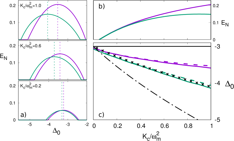
Figure 5: CB case in purple. SB case in green. a) Entanglement for different values of $K_{c}/\omega_{m}^{2}=0.2,0.6,1$ as a function of $\Delta_{0}$ and with $\omega_{m}=3$, $Q_{m}=10^{5}$, $\hbar\omega_{m}/k_{B}T=0.1$ and $\mathcal{P}=12$. Dashed lines at the maxima positions. b) Maximum entanglement for $\Delta_{0}$ as a function of $K_{c}/\omega_{m}^{2}$. c) Solid colored lines: $\Delta_{0}$ maximizing optomechanical cooling as a function of $K_{c}/\omega_{m}^{2}$. Dashed colored lines: $\Delta_{0}$ maximizing mechanical entanglement as a function of $K_{c}/\omega_{m}^{2}$. The black solid line is $\Delta_{0}=-\Omega_{+}$, the black dashed-dotted is $\Delta_{0}=-\Omega_{-}$, and the black cross-line is $\Delta_{0}=-\overline{\Omega}$, defined in the main text.

Laser power $\mathcal{P}$.- Similarly to the case of $\Delta_{0}$, $\mathcal{P}$ modifies the mechanical entanglement mainly by modifying the degree of optomechanical cooling as it follows from the strong inverse behavior of figures 4e and 4f. Recall from the linear quantum Langevin equations, that $\mathcal{P}$ has the role of a coupling strength between the optical and mechanical quantum fluctuations. It is then to be expected that optomechanical cooling improves with $\mathcal{P}$. However, when $\mathcal{P}$ becomes very high, it is known [28, 68] that optical and mechanical modes begin to hybridize and heating from quantum backaction noise enters the scene. Thus at first higher $\mathcal{P}$ implies an enhancement of the optomechanical cooling effect, since this coupling parametrizes the strength of the optomechanical cooling rate [27, 28]. As $\mathcal{P}$ is further increased, the regime of strong coupling is reached and heating of the mechanical modes by radiation pressure becomes important. The competition between these two effects leads to a minimum of $n_{\mathrm{eff}}$ as a function of the optomechanical coupling strength, as derived for a single OMs in Refs. [28, 68] and observed in figure 4f. Finally, the CB case requires less power to achieve the same cooling as compared to the SB case.

Optimal detuning.- As we have observed in the discussion of figures 4c and d, the asymptotic mechanical entanglement changes with $\Delta_{0}$ mainly because of the effectiveness of the optomechanical cooling process. The detuning optimizing each process indeed takes very similar values as mentioned above. In figure 5 we analyze in more detail the detunings $\Delta_{0}$ which are optimal for optomechanical cooling and mechanical entanglement as a function of the relative mechanical coupling strength $K_{c}/\omega_{m}^{2}$, and address some of the differences between the CB/SB cases that have been pointed out in the above discussions. In Fig. 5a we can see that as $K_{c}/\omega_{m}^{2}$ increases, the $\Delta_{0}$ maximizing entanglement is shifted towards more negative values. In figure 5b we have plotted the maximum entanglement for the optimal value of $\Delta_{0}$ as a function of $K_{c}/\omega_{m}^{2}$, and we see that it increases in both cases and it is larger for the CB case. We note that the increase with $K_{c}/\omega_{m}^{2}$ is similar to that in 4a, but that here we compute the value at the optimal $\Delta_{0}$ for each $K_{c}/\omega_{m}^{2}$, $\textrm{max}_{\Delta_{0}}{E_{N}(K_{c}/\omega_{m}^{2})}$ , thus increasing a bit the level of achieved entanglement. Analogous results are obtained when studying the detuning for minimum effective temperature (not shown here).

In figure 5c we address the question of how the detunings that maximize entanglement or minimize the effective temperature vary with the relative mechanical coupling strength. In particular we plot the $\Delta_{0}$ that optimizes cooling (solid lines) and the one that optimizes entanglement (dashed lines) as a function of $K_{c}/\omega_{m}^{2}$. The solid black line corresponds to $\Delta_{0}=-\Omega_{+}$, the dashed-dotted line to $\Delta_{0}=-\Omega_{-}$, and the cross-line to $\Delta_{0}=-\overline{\Omega}=-(\Omega_{+}+\Omega_{-})/2$. Where $\Omega_{\pm}$ are the frequencies of the normal modes of the isolated mechanical system $x_{\pm}=(x_{1}\pm x_{2})/\sqrt{2}$ (i.e. without optomechanical coupling), and which take the values $\Omega_{+}=\omega_{m}$ and $\Omega_{-}=\sqrt{\omega_{m}^{2}+2K_{c}}$. From this figure it is appreciated that the shift between the optimal detunings for cooling and entanglement increases slightly with the mechanical coupling, but it remains small in all the range both for CB and SB. We also observe that in the SB case, the optimal strategy for cooling is to set ($\Delta_{0}\approx-\overline{\Omega}$), and thus the minimum mechanical effective temperature is achieved when both mechanical normal modes (of the isolated system) are cooled at the same rate. Notice that given the small difference between the detunings optimizing each quantity, the same strategy applies, to a good approximation, to obtain the maximum entanglement. On the other hand, in the CB case the optimal $\Delta_{0}$ for cooling and entanglement is shifted towards $-\Omega_{+}$, consistent with the fact that dissipation enters through this coordinate. Why is it then not the case that the optimal detuning coincides with $\Omega_{+}$? Well, the common coordinate $x_{+}$ is a normal mode of the isolated mechanical system, but it is not of the full optomechanical system, so $x_{+}$ and $x_{-}$ are coupled through the optical degrees of freedom. This is why it is necessary to cool both coordinates, although it is more important to cool the one that dissipates most ($x_{+}$). In fact, as we increase $K_{c}/\omega_{m}^{2}$, the role of the optomechanical coupling is diminished, moving the optimal detuning towards $\Omega_{+}$. This also explains why the SB case is harder to cool than the CB one: in SB we need to address both normal modes $x_{\pm}$ with a single laser frequency, whereas for CB it is better to address only $x_{+}$.

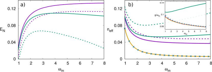
Figure 6: CB case: purple lines. SB case: green lines. Solid lines: $Q_{m}=10^{5}$, $\hbar\omega_{m}/k_{B}T=0.1$ ($n_{th}\approx 9.5$). Dashed lines: $Q_{m}=2\cdot 10^{5}$, $\hbar\omega_{m}/k_{B}T=0.01$ ($n_{th}\approx 99.5$). Maximum entanglement (a) and minimum phonon number (b) optimized with respect to $\mathcal{P}$ (or equivalently with respect to $g/\omega_{m}$, defined in the main text) and varying $\omega_{m}$, with $K_{c}/\omega_{m}^{2}=0.5$, and $\Delta_{0}=-\omega_{m}$. Inset: optimal relative linear optomechanical coupling ($g/\omega_{m}$) at which the minimum phonon number is achieved, for the low temperature case. In b) and in the inset the case of a single optomechanical oscillator has been plotted: yellow solid lines have been obtained numerically, blue cross-lines correspond to the analytical expressions of Ref. [68].

Resolved sideband.- In the following we explore mechanical entanglement (Fig. 6a) and optomechanical cooling (Fig. 6b) as we go deeper into the resolved sideband regime $\omega_{m}>1$, where the parameter $\omega_{m}$ measures how well the linewidth of the optical modes resolves the frequency of the mechanical ones. It is known that the efficiency of the cooling process of a single OM increases initially as $\omega_{m}$ increases [27, 28, 68] (recall that $\omega_{m}/\kappa\mapsto\omega_{m}$ in our dimensionless units, see Sect. 2.2), and thus lower phonon numbers can be achieved when the intracavity power is adjusted optimally [68]. It is then interesting to analyze whether increasing $\omega_{m}$ can enhance cooling and entanglement in the CB/SB cases too. The maximal mechanical entanglement and the minimal mechanical occupancy number optimized in terms of $\mathcal{P}$ for each value of $\omega_{m}$ are displayed in figure 6.

In figure 6a (b), we can see how for the CB case the maximal entanglement (minimal occupancy number) increases (decreases) as $\omega_{m}$ is increased. The SB case at first behaves as the CB case, but for larger $\omega_{m}$ maximal entanglement begins to diminish and the phonon number increases. Notice that again the asymptotic mechanical entanglement and the effective mechanical temperature are strongly anticorrelated following an inverse behavior, in both CB/SB cases. The increase of the minimum effective temperature in the SB case is more evident in the high temperature case (dashed lines Fig. 6a and b), and occurs even at optimal detuning $\Delta_{0}=-\overline{\Omega}$ (not shown here). The difference between CB and SB cases can be explained as follows: for CB cooling the coordinate $x_{+}$ (by setting $\Delta_{0}=-\omega_{m}=-\Omega_{+}$) is almost optimal, and the more we resolve this frequency with our optical modes the better. For SB however, we need to cool both $x_{+}$ and $x_{-}$, but this has to be done with a single optical frequency: the result is that the better we address $\Omega_{+}$, the worse we address $\Omega_{-}$ which gets heated up. Thus in a SB situation it will be more appropriate to have one optical mode targeted at $\Delta_{1}=-\Omega_{+}$, and another at $\Delta_{2}=-\Omega_{-}$, provided we can resolve the difference between $\Omega_{+}$ and $\Omega_{-}$ which requires high mechanical couplings or very low $\kappa$.

In order to point out further differences between the CB/SB cases it is also interesting to study the relative linear optomechanical coupling, $g/\omega_{m}$ (with $g=(\omega_{c}\tilde{x}_{zpf}/L_{om})\sqrt{0.5\langle{a^{\dagger}a}\rangle_{st}}$ [1], in dimensional units), at which optimal cooling is achieved (inset Fig. 6b). From this figure we can observe that as we operate the system deeper in the resolved sideband regime (larger $\omega_{m}$) this optomechanical coupling for optimal cooling diminishes in the CB case. This is so because the exchange between optical and mechanical modes is more efficient, and it is the case both for one OM (yellow solid lines and blue cross-lines) [68], and for the CB case (where addressing $x_{+}$ matters most). In fact, if we increase it too much, we end up heating the mechanical modes due to radiation pressure as shown in figure 4f and in Refs. [28, 68]. Peculiarly, in the SB case, the optimal $g/\omega_{m}$ increases monotonically with $\omega_{m}$. This can be interpreted as follows: as before, the more we resolve, the worse we cool one of the coordinates $x_{\pm}$; the interesting thing is that this effect is initially counteracted by increasing $g/\omega_{m}$ (see small values of $\omega_{m}$, Fig. 6b), which increases the range of frequency that the mechanical mode is able to exchange energy with the optical modes. This is just the well-known fact that stronger couplings allow for resonance with further detuned frequencies, which here counteracts the decreasing optical linewidth. However, as a side effect, radiation pressure heating also grows with the optomechanical coupling, and thus the maximum achievable entanglement (degree of cooling) eventually decreases as shown in figure 6a and b.

For a more quantitative discussion of cooling we simulate the case of a single OM (yellow solid lines and blue cross-lines, Fig. 6b and inset), modeled by equations (9) to (12) for one of the two OMs in the SB case and with $K_{c}=0$. The case of a single OM is studied in Ref. [68], where the optimization of the cooling process in terms of the linear optomechanical coupling is addressed. This is equivalent to what it is shown in figure 6b and in the inset, and we plot their results (Eq. (6) and below of [68]) in blue cross-lines, using the parameters of the low temperature case. We have also obtained the same quantities numerically (yellow solid lines) finding good agreement between the analytical expressions of [68] and the exact results. Comparing the single OM case and the CB case, we find that they follow very similar behaviors both for the minimal occupancy number as well as for the optimal $g/\omega_{m}$ for cooling. In particular, lower phonon numbers are achieved in the single OM case, while the optimal $g/\omega_{m}$ for cooling takes very close values in both cases. On the contrary, the behavior displayed in the SB case is qualitatively different as discussed above. The similitudes between the single OM case and the CB case reinforce the the overall idea that in the CB case we mainly need to address only one dissipative mode: $x_{+}$.

5 Discussion and conclusions

Miniaturization and dense packing of optomechanical devices can give rise to collective effects in dissipation [17], what we have called here common bath (CB), in contrast to the widely used separate baths (SB) dissipation. We have explored the consequences of this form of dissipation in two interesting facets of these kind of nonlinear systems: classical synchronization and steady-state quantum correlations. We have found that the parameter range where synchronization occurs is notably enlarged for CB, and also that in the CB case more dissipation can be beneficial, leading to synchronization even in the absence of mechanical coupling as both the dissipative coupling and the coherent one lead to synchronization between detuned mechanical elements.

With respect to steady-state entanglement of mechanical motion, we have found that the CB case requires less input laser power, because it is more effectively used for cooling, yielding higher levels of entanglement. This can be understood when considering that in this case it is possible to address only the $x_{+}$ mechanical eigenmode, which is the only one dissipating, whereas for SB both modes dissipate equally. This easy picture is quantitatively shown to hold exploring different parameter regions. Furthermore we have shown that going to the resolved sideband regime, the CB case gets monotonically better entanglement and cooling, whereas in SB it improves only up to a point, after which it begins to worsen. This is also due to the inability to cool both eigenmodes with a perfectly resolved sideband at only one of the eigenfrequencies, for which we also propose a two-tone cooling scheme as solution.

As stated in the introduction, a collective dissipation channel is found to be the dominant one in the optomechanical setup of references [44, 45], consisting on the emission of elastic radiation by the common mechanical mode $x_{+}$, and thus being analogous to our CB model. Moreover the fact that this same mechanism is observed in other mechanical oscillators with a similar geometry [48, 49], indicates that collective dissipation is relevant in closely clamped mechanical resonators. Despite the mechanical coupling strength in this device [44, 45] is an order of magnitude smaller than the regime studied here, it is possible to increase it up to the analyzed values by reducing the separation of the beams’ clamping points and increasing the size of the overhang or common substrate, as shown in Ref. [69]. Interestingly this last point suggests that strong mechanical coupling and collective dissipation might go hand in hand. On the other hand, a complementary approach consists on inducing the mechanical coupling by strongly driving the system with off-resonant lasers [51].

In this work we have chosen to study the particular collective dissipation channel $x_{+}$ motivated by the numerous previous works studying this particular type of dissipation emerging from microscopic physical models in different contexts, starting from works on superradiance [41]. Furthermore this collective dissipation has actually been reported in some mechanical platforms as discussed in the introduction [44, 45, 48, 49]. However, other forms of collective dissipation are also possible: $x_{-}$ dissipation can arise in microscopic lattice models [17], and it has been reported in certain systems of trapped ions [70], while more complex forms of collective jumps are considered in [40]. Moreover, quantum correlations and quantum synchronization for $x_{-}$ CB dissipation have been studied both for harmonic oscillators [16, 57], for two level systems [43], and quantum Van der Pol oscillators [20, 21]. In general, it would be interesting to study the robustness of our results also when both collective and individual dissipation channels are present, as this is probably the most common case in experiments.

Finally we discuss the experimental feasibility of the chosen parameters values, noticing that most of them have been reached in experimental platforms (see Ref. [1] section IV for a review on the subject). Specifically, the dimensionless laser power is fixed to $\mathcal{P}=12$, which in terms of the more commonly quoted $g$, is $g/\omega_{m}\approx 0.079$, and when varied takes values at most of $g/\omega_{m}\approx 0.19$ in figure 6, or $g/\omega_{m}\approx 0.37$ when the dynamical instability is reached in figures 4e,f. The values ranges in Fig. 4 have been achieved for instance in the experimental setups of references [71, 72, 73], with the exception of the highest range values explored for $\mathcal{P}$ and $K_{c}/\omega_{m}^{2}$, for which previous considerations hold. The resolved sideband regime has been reached in numerous optomechanical devices, from the GHz mechanical frequencies of optomechanical crystals [53], to MHz frequencies in microtoroidal and LC resonators where values such as $\omega_{m}/\kappa\approx 11$ [72] or $\omega_{m}/\kappa\approx 63$ [73] are reported. Moreover in optimized optomechanical crystals [29, 74] bath phononic occupancies between 10 and 100 are reported for GHz mechanical modes, together with mechanical quality factors of the order of $Q_{m}\sim 10^{4}-10^{6}$. Therefore, based on an analysis of actual state-of-the-art systems [1], this study represents a first step in establishing dynamical and quantum effects of collective dissipation expected to play a key role towards miniaturization of optomechanical devices.

Acknowledgments.- This work has been supported by the EU through the H2020 Project QuProCS (Grant Agreement 641277), by MINECO/AEI/FEDER through projects NoMaQ FIS2014-60343-P, QuStruct FIS2015-66860-P and EPheQuCS FIS2016-78010-P.

Appendix A Derivation of the Langevin equations for the CB case

In this appendix we write down the main steps to derive the Langevin equations for the mechanical oscillators in the CB case. Notice that in this section we are not using the dimensionless variables and parameters introduced in Section 2.2. As usual we assume the cavities and the oscillators to dissipate independently so that we can derive the Langevin equations separately, as if there was no optomechanical coupling [1, 75]. First we write down the mechanical Hamiltonian in the normal mode basis together with the bath Hamiltonians written in equation (4):

$$\mathcal{H}=\frac{1}{2}m(\Omega_{+}^{2}\hat{x}_{+}^{2}+\Omega_{-}^{2}\hat{x}_{-}^{2})+\frac{1}{2m}\big{(}\hat{p}_{+}^{2}+\hat{p}_{-}^{2}\big{)}+2\lambda\sum_{\alpha=1}^{\infty}\hat{x}_{+}\hat{q}_{\alpha}+\hat{\mathcal{H}}^{CB}_{bath},$$ (20)

where we recall that we are assuming identical oscillators, and thus $\Omega_{+}=\omega_{m}$, $\Omega_{-}=\sqrt{\omega_{m}^{2}+2k/m}$. Making the rotating wave approximation in the system-bath coupling and writing the Hamiltonian using the creation and annihilation operators we arrive to:

$$\mathcal{H}=\hbar\Omega_{+}\hat{b}_{+}^{\dagger}\hat{b}_{+}+\hbar\Omega_{-}\hat{b}_{-}^{\dagger}\hat{b}_{-}+2\gamma\sum_{\alpha=1}^{\infty}\hbar(\hat{b}_{+}^{\dagger}\hat{r}_{\alpha}+\hat{b}_{+}\hat{r}_{\alpha}^{\dagger})+\hat{\mathcal{H}}^{CB}_{bath},$$ (21)

where $2\gamma$ is the CB dissipation rate which is twice the SB one $\gamma$. Now we can obtain the Langevin equations of motion for the modes $x_{\pm}$ following the standard input-ouput formalism [76]:

$$\dot{\hat{b}}_{+}=-i\Omega_{+}\hat{b}_{+}-2\gamma\hat{b}_{+}+\sqrt{4\gamma}\hat{b}_{in},\quad\dot{\hat{b}}_{-}=-i\Omega_{-}\hat{b}_{-},$$ (22)

$$\dot{\hat{b}}^{\dagger}_{+}=i\Omega_{+}\hat{b}_{+}^{\dagger}-2\gamma\hat{b}_{+}^{\dagger}+\sqrt{4\gamma}\hat{b}_{in}^{\dagger},\quad\dot{\hat{b}}^{\dagger}_{-}=i\Omega_{-}\hat{b}_{-}^{\dagger},$$ (23)

where the equations for the mode $x_{-}$ are just the Heisenberg equations of motion, since this mode is not coupled to a thermal bath. In the Markovian limit the zero mean Gaussian noise terms are characterized by the following correlations [34]:

$$\langle\hat{b}_{in}^{\dagger}(t)\hat{b}_{in}(t^{\prime})\rangle=n_{th}\delta(t-t^{\prime}),\quad\langle\hat{b}_{in}(t)\hat{b}^{\dagger}_{in}(t^{\prime})\rangle=(n_{th}+1)\delta(t-t^{\prime}),$$ (24)

where $n_{th}$ is the thermal occupancy of the phonon bath defined previously. From these equations we can obtain the equations for the position and momentum operators:

$$\dot{\hat{x}}_{+}=\frac{\hat{p}_{+}}{m}-2\gamma\hat{x}_{+}+\sqrt{4\gamma}\,\tilde{x}_{zpf}\big{[}\frac{\hat{b}_{in}+\hat{b}_{in}^{\dagger}}{\sqrt{2}}\big{]},\quad\dot{\hat{x}}_{-}=\frac{\hat{p}_{-}}{m},$$ (25)

$$\dot{\hat{p}}_{+}=-m\Omega_{+}^{2}\hat{x}_{+}-2\gamma\hat{p}_{+}+\sqrt{4\gamma}\,m\Omega_{+}\tilde{x}_{zpf}\big{[}i\frac{\hat{b}^{\dagger}_{in}-\hat{b}_{in}}{\sqrt{2}}\big{]},\quad\quad\dot{\hat{p}}_{-}=-m\Omega_{-}^{2}\hat{x}_{-}.$$ (26)

Finally we move to the coupled oscillators picture, where $\hat{x}_{\pm}=(\hat{x}_{1}\pm\hat{x}_{2})/\sqrt{2}$ and $\hat{p}_{\pm}=(\hat{p}_{1}\pm\hat{p}_{2})/\sqrt{2}$, obtaining:

$$\dot{\hat{x}}_{j}=\frac{\hat{p}_{j}}{m}-\gamma(\hat{x}_{1}+\hat{x}_{2})+\tilde{x}_{zpf}\hat{x}_{in},\quad j=1,2$$ (27)

$$\dot{\hat{p}}_{j}=-m\omega_{m}^{2}\hat{x}_{j}-\gamma(\hat{p}_{1}+\hat{p}_{2})+(-1)^{j}k(\hat{x}_{1}-\hat{x}_{2})+m\omega_{m}\tilde{x}_{zpf}\hat{p}_{in},$$ (28)

where we have defined $\hat{x}_{in}=\sqrt{\gamma}(\hat{b}_{in}+\hat{b}_{in}^{\dagger})$ and $\hat{p}_{in}=i\sqrt{\gamma}(\hat{b}_{in}^{\dagger}-\hat{b}_{in})$. From these equations we can obtain equations (11) and (12) by coupling the oscillators to the cavities and applying the nondimensionalization/rescaling procedure described in Section 2.2. Furthermore, note that as the noise terms are the same for both oscillators there appear the cross-correlations defined in equation (16).

References

References

- [1] M. Aspelmeyer, T. J. Kippenberg, F. Marquardt, Rev. Mod. Phys. 86, 1391 (2014).
- [2] P. Meystre, E. M. Wright, J. D. McCullen, E. Vignes, J. Opt. Soc. B 2, 1830 (1985).
- [3] A. Dorsel, J. D. McCullen, P. Meystre, E. Vignes, H. Walther, Phys. Rev. Lett. 51, 1550 (1983).
- [4] T. Carmon, H. Rokhsari, L. Yang, T. J. Kippenberg and K. J. Vahala, Phys. Rev. Lett. 94, 223902 (2005).
- [5] T. J. Kippenberg, H. Rokhsari, T. Carmon, A. Scherer and K. J. Vahala, Phys. Rev. Lett. 95, 033901 (2005).
- [6] F. Marquardt, J. G. E. Harris, and S. M. Girvin, Phys. Rev. Lett. 96, 103901 (2006).
- [7] M. Ludwig, C. Neuenhahn, C. Metzeger, A. Ortlieb, I. Favero, K. Karrai and F. Marquardt, Phys. Rev. Lett. 101, 133903 (2008).
- [8] A. G. Krause, J. T. Hill, M. Ludwig, A. H. Safavi-Naeini, J. Chan, F. Marquardt, and O. Painter, Phys. Rev. Lett. 115, 233601 (2015).
- [9] G. Heinrich, M. Ludwig, J. Qian, B. Kubala, and F. Marquardt, Phys. Rev. Lett. 107, 043603 (2011).
- [10] R. Lauter, C. Brendel, S. J. M. Habraken, F. Marquardt, Phys. Rev. E 92, 012902 (2015).
- [11] C. A. Holmes, C. P. Meaney, and G. J. Milburn, Phys. Rev. E 85, 066203 (2012).
- [12] M. Zhang, G. S. Wiederhecker, S. Manipatruni, A. Barnard, P. McEuen, and M. Lipson, Phys. Rev. Lett. 109, 233906 (2012).
- [13] M. Bagheri, M. Poot, L. Fan, F. Marquardt, and H. X. Tang, Phys. Rev. Lett. 111, 213902 (2013).
- [14] M. Zhang, S. Shah, J. Cardenas, and M. Lipson, Phys. Rev. Lett. 115, 163902 (2016).
- [15] F. Galve, G. L. Giorgi, R. Zambrini, ‘Quantum correlations and synchronization measures’, in “Lectures on general quantum correlations and their applications”, Editors: F. Fanchini, D. Soares Pinto, G. Adesso (Springer 2017).
- [16] G. L. Giorgi, F. Galve, G. Manzano, P. Colet, and R. Zambrini, Phys. Rev. A 85, 052101 (2012).
- [17] F. Galve, A. Mandarino, M. G. A. Paris, C. Benedetti, and R. Zambrini, Sci Rep. 7, 42050 (2017).
- [18] G. Manzano, F. Galve, G.L. Giorgi, E. Hernández-García, R. Zambrini, Sci. Reps. 3, (2013).
- [19] A. Mari, A. Farace, N. Didier, V. Giovannetti, and R. Fazio, Phys. Rev. Lett. 111, 103605 (2013).
- [20] T. E. Lee, C. -K. Chan, and S. Wang, Phys. Rev. E 89, 022913 (2014).
- [21] S. Walter, A. Nunnenkamp, and C. Bruder, Ann. Phys. 527, 131 (2015).
- [22] G. L. Giorgi, F. Plastina, G. Francica, and R. Zambrini, Phys. Rev. A 88, 042115 (2013).
- [23] B. Bellomo, G. L. Giorgi, G. M. Palma, and R. Zambrini, Phys. Rev. A 95, 043807 (2017).
- [24] M. Ludwig, and F. Marquardt, Phys. Rev. Lett. 111, 073603 (2013).
- [25] T. Weiss, A. Kronwald, and F. Marquardt, New J. Phys. 18, 013043 (2016).
- [26] F. Bemani, A. Motazedifard, R. Roknizadeh, M. H. Naderi, and D. Vitali, Phys. Rev. A 96, 023805 (2017)
- [27] I. Wilson-Rae, N. Nooshi, W. Zwerger, T. J. Kippenberg, Phys. Rev. Lett. 99, 093901 (2007).
- [28] F. Marquardt, J. P. Chen, A. A. Clerk, and S. M. Girvin, Phys. Rev. Lett. 99, 093902 (2007).
- [29] J. Chan, T. P. M. Alegre, A. H. Safavi-Naeini, J. T. Hill, A. Krause, S. Gröblacher, M. Aspelmeyer, O. Painter, Nature (London) 478, 89 (2011).
- [30] J. D. Teufel, T. Donner, D. Li, J. W. Harlow, M. S. Allman, K. Cicak, A. J. Sirois, J. D. Whittaker, K. W. Lehnert, R. W. Simmonds, Nature (London) 475, 359 (2011).
- [31] T. A. Palomaki, J. D. Teufel, R. W. Simmonds, K. W. Lehnert, Science 342, 710 (2013).
- [32] E. E. Wollman, C. U. Lei, A. J. Weinstein, J. Suh, A. Kronwald, F. Marquardt, A. A. Clerk, K. C. Schwab, Science 349, 952 (2015).
- [33] R. Riedinger, S. Hong, R. A. Norte, J. A. Slater, J. Shang, A. G. Krause, V. Anan Nature (London) 530, 313 (2016).
- [34] D. Vitali, S. Gigan, A. Ferreira, H. R. Bohm, P. Tombesi, A. Guerreiro, V. Vedral, A. Zeilinger, and M. Aspelmeyer, Phys. Rev. Lett. 98, 030405 (2007).
- [35] C. Genes, A. Mari, P. Tombesi, and D. Vitali, Phys. Rev. A 78, 032316 (2008).
- [36] M. Ludwig, K. Hammerer, and F. Marquardt, Phys. Rev. A 82, 012333 (2010).
- [37] M. J. Hartmann, and M. B. Plenio, Phys. Rev. Lett. 101, 200503 (2008).
- [38] H. -P. Breuer, and F. Petruccione, The Theory of Open Quantum Systems (Oxford University Press, Oxford, 2003).
- [39] D. A. Lidar, Adv. Chem. Phys. 154, 295 (2014).
- [40] S. Diehl, A. Micheli, A. Kantian, B. Kraus, H. P. Büchler, and P. Zoller, Nat. Phys. 4, 878 (2008).
- [41] R. H. Dicke, Phys. Rev. 93, 99 (1954).
- [42] J. P. Paz, and A. J. Roncaglia, Phys. Rev. Lett. 100, 220401 (2008).
- [43] F. Galve, R. Zambrini, Coherent and radiative couplings through finite-sized structured environments arXiv:1705.07883
- [44] X. Sun, J. Zheng, M. Poot, C. W. Wong, H. X. Tang, Nano Lett. 12, 2299 (2012).
- [45] J. Zheng, X. Sun, Y. Li, M. Poot, A. Dadgar, N. N. Shi, W. H. P. Pernice, H. X. Tang, and C. W. Wong, Opt. Express 20, 26486 (2012).
- [46] A. H. Safavi-Naeini, J. T. Hill, S. Meenehan, J. Chan, S. Groblacher, and O. Painter, Phys. Rev. Lett. 112, 153603 (2014).
- [47] T. P. Mayer Alegre, A. H. Safavi-Naeini, M. Winger, O. Painter, Opt. Express 19, 5658 (2011).
- [48] A. Naber, J. Microsc. 194, 307 (1999).
- [49] A. Castellanos-Gomez, N. Agrait, and G. Rubio-Bollinger, Ultramicroscopy 111, 186 (2011).
- [50] Q. Lin, J. Rosenberg, D. Chang, R. Camacho, M. Eichenfield, K. J. Vahala, and O. Painter, Nat. Photonics 4, 236 (2010).
- [51] M. Schmidt, M. Ludwig, F. Marquardt, New J. Phys. 14, 125005 (2012).
- [52] C. K. Law, Phys. Rev. A 51, 2537 (1995).
- [53] M. Eichenfield, J. Chan, R. M. Camacho, K. J. Vahala, O. Painter, Nature 462, 78 (2009).
- [54] M. Pinard, Y. Hadjar, and A. Heidmann, Eur. Phys. J. D 7, 107 (1999).
- [55] H. J. Carmichael, An Open Systems Approach to Quantum Optics, Lecture Notes in Physics – New Series m: Mono-graphs (Springer, Berlin, 1993).
- [56] C. W. Gardiner, Quantum Noise (Springer-Verlag, Berlin, 1991).
- [57] F. Galve, G. L. Giorgi, R. Zambrini, Phys. Rev. A 81, 062117 (2010).
- [58] T. J. Kippenberg, K. J. Vahala, Opt. Express 15, 17172 (2007).
- [59] M. Ludwig, B. Kubala, and F. Marquardt, New J. Phys. 10, 095013 (2008).
- [60] C. Fabre, M. Pinard, S. Bourzeix, A. Heidmann, E. Giacobino, and S. Reynaud, Phys. Rev. A 49, 1337 (1994).
- [61] G. Adesso, and F. Illuminati, J. Phys. A: Math. Theor. 40, 7821 (2007).
- [62] S. Olivares, Eur. Phys. J. Spec. Top. 203, 3 (2012).
- [63] A. Mari and J. Eisert, Phys. Rev. Lett. 103, 213603 (2009).
- [64] A. Farace and V. Giovannetti, Phys. Rev. A 86, 013820 (2012).
- [65] A. Pikovsky, M. Rosenblum, and J. Kurths. Synchronization: A Universal Concept in Nonlinear Sciences (Cambridge edition, 2001).
- [66] J. Anders, Phys. Rev. A 77, 062102 (2008).
- [67] F. Galve, L. A. Pachon, and D. Zueco, Phys. Rev. Lett. 105, 180501 (2010).
- [68] J. M. Dobrindt, I. Wilson-Rae and T. J. Kippenberg, Phys. Rev. Lett 101, 263602 (2008).
- [69] E. Gil-Santos, D. Ramos, V. Pini, M. Calleja, and J. Tamayo, Appl. Phys. Lett. 98, 123108 (2011).
- [70] F. Galve, J. Alonso and R. Zambrini, Probing the orientation and spatial correlations of dipole fluctuators on the surfaces of ion traps arXiv:1703.09657.
- [71] S. Groblacher, K. Hammerer, M. R. Vanner, and M. Aspelmeyer, Nature (London) 460, 724 (2009).
- [72] E. Verhagen, S. Deléglise, S. Weis, A. Schliesser, and T. J. Kippenberg, Nature (London) 482, 63 (2012).
- [73] J. D. Teufel, Dale Li, M. S. Allman, K. Cicak, A. J. Sirois, J. D. Whittaker, and R. W. Simmonds, Nature (London) 471, 204 (2011).
- [74] J. Chan, A. H. Safavi-Naeini, J. T. Hill, S. Meenehan, O. Painter, Appl. Phys. Lett. 101, 081115 (2012).
- [75] V. Giovannetti and D. Vitali, Phys. Rev. A 63, 023812 (2001).
- [76] D. Walls and G. J. Milburn, Quantum Optics (Heidelberg: Springer, 2008).