The Maximum Dissipation Principle in Rigid-Body Dynamics with Purely Inelastic Impacts

Abstract

Formulating a consistent theory for rigid-body dynamics with impacts is an intricate problem. Twenty years ago Stewart published the first consistent theory with purely inelastic impacts and an impulsive friction model analogous to Coulomb friction. In this paper we demonstrate that the consistent impact model can exhibit multiple solutions with a varying degree of dissipation even in the single-contact case. Replacing the impulsive friction model based on Coulomb friction by a model based on the maximum dissipation principle resolves the non-uniqueness in the single-contact impact problem. The paper constructs the alternative impact model and presents integral equations describing rigid-body dynamics with a non-impulsive and non-compliant contact model and an associated purely inelastic impact model maximizing dissipation. An analytic solution is derived for the single-contact impact problem. The models are then embedded into a time-stepping scheme. The macroscopic behaviour is compared to Coulomb friction in a large-scale granular flow problem.

1 Introduction

Simulating mechanical systems on computers requires a model for describing the dynamics of the mechanical parts. Models that can describe the deformation of the mechanical parts require a high number of parameters to describe the deformation. If the core of the mechanical parts can be assumed to not deform under the considered loads, the parameters describing the state of a mechanical part can be reduced to that of a rigid body: An invariant shape with an associated mass and principal moments of inertia as well as the spatial orientation, position, linear and angular velocity of the shape. The interaction of multiple such mechanical parts must be described by another model determining the dynamics of the mechanical parts in contact, where the contact model usually allows compliance in a localized contact region. If mechanical parts collide, the contact dynamics typically occur on a time-scale that is significantly smaller than that of the motions between successive collisions. Resolving each such collision micro-dynamics in computer simulations can become computationally expensive. Alternatively, the relation between the pre- and post-collision state variables can be described by an impact model stronge04 (29). By condensing the impact dynamics to a single point in time, only the response of the relative contact velocities has to be specified. In order to instantaneously turn a colliding state into a non-colliding state a contact reaction impulse must be applied, so that the necessary discontinuities in the velocities can be effected. The impact model must then be combined with a non-compliant contact model in order to determine the contact reaction forces and contact reaction impulses. Non-compliant contact models alone cannot resolve collisions. For non-compliant contact models with Coulomb friction even non-colliding contact situations exist (shocks) where an impulse becomes necessary to resolve the contact stewart00 (26). These paradoxical situations were first published by Painlevé painleve1895 (18). The system including the non-compliant contact and impact models are often mathematically described in terms of measure differential inclusions (MDI) moreau88 (16).

The rigid body simplification combined with the impact simplification considerably reduce the computational burden in simulations with many mechanical parts. Applications range from robotics nuseirat00 (17, 10), virtual reality sauer98 (22), physics-based animation erleben04 (5) to granular matter simulations tasora10 (30). In particular, granular dynamics can require a very large number of particles and are insufficiently understood to date with and without an interstitial fluid phase mitarai12 (15). Optimizing mechanical devices like powder mixers hassanpour11 (7) or grinding mills mishra92 (14, 8) is of economical importance. Powder mixing is important in detergent, cosmetic, food and pharmaceutical manufacturing, to name just a few applications. Understanding granular matter is also of crucial importance for safety reasons: Assessing the stability of slopes is important to prevent rock slides, land slides and snow avalanches and getting the particle distribution right in pebble-bed nuclear reactors is important to guarantee safe and performant operation tasora10 (30).

The construction of an impact model that in combination with a non-compliant contact model leads to a consistent theory for rigid body dynamics is non-trivial. Ideally, the solution of an impact model for a collision is a limit point of a sequence of solutions of the collision based on a compliant contact model with increasing stiffness. The sequence of solutions is uniquely determined and the increasing stiffness decreases the duration of the collision towards an instantaneous event. The solution of the collision based on a compliant contact model corresponds to the integral of the contact reaction forces over the collision duration. Using such an approach Stronge constructs an energetically consistent restitution hypothesis in stronge90 (28), Mirtich solves rigid-body dynamics with impacts for virtual reality applications, where permanent contacts are treated as sequences of collisions mirtich95 (13, 12). And lately, Jia and Wang showed in jia16 (11) how contact reaction impulses can be computed from the limit of a contact model with linear normal stiffness and Coulomb friction for general collisions (central or eccentric, direct or oblique) in three dimensions. The authors established a condition that, if met, guarantees solution existence. Whether solutions exist unconditionally and whether the impact model in combination with a non-compliant contact model leads to a consistent theory remain open problems.

However, other impact models exist that possess solutions unconditionally. Stewart showed in stewart98 (24) for a time-stepping scheme based on anitescu97 (1), that it converges to a solution of an MDI as the time-step size decreases. Recently, Gavrea et al. extended the result to systems including joints in gavrea08 (6). The MDI describes rigid-body dynamics with Coulomb friction and purely inelastic impacts (collisions and shocks), where the frictional impulses are required to directly oppose the post-impulse relative contact velocities in the tangential planes thus imitating Coulomb’s friction law in the case of impulses. A consequence of this is that Stewart proved that solutions exist for the MDI and thus resolved paradoxical configurations in rigid-body dynamics with non-compliant contacts and Coulomb friction, where apparently no solutions exist even though no collisions are present. Stewart made no attempt to show uniqueness of solutions. In fact in section 4.1 we present an example demonstrating the existence of multiple solutions of a numerically constructed single-contact impact problem. The non-uniqueness is in this single-contact case directly related to the choice of the frictional impact model. In this paper we construct an alternative frictional impact model having a unique solution in the single-contact case. The friction model is based on the maximum dissipation principle stewart00 (26) and takes into account the coupling between the normal component and the tangential components of the contact reactions. The non-uniqueness due to redundant constraints in the multi-contact case remains unaffected popa15 (19) as well as non-uniqueness in the non-compliant contact model.

In section 2 we present integral equations describing rigid-body dynamics with impact and friction, where the Coulomb friction model on the impulsive reactions is replaced by a friction model based on the maximum dissipation principle. In section 3 the model is embedded into an impulse-velocity time-stepping scheme for numerically integrating multi-contact problems and an analytic solution of the single-contact problem is established. Subsequently, section 4 presents results for single-contact problems and the macro-scale behaviour of the friction model in the simulation of a large-scale granular flow problem. The paper summarizes the results and concludes in section 5.

2 Continuous System

Each particle $i$ is associated with a co-rotating body frame. The origin of the body frame corresponds to the center of mass of the particle. Let $\bm{x}_{i}$ be the position function of the body frame in the inertial frame. The position function is non-smooth when impulses act. The derivative with respect to time is the discontinuous linear velocity function $\bm{v}_{i}$ with left- and right-limits $\bm{v}_{i}^{-}$ and $\bm{v}_{i}^{+}$. The orientation of the body frame in the inertial frame can be represented by a unit quaternion. Instead of mixing vector and quaternion algebra a quaternion $q_{w}+q_{x}\mathrm{i}+q_{y}\mathrm{j}+q_{z}\mathrm{k}\in\mathbb{H}$ describing the orientation of the body frame of particle $i$ at time $t$ is represented as a vector $\bm{\varphi}_{i}(t)=(q_{w},q_{x},q_{y},q_{z})^{\mathrm{T}}\in\mathbb{R}^{4}$. The orientation function $\bm{\varphi}_{i}$ is non-smooth and the left- and right limit of the derivative at time $t$ is then diebel06 (4)

where $\bm{\omega}_{i}^{\nicefrac{{-}}{{+}}}(t)\in\mathbb{R}^{3}$ is the angular velocity of the particle $\nicefrac{{before}}{{after}}$ applying impulses at time $t$. We also introduce the quaternion matrix function ${\bf Q}_{ii}$ for abbreviating the notation.

The mass of the particle is denoted by $m_{i}$ and is invariant with respect to time. The inertia tensor of the particle in the inertial frame changes with respect to the orientation of the body frame. It can be expressed in terms of the constant inertia tensor in the body frame ${\bf I}_{i,0}$. For time $t$ the inertia tensor in the inertial frame is given by

$${\bf I}_{ii}(\bm{\varphi}_{i}(t))={\bf R}(\bm{\varphi}_{i}(t)){\bf I}_{i,0}{\bf R}(\bm{\varphi}_{i}(t))^{\mathrm{T}},$$

where ${\bf R}(\bm{\varphi}_{i}(t))$ is the rotation matrix corresponding to the orientation $\bm{\varphi}_{i}(t)$. The rotation matrix changes the basis from the particle’s body frame to the inertial frame. Choosing the body frame such that the axes match the principal axes of the particle, the body frame inertia tensor ${\bf I}_{i,0}$ can be enforced to be diagonal.

In a system with $\nu_{b}$ particles, let $\bm{x}(t)$ ($\bm{\varphi}(t)$, $\bm{v}^{\nicefrac{{-}}{{+}}}(t)$, and $\bm{\omega}^{\nicefrac{{-}}{{+}}}(t)$) be the vertical concatenation of all particles’ positions (orientations, linear velocities, and angular velocities) at time $t$:

$$\bm{x}(t)=\operatornamewithlimits{vertcat}_{i=1\mathrel{\ldotp\ldotp}\nu_{b}}\bm{x}_{i}(t)\in\mathbb{R}^{3\nu_{b}{}}.$$

Let

$$\begin{split}{\bf Q}(\bm{\varphi}(t))&=\operatornamewithlimits{diag}_{i=1\mathrel{\ldotp\ldotp}\nu_{b}}{\bf Q}_{ii}(\bm{\varphi}_{i}(t)),\\ {\bf I}(\bm{\varphi}(t))&=\operatornamewithlimits{diag}_{i=1\mathrel{\ldotp\ldotp}\nu_{b}}{\bf I}_{ii}(\bm{\varphi}_{i}(t)),\end{split}$$

and let ${\bf M}(\bm{\varphi}(t))$ be the block-diagonal mass matrix containing $\operatornamewithlimits{diag}_{i=1\mathrel{\ldotp\ldotp}\nu_{b}}m_{i}{\bf E}_{3}$ in the upper-left quadrant and ${\bf I}(\bm{\varphi}(t))$ in the lower-right quadrant, where ${\bf E}_{3}$ is the $3\times 3$ identity matrix. Then given initial conditions at time $t_{0}$, the state of the system at time $t$ is described by the integral equations

$$\begin{pmatrix}\bm{x}(t)\\ \bm{\varphi}(t)\end{pmatrix} =\begin{pmatrix}\bm{x}(t_{0})\\ \bm{\varphi}(t_{0})\end{pmatrix}+\int_{t_{0}}^{t}\begin{pmatrix}\bm{v}^{-}(t_{p})\\ {\bf Q}(\bm{\varphi}(t_{p}))\bm{\omega}^{-}(t_{p})\end{pmatrix}\mathop{}\!\mathrm{d}t_{p},$$

$$\begin{pmatrix}\bm{v}^{\nicefrac{{-}}{{+}}}(t)\\ \bm{\omega}^{\nicefrac{{-}}{{+}}}(t)\end{pmatrix} =\begin{pmatrix}\bm{v}^{-}(t_{0})\\ \bm{\omega}^{-}(t_{0})\end{pmatrix}+\sum_{\mathclap{\begin{subarray}{c}t_{q}\in\mathcal{T}_{q}\\ t_{0}\,\leq\,t_{q}\,\nicefrac{{<}}{{\leq}}\,t\end{subarray}}}{\bf M}(\bm{\varphi}(t_{q}))^{-1}\begin{pmatrix}\bm{\Delta p}(t_{q})\\ \bm{\Delta L}(t_{q})\end{pmatrix}$$

$$+\int_{t_{0}}^{t}{\bf M}(\bm{\varphi}(t_{p}))^{-1}\begin{pmatrix}\bm{f}(t_{p})\\ \bm{\tau}(t_{p})-\bm{\omega}^{-}(t_{p})\times{\bf I}(\bm{\varphi}(t_{p}))\bm{\omega}^{-}(t_{p})\end{pmatrix}\mathop{}\!\mathrm{d}t_{p},$$

where $\mathcal{T}_{q}$ is the set containing all points in time $t_{q}$, where impulses are present, that is (linear) impulse $\bm{\Delta p}(t_{q}{})\in\mathbb{R}^{3\nu_{b}{}}$ or angular impulse $\bm{\Delta L}(t_{q}{})\in\mathbb{R}^{3\nu_{b}{}}$ is non-zero:

$$\mathcal{T}_{q}=\left\{t\,\middle|\,\bm{\Delta p}(t)\neq\bm{0}\lor\bm{\Delta L}(t)\neq\bm{0}\right\}.$$

The terms $\bm{f}(t)\in\mathbb{R}^{3\nu_{b}}$ and $\bm{\tau}(t)\in\mathbb{R}^{3\nu_{b}}$ are the forces and torques acting on the particles. Note that the inverse of the mass matrix always exists, since it is symmetric positive-definite (SPD) - a property which it inherits from its diagonal blocks. The cross-product term is to be understood as the vertical concatenation of all single-particle cross-products:

$$\bm{\omega}^{-}(t)\times{\bf I}(\bm{\varphi}(t))\bm{\omega}^{-}(t)=\operatornamewithlimits{vertcat}_{i=1\mathrel{\ldotp\ldotp}\nu_{b}}\bm{\omega}_{i}^{-}(t)\times{\bf I}_{ii}(\bm{\varphi}_{i}(t))\bm{\omega}_{i}^{-}(t).$$

The appearance of the term stems from the fact that the torque function $\bm{\tau}_{i}$ corresponds to the time-derivative of the angular momentum function $\bm{L}_{i}$ (for non-impulsive points in time), which in turn is the product of the time-varying inertia tensor and the angular velocity. Hence,

$$\bm{\tau}_{i}(t_{p}) =\dfrac{\operatorname{d\!}{}\bm{L}_{i}(t)}{\operatorname{d\!}{t}}\mathinner{\Bigr{\rvert}}_{t=t_{p}}=\dfrac{\operatorname{d\!}{}}{\operatorname{d\!}{t}}{\bf I}_{ii}(\bm{\varphi}_{i}(t))\bm{\omega}_{i}(t)\mathinner{\Bigr{\rvert}}_{t=t_{p}}$$

$$={\bf I}_{ii}(\bm{\varphi}_{i}(t_{p})){\dot{\bm{\omega}}_{i}}(t_{p})+\dfrac{\operatorname{d\!}{}}{\operatorname{d\!}{t}}{\bf I}_{ii}(\bm{\varphi}_{i}(t))\mathinner{\Bigr{\rvert}}_{t=t_{p}}\bm{\omega}_{i}(t_{p})$$

$$={\bf I}_{ii}(\bm{\varphi}_{i}(t_{p})){\dot{\bm{\omega}}_{i}}(t_{p})+\bm{\omega}_{i}(t_{p})\times{\bf I}_{ii}(\bm{\varphi}_{i}(t_{p}))\bm{\omega}_{i}(t_{p}).$$

The forces, torques, linear impulses, and angular impulses at time $t$ include components from non-impulsive contact reactions $\bm{\lambda}(t)\in\mathbb{R}^{3\nu_{c}}$ and impulsive contact reactions $\bm{\Lambda}(t)\in\mathbb{R}^{3\nu_{c}}$, where $\nu_{c}$ is the number of contacts in the particle system. Each contact $j$ involves a pair of particles $(i_{1}(j)$, $i_{2}(j))$. By convention let contact reactions act positively on the first particle $i_{1}(j)$ and negatively on the second particle $i_{2}(j)$. Each contact $j$ is also associated with a contact frame. Let the first axis of the contact frame correspond to the contact normal $\bm{n}_{j}(t)$ pointing from particle $i_{2}(j)$ towards particle $i_{1}(j)$ by convention, and let orthonormal vectors $\bm{t}_{j}(t)$, and $\bm{o}_{j}(t)$ complete the contact frame. Let $\bm{\hat{x}}_{j}(t)$ denote the position of the contact frame in the inertial frame. Then, subsuming all forces and torques on particle $i$, which are not due to contact reactions, as external forces $\bm{f}_{i,ext}(t)$ and external torques $\bm{\tau}_{i,ext}(t)$, the equations

$$\bm{f}_{i}(t) =\bm{f}_{i,ext}(t) +\sum_{\begin{subarray}{c}j=1\mathrel{\ldotp\ldotp}\nu_{c}\\ i_{1}(j)=i\end{subarray}}\bm{\lambda}_{j}(t)-\sum_{\begin{subarray}{c}j=1\mathrel{\ldotp\ldotp}\nu_{c}\\ i_{2}(j)=i\end{subarray}}\bm{\lambda}_{j}(t),$$

$$\bm{\tau}_{i}(t) =\bm{\tau}_{i,ext}(t) +\sum_{\begin{subarray}{c}j=1\mathrel{\ldotp\ldotp}\nu_{c}\\ i_{1}(j)=i\end{subarray}}(\bm{\hat{x}}_{j}(t)-\bm{x}_{i}(t))\times\bm{\lambda}_{j}(t)$$

$$-\sum_{\begin{subarray}{c}j=1\mathrel{\ldotp\ldotp}\nu_{c}\\ i_{2}(j)=i\end{subarray}}(\bm{\hat{x}}_{j}(t)-\bm{x}_{i}(t))\times\bm{\lambda}_{j}(t),$$

define a wrench matrix function ${\bf W}$ relating the wrenches to the contact reactions. This relation extends to impulsive reactions and linear and angular impulses:

$$\begin{split}\begin{pmatrix}\bm{f}(t)\\ \bm{\tau}(t)\end{pmatrix}&=\begin{pmatrix}\bm{f}_{ext}(t)\\ \bm{\tau}_{ext}(t)\end{pmatrix}+{\bf W}(t)\bm{\lambda}(t),\\ \begin{pmatrix}\bm{\Delta p}(t)\\ \bm{\Delta L}(t)\end{pmatrix}&=\begin{pmatrix}\bm{\Delta p}_{ext}(t)\\ \bm{\Delta L}_{ext}(t)\end{pmatrix}+{\bf W}(t)\bm{\Lambda}(t).\end{split}$$

The impulsive and non-impulsive contact reactions are then given implicitly as solutions of contact constraints. The contact constraints are usually non-linear and underdetermined depending on the specific contact model employed.

The formulation of the contact constraints requires the rigorous introduction of the contact position function $\bm{\hat{x}}$, the contact normal function $\bm{n}$, the signed contact distance function $\xi$ and the relative contact velocity function $\bm{\delta v}$. The latter is straightforward and for a contact $j$ given by

$$\begin{split}\bm{\delta v}_{j}^{\nicefrac{{-}}{{+}}}(t)&=\bm{v}_{i_{1}(j)}^{\nicefrac{{-}}{{+}}}(t)+\bm{\omega}_{i_{1}(j)}^{\nicefrac{{-}}{{+}}}(t)\times(\bm{\hat{x}}_{j}(t)-\bm{x}_{i_{1}(j)}(t))\\ &-\bm{v}_{i_{2}(j)}^{\nicefrac{{-}}{{+}}}(t)-\bm{\omega}_{i_{2}(j)}^{\nicefrac{{-}}{{+}}}(t)\times(\bm{\hat{x}}_{j}(t)-\bm{x}_{i_{2}(j)}(t)).\end{split}$$

It can be shown that

$$\bm{\delta v}^{\nicefrac{{-}}{{+}}}(t)={\bf W}(t)^{\mathrm{T}}\begin{pmatrix}\bm{v}^{\nicefrac{{-}}{{+}}}(t)\\ \bm{\omega}^{\nicefrac{{-}}{{+}}}(t)\end{pmatrix}.$$

The definition of the other three functions are difficult to state in sufficient generality. We confine ourselves here to definitions that are at least well-defined for spherical particles. Let $\mathcal{S}_{i}(t)$ be the set of points in the inertial frame defining the shape of particle $i$ at time $t$, and let $f_{\mathcal{S}}\mathrel{\mathop{\mathchar 58\relax}}\mathbb{R}^{3}\rightarrow\mathbb{R}$ be the signed distance function associated with the shape $\mathcal{S}$. The signed distance function shall be negative in the interior of the shape. Then, let

$$\bm{\hat{x}}_{j}(t)\in\operatornamewithlimits{arg\,min}_{f_{\mathcal{S}_{i_{2}(j)}(t)}(\bm{y})\leq 0}f_{\mathcal{S}_{i_{1}(j)}(t)}(\bm{y})$$

be the contact point between the pair of particles $(i_{1}(j),\allowbreak i_{2}(j))$. If the boundary of the shape is sufficiently smooth and the overlap sufficiently small, the contact position is uniquely determined and the gradient of the signed distance function exists. Then the contact normal is given by

$$\bm{n}_{j}(t)=\nabla f_{\mathcal{S}_{i_{2}(j)}(t)}(\bm{\hat{x}}_{j}(t)).$$

The signed contact distance function is then simply

$$\xi_{j}(t)=f_{\mathcal{S}_{i_{1}(j)}(t)}(\bm{\hat{x}}_{j}(t)).$$

These specific definitions of the contact functions limit the number of contacts $\nu_{c}$ to the number of particle pairs $\frac{\nu_{b}}{2}(\nu_{b}-1)$. To simplify the description of the contact constraints, subscript $n$ denotes the projection of a vector to the contact normal (e.g. ${{\lambda}_{j,n}}(t)\mathrel{\mathop{\mathchar 58\relax}}=\bm{n}_{j}(t)^{\mathrm{T}}\bm{\lambda}_{j}(t)\in\mathbb{R}$) and subscript $to$ denotes the vector of projections of a vector to the contact tangential and contact orthogonal (e.g. $\bm{\lambda}_{j,to}(t)\mathrel{\mathop{\mathchar 58\relax}}=(\bm{t}_{j}(t)^{\mathrm{T}}\bm{\lambda}_{j}(t),\ \bm{o}_{j}(t)^{\mathrm{T}}\bm{\lambda}_{j}(t))^{\mathrm{T}}\in\mathbb{R}^{2}$).

Then the contact constraints for an inelastic contact with Coulomb friction are listed in Fig. 1.

Non-penetration constraints	Coulomb friction constraints

Figure 1:  Signorini condition,  restitution hypothesis,  friction cone condition,  frictional reaction opposes slip

The constraints can be classified into non-penetration constraints and Coulomb friction constraints. Both classes can be subdivided into impulsive and non-impulsive constraints. Impulsive constraints determine impulsive contact reactions $\bm{\Lambda}(t)$ and non-impulsive constraints determine non-impulsive contact reactions $\bm{\lambda}(t)$. Some constraints are understood to be enabled only if a precondition holds. For instance the restitution hypothesis should only constrain the solution if the contact is closed ($\xi_{j}(t)=0$). This precondition is indicated by an arrow. The arrow originates from a constraint, which enables the constraint if the precondition becomes active. In the case of the restitution hypothesis the contact needs to close first and the arrow thus originates from the impulsive Signorini condition. The Signorini condition ensures that contact reactions are non-negative (non-adhesive) if the contact is closed and are zero if the contact is open. This relation is expressed by the complementarity condition $~{}\bot~{}$ and the corresponding inequalities. A similar chain of non-penetration constraints exists for the non-impulsive contact reactions. However, in that chain the contact reaction in the worst case can only be determined after the constraint on the acceleration level became enabled.

The impulsive and non-impulsive Coulomb friction constraints require the contact reaction to reside within a friction cone. The coefficient of friction $\mu_{j}$ determines the aperture $2\tan^{-1}\mu_{j}$ of the cone. The cone is aligned along the contact normal. The friction cone condition limits the Euclidean norm of the frictional reaction by an upper bound proportional to the contact reaction in normal direction. The direction of the frictional reaction is required to oppose the relative tangential contact velocity in the case of a sliding (dynamic) contact and its Euclidean norm must be at its limit. This is expressed in the velocity-level equation. In the case of a sticking (static) contact, the velocity-level equation is universally valid. However, the zero slip enables the acceleration-level constraint. Then, the direction of the frictional reaction is required to oppose the relative tangential contact acceleration.

The work performed by the frictional contact reaction force of contact $j$ for a non-impulsive time span $\left[\underline{t},\overline{t}\right]$ is

$$\int_{\underline{t}}^{\overline{t}}\bm{\lambda}_{j,to}(t)^{\mathrm{T}}{\bm{\delta v}_{j,to}^{+}}(t)\mathop{}\!\mathrm{d}t,$$

where the Coulomb friction force performs no work to the extent possible as expressed in the acceleration-level constraint. However, if sliding is inevitable, the Coulomb friction force maximizes dissipation by minimizing the integrand through the velocity-level constraint, which requires the friction force to directly oppose the relative contact velocity. The velocity-level Coulomb constraint can be formulated equivalently using the maximum dissipation principle as pointed out by Stewart in his review paper on friction and impact in rigid-body dynamics stewart00 (26) at least if the normal reaction is considered to be given stewart11 (25):

$$\bm{\lambda}_{j,to}(t)\in\operatornamewithlimits{arg\,min}_{\mathinner{\!\left\lVert\bm{y}\right\rVert}_{2}\leq\mu_{j}{{\lambda}_{j,n}}(t)}\bm{y}^{\mathrm{T}}{\bm{\delta v}_{j,to}^{+}}(t),$$ (1)

where the objective function corresponds to the (negated) rate of energy dissipation. Since the relative contact velocity at time $t$ is independent of the contact reaction at time $t$, the objective function is a linear function of the frictional contact reaction at a non-impulsive point in time $t\not\in\mathcal{T}_{q}$.

When formulating the friction constraint on the impulsive contact reactions, the situation changes subtly but drastically: The impulsive contact reactions now influence the post-impulse relative contact velocity. The drastic consequence of this is that the maximum dissipation principle and the Coulomb friction model for that matter as it is formulated for non-impulsive contact reactions in Eq. (1) cannot be transferred to impulsive contact reactions without in-depth modifications if the property of maximizing the energy dissipation is to be preserved. This statement stands in contrast to common practice jean99 (9, 26, 3). In particular the term $\bm{\Lambda}_{j,to}(t)^{\mathrm{T}}{\bm{\delta v}_{j,to}^{+}}(t)$ is a quadratic function of the impulsive contact reactions and it does not reflect the energy dissipated. Hence, impulsive frictional reactions directly opposing the relative contact velocity in the tangential plane also do not dissipate as much energy as allowed by the friction cone condition in general.

The system energy $E^{\nicefrac{{-}}{{+}}}(t)$ is the sum of the potential energy $U(t)$ and the kinetic energy $T^{\nicefrac{{-}}{{+}}}(t)$:

$$\begin{split}E^{\nicefrac{{-}}{{+}}}(t)&=U(t)+T^{\nicefrac{{-}}{{+}}}(t)\\ &=U(t)+\frac{1}{2}\begin{pmatrix}\bm{v}^{\nicefrac{{-}}{{+}}}(t)\\ \bm{\omega}^{\nicefrac{{-}}{{+}}}(t)\end{pmatrix}^{\mathrm{T}}{\bf M}(\bm{\varphi}(t))\begin{pmatrix}\bm{v}^{\nicefrac{{-}}{{+}}}(t)\\ \bm{\omega}^{\nicefrac{{-}}{{+}}}(t)\end{pmatrix},\end{split}$$

where the potential energy is not affected by impulses. Insertion leads to the expression for the post-impulse system energy

in terms of the pre-impulse system energy and the impulsive contact reactions. Let ${\bf A}(t)$ be the Delassus operator and let $\bm{b}(t)$ condense the terms depending linearly on the impulsive contact reactions and let $c_{1}(t)$ condense the constant terms. A contact reaction $\bm{\Lambda}_{j}(t)$ complying with the maximum dissipation principle should minimize $E^{+}(t)$. Restating $E^{+}(t)$ in terms of the $j$-th contact reaction and assuming all other contact reactions to be constant results in

$$\begin{split}E_{j}^{+}(\bm{\Lambda}_{j}(t))&\mathrel{\mathop{\mathchar 58\relax}}=\frac{1}{2}\bm{\Lambda}_{j}(t)^{\mathrm{T}}{\bf A}_{jj}(t)\bm{\Lambda}_{j}(t)\\ &-\bm{\Lambda}_{j}(t)^{\mathrm{T}}\left(\bm{b}_{j}(t)-{\bf A}_{j\overline{j}}(t)\bm{\Lambda}_{\overline{j}}(t)\right)+c_{2}(t),\end{split}$$

where ${\bf A}_{jj}(t)$ corresponds to the $j$-th $3\times 3$ diagonal block of the Delassus operator and where $\overline{j}$ selects all columns (elements) except for column $j$ (element $j$). The diagonal block can be determined to be mirtich96 (12, 20)

where $a=i_{1}(j)$ and $b=i_{2}(j)$.

Then the impulsive contact reaction complying with the maximum dissipation principle is

$$\bm{\Lambda}_{j}(t)\in\operatornamewithlimits{arg\,min}_{\begin{subarray}{c}\leavevmode\hbox to45.1pt{\vbox to15.47pt{\text{[drawing]}}}\\ \leavevmode\hbox to60.94pt{\vbox to12.77pt{\text{[drawing]}}}\\ \leavevmode\hbox to60.65pt{\vbox to15.34pt{\text{[drawing]}}}\\ \leavevmode\hbox to54.16pt{\vbox to13.31pt{\text{[drawing]}}}\end{subarray}}E_{j}^{+}(\bm{\Lambda}), \mathinner{\!\left\lVert\bm{\Lambda}_{to}\right\rVert}_{2}\leq\mu_{j}\Lambda_{n} \xi_{j}(t)\geq 0~{}\bot~{}\Lambda_{n}\geq 0 \dot{\xi}_{j}^{+}(t)\geq 0~{}\bot~{}\Lambda_{n}\geq 0 \bm{n}_{j}(t)^{\mathrm{T}}{\bf A}_{jj}(t)\bm{\Lambda}\geq 0 \mathinner{\!\left\lVert\bm{\Lambda}_{to}\right\rVert}_{2}\leq\mu_{j}\Lambda_{n} \xi_{j}(t)\geq 0~{}\bot~{}\Lambda_{n}\geq 0 \dot{\xi}_{j}^{+}(t)\geq 0~{}\bot~{}\Lambda_{n}\geq 0 \bm{n}_{j}(t)^{\mathrm{T}}{\bf A}_{jj}(t)\bm{\Lambda}\geq 0$$ (3)

where Eq. (2) corresponds to the friction cone condition, Eq. (2) corresponds to the Signorini condition, Eq. (2) corresponds to the purely inelastic restitution hypothesis, and Eq. (2) is an additional constraint requiring that the contact reaction is not increasing the contact pressure. The last constraint guarantees uniqueness for a single contact. It excludes non-zero solutions if the contact opens by itself. The objective function is a quadratic function of the contact reactions and it is strictly convex since ${\bf A}_{jj}(t)$ is SPD.

For open contacts ($\xi_{j}(t)>0$) the Signorini constraint and the friction cone constraint restrict the feasible set to the reaction $\bm{\Lambda}_{j}(t)=\bm{0}$. The restitution hypothesis is disabled and the pressure constraint is fulfilled.

If the contact is closed ($\xi_{j}(t)=0$) the Signorini condition reduces to ${{\Lambda}_{j,n}}(t)\geq 0$ and the restitution hypothesis is enabled. In order to determine whether the restitution hypothesis is active ($\dot{\xi}_{j}^{+}(t)=0$) or inactive ($\dot{\xi}_{j}^{+}(t)>0$), the dependence of $\dot{\xi}_{j}^{+}(t)$ on the impulsive contact reactions $\bm{\Lambda}(t)$ must become explicit. At least for spherical particles the time-derivative of the post-impact signed distance function can be expressed in terms of the relative contact velocities:

$$\begin{split}\dot{\xi}_{j}^{+}(t)&={{{\delta v}_{j,n}^{+}}}(t)\\ &=\bm{n}_{j}(t)^{\mathrm{T}}({\bf A}_{jj}(t)\bm{\Lambda}_{j}(t)+{\bf A}_{j\overline{j}}(t)\bm{\Lambda}_{\overline{j}}(t)-\bm{b}_{j}(t)).\end{split}$$ (4)

Contacts fulfilling the property $\bm{n}_{j}(t)^{\mathrm{T}}({\bf A}_{j\overline{j}}(t)\bm{\Lambda}_{\overline{j}}(t)-\bm{b}_{j}(t))<0$, that is contacts where a penetration is imminent if no impulsive contact reaction acts, are termed colliding in the following. Pre-impulse velocities, external impulses and impulsive reactions from other simultaneously colliding contacts determine if the contact is in a colliding state.

Contacts fulfilling the property $\bm{n}_{j}(t)^{\mathrm{T}}({\bf A}_{j\overline{j}}(t)\bm{\Lambda}_{\overline{j}}(t)-\bm{b}_{j}(t))>0$, that is contacts where separation is imminent if no impulsive contact reaction acts, are termed separating. For separating closed contacts, the reaction $\bm{\Lambda}_{j}(t)=\bm{0}$ fulfills all constraints and thus the restitution hypothesis is inactive. The pressure constraint ensures that no non-zero solutions exist.

For colliding closed contacts, the restitution hypothesis must be active, restricting the feasible set to the plane of maximum compression defined by Eq. (4). Combined with the friction cone condition, the feasible set forms a conic section. The normal of the plane of maximum compression is ${\bf A}_{jj}(t)\bm{n}_{j}(t)$. Since ${\bf A}_{jj}(t)$ is SPD and since the contact is colliding, the conic section is guaranteed to be non-empty. Since the conic sections are non-empty convex sets and since the objective function is strictly convex, the optimization problem has a unique global minimum. The pressure condition is fulfilled since it is fulfilled for any point on the plane of maximum compression in the colliding case.

The unconstrained global minimum $\bm{\Lambda}_{0}$ is given by

$$\nabla E_{j}^{+}(\bm{\Lambda}_{0})={\bf A}_{jj}(t)\bm{\Lambda}_{0}-(\bm{b}_{j}(t)-{\bf A}_{j\overline{j}}(t)\bm{\Lambda}_{\overline{j}}(t))=\bm{0}.$$

If the contact is colliding and closed and if $\bm{\Lambda}_{0}$ fulfills all constraints, then $\bm{\Lambda}_{j}(t)=\bm{\Lambda}_{0}$ and the post-impulse relative contact velocity in the tangential plane is zero corresponding to a sticking (static) post-impulse contact state. If $\bm{\Lambda}_{0}$ does not fulfill all constraints the post-impulse relative contact velocity in the tangential plane is non-zero and the post-impulse contact state thus sliding (dynamic). The solution $\bm{\Lambda}_{j}(t)$ of the contact problem then resides on the boundary of the conic section.

The friction model for contact impulses from Eq. (3) thus maximizes dissipation by minimizing the (kinetic) energy analogously to the velocity-level constraint of the Coulomb model for non-impulsive contact reactions. This is in contrast to the alleged extension of the Coulomb model to impulsive reactions, where the dissipation is not (sufficiently) maximized. At the same time the contact impulses fulfill the friction cone condition as in the Coulomb model and they fulfill the inelastic restitution hypothesis. The friction model is lazy in the sense that separating solutions (no contact reaction) are preferred over any other solutions, which is guaranteed through the pressure condition. Furthermore, static solutions (no work performed) are preferred over dynamic solutions analogously to the acceleration-level constraint of the Coulomb model.

3 Numerical Methods

3.1 Multi-Contact Problems

Integrating the equations describing the rigid-body dynamics can be approached in at least two different ways: The event-driven approach aims to predict the next impulsive point in time $t_{q}\in\mathcal{T}_{q}$ given an initial state at time $t_{0}$. Then the simulation is integrated until $t_{q}$ assuming the impulsive contact reactions $\bm{\Lambda}(t)$ to be zero for $t\in\left]t_{0},t_{q}\right[$. At time $t_{q}$ an impact problem given by

$$\begin{pmatrix}\bm{v}^{+}(t_{q})\\ \bm{\omega}^{+}(t_{q})\end{pmatrix}=\begin{pmatrix}\bm{v}^{-}(t_{q})\\ \bm{\omega}^{-}(t_{q})\end{pmatrix}+{\bf M}(\bm{\varphi}(t_{q}))^{-1}\begin{pmatrix}\bm{\Delta p}(t_{q})\\ \bm{\Delta L}(t_{q})\end{pmatrix}$$

and Eq. (3) has to be solved. Then, the integration can be restarted having a state fulfilling all constraints at hand. The difficulty of this approach lies in the problem of predicting the next impulsive point in time, which is a priori unknown. If rigid bodies follow ballistic trajectories impact times can be predicted accurately and efficient simulation codes exist mirtich96 (12, 2). For the more general case, where e.g. impulsive points in time can not only stem from collisions but also stem from self-locking sliding frictional contacts shen11 (23), we know of no efficient method to accurately predict the next impulsive point in time. Furthermore, simulation codes necessarily stall in situations, where the collision frequency increases unboundedly like in cases where a bouncing ball comes to rest on a plane.

The second category of approaches for integrating rigid-body dynamics are the time-stepping methods. These methods proceed in time steps $\delta t>0$ independent of the impulsive points in time. The methods do not distinguish between non-impulsive and impulsive contact reactions but implicitly solve for integrals of the contact reactions $\bm{\tilde{\lambda}}$. The integrals of the contact reactions are then constrained to fulfill contact conditions at selected points in time. In the following an impulse-velocity time-stepping scheme is used, which is described in detail in preclik14 (20). It is similar to the schemes by Anitescu anitescu97 (1), Tasora tasora11 (31) and Stewart stewart96 (27). The equations of motion are integrated using a discretization similar to a semi-implicit Euler method, where positions are integrated implicitly and velocities are integrated explicitly:

where primes identify state variables at time $t+\delta t$ in contrast to state variables at time $t$ omitting the prime. The relative contact velocities are

$${\bm{\delta v}^{\prime}}(\bm{\tilde{\lambda}})={\bf W}^{\mathrm{T}}\begin{pmatrix}\bm{v}^{\prime}(\bm{\tilde{\lambda}})\\ \bm{\omega}^{\prime}(\bm{\tilde{\lambda}})\end{pmatrix}.$$

The discrete non-penetration constraint for a contact $j$ is

$$\frac{\xi_{j}}{\delta t}+{{{\delta v}_{j,n}^{\prime}}}(\bm{\tilde{\lambda}})\geq 0~{}\bot~{}{{\tilde{\lambda}}_{j,n}}\geq 0,$$

which if the gap is closed exactly ($\xi_{j}=0$) states that the relative contact velocity at the end of the time step and in the direction of the contact normal must be non-approaching and complementary to the non-adhesive contact reaction in normal direction. The term $\frac{\xi_{j}}{\delta t}$ acts as an error reduction term if penetrations are present ($\xi_{j}<0$). In that case it can be scaled down when needed using an error reduction parameter $\varepsilon\in\left[0,1\right[$ to avoid introducing an excessive amount of energy ($\varepsilon\min(0,\frac{\xi_{j}}{\delta t})+\max(0,\frac{\xi_{j}}{\delta t})$). If a positive gap is present ($\xi_{j}>0$), the term ensures that contact reaction remains zero if the contact would not close within the time step. The friction cone condition

$$\mathinner{\!\left\lVert\bm{\tilde{\lambda}}_{j,to}\right\rVert}_{2}\leq\mu_{j}{{\tilde{\lambda}}_{j,n}}$$

is adopted as it stands. Instead of requiring the impulsive contact reactions to fulfill the conventional Coulomb friction constraints as in

$$\mathinner{\!\left\lVert{\bm{\delta v}_{j,to}^{\prime}}(\bm{\tilde{\lambda}})\right\rVert}_{2}\bm{\tilde{\lambda}}_{j,to}=-\mu_{j}{{\tilde{\lambda}}_{j,n}}{\bm{\delta v}_{j,to}^{\prime}}(\bm{\tilde{\lambda}}),$$

the maximum dissipation principle from Eq. (3) is used, since the discretized relative contact velocity in the tangential plane depends on the contact reactions as before. Therefore, the energy term is discretized, leading to

$$\begin{split}E^{\prime}(\bm{\tilde{\lambda}})&=U+T^{\prime}(\bm{\tilde{\lambda}})=\frac{1}{2}\bm{\tilde{\lambda}}^{\mathrm{T}}{\bf W}^{\mathrm{T}}{\bf M}(\bm{\varphi})^{-1}{\bf W}\bm{\tilde{\lambda}}\\ &+\bm{\tilde{\lambda}}^{\mathrm{T}}{\bf W}^{\mathrm{T}}\left(\begin{pmatrix}\bm{v}\\ \bm{\omega}\end{pmatrix}+{\bf M}(\bm{\varphi})^{-1}\begin{pmatrix}\bm{\tilde{f}}_{ext}\\ \bm{\tilde{\tau}}_{ext}-\delta t\bm{\omega}\times{\bf I}(\bm{\varphi})\bm{\omega}\end{pmatrix}\right)\\ &+\bm{z}^{\mathrm{T}}\left(\begin{pmatrix}\bm{v}\\ \bm{\omega}\end{pmatrix}+\frac{1}{2}{\bf M}(\bm{\varphi})^{-1}\bm{z}\right)+E\\ &=\frac{1}{2}\bm{\tilde{\lambda}}^{\mathrm{T}}{\bf A}\bm{\tilde{\lambda}}-\bm{\tilde{\lambda}}^{\mathrm{T}}\bm{b}+c_{1},\end{split}$$

where $\bm{z}=\left(\bm{\tilde{f}}_{ext}^{\mathrm{T}},(\bm{\tilde{\tau}}_{ext}-\delta t\bm{\omega}\times{\bf I}(\bm{\varphi})\bm{\omega})^{\mathrm{T}}\right)^{\mathrm{T}}$. For a single contact $j$ the energy term reduces to

$$E_{j}^{\prime}(\bm{\tilde{\lambda}}_{j})\mathrel{\mathop{\mathchar 58\relax}}=\frac{1}{2}\bm{\tilde{\lambda}}_{j}^{\mathrm{T}}{\bf A}_{jj}\bm{\tilde{\lambda}}_{j}-\bm{\tilde{\lambda}}_{j}^{\mathrm{T}}(\bm{b}_{j}-{\bf A}_{j\overline{j}}\bm{\tilde{\lambda}}_{\overline{j}})+c_{2}$$

given all other contact reactions $\bm{\tilde{\lambda}}_{\overline{j}}$. The relative contact velocity in terms of $\bm{\tilde{\lambda}}_{j}$ and $\bm{\tilde{\lambda}}_{\overline{j}}$ is

$${\bm{\delta v}_{j}^{\prime}}(\bm{\tilde{\lambda}}_{j})\mathrel{\mathop{\mathchar 58\relax}}={\bf A}_{jj}\bm{\tilde{\lambda}}_{j}-(\bm{b}_{j}-{\bf A}_{j\overline{j}}\bm{\tilde{\lambda}}_{\overline{j}}).$$

Hence, the contact constraint complying with the maximum dissipation principle is

$$\bm{\tilde{\lambda}}_{j}\in\operatornamewithlimits{arg\,min}_{\begin{subarray}{c}\mathinner{\!\left\lVert\bm{\lambda}_{to}\right\rVert}_{2}\leq\mu_{j}{{\lambda}_{n}}\\ \frac{\xi_{j}}{\delta t}+{{{\delta v}_{j,n}^{\prime}}}(\bm{\lambda})\geq 0~{}\bot~{}{{\lambda}_{n}}\geq 0\\ \bm{n}_{j}^{\mathrm{T}}{\bf A}_{jj}\bm{\lambda}\geq 0\end{subarray}}E_{j}^{\prime}(\bm{\lambda}).$$ (5)

Then a solution $\bm{\tilde{\lambda}}$ of the multi-contact time-step problem satisfies Eq. (5) for all contacts $j=1\mathrel{\ldotp\ldotp}\nu_{c}$. The problem can be solved using a non-linear block Gauss-Seidel or variants thereof as demonstrated in preclik14 (20, 21). The solution algorithm proposed there reduces the multi-contact problem to the problem of solving a sequence of single-contact problems. Hence, in the next section an analytic solution for the single-contact impact problem from Eq. (5) (and Eq. (3) alike) is derived.

3.2 Single-Contact Problems

The single-contact problem for impulsive contact reactions complying with the maximum dissipation principle from Eq. (3) constrains solutions to zero if contacts are open ($\xi_{j}(t)>0$). If contacts are closed, Eq. (3) has the same structure as the discrete single-contact time-step problem from Eq. (5):

$$\bm{x}_{*}\in\operatornamewithlimits{arg\,min}_{\begin{subarray}{c}\mathinner{\!\left\lVert\bm{x}_{to}\right\rVert}_{2}\leq\mu x_{n}\\ \bm{a}_{n}^{\mathrm{T}}\bm{x}-b_{n}\geq 0~{}\bot~{}x_{n}\geq 0\\ \bm{a}_{n}^{\mathrm{T}}\bm{x}\geq 0\end{subarray}}\frac{1}{2}\bm{x}^{\mathrm{T}}{\bf A}\bm{x}-\bm{x}^{\mathrm{T}}\bm{b},$$

where $\mu\in\mathbb{R}^{\geq 0}$, ${\bf A}$ is SPD and

$$\begin{split}{\bf A}&=\begin{bmatrix}A_{nn}&A_{nt}&A_{no}\\ A_{nt}&A_{tt}&A_{to}\\ A_{no}&A_{to}&A_{oo}\end{bmatrix}\in\mathbb{R}^{3\times 3},\bm{a}_{n}=\begin{pmatrix}A_{nn}\\ A_{nt}\\ A_{no}\end{pmatrix}\in\mathbb{R}^{3},\\ \bm{x}&=\begin{pmatrix}x_{n}\\ x_{t}\\ x_{o}\end{pmatrix}\in\mathbb{R}^{3},\bm{x}_{to}=\begin{pmatrix}x_{t}\\ x_{o}\end{pmatrix}\in\mathbb{R}^{2},\bm{b}=\begin{pmatrix}b_{n}\\ b_{t}\\ b_{o}\end{pmatrix}\in\mathbb{R}^{3}.\end{split}$$

If the contact is separating ($b_{n}<0$) the solution is constrained to $\bm{x}_{*}=\bm{0}$ since the pressure condition ($\bm{a}_{n}^{\mathrm{T}}\bm{x}\geq 0$) prevents any non-zero solutions. If the contact is non-separating ($b_{n}\geq 0$) the pressure condition is redundant and the constraint set is formed by the intersection of the plane of maximum compression and the friction cone. This conic section is non-empty but can take on the shape of an ellipse, parabola or hyperbola. The cases where $b_{n}=0$ are special in the sense that the plane of maximum compression includes the origin and thus the conic section degenerates to a point, a ray or a degenerate hyperbola. These cases will be discussed after the cases where $b_{n}>0$. The cases where $b_{n}>0$ and $\mu=0$ are also special since the conic section degenerates to a single (non-zero) point $\bm{x}_{*}=(A_{nn}^{-1}b_{n},0,0)^{\mathrm{T}}$. If $b_{n}>0$ and $\mu>0$ the conic section is non-degenerate. The unconstrained minimum of the objective function is $\bm{x}_{0}={\bf A}^{-1}\bm{b}$. If it fulfills the friction cone condition it is contained in the constraint set and it thus solves the contact problem $\bm{x}_{*}=\bm{x}_{0}$.

If the unconstrained minimum of the objective function does not fulfill the friction cone condition, the solution must be located on the boundary of the conic section minimizing the objective function. Eliminating the normal component using the equation for the plane of maximum compression and switching to polar coordinates leads to

where $r\in\mathbb{R}^{\geq 0}$ and $\alpha\in\mathbb{R}$. The friction cone condition then becomes

For angles $\alpha$ where $f_{r}(\alpha)\leq 0$, the inequality poses no additional restrictions on the non-negative coordinate $r$. For angles $\alpha$ where $f_{r}(\alpha)>0$, the inequality defines an upper bound on the coordinates $r$. In both cases the component $r$ satisfies

$$0\leq r\leq\frac{\mu b_{n}}{\max(0,f_{r}(\alpha))}.$$

Let $\mathcal{I}+2\pi\mathbb{N}$ be the set of angles for which $f_{r}(\alpha)>0$ holds. $\mathcal{I}$ can be determined to be

$$\mathcal{I}=\begin{cases}\left]-\Delta\alpha,\Delta\alpha\right[+\alpha_{0}&\text{if $A_{nn}\leq\mu\sqrt{A_{nt}^{2}+A_{no}^{2}}$}\\ \left[0,2\pi\right[&\text{else}\end{cases},$$ (6)

where $\Delta\alpha=\operatorname{acos}\frac{-A_{nn}}{\mu\sqrt{A_{nt}^{2}+A_{no}^{2}}}$ and $\alpha_{0}=\operatorname{atan2}(A_{no},A_{nt})$. Let

$$\bm{\gamma}(\alpha)=\overline{r}(\alpha)\begin{pmatrix}\cos\alpha\\ \sin\alpha\end{pmatrix}$$

describe the curve along the boundary of the conic section, where $\overline{r}(\alpha)=\frac{\mu b_{n}}{f_{r}(\alpha)}$. Then the contact problem reduces to

$$\begin{split}\alpha_{*}&\in 2\pi\mathbb{N}+\operatornamewithlimits{arg\,min}_{\alpha\in\mathcal{I}}\overbrace{\frac{1}{2}\bm{\gamma}(\alpha)^{\mathrm{T}}{\bf\hat{A}}\bm{\gamma}(\alpha)-\bm{\gamma}(\alpha)^{\mathrm{T}}\bm{\hat{b}}}^{=f_{obj}(\alpha)}\\ r_{*}&=\overline{r}(\alpha_{*}),\end{split}$$

where

$$\begin{split}{\bf\hat{A}}&=\begin{bmatrix}A_{tt}-A_{nn}^{-1}A_{nt}^{2}&A_{to}-A_{nn}^{-1}A_{nt}A_{no}\\ A_{to}-A_{nn}^{-1}A_{nt}A_{no}&A_{oo}-A_{nn}^{-1}A_{no}^{2}\end{bmatrix}\ \text{and}\\ \bm{\hat{b}}&=\begin{pmatrix}b_{t}-A_{nn}^{-1}A_{nt}b_{n}\\ b_{o}-A_{nn}^{-1}A_{no}b_{n}\end{pmatrix}\end{split}$$

result from eliminating the normal component. The objective function $f_{obj}$ is univariate and $2\pi$-periodic but no longer strictly convex nor quadratic.

figure[] [1]figure

Figure 2: The ellipsoidal contour lines of $\frac{1}{2}\bm{x}_{to}^{\mathrm{T}}{\bf\hat{A}}\bm{x}_{to}-\bm{x}_{to}^{\mathrm{T}}\bm{\hat{b}}$ are solid gray except the zero contour line which is solid black. The conic section is a hyperbola and drawn as a solid blue curve. The unconstrained minimum is marked by a black cross. The red cross is the maximally dissipative solution along the hyperbola.

[1]figure

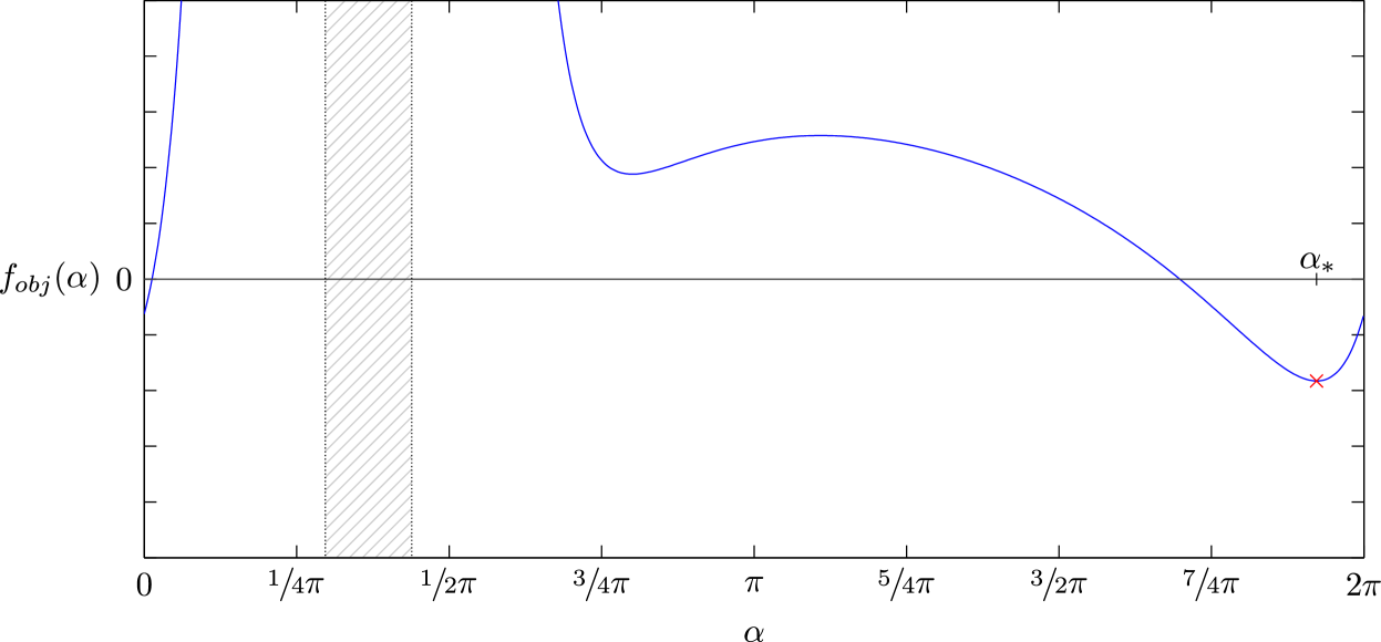
Figure 3: The objective function $f_{obj}$ is plotted in solid blue. The non-feasible region is indicated by gray stripes. The poles are marked by dotted lines. The global minimum is marked by a red cross.

Figure 4: An exemplary contact problem, where ${\bf A}$, $\bm{b}$ and $\mu$ are such that the conic section is a hyperbola and the objective function $f_{obj}$ has two local minima, but only one global minimum. Only the global minimum is dissipative.

Fig. 4 illustrates the optimization problem for an exemplary (dynamic) contact. Fig. 4 plots the quadratic objective function for points $\bm{x}_{to}$ on the plane of maximum compression and overlays the conic section. Fig. 4 plots the corresponding non-linear objective function $f_{obj}$ in comparison. An iterative approach for solving this constrained minimization problem that is guaranteed to converge linearly is derived in preclik14 (20). In the following an analytic approach is presented.

Let

be the unit vector tangential to the curve, where

Angles minimizing $f_{obj}$ must satisfy

$$\bm{t}(\alpha)^{\mathrm{T}}({\bf\hat{A}}\bm{\gamma}(\alpha)-\bm{\hat{b}})=0.$$ (7)

Insertion, trigonometric identity transformations and multiplication by $\frac{\mu^{2}b_{n}^{2}}{\overline{r}(\alpha)^{3}}$ leads to a trigonometric equation in the form of

$$c_{0}+c_{1}\cos(\alpha+\varphi_{1})+c_{2}\cos(2\alpha+\varphi_{2})=0,$$ (8)

with constants $c_{0},c_{1},c_{2},\varphi_{1},\varphi_{2}\in\mathbb{R}$ as specified in appendix A. The trigonometric equation can be transformed into a quartic equation by substituting $y=e^{i\alpha}=\cos\alpha+i\sin\alpha$. After solving the quartic equation for $y_{i}$, the corresponding angles $\alpha_{i}=\operatorname{atan2}(\operatorname{Im}(y_{i}),\operatorname{Re}(y_{i}))$ have to be checked for validity. Angles $\alpha_{i}\not\in 2\pi\mathbb{N}+\mathcal{I}$ are invalid as well as angles not satisfying Eq. (7) or Eq. (8) for that matter. Among all other candidates, the one with minimum objective function value amounts to the $2\pi$-periodic solution $\alpha_{*}$. Finally,

$$\bm{x}_{*}=\begin{pmatrix}A_{nn}^{-1}(b_{n}-A_{nt}\overline{r}(\alpha_{*})\cos\alpha_{*}-A_{no}\overline{r}(\alpha_{*})\sin\alpha_{*})\\ \bm{\gamma}(\alpha_{*})\end{pmatrix}.$$

Back to the case, where $b_{n}=0$ and $\mu>0$: If the conic section corresponds to a degenerate ellipse ($A_{nn}>\mu\sqrt{A_{nt}^{2}+A_{no}^{2}}$), then the solution is exactly this point. The conic sections that correspond to a degenerate parabola ($A_{nn}=\mu\sqrt{A_{nt}^{2}+A_{no}^{2}}$) are equivalent to the ray

$$\left\{r\begin{pmatrix}A_{nt}\\ A_{no}\end{pmatrix}\,\middle|\,r\in\mathbb{R}^{\geq 0}\right\}.$$

Degenerate hyperbolas correspond to the conical combination of two rays (along the asymptotes)

where $\alpha_{0}$ and $\Delta\alpha$ as in Eq. (6). Thus degenerate parabolas are a limiting case of degenerate hyperbolas with $\Delta\alpha=\pi$. Minimizing the energy over degenerate parabolas and hyperbolas can be implemented by checking, whether the unconstrained minimum $\bm{x}_{0}$ is contained in the friction cone. If that is not the case, then the objective function needs to be minimized along one of the rays:

The structogram in Fig. 5 summarizes the analytic solutions of the various cases involved in solving the single-contact problem.

$P_{1}=(x_{0,n}\geq 0\land\mathinner{\!\left\lVert\bm{x}_{0,to}\right\rVert}_{2}\leq\mu x_{0,n})\qquad P_{2}=(A_{nn}>\mu\sqrt{A_{nt}^{2}+A_{no}^{2}})$

Figure 5: The structogram describing the analytic solution of the single-contact problem.

4 Numerical Results

4.1 Academic Single-Contact Problem

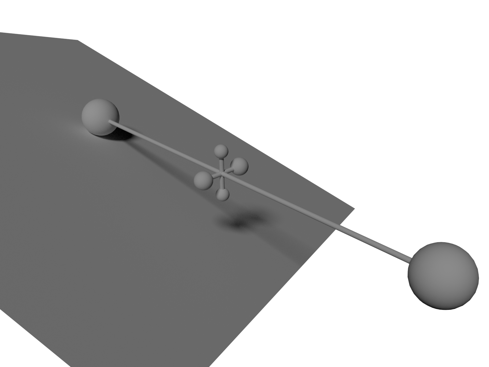
Figure 6: Illustration of the academic single-contact problem. An object constituted out of six point masses symbolized as spheres connected by massless rods collides with an inclined plane. The rods are aligned with the coordinate axis and the point masses are arranged symmetrically on each axis.

As an artificially constructed example consider a rigid body composed of six mass points connected by massless rods. The mass points are located symmetrically on the axes ($\pm d_{x}\bm{e}_{x},\pm d_{y}\bm{e}_{y},\pm d_{z}\bm{e}_{z}$) and both mass points on each axis concentrate the same mass ($m_{x},m_{y},m_{z}$). The center of mass thus coincides with the origin and the inertia tensor is given by

$${\bf I}=2\operatornamewithlimits{diag}(m_{y}d_{y}^{2}+m_{z}d_{z}^{2},m_{x}d_{x}^{2}+m_{z}d_{z}^{2},m_{x}d_{x}^{2}+m_{y}d_{y}^{2}).$$

Let the mass point in the positive x direction contact a plane with normal $\bm{n}$. Let $\bm{t}=\bm{n}\times\bm{e}_{x}$ and $\bm{o}=\bm{n}\times\bm{t}$ span the tangential plane. Let ${\bf Q}=\begin{bmatrix}\bm{n}\,\bm{t}\,\bm{o}\end{bmatrix}$ denote the contact frame. Then

$${\bf A}={\bf Q}^{\mathrm{T}}((2(m_{x}+m_{y}+m_{z}))^{-1}{\bf E}-d_{x}^{2}\bm{e}_{x}^{\times}{\bf I}^{-1}\bm{e}_{x}^{\times}){\bf Q}.$$

A rendering of this problem using $d_{x}=10$, $d_{y}=d_{z}=1$, $m_{x}=0.03$, $m_{y}=65$, $m_{z}=50$, $\mu=3.7$, $\bm{\hat{n}}=(0.25,0.36,-0.9)^{\mathrm{T}}$, $\bm{n}=\nicefrac{{\bm{\hat{n}}}}{{\mathinner{\!\left\lVert\bm{\hat{n}}\right\rVert}_{2}}}$ and $\bm{b}={\bf Q}^{\mathrm{T}}(0.06,0.7,0.23)^{\mathrm{T}}$ is shown in Fig. 6. The Coulomb solutions can be calculated for example using the polynomial root-finding approach described in bonnefon11 (3). The contact problem has three dynamic Coulomb solutions $\bm{x}_{i}$ ($i\in\{1,2,3\}$) directly opposing the post-impulse relative contact velocity in the tangential plane and a unique maximally dissipative solution $\bm{x}_{*}$. Approximate numerical values are listed in Tab. 1 for reference.

$\approx\bm{x}_{i}^{\mathrm{T}}$	$\approx({\bf A}\bm{x}_{i}-\bm{b})^{\mathrm{T}}$	$\approx\frac{1}{2}\bm{x}_{i}^{\mathrm{T}}{\bf A}\bm{x}_{i}-\bm{x}_{i}^{\mathrm{T}}\bm{b}$
$\begin{pmatrix}0.12&-0.44&-0.065\end{pmatrix}$	$\begin{pmatrix}0&0.40&0.060\end{pmatrix}$	$-0.252$
$\begin{pmatrix}0.29&-0.89&-0.62\end{pmatrix}$	$\begin{pmatrix}0&0.082&0.057\end{pmatrix}$	$-0.393$
$\begin{pmatrix}1.56&-0.99&-5.7\end{pmatrix}$	$\begin{pmatrix}0&0.0061&0.035\end{pmatrix}$	$-0.631$
$\approx\bm{x}_{*}^{\mathrm{T}}$	$\approx({\bf A}\bm{x}_{*}-\bm{b})^{\mathrm{T}}$	$\approx\frac{1}{2}\bm{x}_{*}^{\mathrm{T}}{\bf A}\bm{x}_{*}-\bm{x}_{*}^{\mathrm{T}}\bm{b}$
$\begin{pmatrix}1.6&-1.1&-5.8\end{pmatrix}$	$\begin{pmatrix}0&-0.057&0.034\end{pmatrix}$	$-0.634$

Table 1: Approximate Coulomb solutions and maximally dissipative solution for the numerically constructed single-contact problem including relative contact velocities in the contact frame and objective function values.

Fig. 7 plots the contour lines of the objective function for points in the plane of maximum compression and the boundary of the constraint set in solid blue. The red cross marks the maximally dissipative solution along the ellipse. The red circles mark the three Coulomb solutions.

Figure 7: Illustration of the academic contact problem including contour lines of the objective function, constraint set and solutions.

4.2 Paradox Single-Contact Problem

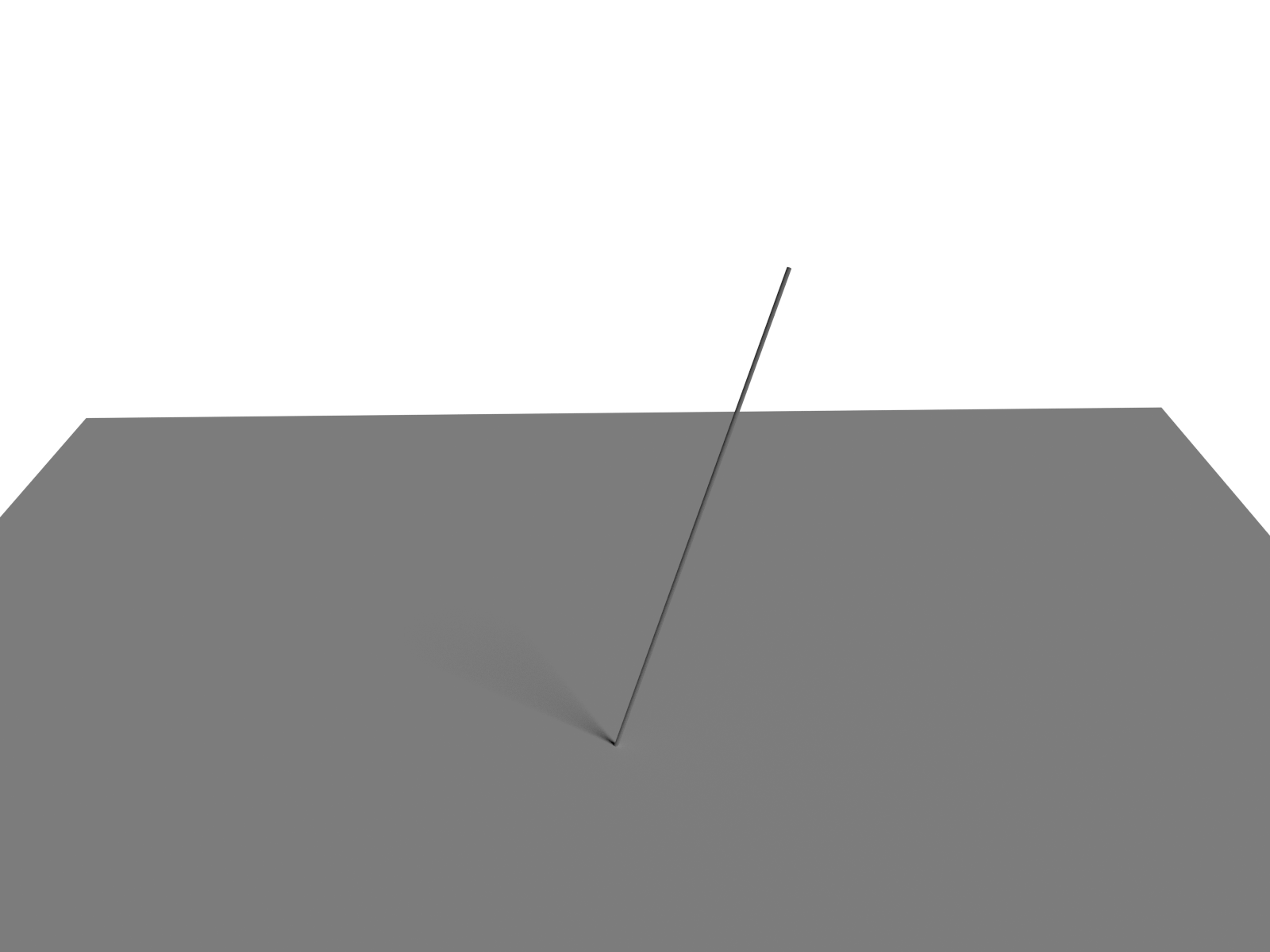
Figure 8: Illustration of the paradox single-contact problem. A slender rod is grazing along a plane.

Let a contact exist at time $t_{0}$ between a slender rod of length $l\in\mathbb{R}^{>0}$ and a half-space $\left\{\bm{x}\in\mathbb{R}^{3}\,\middle|\,\bm{n}^{\mathrm{T}}\bm{x}\leq 0\right\}$ with normal $\bm{n}=\bm{e}_{y}$. Let $\bm{t}=\bm{e}_{x}$ and $\bm{o}=\bm{e}_{z}$ complete the contact frame, where $\begin{bmatrix}\bm{e}_{x}&\bm{e}_{y}&\bm{e}_{z}\end{bmatrix}={\bf E}_{3}$. Let $0<\theta(t_{0})=\theta_{0}<\frac{\pi}{2}$ denote the initial angle between the plane and the rod. Let the slender rod correspond to rigid body $a$ and let the half-space correspond to rigid body $b$. The half-space is stationary such that $\bm{v}_{b}(t)=\bm{\omega}_{b}(t)=\bm{0}$, $m_{b}=\infty$ and ${\bf I}_{b}=\infty{\bf E}_{3}$. The rod shall be centered at the origin and aligned along the x axis of the body frame. Then, with uniformly distributed mass $m_{a}$, its body-frame inertia tensor is ${\bf I}_{a,0}=\frac{ml^{2}}{12}\operatornamewithlimits{diag}(\infty,1,1)^{\mathrm{T}}$. The rod is located in the x-y plane $\left\{\bm{x}\in\mathbb{R}^{3}\,\middle|\,\bm{e}_{z}^{\mathrm{T}}\bm{x}=0\right\}$ of the inertial frame with its center of mass at $\bm{x}_{a}(t_{0})=\frac{l}{2}(\cos\theta_{0},\sin\theta_{0},0)^{\mathrm{T}}$, such that the contact is closed initially ($\xi(t_{0})=0$). Let $\bm{\omega}_{a}^{-}(t_{0})=\bm{0}$ and $\bm{v}_{a}^{-}(t_{0})=-\bm{e}_{x}v_{0}$ with $v_{0}\in\mathbb{R}^{>0}$, such that initially the contact neither separates nor collides ($\dot{\xi}^{-}(t_{0})={{{\delta v}_{n}^{-}}}(t_{0})=0$). Let the contact position function $\bm{\hat{x}}$ track the lower tip of the slender rod. Let gravity $\bm{g}=-\bm{e}_{y}g_{0}$ with $g_{0}\in\mathbb{R}^{>0}$ act. A visualization of this setup is displayed in Fig. 8. Under these conditions the contact problem is essentially planar and corresponds to the paradox configuration published by Painlevé painleve1895 (18, 26).

If $t_{0}$ is a non-impulsive point in time ($t_{0}\not\in\mathcal{T}_{q}$), $\dot{\xi}^{-}(t_{0})=\dot{\xi}^{+}(t_{0})$ and since $\xi(t_{0})=\dot{\xi}^{\nicefrac{{-}}{{+}}}(t_{0})=0$, the acceleration-level non-penetration constraint is enabled from Fig. 1, where

$$\begin{split}\ddot{\xi}^{\nicefrac{{-}}{{+}}}(t_{0})&={{\dot{\delta v}_{n}^{\nicefrac{{-}}{{+}}}}}(t_{0})\ \text{and}\\ {{\dot{\bm{\delta v}}^{\nicefrac{{-}}{{+}}}}}(t_{0})&={\dot{\bm{v}}_{a}^{\nicefrac{{-}}{{+}}}}(t_{0})+{\dot{\bm{\omega}}_{a}^{\nicefrac{{-}}{{+}}}}(t_{0})\times(\bm{\hat{x}}(t_{0})-\bm{x}_{a}(t_{0}))\\ &+\bm{\omega}_{a}^{\nicefrac{{-}}{{+}}}(t_{0})\times(\bm{\omega}_{a}^{\nicefrac{{-}}{{+}}}(t_{0})\times(\bm{\hat{x}}(t_{0})-\bm{x}_{a}(t_{0})))\\ &={\bf W}(t_{0})^{\mathrm{T}}\begin{pmatrix}{\dot{\bm{v}}_{a}^{\nicefrac{{-}}{{+}}}}(t_{0})\\ {\dot{\bm{\omega}}_{a}^{\nicefrac{{-}}{{+}}}}(t_{0})\end{pmatrix}\\ &={\bf W}(t_{0})^{\mathrm{T}}{\bf M}(\bm{\varphi}(t_{0}))^{-1}{\bf W}(t_{0})\bm{\lambda}(t_{0})+\bm{g}.\end{split}$$

Since the contact is sliding at time $t_{0}$, the frictional contact reaction force is known to be

$$\bm{\lambda}_{to}(t_{0})=-\mu{{\lambda}_{n}}(t_{0})\frac{{\bm{\delta v}_{to}^{\nicefrac{{-}}{{+}}}}(t_{0})}{\mathinner{\!\left\lVert{\bm{\delta v}_{to}^{\nicefrac{{-}}{{+}}}}(t_{0})\right\rVert}_{2}}=\mu{{\lambda}_{n}}(t_{0})\begin{pmatrix}1\\ 0\end{pmatrix}.$$

Consequently,

$$\bm{\lambda}(t_{0})=\begin{bmatrix}\bm{n}&\bm{t}&\bm{o}\end{bmatrix}\begin{pmatrix}{{\lambda}_{n}}(t_{0})\\ \mu{{\lambda}_{n}}(t_{0})\\ 0\end{pmatrix}=\begin{pmatrix}\mu\\ 1\\ 0\end{pmatrix}{{\lambda}_{n}}(t_{0}).$$

Since gravity acts, the acceleration-level non-penetration constraint is compelled to be active. Thus,

$${{\dot{\delta v}_{n}^{\nicefrac{{-}}{{+}}}}}(t_{0})=\bm{n}^{\mathrm{T}}{\bf A}(t_{0})\begin{pmatrix}\mu\\ 1\\ 0\end{pmatrix}{{\lambda}_{n}}(t_{0})-g_{0}=0,\ {{\lambda}_{n}}(t_{0})\geq 0,$$

where ${\bf A}(t_{0})$ is given by Eq. (2):

The coefficient is then

The equation is not solvable for non-negative ${{\lambda}_{n}}(t_{0})$ if the coefficient is negative. The sign of the coefficient depends on $\mu$ and $\theta_{0}$. Thus, for a given angle $0<\theta_{0}<\frac{\pi}{2}$ the contact problem at hand has a non-impulsive solution if

$$\mu<\mu_{*}(\theta_{0})=\frac{\cos\theta_{0}+\frac{1}{3\cos\theta_{0}}}{\sin\theta_{0}},$$

where the lowest bound on $\mu$ is $\frac{4}{3}$ at the angle $\frac{1}{2}\cos^{-1}\left(-\frac{3}{5}\right)$. If this condition is not met, the assumption that $t_{0}$ is a non-impulsive point in time is wrong. Instead an impact problem has to be solved beforehand.

The impact model with purely inelastic impacts and Coulomb-like friction as presented in Fig. 1 exhibits multiple solutions. The zero solution $\bm{\Lambda}(t_{0})=\bm{0}$ is perfectly valid, since no collision is taking place ($\xi(t_{0})=\dot{\xi}^{-}(t_{0})=0$). However, it clearly does not lead to a post-impact state with a non-impulsive solution.

Any other solution must be located on the plane of maximum compression ($\dot{\xi}(t_{0})=0$) and in the friction cone. The impulse necessary to obtain a post-impulse sticking contact state is determined by the vector equation ${\bm{\delta v}^{+}}(t_{0})={\bf A}(t_{0})\bm{\Lambda}_{0}+\bm{v}_{a}^{-}(t_{0})=\bm{0}$:

It is easily verified, that $\bm{\Lambda}_{0}$ resides within the friction cone for any $0<\theta_{0}<\frac{\pi}{2}$ and any coefficient of friction requiring an impulsive solution ($\mu\geq\mu_{*}(\theta_{0})$):

$$\begin{split}\mathinner{\!\left\lVert\bm{\Lambda}_{0,to}\right\rVert}_{2}&=\frac{m_{a}v_{0}}{8}(5+3\cos(2\theta_{0}))\\ &=\mu_{*}(\theta_{0})\frac{m_{a}v_{0}}{8}3\sin(2\theta_{0})\\ &\leq\mu\frac{m_{a}v_{0}}{8}3\sin(2\theta_{0})=\mu{{\Lambda}_{0,n}}.\end{split}$$

Thus $\bm{\Lambda}(t_{0})=\bm{\Lambda}_{0}$ is a second solution of the impact problem effecting a slip-stick transition. In fact, there also can be an infinite number of sliding solutions. For example in the edge case where $\mu=\mu_{*}(\theta_{0})$, all convex combinations of the $\bm{0}$ solution and the $\bm{\Lambda}_{0}$ solution are also solutions, where the slip directly opposes the frictional impulse.

When replacing the impact model with the Coulomb-like friction by the impact model complying with the maximum dissipation principle, the structogram in Fig. 5 easily identifies the unique impulsive solution: If $\mu\geq\mu_{*}(\theta_{0})$, then $\bm{\Lambda}(t_{0})=\bm{\Lambda}_{0}$. It is the same impulsive solution as the sticking solution in the impact model with the Coulomb-like friction. Conversely, if a non-impulsive solution exists ($\mu<\mu_{*}(\theta_{0})$), then $\bm{\Lambda}_{0}$ is not contained in the friction cone and predicate $P_{2}$ in the structogram then always selects $\bm{\Lambda}(t_{0})=\bm{0}$:

$$\begin{split}A_{nn}&=1+3\cos^{2}\theta_{0}=\mu_{*}(\theta_{0})3\sin\theta_{0}\cos\theta_{0}\\ &>\mu 3\sin\theta_{0}\cos\theta_{0}=\mu\sqrt{A_{nt}^{2}+A_{no}^{2}}.\end{split}$$

Thus the impact problem results in the zero solution if a non-impulsive solution exists as expected. The impact model with Coulomb-like friction behaves the same way in this respect: If $\mu<\mu_{*}(\theta_{0})$ then the plane of maximum compression intersects the friction cone only at $\bm{0}$.

The impulsive contact reaction $\bm{\Lambda}(t_{0})=\bm{\Lambda}_{0}$ leads in both impact models to a sticking post-impulse contact state, where non-impulsive contact reactions exist for the subsequent contact problem. However, alternate solutions of the impact model with Coulomb-like friction do not necessarily lead to subsequent contact problems with non-impulsive solutions.

4.3 Macro-Scale Behaviour

The macro-scale behaviour of the proposed maximum dissipation friction model is compared to the Coulomb friction model by numerical simulations of fast granular channel flows. All simulations are carried out with the pe module of the waLBerla multi physics framework freely available at walberla.net. The algorithms are based on time stepping methods presented in Sec. 3. The parallel implementation is described in preclik14 (20, 21). For the computations the compute resources of the Regionales Rechenzentrum Erlangen (RRZE) are used. The Emmy cluster comprises 560 compute nodes, each equipped with two Xeon 2660v2 proccessors (10 cores, 2-way SMT) clocked at 2.2 GHz and 64 GiB of RAM.

Figure 9: Top-down view of the simulation area. The particle channel is confined by solid walls in y and z direction. A constant particle inflow at the left side is artificially created. Within the channel an obstacle is present to disturb the particle flow.

The simulation domain is a rectangular channel confined by solid walls in the y and z direction. Its dimensions are $$15\text{\,}\mathrm{c}\mathrm{m}$\times$6.5\text{\,}\mathrm{c}\mathrm{m}$\times$2.0\text{\,}\mathrm{c}\mathrm{m}$$. The channel is filled with monodisperse spherical particles with a diameter of $0.47\text{\,}\mathrm{m}\mathrm{m}$ and a density of $2.65\text{\,}\mathrm{g}\mathrm{/}\mathrm{c}\mathrm{m}^{3}$. These are arranged on a regular rectangular grid with a spacing of $1\text{\,}\mathrm{m}\mathrm{m}$. All particles are given an initial velocity of $1\text{\,}\mathrm{m}\mathrm{/}\mathrm{s}$ in positive x direction. A random perturbation velocity in y and z direction is applied with each component varying between $-0.5\text{\,}\mathrm{m}\mathrm{/}\mathrm{s}$ and $0.5\text{\,}\mathrm{m}\mathrm{/}\mathrm{s}$. To produce a steady inflow a moving plane with infinite mass is added at the left end of the channel ($x=$0\text{\,}\mathrm{c}\mathrm{m}$$). This plane moves with $1\text{\,}\mathrm{m}\mathrm{/}\mathrm{s}$ pushing the particles into the channel. After the plane has moved a distance equal to two times the radius of the particles the position of the plane is reset and a new layer of particles is generated. This process is repeated throughout the whole simulation generating an inflow rate of roughly $1.4\text{\cdot}{10}^{6}$ particles per second. The other end of the channel remains open and the particles leaving the channel are deleted. All the particles are also influenced by a gravitational acceleration of $9.81\text{\,}\mathrm{m}\mathrm{/}\mathrm{s}^{2}$ in negative z direction. In the region $[$3\text{\,}\mathrm{c}\mathrm{m}$,$5\text{\,}\mathrm{c}\mathrm{m}$]\times[$3\text{\,}\mathrm{c}\mathrm{m}$,$5\text{\,}\mathrm{c}\mathrm{m}$]\times[$0\text{\,}\mathrm{c}\mathrm{m}$,$2\text{\,}\mathrm{c}\mathrm{m}$]$ a stationary object obstructing the channel is introduced. The obstacle is composed of a cylinder with radius $1\text{\,}\mathrm{c}\mathrm{m}$ located at ($4\text{\,}\mathrm{c}\mathrm{m}$, $4\text{\,}\mathrm{c}\mathrm{m}$, $1\text{\,}\mathrm{c}\mathrm{m}$) with its axis aligned along the z axis. The right half of the cylinder is replaced by a box. A cross-section of this setup is sketched in Fig. 9.

For the computation the domain is decomposed into $16\times 10\times 4$ evenly sized rectangular subdomains. Each subdomain is handled by one process totaling to 640 processes which are distributed onto 32 nodes of the Emmy cluster. The time-step length is chosen to be $10\text{\,}\mathrm{\SIUnitSymbolMicro}\mathrm{s}$. This guarantees a stable simulation. The total simulation time is $10\text{\,}\mathrm{s}$ resulting in $1\text{\cdot}{10}^{6}$ time steps. After these time steps all initial perturbations are resolved. The implementation of the collision resolution solver described in preclik14 (20) is used. Both friction models use a coefficient of friction equal to $0.4$.

	Coulomb	Max. Dissipation
avg. number of particles	$246\,992.291\,708\,291\,7$	$247\,005.050\,949\,050\,96$
solid volume fraction	$57.2\text{\,}\mathrm{\char 37\relax}$	$57.2\text{\,}\mathrm{\char 37\relax}$
avg. number of contacts	$320\,276.507\,492\,507\,5$	$320\,196.819\,180\,819\,2$
avg. number of contacts per particle	$2.593\,412\,978\,820\,955$	$2.592\,633\,777\,734\,896$
max. penetration ($\mathrm{\SIUnitSymbolMicro}\mathrm{m}$)	$39.060\,022\,8$	$46.497\,616\,79$

Table 2: Key figures collected for both simulations. Samples were collected every $10\text{\,}\mathrm{m}\mathrm{s}$ during the $10\text{\,}\mathrm{s}$ total simulation time.

Some general information about the simulation is collected every 1000 time steps and averaged over the complete simulation. Within the range of accuracy both friction models result in almost identical values which are summarized in Tab. 2. The average number of particles in the simulation domain is $2.47\text{\cdot}{10}^{5}$ which leads to a solid volume fraction of $57.2\text{\,}\mathrm{\char 37\relax}$. During every time step an average of $3.20\text{\cdot}{10}^{5}$ contacts which equals $2.59$ contacts per particle are resolved. The maximum penetration depth between two particles was $39.060\,022\,8\text{\,}\mathrm{\SIUnitSymbolMicro}\mathrm{m}$ ($8.31\text{\,}\mathrm{\char 37\relax}$ of the particle radius) in the Coulomb friction case and $46.497\,616\,79\text{\,}\mathrm{\SIUnitSymbolMicro}\mathrm{m}$ ($9.89\text{\,}\mathrm{\char 37\relax}$ of the particle radius) in the maximum dissipation case.

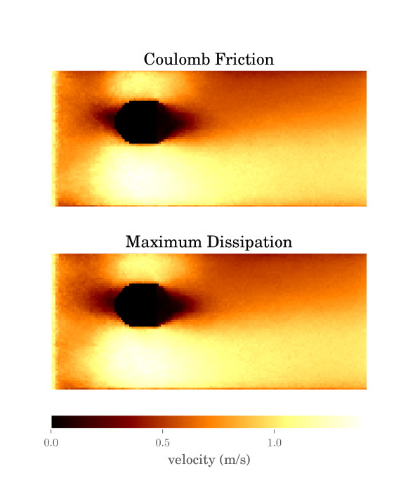
Figure 10: Velocity profile of the particles throughout the channel. Around the obstacle the velocity of the particles increases due to the narrowing of the channel. After the obstacle collisions as well as friction slow down the fast particles again.

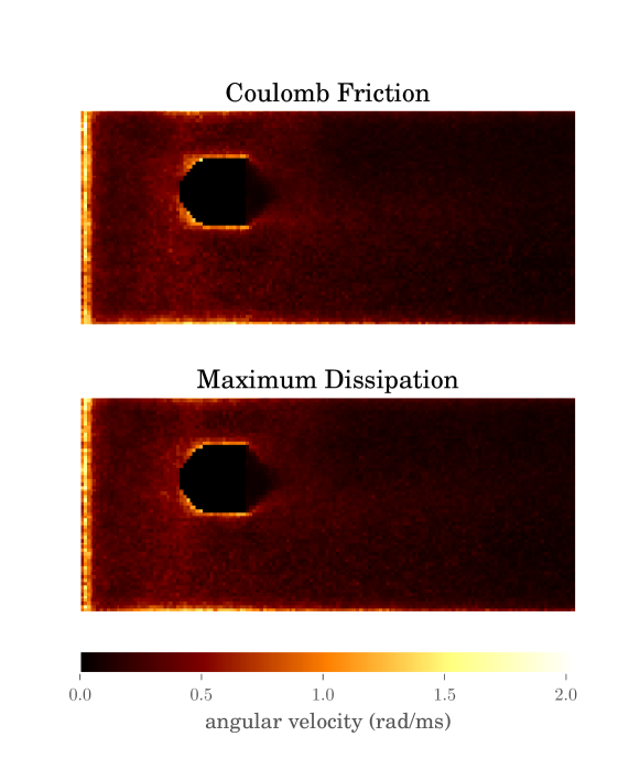
Figure 11: Angular velocity profile of the particles throughout the channel. One can see that rotations do not play a major role in this setup as friction damps any angular velocity rapidly. A certain amount of rotating particles can be found at the inflow and near the stationary object in the middle of the channel.

To validate the accordance of both friction models the last frame of each simulation is used and the particle configuration is analyzed. The particles are sorted into $$150$\times$65$$ equally sized cells in the x-y plane ignoring the z axis and the velocity (see Fig. 10) as well as the angular velocity (see Fig. 11) is averaged over all particles within one cell. Both simulations show a very similar velocity profile throughout the whole channel. The particles right after the inflow have very high velocities but are damped rapidly. After a short almost homogeneous region the particles gain speed again as the channel narrows around the obstacle. The particle velocities peak at $1.42\text{\,}\mathrm{m}\mathrm{/}\mathrm{s}$ (Coulomb Friction) and $1.39\text{\,}\mathrm{m}\mathrm{/}\mathrm{s}$ (Maximum Dissipation) respectively. The angular velocity comparison shows a similar picture. After a short initial region the angular velocity gets damped heavily. At the boundary of the stationary obstacle and the walls, the angular velocity stays high due to friction. Both friction models result visually in a similar behaviour.

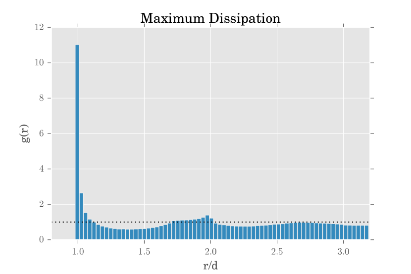
Figure 12: Radial distribution function of the particles near the outflow. The radial distance $r$ is given in units of the particle diameter $d=$0.47\text{\,}\mathrm{m}\mathrm{m}$$. The dotted line $g(r)=1$ represents the value for a completely amorphous material.

As a last check the radial distribution function of the particles near the exit is analyzed to obtain insight into the spatial arrangement. The region $[$12\text{\,}\mathrm{c}\mathrm{m}$,$14\text{\,}\mathrm{c}\mathrm{m}$]\times[$0\text{\,}\mathrm{c}\mathrm{m}$,$6.5\text{\,}\mathrm{c}\mathrm{m}$]\times[$0\text{\,}\mathrm{c}\mathrm{m}$,$2\text{\,}\mathrm{c}\mathrm{m}$]$ is chosen. All the inter-particle distances are calculated and summed up in a histogram. The histogram is then normalized by the total number of particles and the expected amount of particles within each individual bin - $\int_{x_{0}}^{x_{1}}4\pi\rho r^{2}\text{d}r$, with $\rho$ being the overall particle density and $x_{0}$, $x_{1}$ being the boundaries of the corresponding histogram bin. For both friction models the histogram can be found in Fig. 12. They match almost exactly. One can see a strong peak at a distance equal to the particle diameter which indicates a dense packing. The rest of the histogram does not reveal additional favored distances suggesting an amorphous packing.

The numerical experiment described above shows no significant difference between the two friction models. The newly developed maximum dissipation friction model thus reproduces the expected macro scale behaviour.

5 Summary

In this paper, an alternative purely inelastic frictional impact model is presented. In that impact model the contact reaction impulses consistently maximize dissipation leading to unique contact reactions for single-contact impact problems. An academic single-contact impact problem is analyzed, demonstrating the potential non-uniqueness of the impulsive contact reactions if Coulomb-like friction constraints act instead. Furthermore, a paradox single-contact impact problem was analyzed. It was found that the impact model maximizing dissipation results in the solution producing a slip-stick transition, whereas the impact model with Coulomb-like friction in addition allows the zero solution and possibly even an infinite number of dynamic solutions, which not necessarily result in configurations with subsequent non-impulsive solutions. The paper also shows how the impact model based on the maximum dissipation principle can be embedded in an impulse-velocity time-stepping scheme. A numerical experiment is conducted to demonstrate that changing from an impact model with Coulomb-like friction to the maximally dissipative impact model in the time-stepping scheme has a negligible influence on the macroscopic behaviour of a granular channel flow past an obstacle. The multi-contact problem is solved using a blend between a non-linear block Gauss-Seidel and a weighted non-linear block Jacobi, where each block corresponds to a single-contact problem. The paper presents an analytic solution of the single-contact problem that can act as a subsystem solver in the non-linear block relaxation method. The analytic solution involves transforming the single-contact problem into a quartic equation with complex coefficients. Back transformation and filtering of the solutions of the quartic equation leads to the unique contact reaction maximizing dissipation. Additionally, the analytic solution can be used to resolve two-particle collisions in event-driven integrations of rigid-body dynamics.

The presented impact model is missing a restitution hypothesis for partly elastic impacts. Even though applying Poisson’s hypothesis is straightforward, the extension of the impact model by an energetically consistent restitution hypothesis is not. Also proving or falsifying that the constructed time-stepping scheme converges to a solution of the corresponding integral equations remains an open problem. Besides addressing the non-uniqueness in the impact model, the approach might also be transferable to remove non-uniqueness in the non-compliant contact model when non-penetration and friction constraints on the acceleration-level are enabled.

Appendix A Appendix

$c_{0}=$

$\frac{3}{2}\mu A_{nn}(A_{no}b_{t}-A_{nt}b_{o})$

$c_{1}=$

$(\mu^{4}((A_{no}^{2}(A_{tt}^{2}+A_{to}^{2})-2A_{nt}A_{no}A_{to}\allowbreak(A_{tt}+A_{oo})+A_{nt}^{2}(A_{to}^{2}+A_{oo}^{2}))b_{n}^{2}+2(A_{nt}b_{o}-A_{no}b_{t})(A_{no}^{2}A_{to}+A_{nt}\allowbreak A_{no}\allowbreak(A_{tt}-A_{oo})-A_{nt}^{2}A_{to})b_{n}+(A_{nt}^{2}+A_{no}^{2})(A_{nt}b_{o}-A_{no}b_{t})^{2})\allowbreak+2\mu^{2}A_{nn}\allowbreak((2A_{nt}A_{no}A_{to}-A_{no}^{2}A_{tt}-A_{nt}^{2}A_{oo})\allowbreak b_{n}^{2}+A_{nn}\allowbreak(A_{no}\allowbreak(A_{tt}b_{o}-A_{to}b_{t})-A_{nt}\allowbreak(A_{to}b_{o}-A_{oo}b_{t}))b_{n}+A_{nn}\allowbreak(A_{nt}b_{o}-A_{no}b_{t})^{2})+A_{nn}^{2}((A_{nt}^{2}+A_{no}^{2})b_{n}^{2}-2A_{nn}\allowbreak(A_{nt}b_{t}+A_{no}b_{o})b_{n}+A_{nn}^{2}(b_{t}^{2}+b_{o}^{2})))^{\nicefrac{{1}}{{2}}}$

$c_{2}=$

$\mu A_{nn}\allowbreak((\frac{1}{4}\allowbreak(A_{tt}^{2}+A_{oo}^{2})+A_{to}^{2}-\frac{1}{2}A_{tt}A_{oo})b_{n}^{2}+(A_{no}\allowbreak(\frac{1}{2}\allowbreak(A_{tt}-A_{oo})b_{o}-A_{to}b_{t})-A_{nt}\allowbreak(A_{to}b_{o}+\frac{1}{2}\allowbreak(A_{tt}-A_{oo})b_{t}))\allowbreak b_{n}+\frac{1}{4}\allowbreak((A_{nt}^{2}+A_{no}^{2})b_{o}^{2}+(A_{nt}^{2}+A_{no}^{2})b_{t}^{2}))^{\nicefrac{{1}}{{2}}}$

$\varphi_{1}=$

$\operatorname{atan2}(\mu^{2}((A_{no}A_{to}-A_{nt}A_{oo})b_{n}-A_{no}^{2}b_{t}+A_{nt}A_{no}\allowbreak b_{o})-A_{nn}^{2}b_{t}+A_{nn}A_{nt}b_{n},\allowbreak\mu^{2}((A_{nt}A_{to}-A_{no}A_{tt})b_{n}+A_{nt}A_{no}b_{t}-A_{nt}^{2}b_{o})-A_{nn}^{2}b_{o}+A_{nn}A_{no}b_{n})$

$\varphi_{2}=$

$\operatorname{atan2}((A_{tt}-A_{oo})b_{n}-A_{nt}b_{t}+A_{no}b_{o},\allowbreak 2A_{to}b_{n}-A_{no}\allowbreak b_{t}-A_{nt}b_{o})$

References

• (1) M. Anitescu and F.A. Potra “Formulating Dynamic Multi-Rigid-Body Contact Problems with Friction as Solvable Linear Complementarity Problems” In Nonlinear Dynamics 14.3 Springer, 1997, pp. 231–247
• (2) Marcus N Bannerman, Robert Sargant and Leo Lue “DynamO: A free O(N) general event-driven molecular dynamics simulator” In Journal of computational chemistry 32.15 Wiley Online Library, 2011, pp. 3329–3338
• (3) O. Bonnefon and G. Daviet “Quartic Formulation of Coulomb 3D Frictional Contact”, 2011
• (4) J. Diebel “Representing Attitude: Euler Angles, Unit Quaternions, and Rotation Vectors”, 2006
• (5) K. Erleben “Stable, Robust, and Versatile Multibody Dynamics Animation”, 2004
• (6) Bogdan I Gavrea, Mihai Anitescu and Florian A Potra “Convergence of a class of semi-implicit time-stepping schemes for nonsmooth rigid multibody dynamics” In SIAM Journal on Optimization 19.2 SIAM, 2008, pp. 969–1001
• (7) A. Hassanpour et al. “Analysis of Particle Motion in a Paddle Mixer using Discrete Element Method (DEM)” In Powder Technology 206.1 Elsevier, 2011, pp. 189–194
• (8) C.T. Jayasundara et al. “CFD–DEM Modelling of Particle Flow in IsaMills – Comparison Between Simulations and PEPT Measurements” In Minerals Engineering 24.3 Elsevier, 2011, pp. 181–187
• (9) Michel Jean “The non-smooth contact dynamics method” In Computer methods in applied mechanics and engineering 177.3 Elsevier, 1999, pp. 235–257
• (10) Yan-Bin Jia “Three-dimensional impact: energy-based modeling of tangential compliance” In The International Journal of Robotics Research 32.1 SAGE Publications Sage UK: London, England, 2013, pp. 56–83
• (11) Yan-Bin Jia and Feifei Wang “Analysis and Computation of Two Body Impact in Three Dimensions” In Journal of Computational and Nonlinear Dynamics, 2016
• (12) B. Mirtich “Impulse-based Dynamic Simulation of Rigid Body Systems”, 1996
• (13) Brian Mirtich and John Canny “Impulse-based simulation of rigid bodies” In Proceedings of the 1995 symposium on Interactive 3D graphics, 1995, pp. 181–ff ACM
• (14) B.K. Mishra and R.K. Rajamani “The Discrete Element Method for the Simulation of Ball Mills” In Applied Mathematical Modelling 16.11 Elsevier, 1992, pp. 598–604
• (15) N. Mitarai and H. Nakanishi “Granular Flow: Dry and Wet” In The European Physical Journal Special Topics 204.1 Springer, 2012, pp. 5–17
• (16) J. J. Moreau “Unilateral Contact and Dry Friction in Finite Freedom Dynamics” In Nonsmooth Mechanics and Applications Springer Vienna, 1988, pp. 1–82
• (17) A.M. Al-Fahed Nuseirat and G.E. Stavroulakis “A complementarity problem formulation of the frictional grasping problem” In Computational Methods in Applied Mechanics and Engineering, 2000
• (18) P. Painlevé “Sur les lois du frottement de glissement” In C. R. Acad. Sci. Paris 121, 1895, pp. 112–115
• (19) Constantin Popa, Tobias Preclik and Ulrich Rüde “Regularized solution of LCP problems with application to rigid body dynamics” In Numerical Algorithms 69.1 Springer, 2015, pp. 145–156
• (20) Tobias Preclik “Models and Algorithms for Ultrascale Simulations of Non-smooth Granular Dynamics”, 2014
• (21) Tobias Preclik and Ulrich Rüde “Ultrascale simulations of non-smooth granular dynamics” In Computational Particle Mechanics 2.2 Springer, 2015, pp. 173–196
• (22) J. Sauer and E. Schömer “A Constraint-Based Approach to Rigid Body Dynamics for Virtual Reality Applications” In Proceedings of the ACM Symposium on Virtual Reality Software and Technology, 1998, pp. 153–162
• (23) Yunian Shen and WJ Stronge “Painlevé paradox during oblique impact with friction” In European Journal of Mechanics-A/Solids 30.4 Elsevier, 2011, pp. 457–467
• (24) David E Stewart “Convergence of a Time-Stepping Scheme for Rigid-Body Dynamics and Resolution of Painlevé’s Problem” In Archive for Rational Mechanics and Analysis 145.3 Springer, 1998, pp. 215–260
• (25) David E Stewart “Dynamics with Inequalities: impacts and hard constraints” SIAM, 2011
• (26) D.E. Stewart “Rigid-Body Dynamics with Friction and Impact” In SIAM review 42.1 Society for IndustrialApplied Mathematics, 2000, pp. 3–39
• (27) D.E. Stewart and J.C. Trinkle “An Implicit Time-Stepping Scheme for Rigid Body Dynamics with Inelastic Collisions and Coulomb Friction” In International Journal of Numerical Methods in Engineering 39.15 Wiley Online Library, 1996, pp. 2673–2691
• (28) William J Stronge “Rigid body collisions with friction” In Proceedings of the Royal Society of London A: Mathematical, Physical and Engineering Sciences 431.1881, 1990, pp. 169–181 The Royal Society
• (29) William James Stronge “Impact mechanics” Cambridge university press, 2004
• (30) A. Tasora and M. Anitescu “A Convex Complementarity Approach for Simulating Large Granular Flows” In Journal of Computational and Nonlinear Dynamics 5.3 American Society of Mechanical Engineers, 2010, pp. 1–10
• (31) Alessandro Tasora and Mihai Anitescu “A matrix-free cone complementarity approach for solving large-scale, nonsmooth, rigid body dynamics” In Computer Methods in Applied Mechanics and Engineering 200.5 Elsevier, 2011, pp. 439–453