On the assessment of the nature of open star clusters and the determination of their basic parameters with limited data

Abstract

Our knowledge of stellar evolution and of the structure and chemical evolution of the Galactic disk largely builds on the study of open star clusters. Because of their crucial role in these relevant topics, large homogeneous catalogues of open cluster parameters are highly desirable. Although efforts have been made to develop automatic tools to analyse large numbers of clusters, the results obtained so far vary from study to study, and sometimes are very contradictory when compared to dedicated studies of individual clusters. In this work we highlight the common causes of these discrepancies for some open clusters, and show that at present dedicated studies yield a much better assessment of the nature of star clusters, even in the absence of ideal data-sets. We make use of deep, wide-field, multi-colour photometry to discuss the nature of six strategically selected open star clusters: Trumpler 22, Lynga 6, Hogg 19, Hogg 21, Pismis 10 and Pismis 14. We have precisely derived their basic parameters by means of a combination of star counts and photometric diagrams. Trumpler 22 and Lynga 6 are included in our study because they are widely known, and thus provided a check of our data and methodology. The remaining four clusters are very poorly known, and their available parameters have been obtained using automatic tools only. Our results are in some cases in severe disagreement with those from automatic surveys.

Keywords open clusters: general — open clusters: individual (Trumpler 22, Lynga 6, Hogg 19, Hogg 21, Pismis 10, Pismis 14)

1 Introduction

In the last decade many attempts have been made to obtain basic parameters for large sets of open star clusters (e.g. Kharchenko et al. 2005, 2013; Bukowiecki et al. 2011; Glushkova et al. 2010; Loktin et al. 2001; Tadross 2011). The goals of these studies are obvious: first to provide large samples of clusters with homogeneous fundamental parameters, and, second, eventually to use these samples to probe the properties of the Galactic thin disk, where most open clusters reside, and/or of the open cluster population as a whole. Some of these studies are limited to membership and parameter determination (e.g. Kharchenko et al. 2013; Caetano et al. 2015), while other explore properties of the disk (Popova & Loktin 2005, 2008; Tadross 2014) or of the open cluster population as a whole (Buckner & Froebrich 2014; Kharchenko et al. 2016, and references therein).

In general, these studies extract the necessary data from public surveys – mostly the 2MASS (Skrutskie et al. 2006) archive – and use automatic star counts and quick inspection of photometric diagrams to decide about the nature of a cluster, and then derive its parameters in a semi-automatic way, with different degrees of sophistication (Krone-Martins & Moitinho 2014, Caetano et al. 2015). The most popular of these catalogues is that from Kharchenko al. (2005, 2013), which also provides proper motions, but the data are usually limited to the brightest stars. A through-full and critical comparison of the results coming out of these different data-sets has recently been provided by Netopil et al. (2015).

Briefly, typical limitations of these works are: (1) the evaluation of the clusters’ reality is based on just a handful of stars, (2) there is a general lack of a proper error assessment (which is reflected by the artificially high precision of the parameter estimates), (3) a systematic neglecting of previous investigations, leading to gross mistakes in many cases, and (4) in many instances the plots used to infer clusters’ properties are very difficult to read. Large discrepancies among different compilations are often found (Netopil et al. 2015), and one is led to the frustrating conclusion that the large number of star clusters in a compilation does not compensate for the poor and quick analysis of the individual objects. As we shall discuss here, a through-full data analysis is unavoidable, and should focus on two crucial aspects: a careful visual inspection of the clusters surface density and photometric diagrams, and an exhaustive and critical literature search.

It is well known that a truly complete analysis of a star cluster is extremely difficult: astrometric, photometric, and spectroscopic data need to be acquired and analysed (see e.g. Curtis et al. 2013, Costa et al. 2015, and references therein). In most cases only photometry is available. Nevertheless, if photometry covers the whole cluster area, it is sufficiently deep, and it is multi-colour, it may be possible to reach solid conclusions about the physical nature of a group of stars, by means of well-known, powerful, classical procedures. The results can obviously be strengthened and refined later by incorporating spectroscopic and kinematic studies.

In this work, we have selected a strategic sample of open clusters to illustrate how to obtain solid estimates of the basic parameters of a star cluster based on limited data, and to highlight the common limitations of automatic surveys. We present deep, wide field, multicolor (UBVI_kc) photometry and star counts for 6 clusters: Trumpler 22, Lynga 6, Hogg 19, Hogg 21, Pismis 10 and Pismis 14. Trumpler 22 and Lynga 6 are relatively well studied objects, and provided the means to check our data and methodology. The former was included to illustrate an easy case, while the latter is clearly a more complicated one because of the large reddening value. We obtained new data for Hogg 19, for which only VI data was available, and for which serious discrepancies are present in the literature. We also present new data for Hogg 21, Pismis 10 and Pismis 14, for which only semi-automatic parameter estimates are available from Kharchenko et al. (2013). In Table 1 we present the coordinates of our targets.

The layout of the paper is as follows. In Section 2 we present a careful scan of the available literature on the clusters of interest, and in Section 3 we discuss the observations and the reduction procedure; in Section 4 we concisely describe our data analysis strategy, while in Section 5 we explain with some detail the methodology used for the star counts. In Section 6 the full analysis of the various photometric diagrams is presented. Finally, in Section 7 we summarise our findings.

2 Literature overview

Trumpler 22

Lindoff(1968) obtained UBV photographic photometry and concluded that the cluster is 100 Myr old and is located at a distance of 1700 pc, for a reddening of E(B-V) = 0.51. Previous distance estimates were based on a smaller number of stars, and resulted in larger distances: 1800 pc (Barkhatova 1950), 2210 pc (Trumpler 1930) and 2500 pc (Collinder 1931). Similarly, estimates of the radius have resulted in a wide range of sizes: 7 arcmin (Trumpler 1930), 8 arcmin Lindoff (1968), 10 arcmin (Collinder 1931) and 23 arcimn (Barkhatova 1950).

The nature of Trumpler 22 as a physical star cluster has been questioned by Haug (1978). Based on photographic material he concluded that Trumpler 22 is a spurious agglomeration. On the contrary, de La Fuente Marcos & de La Fuente Marcos (2009) suggested that Trumpler 22 forms a primordial pair with the nearby star cluster NGC 5617. Recently, this latter possibility was scrutinised in detail by De Silva et al. (2015) by using CCD UBVI photometry and and high resolution spectroscopy. They concluded that Trumpler 22 is indeed a real cluster, and that its fundamental parameters (age, distance and metallicity) do agree with those of NGC 5671, thus supporting the earlier suggestion that they form a binary cluster system. Their proposed parameters are: an age of 70 Myr, a reddening E(B-V) =0.48 and a distance of 2100 pc. For this cluster Kharchenko et al (2013) do provide a reddening consistent with other studies (0.50), but obtained the smallest distance (1614 pc) and the oldest age (250 Myr).

Lynga 6

This is another example of a well studied object that has not always been considered a physical group. It is famous mostly because it most probably hosts the Cepheid TW Normae. Moffat & Vogt (1975) could not reach firm conclusions about the cluster’s nature because of their shallow photometry. Madore (1975) obtained a distance of 2500 pc, for a reddening of E(B-V) = 1.35. The first CCD study is that from Walker (1985), who suggests that the cluster is 100 Myr old, and is located at 2000 pc for a reddening of E(B-V) = 1.34. Hoyle et al. (2003) highlights the difficulties to determine the cluster parameters due to significant differential reddening. This difficulty can be handled more easily in the infrared, as Majaess et al. (2011) demonstrated. They derived an age of 80 Myr and a distance of 1.9$\pm$0.1 kpc, for a reddening E(J-K) = 0.38$\pm$0.02. For this cluster Kharchenko et al (2013) provide a reddening E(B-V) = 1.27, the smallest distance (1771 pc) and the youngest age ($\sim$ 30 Myr).

Hogg 19

Seleznev et al. (2010) provide the only dedicated study available for this cluster. Their analysis of CCD VI and 2MASS JHK photometry suggests that Hogg 19 might be as old as 2.5 Gyr, and at a distance of 2.6 kpc, for a reddening of E(B-V) = 0.65. Bukowiecki et al. (2011) using 2MASS photometry suggest an age of 1.3 Gyr, a reddening E(B-V)=0.60, and a distance of 3266 pc. Kharchenko et al. (2013), using the vary same 2MASS data obtained different values for the basic parameters: a distance of 898 pc, a reddening E(B-V) = 0.416, and an age slightly above 1.0 Gyr. The two studies rely on very different approaches to derive the cluster parameters, and therefore Hogg 19 stands out as a particularly crucial test-case for the present study.

Hogg 21

The only parameter determination available for this cluster is that from the large survey of Kharchenko et al. (2013), who suggest the following solution: an age of 28.1 Myr, a distance of 1750 pc, and a reddening E(B-V) = 0.729.

Pismis 10

The only parameter determination available for this cluster is that from the large survey of Kharchenko et al. (2013), who suggest the following solution: an age of 251.2 Myr, a distance of 8835 pc, and a reddening E(B-V) = 1.457

Pismis 14

The only parameter determinations available for this cluster are those from the large survey of Kharchenko et al. (2013), who suggest the following solution: an age of 223.8 Myr, a distance of 1775 pc, and a reddening E(B-V) = 0.479, and from Bukowiecki et al. (2011), who suggest the following solution: 22 Myr for the age, 0.56 for E(B-V) , and a distance of 1314 pc.

3 Observations and data reduction

The observations were carried out with the Y4KCAM camera attached to the Cerro Tololo Inter-American Observatory (CTIO, Chile) 1-m telescope, operated by the SMARTS consortium . This camera is equipped with an STA $4064\times 4064$ CCD detector, with 15-$\mu$m pixels, yielding a scale of 0.289^′′/pixel and a field-of-view (FOV) of $20^{\prime}\times 20^{\prime}$ at the Cassegrain focus of the telescope. This FOV is large enough to cover the whole clusters and to sample the surrounding Galactic field. This is shown in Fig. 1 where we provide V-band CCD images for the six fields.

All observations were carried out in photometric, good-seeing conditions. Our UBVI instrumental photometric system was defined by the use of a standard broad-band Kitt Peak UBVI_kc set of filters. To determine the transformation from our instrumental system to the standard Johnson-Kron-Cousins system, and to correct for extinction, each night we observed Landolt’s areas PG 1047 and SA 98 (Landolt 1992) multiple times, and with a wide range of air-masses. Field SA 98 in particular includes over 40 well-observed standard stars, with a good magnitude and color coverage: $9.5\leq V\leq 15.8$, $-0.2\leq(B-V)\leq 2.2$, $-0.3\leq(U-B)\leq 2.1$. In Table 2 we present the log of our observations.

Basic calibration of the CCD frames was done using the Yale/SMARTS y4k reduction script based on the IRAF package ccdred, and the photometry was performed using IRAF’s daophot and photcal packages. Instrumental magnitudes were extracted following the point spread function (PSF) method (Stetson 1987) using a quadratic, spatially variable master PSF (gaussian function). Finally, the PSF photometry was aperture corrected using 25 bright, not saturated, isolated stars across the whole field.

The aperture photometry was carried out using the PHOTCAL package and we used transformation equations of the form:

u = U + u1 + u2 $\times$(U-B) + u3 $\times$X (1)
b = B + b1 + b2 $\times$(B-V) + b3 $\times$ X (2)
v = V + v1_bv + v2_bv $\times$ (B-V) + v3_bv $\times$X (3)
v = V + v1_vi + v2_vi $\times$ (V-I) + v3_vi $\times$X (4)
i = I_kc + i1 + i2 $\times$ (V-I) + i3 $\times$ X (5)

where UBVI_kc and $ubvi$ are standard and instrumental magnitudes respectively, and X is the airmass of the observation. Subscripts 1 clearly refer to zero points, and 2 to color terms. We adopted as mean values for the extinction coefficients (subscripts 3) the typical values of the CTIO site (see Baume et al. 2009).

To derive V magnitudes, we used Eq. 3 when the B magnitude was available; otherwise we used Eq. 4. The calibration coefficients and their uncertainties are shown in Table 3. In Fig. 2 the reader can appreciate the trend of global (PSF plus calibration) photometric errors (specifically for Trumpler 22), and notice that they are well below 0.05 mag down to V$\sim$19.5 for all color combinations.

World Coordinate System (WCS) header information of each frame was obtained using the ALADIN tool and 2MASS data (Skrutskie et al. 2006). This procedure allows us to obtain a reliable astrometric calibration ($\sim 0.12^{\prime\prime})$ and is explained in full details in Baume et al. (2009).

We used the STILTS tool to manipulate tables and cross-correlate our $UBVI_{kc}$ with the $JHK$ 2MASS data. We thus obtained a catalogue with astrometric/photometric information for all detected objects in a FOV of approximately $20^{\prime}\times 20^{\prime}$ of each cluster region (see Fig. 1). The full catalogues are made available in electronic form at the CDS website.

As a sanity check of our photometry, we compared our data for Trumpler 22 with that of De Silva et al. (2015), which was obtained with a different telescope and CCD detector. From a grand-total of 1572 stars in common we obtained, in the sense of ours minus theirs:

$\Delta$ V = 0.03$\pm$0.08,
$\Delta$ (B-V) = 0.03$\pm$0.07,
$\Delta$ (U-B) = -0.06$\pm$0.11, and
$\Delta$ (V-I) = 0.02$\pm$0.10.

Fig. 3 illustrates the nice agreement between the two data sets.

4 Methodology

We briefly summarise our methodology here. The interested readers can found a more detailed description in Carraro & Seleznev (2012).

By definition, a Galactic cluster is a density enhancement above the general Galactic field. Therefore, the first step is to define this over-density using star counts and estimate its radius. To this end, we follow Seleznev (2016), where the procedure is fully described. It should be noted however, that an over-density is only a good indication of the possible existence of a cluster, but not a proof of the reality of a physical entity. In the Galactic disk, in many occasions over-densities are generated by random fluctuations in extinction across the field of view and by chance alignments (Carraro 2006, and references therein). Therefore, a close inspection of photometric diagrams -the classical two color diagram (TCD) and colour-magnitude diagram- (CMD), is mandatory to check whether the stars generating the over density also produce well defined photometric sequences.

For this latter purpose we make extensive use of the U filter, and apply the Q-method, as described in Hiltner & Johnson (1956). This method allows us to identify stars sharing common reddening properties, and derive their individual reddening, via comparison with a zero reddening, zero age main sequence (ZAMS). In this study we adopt the ZAMS defined originally by Turner (1976, 1979), and later validated by Turner & Burke (2002) and Turner (2010).

Once corrected for reddening, stars are plotted in the reddening corrected CMD, where their distance is estimated using the very same ZAMS, which is displaced only vertically to fit the star distribution. This fit is normally done both in the $V_{o}/(B-V)_{o}$ and $V_{o}/(U-B)_{o}$ diagram, to ensure a simultaneous solid fit. Finally, age is derived on the same diagrams employing solar metallicity isochrones from the Padova suite of models (Bressan et al. 2012), that we adopt here for consistency with our previous studies (see, e.g. Carraro & Seleznev 2012). This latter study also describes how the errors of the basic parameters are estimated.

In this study we refrain from complementing our photometric material with astrometric data. Any attempt we made resulted in confused vector point diagrams. We ascribe this negative result to the crowding of our fields, and to the presence in many cases of high and patchy extinction.

5 Star counts

The surface density maps for our program clusters (see Fig. 4) were derived with the use of a kernel estimator (Silverman 1986). We have used this method several times in the past (see e.g. Carraro & Seleznev 2012; Carraro et al. 2016), and we refer the reader to Seleznev (2016) for an exhaustive description of it. These maps were derived using a kernel halfwidth ($h$) of 3 arcmin. Different density values are shown with different shades in Fig. 4. Their numerical values are indicated in the shade scales. Axes show the distance from the center of the field in arcmin. The positive direction of the Y axis coincides with the direction to the North, while the positive direction of the X axis coincides with the direction to the East. Star counts were also limited to an area one $h$ away from the detector borders, to avoid under-sampling effects.

Together with other basic cluster parameters, our results on the clusters geometry are given in Table 4. Columns 3 and 4 give the center coordinates determined by us: RA and DEC for 2000.0 equinox, in degrees, and column 5 gives our estimated cluster radius in arcmin. The second column in the table shows the $V$ limiting magnitude ($V_{lim}$) that was adopted in each case to construct the surface density map. This limiting magnitude was determined analysing the density maps at varying $V_{lim}$ in combination with a visual inspection of the CMD of each cluster.

Each cluster centre was determined as a coordinates of maximum points of the corresponding linear densities also plotted by the kernel estimator method (Seleznev et al. 2017). The centre of an open cluster is not a well-defined value. It depends on limiting magnitude, the kernel halfwidth, the spectral band. In the present work the limiting magnitudes were used as indicated in Table 4. The kernel halfwidth for the linear densitiy was selected taking into account the density profiles for sample clusters. The general condition for the cluster centre coordinates was the density profile without a non-physical minimum at the centre of the clusters.

Using the clusters center coordinates previously obtained, radial density profiles were then derived, again using the kernel estimator method. These profiles are shown in Fig. 5. The vertical axis is the surface density in units of $arcmin^{-2}$. The horizontal axis represents the distance from the cluster center in arcminutes. As before, profiles are limited to a region one $h$ away from the detector border (which corresponds to about one arcmin). Density profiles are shown with a thick solid lines, and the areas depicting the 2$\sigma$–width confidence intervals are shown with dotted lines. These intervals were obtained by means of a smoothed bootstrap estimate method (Seleznev 2016).

We have also made visual estimates of the background stellar density, which are indicated with thin solid lines. These were determined as follows.

If the density profile exhibits an approximately flat area above the horizontal axis limit, then the background density line is drawn taking into account the approximate equality of the square of areas between this line and the density profile above and below it. The cluster radius is then estimated as the abscissa of of the intersection of the density profile and the background density line. The corresponding uncertainty is then the distance from the abscissa of the point of intersection of the confidence interval line with the background density line at the cluster radius location. This was the case for Hogg 21, Lynga 6, Pismis 10, and Trumpler 22, suggesting that these clusters might have an extended halo, and thus the FOV investigated might not be large enough. In such cases it is more conservative to consider these radii as lower estimates.
If the density profile does not show a flat area and decreases up to the limit of the horizontal axis, then only an upper limit of the background density value can be estimated. In these cases, obviously, only a lower limit of the cluster size can be inferred.

6 Photometric diagram analysis

In this section we deal with the interpretation of photometric diagrams constructed taking into account our results from the star counts. They are mostly CMDs, but in some cases we also employ TCDs in the $B-V/U-B$ plane to support our conclusions.

6.1 Trumpler 22

This well studied cluster was included among our targets as a sanity check of our photometry, and to ensure that our method is producing reliable and reproducible results. This cluster stands out as a significant density enhancement above the general Galactic field (see Fig 4, bottom right panel), and we estimate its radius as 6.4$\pm$0.5 arcmin (see Fig. 5 and Table 4). Its center is slightly off-set with respect to nominal published coordinates (see Table 1). In Fig 6 we show our parameter solution. In the left panel we show the reddening derivation, done using a ZAMS. It was found to be E(B-V) =0.48$\pm$0.03. The uncertainty was obtained by displacing the ZAMS back and forth along the reddening vector direction until a fit was not possible anymore. Using the Q-method we corrected all stars for their individual reddening, and thus derived a reddening corrected CMD, which is shown in the right panel (only for the brightest stars). The red solid line is the same ZAMS as in the left panel, displaced vertically by (m-M)_o=11.4$\pm$0.2. This implies a distance of 1.9${}^{+0.2}_{-0.1}$, in excellent agreement with De Silva et al. (2015). The black solid isochrone, taken from Bressan et al. (2012), is for an age of 70 Myr, and does provide a nice fit to the distribution of stars seen in the CMD. Our age estimation is in agreement with De Silva et al. (2015) as well.

6.2 Lynga 6

Basic parameters available for this cluster are considered quite solid. The infrared study by Majaess et al. (2011) dealt successfully with the uncertainties in reddening and distance that affected previous optical CCD photometry (Hoyle et al 2003), produced by the high and variable extinction in the FOV towards the cluster. Our star counts analysis highlights a significant over-density at the cluster position (see Fig. 4 mid-left panel), and implies a radius of 5.5$\pm$0.3 arcmin for Lynga 6. Stars selected within this distance from the cluster center were used to construct the CMDs shown in Fig. 7 for three different color combinations. There is a main sequence (MS) significantly wide in color because of variable reddening. An experienced eye can also identify an interesting feature, namely a bifurcation of the MS at $V\sim 16$ and $(B-V)\sim 1.2$, $(V-I)\sim 1.5$, and $(B-I)\sim 2.5$, which further widens the upper MS. We argue that Lynga 6 lies in the red side of the sequence, while the blue side is simply the continuation of the field star sequence.

In Fig. 8 we present our parameter solution for Lynga 6. In the upper left panel we show a TCD, where we plot a ZAMS to fit the distribution of the reddest stars, that we recognised in the CMD. This ZAMS has been displaced by $E(B-V)$ = 1.25. We then derived stars’ individual reddening using the Q-method, and their distribution is shown in the upper right panel. This distribution peaks at $E(B-V)$ = 1.2$\pm$0.1, which lends further support to our previous guess of the cluster reality and location in the CMD. In the lower panel we present a reddening corrected CMD, from which we have estimated distance and age. Beyond any doubt, stars sharing a common reddening produce a distinctive feature at a distance of 2.0${}^{+0.1}_{-0.1}$ kpc, as implied by the vertical shift of (m-M)_o = 11.5$\pm$0.1 needed to fit the data with a ZAMS (red solid line). This is in excellent agreement with the infrared study of Majaess et al. (2011). The black isochrone (displaced by the same amount in absolute distance modulus) is for an age of 79 Myr, again in excellent agreement with Majaess et al. (2011). For this cluster, the parameter estimates provided by Kharchenko et al. (2013) are in agreement with ours, with the exception of their age, which is half our value.

6.3 Hogg 19

CMDs for this cluster are presented in Fig. 9. In these diagrams, we only included stars inside the cluster radius (see Table 4), and for which the uncertainty in the $V$ magnitude is smaller than 0.02 mag (see Fig. 2). The only evident features are a well populated MS, and a tilted clump of stars at V $\sim$15 stretched in the direction of the reddening vector (see Carraro & Costa 2009, or Baume et al 2009, for very similar occurrences). At first glance we cannot recognise any obvious turn off point (TO).

The left and middle panels show CMDs in the $V/B-V$ and $V/V-I$ planes, respectively. The right panel shows the same CMD as in the middle panel, but with two solar metallicity isochrones (Bressan et al. 2012) superimposed; an improved parameter solution close to the one by Seleznev et al. (2010, in red), and the other for that of Kharchenko et al. (2013, in blue). To make the solutions comparable, we transformed Kharchenko et al. (2013) reddening from E(B-V) into E(V-I), using E(V-I) = 1.244$\times$ E(B-V). The solution in red adopts E(V-I)=1.0, which provides a better fit than in Seleznev et al. (2010), and relies on the fact that the red clump might indicate the existence of an old star cluster, for which the main sequence turnoff (TO) would be located at $V\sim 18.7$, $(B-V)\sim 1.3$. This TO seems to correspond to a thick blue MS, which appears on top of the general distribution of stars. This sequence has a different shape than the sequence brighter than $V$=18.7, and at this magnitude level one can appreciate a significant change in the density of stars. The blue solution, on the other hand, is in general quite a poor fit. It seems to rely on the existence of a clump of only two stars, and on the assumption that the TO coincides roughly with the brightest stars. If correct, it implies that Hogg 19 is a twin of the nearby star cluster NGC 6134, which has fundamental parameters very similar to the ones of this fit.

Clearly, little more can be extracted from these CMDs alone. The two solutions can be seen as equally valid, and therefore a closer scrutiny is necessary. We decided therefore to adopt a different strategy, and make use of the $U$-band data. In Fig. 10 we present a classical TCD in the $B-V/U-B$ plane, which is well known to be very effective to identify common reddening early spectral type stars, and to separate populations with different reddening. The solid black line is ZAMS, that we include for reference, together with the direction of the reddening, indicated by an arrow in the top-right corner of the diagram. In spite of the scattering, two groups can clearly be identified: one with very low reddening, composed of stars of spectral type A0 and later, and most probably located close to the Sun; and a second group, affected by larger reddening (0.7$\pm$0.1) -and hence more distant- with stars of spectral type as early as B5, which we fit with the blue ZAMS. We tentatively associate this latter group with the Carina-Sagittarius arm (see below). In this TCD we see no trace of a population with $E(B-V)\sim 0.4$. This evidence excludes Kharchenko et al. (2013) solution. There is no trace of stars as faint as the Hogg 19 MS which would support the suggestion by Seleznev et al. (2010). This is because the U photometry is not deep enough. In fact the TO in this case is too shallow, and for its (B-V) color there are only very few stars having also a measure in (U-B) (see Fig. 9 and 10).

To further discriminate between the above two possibilities, we resorted to star counts and produced surface density maps for the stars in the two magnitude regions that better highlight each solution (from the right panel of Fig. 9 ). The results are shown in Fig. 11. The left panel represents stars brighter than $V$=14 (and E(B-V)$\sim$0.4, see above), which should produce evidences supporting the suggestion by Kharchenko et al. (2013). Although there is a sort of elongated concentration above and to the right, of the center of the field, the density contrast is so low that we can safely conclude that the distribution of bright stars across the field is homogeneous. We suggest this sparse group is made of interlopers, namely a few young stars located in the intervening Carina-Sagittarius spiral arm.

On the other hand, the right panel shows the density map for stars in the magnitude range $18\leq V\leq 20$, which would belong to the TO of Hogg 19, according to Seleznev et al. (2010). In this case the density contrast is much higher, and although the structure of the concentration is irregular, a peak is clearly visible.

These evidences altogether lend support Seleznev et al. (2010) suggestion, that we revised here . Kharchenko et al. (2013) could not detect the cluster because of the shallowness of their photometry, and ended up confusing it with a sparse group of young stars belonging to the intervening Carina Sagittarius arm (see Carraro et al. 2010 for a similar concurrence).

6.4 Hogg 21

This cluster presents an easier case compared to Hogg 19. It stands as a low contrast over density in the top-right panel of Fig. 4. The CMD in Fig. 12 shows two distinct features: a thick sequence with a TO at V$\sim$ 17, and a scattered group of blue stars brighter than $V\sim 15$. For this latter group one can guess a TO at $V\sim 13$. In a TCD constructed with the stars within the cluster radius (see left panel of Fig. 13), a clear sequence of young star appears, reddened by E(B-V) = 0.48$\pm$0.02, as indicated by the red ZAMS. At odds with Hogg 19, the sequence of young stars is much less scattered, and corresponds to a spatially confined structure, enhancing the probability that we are facing a physical cluster and not a random distribution of young stars. Using the Q method, we derived stars’ individual reddening, and plotted the early type stars in the reddening-corrected CMD shown in the right panel of Fig 13, from which a distance modulus of $(m-M)_{o}$=11.65$\pm$0.10 is implied. Some scatter is clearly visible, but we ascribe it to the presence of binary stars, and to photometric errors, particularly in the $(U-B)$ color index. This distance modulus places Hogg 21 at 2.1${}^{+0.1}_{-0.1}$ kpc from the Sun. The isochrone super-imposed in the figure is for an age of 100 Myr, which we inferred from the earliest spectral type stars present in the cluster; i.e., about B6 (see also the TCD). Our estimates of the cluster distance and age do not differ much from those of Kharchenko et al. (2013), but reddening does, meaning that the apparent distance modulus from Kharchenko (2013) is clearly off. We note that significant systematic offsets in the reddening estimates of Kharchenko et al. (2013) have been already reported in the literature (see, e.g., Buckner & Froebrich 2014, 2016; Netopil et al. 2015).

6.5 Pismis 10

The surface density map for the FOV in the direction to Pismis 10, shown in the mid-right panel of Fig. 4, indicates a mild, wide, over density. However, a quick look at Fig. 1 (or any DSS map) suggests that this over density might be a reddening effect, since the surrounding region is highly obscured. The CMDs presented in Fig. 14 hardly indicate any distinctive feature in any of the color combinations, but the TCD for stars inside the cluster radius (see Fig. 5 and Table 4) presented in the left panel in Fig. 15 shows a group of extremely and differentially reddened stars, which might constitute an obscured star cluster, in full similarity with Lynga 6. The reddening solution for this group is in fact $E(B-V)$=1.5$\pm$0.1. After correcting these stars for individual reddening, they distribute in the reddening corrected CMD ( right panel of Fig. 15) in a cluster of $\sim$ 250 Myr, at a distance of less than 2.7${}^{+0.3}_{-0.2}$ kpc [(m-M)_o=12.2$\pm$0.2]. In this case, our age and reddening are close to Kharchenko et al. (2013). Their distance estimate however differs by a very large amount. Again, this is caused by the insufficient depth of their photometry.

6.6 Pismis 14

On maps this cluster appears as a shallow over density a few arcmin from the more conspicuous open cluster NGC 2910 (Giorgi et al. 2015), from which it is separated by a clear dust lane (see the bottom-left panels of Figs. 1 and 4, or any DSS image). As such, Pismis 14 might simply constitute a random enhancement of a few bright stars, or, possibly, be part of the outer corona of NGC 2910. The CMDs presented in Fig. 16 illustrate this latter possibility. When considering stars outside the estimated radius of Pismis 14, a MS is clearly visible, which would belong to NGC 2910 (right panel). On the contrary, the stars inside the cluster region (left panel) do not show any distinctive feature.

The TCD for all stars in the FOV of Pismis 14 in Fig. 17 indicates a group of early type stars, that must belong to NGC 2910. They are reddened by $E(B-V)$ = 0.20, in perfect agreement with the recent study of NGC 2910 by Giorgi et al. (2015). These authors as well stress the large differences between their cluster parameters and those determined by Kharchenko et al. (2013). Our conclusion is that Pismis 14 is a change alignment of a few bright stars enhanced by a patchy reddening distribution. These stars are probable peripheral members of NGC 2910.

7 Discussion and conclusions

We have presented and discussed multi-color CCD photometry of six Galactic open clusters: Trumpler 22, Lynga 6, Hogg 19, Hogg 21, Pismis 10, and Pismis 14. The main goal of the present study was to assess the nature of these clusters and derive their basic parameters: reddening, age, and distance. Comparison of our results with the literature has allowed us to highlight (and possibly explain) existing discrepancies with large semi-automatic parameter surveys, which stresses their present limitations.

Trumpler 22 and Lynga 6 are well studied stars clusters, and we have obtained results consistent with previous dedicated works. For Lynga 6, the extensive usage of U-band photometry allowed us to reproduce infrared results in a critical case of heavy reddening.

Hogg 19 revealed itself as an extremely challenging object, and previous studies have been vastly discrepant in their results (Kharchenko et al. 2013; Seleznev et al. 2010). A careful and synoptic analysis of both star counts and photometric diagrams show this is a $\sim$ 2 Gyr old cluster. This is quite an interesting results, given the general paucity of old clusters in the inner Galaxy (Carraro et al. 2014, Jacobson et al. 2016). In this case the cause of the discrepancy is twofold: first, the photometry used by Karchenko et al. (2013) is too shallow and they missed the real cluster; second, they did not take into account previous literature results.

We found that Hogg 21 is a young star cluster associated with the Carina Sagittarius arm. It is significantly less reddened than the estimate by Kharchenko et al. (2013). Systematic issues with their reddening estimates have been routinely reported in the literature (Buckner & Froebrich 2014; Netopil et al. 2015).

Pismis 10 attracted our attention because of the very large heliocentric distance ($\sim$ 9 kpc) reported by Kharchenko et al. (2013). This would place it well beyond the Vela Molecular Ridge (Carraro & Costa 2010; Giorgi et al. 2015) at the extreme periphery of the Galactic disk. We found that this cluster is very reddened, as Lynga 6, but lies much closer, at about 3 kpc from the Sun.

We finally provide evidences that Pismis 14 is not a physical cluster, but a chance alignment of a few bright stars member of the outer corona of the nearby cluster NGC 2910.

In closing, we acknowledge that efforts are being made by several groups (Caetano et al. 2015; Krone-Martins & Moitinho 2014; Netopil et al. 2015; Carraro et al. 2016, and references therein) to provide new tools, or re-discover old methods, to derive reliable open cluster parameters. Hopefully, the closed box era of open clusters’ fundamental parameter determination will be over soon. Along this vein, future Gaia mission data releases will surely be very valuable to ensure the homogeneity of star cluster fundamental parameters for all those clusters which will be at reach.

Acknowledgements G. Baume acknowledges financial support from the ESO visitor program that allowed a visit to ESO premises in Chile, where part of this work was done. G. Carraro science leave in Ekaterinburg (where most of this was was done) was supported by Act 211 Government of the Russian Federation, contract No. 02.A03.21.0006, and by the ESO DGDF program. E. Costa acknowledges support by the Fondo Nacional de Investigación Científica y Tecnológica (proyecto No. 1110100 Fondecyt) and the Chilean Centro de Excelencia en Astrofísica y Tecnologías Afines (PFB 06).

Facilities: CTIO SMARTS.

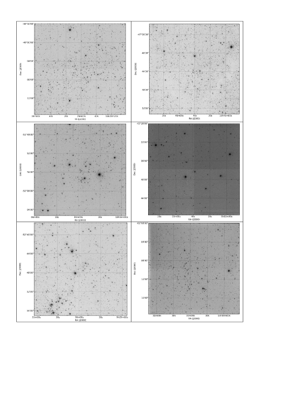
Fig. 1 : $V$-band CCD images of the fields observed. Top row: Hogg 19 and 21. Middle row: Lynga 6 and Pismis 10. Bottom row: Pismis 14 and Trumpler 22.

Fig. 2 : Global photometric errors as a function of $V$ magnitude for Trumpler 22.

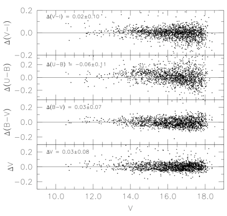
Fig. 3 : Comparison of our photometry for Trumpler 22 with that of De Silva et al. (2015), in the sense of our data minus theirs.

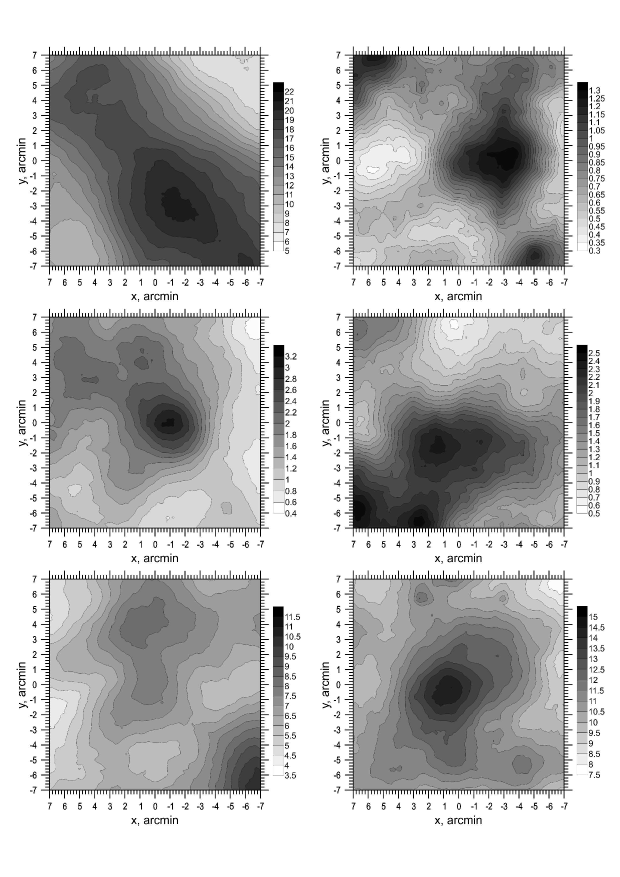
Fig. 4 : Surface density maps. From the top to bottom: Hogg 19 and Hogg 21, Lynga 6 and Pismis 10, Pismis 14 and Trumpler 22 .

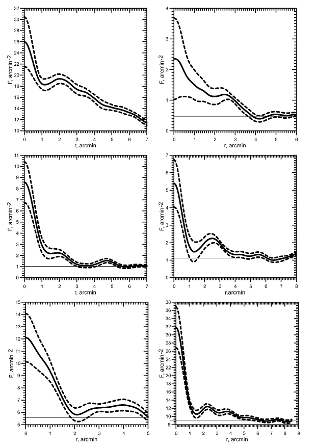
Fig. 5 : Radial density profiles. From top to bottom: Hogg 19 and Hogg 21, Lynga 6 and Pismis 10, Pismis 14 and Trumpler 22 .

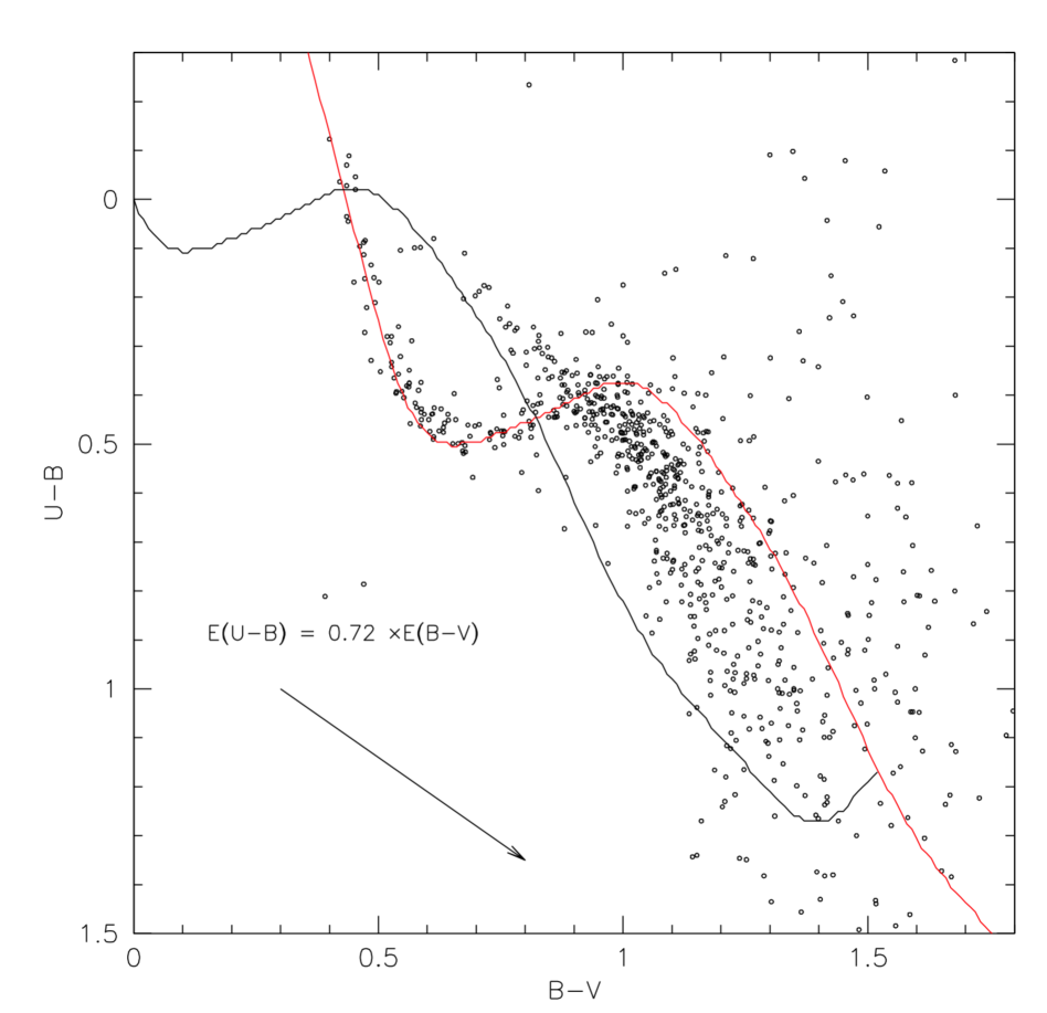
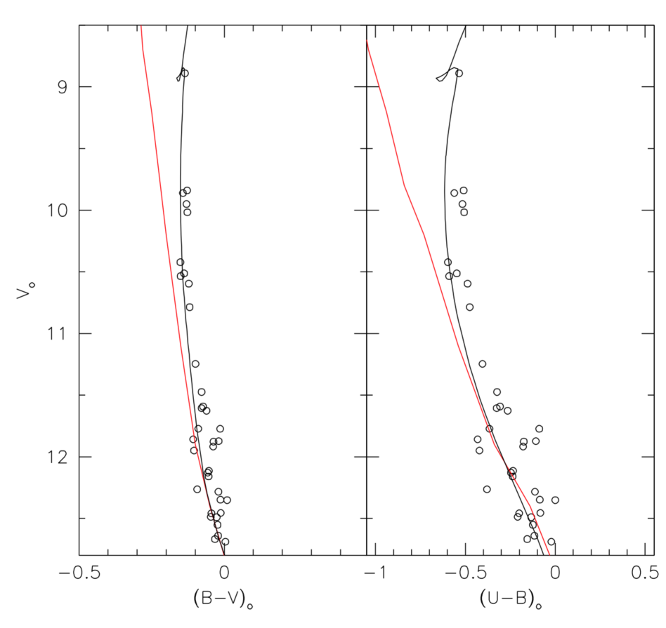
Fig. 6 : Parameter solution for Trumpler 22. The left panel shows the TCD, and the reddening solution. The solid black and red lines are ZAMS. The red ZAMS has been shifted by $E(B-V)=0.48$ in the direction of the reddening vector. The right panel shows the reddening corrected CMD used for our distance and age solution. The red line is a ZAMS displaced vertically by (m-M)_o=11.4; the black line is an isochrone for an age of 70 Myr.

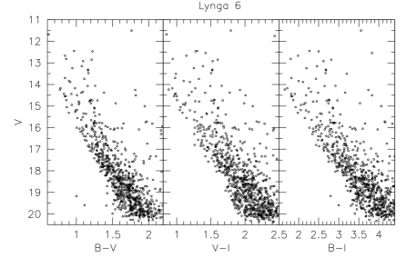
Fig. 7 : CMDs, in three different color combinations, for Lynga 6 stars located inside the cluster radius.

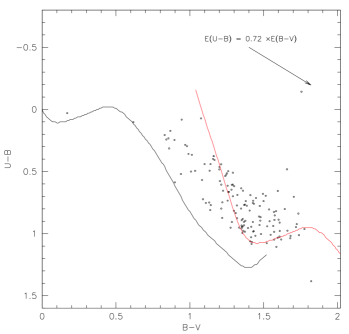
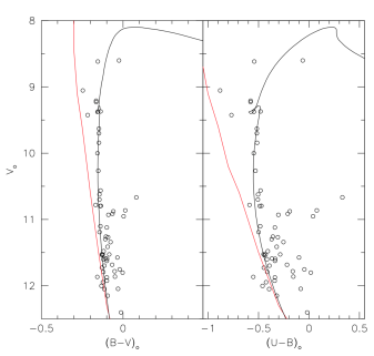
Fig. 8 : Parameter solution for Lynga 6. The upper left panel shows the TCD, where the red line is a ZAMS shifted by $E(B-V)=1.25$. The upper right panel illustrates the individual reddening distribution. The lower panel, finally, shows the distance and age solution. The red line is a ZAMS displaced vertically by (m-M)_o=11.5, and the black line is an isochrone for an age of 79 Myr.

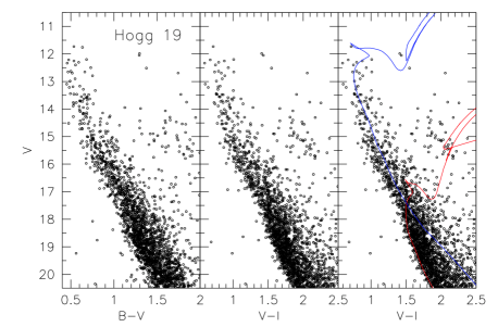
Fig. 9 : CMDs of Hogg 19 in $V/B-V$ (right panel) and $V/V-I$ (middle panel). In the right panel we included the parameter solutions from Kharchenko et al. (2013, in blue) and the one from this study (in red).

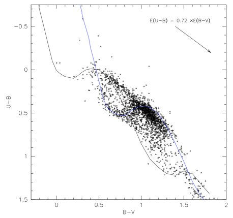
Fig. 10 : TCD diagram of Hogg 19. Only stars having $\sigma_{U,B,V}\leq 0.02$ are shown. See text for details.

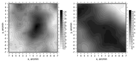
Fig. 11 : Surface density map for stars bright than $V=14$, which sample Hogg 19 according to Kharchenko et al. (2013) solution (left panel), and for stars fainter than $V=18$, to reproduce our solution.

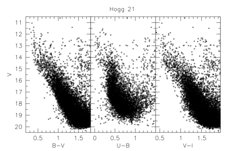
Fig. 12 : CMDs of Hogg 21 in $V/B-V$ (left panel), $V/U-B$ (middle panel), and $V/V-I$ (right panel).

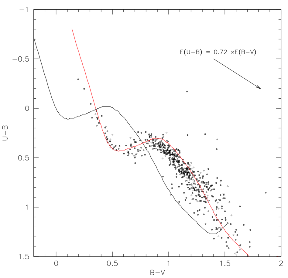
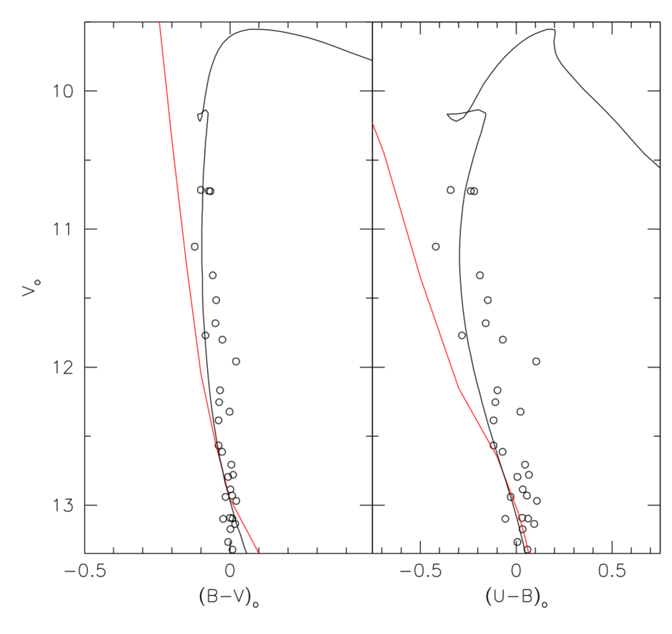
Fig. 13 : Left panel: TCD of Hogg 21, and reddening solution. Right panel: distance and age solution. See text for details,

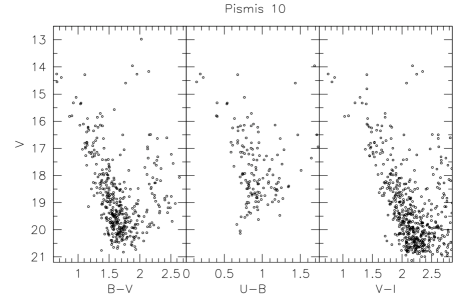
Fig. 14 : CMDs of Pismis 10 in $V/B-V$ (left panel), $V/U-B$ (middle panel), and $V/V-I$ (right panel).

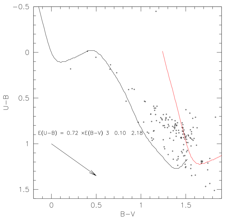
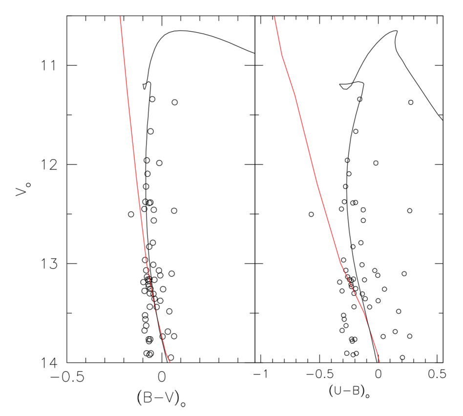
Fig. 15 : Left panel: TCD of Pismis 10, and reddening solution. Right panel: distance and age solution. See text for details.

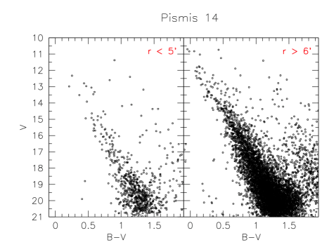
Fig. 16 : CMDs of Pismis 14 in $V/B-V$. Left panel: stars within the cluster estimated radius to exclude contamination from NGC 2910. Right panel: stars outside the cluster area, to highlight NGC 2910.

Fig. 17 : TCD of Pismis 14 and NGC 2910, and reddening solution for NGC 2910.

Table 1 : Stellar fields studied in this work

Cluster	RA(2000.0)	Dec (2000.0)	$l$	$b$
	[deg]	[deg]	[deg]	[deg]
Pismis 10	135.6500	-42.6330	265.429	1.960
Pismis 14	142.4625	-52.7833	275.150	-1.145
Trumpler 22	217.7583	-61.1667	314.647	-0.581
Lynga 6	241.2167	-51.9333	330.369	0.323
Hogg 19	247.2375	-49.1000	335.088	-0.302
Hogg 21	251.4041	-47.7333	337.956	-1.437

Table 2 : Log of UBVI photometric observations for the fields under study.

Date	Field	Filter	Exposures (sec)	airmass (X)
2006 Mar 19	Trumpler 22	$U$	10, 30, 200, 1800	1.17$-$1.24
		$B$	7, 30, 100, 900	1.01$-$1.02
		$V$	5, 30,100, 700	1.02$-$1.10
		$I$	5, 10, 30,100,600	1.02$-$1.11
2009 Mar 19	Hogg 19	$U$	30,2x200,2000	1.17$-$1.19
		$B$	2x20, 150,1500	1.30$-$1.33
		$V$	10,100,900	1.17$-$1.19
		$I$	10,100,900	1.39$-$1.42
2009 Mar 21	Pismis 14	$U$	10, 30, 200, 1800	1.17$-$1.24
		$B$	7, 30, 100, 900	1.01$-$1.02
		$V$	3x10,900	1.6$-$1.17
		$I$	10,100,900	1.21$-$1.23
	Lynga 6	$U$	10, 30, 200, 1800	1.17$-$1.24
		$B$	7, 30, 100, 900	1.01$-$1.02
		$V$	10,100,900	1.02$-$1.04
		$I$	10.100.900	1.01$-$1.02
2009 Mar 22	Pismis 10	$V$	20,100,900	1.15$-$1.16
		$B$	20,150, 1500	1.05$-$1.06
		$U$	200,2000	1.10$-$1.02
		$I$	20, 100,900	1.10$-$1.11
	Hogg 10	$U$	20,100,900	1.15$-$1.16
		$B$	20,150, 1500	1.05$-$1.06
		$V$	10,100,900	1.02$-$1.05
		$I$	10.100.900	1.01$-$1.03

Table 3 : Night by night photometric solutions.

Night	19/03/2006	19/03/2009	21/03/2009	22/03/2009
u1	-0.747$\pm$0.003	-0.884$\pm$0.006	-0.860 $\pm$0.008	-0.879$\pm$0.007
u2	0.45
u3	-0.015$\pm$0.006	-0.037$\pm$0.009	-0.017 $\pm$0.012	-0.023$\pm$0.010
rms	0.02	0.09	0.10	0.09
b1	-1.980$\pm$0.013	-2.085$\pm$0.010	-2.063$\pm$0.010	-2.068$\pm$0.010
b2	0.25
b3	0.153 $\pm$0.017	0.150$\pm$0.010	0.128$\pm$0.010	0.132$\pm$0.010
rms	0.03	0.08	0.05	0.08
v1bv	-2.199$\pm$0.009	-2.136$\pm$0.028	-2.126$\pm$0.006	-2.127$\pm$0.006
v2bv	0.16
v3bv	-0.060$\pm$0.012	-0.028$\pm$0.005	-0.035$\pm$0.006	-0.036$\pm$0.006
rms	0.02	0.04	0.05	0.05
v1vi	-2.198$\pm$ 0.005	-2.148$\pm$0.005	-2.121$\pm$0.006	-2.124$\pm$ 0.006
v2vi	0.16
v3vi	-0.063$\pm$0.005	-0.013$\pm$0.045	-0.038$\pm$0.005	-0.032$\pm$0.005
rms	0.03	0.05	0.05	0.04
i1	-1.298$\pm$0.009	-1.321$\pm$0.004	-1.319$\pm$0.005	-1.313$\pm$0.005
i2	0.08
i3	-0.054$\pm$0.009	-1.010$\pm$0.003	-0.017$\pm$0.004	-0.014$\pm$0.003
rms	0.02	0.04	0.04	0.04

Table 4 : Basic parameters for our cluster sample

Cluster	$V_{lim}$	RA(2000.0)	Dec (2000.0)	$R$	E(B-V)	d⊙	Age
	mag	[deg]	[deg]	armin		kpc	Myr
Trumpler 22	18	217.76005	-61.17384	6.4$\pm$0.5	0.48$\pm$0.05	1.9$\pm$0.1	70$\pm$10
Lynga 6	16	241.16964	-51.94483	5.5$\pm$0.3	1.20$\pm$0.10	2.0$\pm$0.2	79$\pm$10
Hogg 19	19	247.21001	-49.13633	$\geq$7	0.80$\pm$0.2	2.6$\pm$0.5	2500$\pm$200
Hogg 21	14	251.33181	-47.72750	3.9$\pm$0.3	0.48$\pm$0.10	2.1$\pm$0.2	100$\pm$10
Pismis 10	18	135.65230	-43.64383	6.1$\pm$0.3	1.5$\pm$0.10	2.7$\pm$0.3	250$\pm$20
Pismis 14	18	142.51458	-52.72183	$\geq$5

References

- Barkhatova (1950) Barkhatova, K.A., 1950, UdSSR, 27, 180
- Baume et al. (2009) Baume, G., Carraro, G., Momany, Y., 2009, Mon. Not. R. Astron. Soc., 398, 221
- Bressan et al. (2012) Bressan, A., Marigo, P., Girardi, L., Salasnich, B., Dal Cero, C., Rubele, S., Nanni, A., 2012, MNRAS, 427, 127
- Buckner & Froebrich (2014) Buckner, A.S.M., Froebrich, D., 2014, MNRAS, 444, 290
- Bukowiecki et al. (2011) Bukowiecki, L., Maciejewski, G., Konorski, P., Strobel, A., 2011, AcA, 61, 231
- Caetano et al. (2015) Caetano, T.C., Dias, W.S., Lepine, J.R.D., Monteiro, H.S., Moitinho, A., Hickel, G.R., Oliveira, A.F., 2015, New Astronomy, 38, 31
- Carraro (2006) Carraro, G., 2006, BASI, 34, 153
- Carraro & Costa (2009) Carraro, G., Costa, E., 2009, Astron. Astrophys., 493, 71
- Carraro & Costa (2010) Carraro, G., Costa, E., 2010, MNRAS, 402, 1863
- Carraro & Seleznev (2012) Carraro, G., Seleznev, A.F., 2012, MNRAS, 419, 3608
- Carraro et al. (2010) Carraro, G., Costa, E., Ahumada, J., 2010, Astron. J., 140, 954
- Carraro et al. (2014) Carraro, G., Giorgi, E. E., Costa, E., Vazquez, R.A., 2014, MNRAS, 441, L36
- Carraro et al. (2016) Carraro, G., Seleznev, A.F., Baume, G., Turner, D.G., 2016, MNRAS, 455, 4031
- Costa et al. (2015) Costa, E., Moitinho, A., Radiszc, M., Munoz, R., Carraro, G., Vazquez, R., Servajean, E., 2015, Astron. Astrophys., 580, 4
- Curtis et al. (2013) Curtis, J.L., Wolfgang, A., Wright, J.T., Brewer, J.M., Johnson, J.A., 2013, AJ, 145,134
- Collinder (1931) Collinder, P., 1931, Annals of the Observatory of Lund, No. 2
- de la Fuente Marcos & de la Fuente Marcos (2009) de la Fuente Marcos, R., de la Fuente Marcos, C., 2009, Astron. Astrophys., 495, 807
- De Silva et al. (2015) De Silva, G., Carraro, G., D’Orazi, V., Efremova, V., Macpherson, H., Martell, S., Rizzo, L., 2015, MNRAS, 453, 106
- Giorgi et al. (2015) Giorgi, E. E., Solivella, G. R., Perren, G. I., Vazquez, R. A., 2015, New Astronomy, 40, 87
- Glushkova et al. (2010) Glushkova, E.V., Koposov, S.E., Zolotukhin, I.Yu, Beletsky, Yu.V., Vlasov, A.D.,Leonova, S.I., 2010, AstL, 36, 75
- Haug (1978) Haug, U., 1978, A&AS, 34, 41
- Hiltner & Johnson ( 1956) Hiltner, W.A., Johnson, H.L., 1956, Astrophys. J., 124, 367
- Hoyle et al. (2003) Hoyle, F., Shanks, T., Tanvir, N.R., 2003, MNRAS, 345, 269
- Jacobson et al. (2016) Jacobson, H.R., et al., 2016, A&A, 591, 37
- Kharchenko et al. (2005) Kharchenko, N.V., Piskunov, A.E., Roser, S., Schilbach, E., Scholz, R.-D., 2005, Astron. Astrophys., 438, 1163
- Kharchenko et al. (2013) Kharchenko, N.V., Piskunov, A.E., Schilbach, E., Roser, S., Scholz, R.-D., 2013, Astron. Astrophys., 558, 53
- Kharchenko et al. (2016) Kharchenko, N.V., Piskunov, A.E., Schilbach, E., Roser, S., Scholz, R.-D., 2016, Astron. Astrophys., 585, 101
- Krone-Martins & Moitinho (2014) Krone-Martins, A., Moitinho, A., 2014, A&A, 561, 57
- Landolt (1992) Landolt, A. U., 1992, Astron. J., 104, 372
- Lindoff (1968) Lindoff, U., 1968, Arkiv for Astronomii, 4, 493
- Loktin et al. (2001) Loktin, A.V., Gerasimenko, T.P, Malysheva, L.K., 2001, A&AT, 20, 10
- Madore (1975) Madore, B. F., 1975, Astron. Astrophys., 38, 471
- Majaess et al. (2011) Majaess, D., Turner, D., Moni Bidin, C., Mauro, F., Geisler, D., Gieren, W., Minniti, D., Chene, A.-N., Lucas, P., Borissova, J., Kurtev, R., Dekany, I., Saito, R.K., 2011, ApJ, 741, L27
- Moffat & Vogt (1975) Moffat, A.F.J., Vogt, N., 1975, A&AS, 20, 155
- Netopil et al. (2015) Netopil, M., Paunzen, E., Carraro, G., 2015, A&A, 582, 19
- Popova & Loktin (2005) Popova, M.E., Loktin, A.V., 2005, AstL, 31,171
- Popova & Loktin (2008) Popova, M.E., Loktin, A.V., 2008, AstL, 34, 551
- Seleznev et al. (2010) Seleznev, A.F., Carraro, G., Costa, E., Loktin, A.V., 2010, New Astronomy, 15, 61
- Seleznev (2016) Seleznev, A.F., 2016, MNRAS, 456, 3757
- Seleznev et al. (2017) Seleznev, A.F., Carraro, G., Capuzzo Dolcetta, R., Monaco, L., Baume, G., 2017, MNRAS, 467, 2517
- Skrutskie et al. (2006) Skrutskie, M.F., et al., 2006, Astron. J., 131, 1163
- Silverman (1986) Silverman, B. W., 1986, Monographs on Statistics and Applied Probability. Chapman and Hall, London
- Stetson (1987) Stetson, P.B., 1987, PASP, 99, 191
- Tadross (2011) Tadross, A.L., 2011, JKAS, 44, 1
- Tadross (2014) Tadross, A.L., 2014, JAsGe, 3, 88
- Trumpler (1930) Trumpler, R.J., 1930, Lick Obs. Bull., 14, 154
- Turner (1976) Turner, D.G., 1976, AJ, 81, 97
- Turner (1979) Turner, D.G., 1979, PASP, 91, 642
- Turner (2010) Turner, D.G., 2010, Ap&SS, 326, 219
- Turner & Burke (2002) Turner, D.G., Burke, J.F., 2002, AJ, 124, 2931
- Walker (1985) Walker, A.R., 1985, MNRAS, 213, 889