Two-dimensional dipolar gap solitons in free space with spin-orbit coupling

Abstract

We present gap solitons (GSs) that can be created in free nearly two-dimensional (2D) space in dipolar spinor Bose-Einstein condensates with the spin-orbit coupling (SOC), subject to tight confinement, with size $a_{\perp}$, in the third direction. For quasi-2D patterns, with lateral sizes $l\gg a_{\perp}$, the kinetic-energy terms in the respective spinor Gross-Pitaevskii equations may be neglected in comparison with SOC. This gives rise to a bandgap in the system’s spectrum, in the presence of the Zeeman splitting between the spinor components. While the present system with contact interactions does not produce 2D solitons, stable gap solitons (GSs), with vorticities $0$ and $1$ in the two components, are found, in quasi-analytical and numerical forms, under the action of dipole-dipole interaction (DDI). Namely, isotropic and anisotropic 2D GSs are obtained when the dipoles are polarized, respectively, perpendicular or parallel to the 2D plane. The GS families extend, as embedded solitons (ESs), into spectral bands, a part of the ES branch being stable for isotropic solitons. The GSs remain stable if the competing contact interaction, with the sign opposite to that of the DDI, is included, while the addition of the contact term with the same sign destabilizes the GSs, at first replacing them by breathers, and eventually leading to destruction of the solitons. Mobility and collision of the GSs are studied too, revealing negative and positive effective masses of the isotropic and anisotropic solitons, respectively.

I Introduction

Gap solitons (GSs) are usually defined as self-trapped modes existing in spectral bandgaps of periodic potentials. GSs have been predicted and observed in diverse optical media, such as Bragg gratings Krug , waveguide arrays arrays , and photonic crystals Segev (see also reviews DS-review0 ; DS-review1 ; DS-review2 ), as well as in Bose-Einstein condensates (BECs) trapped in optical lattices BEC ; GS-BEC , and in a plasmonic medium including a lattice potential plasmon . The dynamics of spatial GSs is usually modeled by the nonlinear Schrödinger/Gross-Pitaevskii equations (NLSEs/GPEs) with periodic potentials. GSs in fiber gratings are described by nonlinear coupled-mode equations for counterpropagating waves DS-review0 . In all cases, the underlying spatially periodic structures play a key role, producing spectral bandgaps in which GSs can be created.

A challenging problem in optics and BEC is the creation of stable fundamental and vortical bright solitons in two- and three-dimensional (2D and 3D) geometry old-review ; Dumitru ; recent-review . New possibilities are offered by spin-orbit coupling (SOC) in spinor BEC SOC1 and its counterparts in optics Barcelona ; Sakaguchi2 . In particular, the interplay of the linear SOC with the cubic attractive nonlinearity opens a way for creating 2D ground-state Sakaguchi ; Barcelona and 3D metastable HP solitons in free space, which was previously deemed impossible (1D Kartashov1D and 2D Kartashov2D GSs supported by a combination of lattice potentials and SOC were predicted too).

We aim to demonstrate that SOC offers another unexpected possibility, to create stable 2D GSs in free space, without the use of any periodic potential. The model is formulated in Section II, where we consider the 2D condensate under the action of strong SOC, which makes it possible to neglect the kinetic-energy terms in the corresponding system of coupled GPEs, thus reducing them to a first-order system of coupled-mode equations. The gap in the system’s spectrum is generated by the Zeeman splitting (ZS), which is an essential ingredient of SOC settings Zeeman . However, numerical results demonstrate that the usual contact nonlinearity of any sign fails to build solitons in this 2D system. Our main result is prediction of families of stable isotropic and anisotropic 2D GSs under the action of dipole-dipole interaction (DDI). We note that the realization of SOC in the condensate of dipolar chromium atoms was proposed in Ref. Cr , and elaborated theoretically in subsequent works Xunda .

Using a combination of an analytical approximation, which is available close to edges of the bandgap (similar to the approximation recently developed in Ref. Sherman ), and numerical methods, in Section III we construct families of stationary solutions for isotropic and anisotropic GSs in the condensates composed of dipoles oriented, respectively, perpendicular or parallel to the system’s plane. The isotropic and anisotropic families extend, severally, as embedded solitons (ESs) Jianke1999 across the top and bottom edge of the bandgap into the adjacent Bloch band. Stability of the GSs and ESs is explored by means of systematic direct simulations. Mobility and collisions of the GSs are studied in Section IV, showing that the effective mass is positive for the anisotropic 2D solitons, and negative for the isotropic ones (negative mass is a known property of GSs negative-mass ). In Section V, we consider an extended system, which includes both the dipole-dipole and contact interactions. The conclusion is that the solitons persist as stable modes under the action of competing interactions with opposite signs. If the signs are identical, the addition of the contact interaction tends to destabilize a soliton, replacing it by a breather. Eventually, all self-trapped modes are destroyed. The paper is concluded by Section VI.

II The model

In the scaled form (the corresponding estimates of physical parameters are given below), the coupled GPEs for two components of the spinor wave function, $\phi_{\pm}$, carrying the same magnetic moment and coupled by the SOC of the Rashba type Rashba , are SOCsoliton1 ; SOCsoliton2 ; Sakaguchi ; Sherman ; Xunda ; Guihua2017 :

$$i{{\partial_{t}}}\phi_{+}=-\left(2m\right)^{-1}\nabla^{2}\phi_{+}+\lambda\left({{\partial_{x}}}-i{{\partial_{y}}}\right)\phi_{-}-\Omega\phi_{+}$$

$$+\left(g|\phi_{+}|^{2}+\tilde{g}|\phi_{-}|^{2}\right)\phi_{+}+\kappa\phi_{+}\int R(\mathbf{r}-\mathbf{r^{\prime}})(|\phi_{+}(\mathbf{r^{\prime}})|^{2}+|\phi_{-}(\mathbf{r^{\prime}})|^{2})d\mathbf{r^{\prime}},$$

$$i{{\partial_{t}}}\phi_{-}=-\left(2m\right)^{-1}\nabla^{2}\phi_{\pm}-\lambda\left({{\partial_{x}}}+i{{\partial_{y}}}\right)\phi_{+}+\Omega\phi_{-}$$

$$+\left(g|\phi_{-}|^{2}+\tilde{g}|\phi_{+}|^{2}\right)\phi_{-}+\kappa\phi_{-}\int R(\mathbf{r}-\mathbf{r^{\prime}})(|\phi_{+}(\mathbf{r^{\prime}})|^{2}+|\phi_{-}(\mathbf{r^{\prime}})|^{2})d\mathbf{r^{\prime}},$$ (1)

where $m$ is the atomic mass, $g$ and $\tilde{g}$ are strengths of the contact self- and cross-interactions (usually, these strengths are nearly equal in mixtures of different states of the same atomic species Ho ), while $\lambda$, $\Omega>0$, and $\kappa>0$ represent SOC, ZS, and DDI, respectively Cr . Note that the sign of $\kappa$ may be altered by means of a rotating magnetic field Giovanazzi , and ZS may be replaced by the Stark - Lo Surdo splitting in dc electric field.

SOC of the Rashba type is adopted here as it helps to build 2D solitons, while SOC terms of the Dresselhaus type tend to cause delocalization Sherman . Nevertheless, Eqs. (16) and (17), derived below in the limit case when one component is much larger than the other, take a universal form for any combination of the Rashba and Dresselhaus terms. Although, strictly speaking, those asymptotic equations are valid only in small vicinities of the bottom and top edges of the spectral bandgap, see Eq. (14) below, the results reported in the next section [see Fig. 1(b)] clearly demonstrate that the predictions produced by Eqs. (16) and (17) are quite accurate in the entire bandgap, hence the universality implied by those equations remains approximately valid for the full GS families.

In the isotropic setting, with dipoles oriented perpendicular to the $\left(x,y\right)$ plane, the respective repulsive DDI kernel is

$$R_{\mathrm{iso}}(\mathbf{r}-\mathbf{r^{\prime}})={1/[\epsilon^{2}+(\mathbf{r}-\mathbf{r^{\prime}})^{2}]^{3/2}},$$ (2)

where cutoff $\epsilon$ is determined by the confinement in the transverse dimension Santos ; epsilon ; quadr , while effects of the attractive DDI in the transverse direction are suppressed by the tight confinement, whose strength (trapping frequency) is much larger than chemical potential produced by the effective 2D GPE Tikhonenkov . If the dipoles are polarized parallel to the $\left(x,y\right)$ plane Tikhonenkov , the DDI is anisotropic, with

$$R_{\mathrm{aniso}}(\mathbf{r}-\mathbf{r^{\prime}})={(1-3\cos^{2}\Theta)/[\epsilon^{2}+(\mathbf{r}-\mathbf{r^{\prime}})^{2}]^{3/2}},$$ (3)

where $\Theta$ is the angle between the polarization direction and ${(\mathbf{r}-\mathbf{r^{\prime}})}$. The simplest approximation for the cutoff, adopted here, is sufficient, as the detailed analysis demonstrates that the exact form gives rise to practically the same result Santos ; epsilon ; quadr .

The SOC coefficient relevant to experimental settings with transverse-confinement size $a_{\perp}$ is estimated, in physical units, as $\lambda\gtrsim\hbar^{2}/\left(ma_{\perp}\right)$ Drummond-Pu . It follows from here that the kinetic-energy terms in Eq. (1) may be neglected for all quasi-2D patterns, with lateral sizes $l\gg a_{\perp}$, reducing it to the coupled-mode equations,

$$i{{\partial_{t}}}\phi_{+}=\lambda\left({\partial_{x}}-i{{\partial_{y}}}\right)\phi_{-}-\Omega\phi_{+}+\left(g|\phi_{+}|^{2}+\tilde{g}|\phi_{-}|^{2}\right)\phi_{+}$$

$$+\kappa\phi_{+}\int R(\mathbf{r}-\mathbf{r^{\prime}})\left[|\phi_{+}(\mathbf{r^{\prime}})|^{2}+|\phi_{-}(\mathbf{r^{\prime}})|^{2}\right]d\mathbf{r^{\prime},}$$ (4)

$$i{{\partial_{t}}}\phi_{-}=-\lambda\left({\partial_{x}}+i{{\partial_{y}}}\right)\phi_{+}+\Omega\phi_{-}+\left(g|\phi_{-}|^{2}+\tilde{g}|\phi_{+}|^{2}\right)\phi_{-}$$

$$+\kappa\phi_{-}\int R(\mathbf{r}-\mathbf{r^{\prime}})\left[|\phi_{+}(\mathbf{r^{\prime}})|^{2}+|\phi_{-}(\mathbf{r^{\prime}})|^{2}\right]d\mathbf{r^{\prime},}$$ (5)

cf. Ref. Sakaguchi2 in 1D. In a different context, a 2D SOC system with a deep optical-lattice potential and negligible kinetic energy was recently introduced in Ref. flatband .

The linear part of Eqs. (4) and (5) is essentially the same as in the 2D nonlinear Dirac equation (NDE) for bosons in honeycomb lattices Haddad1 , which gives rise to stable states in the presence of an external trap Haddad2 . In the absence of the trap, stable 2D solitons were produced by NDE with the sign-indefinite contact nonlinear terms, $\pm(|\phi_{+}|^{2}-|\phi_{-}|^{2})\phi_{\pm}$, in its two components Kevrekidis . However, this case is not relevant to the BEC spinor wave function, whose components represent atomic states with nearly equal intra- and inter-component scattering lengths Ho . We have checked that Eqs. (4) and (5) with the corresponding contact nonlinearity, $\sim\left(|\phi_{+}|^{2}+|\phi_{-}|^{2}\right)\phi_{\pm}$, fail to create 2D solitons, unlike the system which includes the kinetic energy Sakaguchi . This is explained by the fact that the gradient energy corresponding to the Dirac operator in Eqs. (4) and (5), unlike its Schrödinger counterpart, cannot balance the local cubic nonlinearity. However, it is shown below that GSs are readily produced by the balance of the SOC with the DDI, as well as with a combination of the DDI and contact interaction with opposite signs. The statements concerning the balance are corroborated by analytical results reported below for GSs located close to bandgap edges.

Linearizing Eqs. (4) and (5) for $\phi_{\pm}\sim\exp\left(ipx+iqy-i\omega t\right)$, we derive the dispersion relation,

$$\omega^{2}=\Omega^{2}+\lambda^{2}(p^{2}+q^{2}),$$ (6)

with the free-space bandgap of width $2\Omega$, as shown in Fig. 1(a) for $\lambda=1$, $\Omega=10$ (by means of scaling, these values of the ZS and SOC strengths are fixed in the present work). The bandgap will close if the small kinetic-energy terms are kept in Eq. (1), which may cause transformation of the GSs into usual solitons at times much larger than experimentally relevant time scales.

GS solutions to Eqs. (4) and (5) with chemical potential $\mu$ are looked for as $\phi_{\pm}=e^{-i\mu t}u_{\pm}(x,y)$, with $u_{\pm}$ obeying equations

$$\mu u_{+}=\lambda\left({{\partial_{x}}}-i{{\partial_{y}}}\right)u_{-}-\Omega u_{+}+\left(g|\phi_{+}|^{2}+\tilde{g}|\phi_{-}|^{2}\right)u_{+}$$

$$+\kappa u_{+}\int R(\mathbf{r}-\mathbf{r^{\prime}})\left[|u_{+}(\mathbf{r^{\prime}})|^{2}+|u_{-}(\mathbf{r^{\prime}})|^{2}\right]d\mathbf{r^{\prime}}.$$ (7)

$$\mu u_{-}=-\lambda\left({{\partial_{x}}}+i{{\partial_{y}}}\right)u_{+}+\Omega u_{-}+\left(g|\phi_{-}|^{2}+\tilde{g}|\phi_{+}|^{2}\right)u_{-}$$

$$+\kappa u_{-}\int R(\mathbf{r}-\mathbf{r^{\prime}})\left[|u_{+}(\mathbf{r^{\prime}})|^{2}+|u_{-}(\mathbf{r^{\prime}})|^{2}\right]d\mathbf{r^{\prime}}.$$ (8)

The GS is characterized by the norm, which is proportional to the total number of atoms in the binary BEC,

$$N=N_{+}+N_{-}\equiv\int\left(|u_{+}(\mathbf{r})|^{2}+|u_{-}(\mathbf{r})|^{2}\right)d\mathbf{r}.$$ (9)

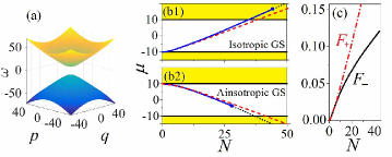
Figure 1: (a) The bandgap structure, as per Eq. (6) with $(\lambda,\Omega)=(1,10)$. The same values of $\Omega$ and $\lambda$ are used below throughout the paper. (b) The chemical potential of the isotropic (b1) and anisotropic (b2) 2D solitons, vs. their total norm, $N$, defined as per Eq. (9). Yellow areas are spectral bands, with the white gap between them. Blue solid and black dotted curves are, respectively, numerically found stable branches and their unstable extensions. The stable branch of isotropic solitons [semi-vortices, see Eq. (10)] traverses the bandgap and extends, in the form of ESs, to the upper band. It is stable at $N<N_{\max}\approx 45.0$. The branch of anisotropic solitons extends into the lower band, but its stable segment terminates in the gap, at $N=N_{\max}\approx 28.2$. Red dashed curves are semi-analytical predictions based on Eq. (16). (c) The share of the total norm in the vortex component, $F_{\mp}=N_{\mp}/N$, vs. $N$ for the isotropic ($-$) and anisotropic ($+$) solitons. Note that figure and all others refer to the scaled norm, while the actual number of atoms in the respective BECis $N_{\mathrm{at}}\sim 10^{3}N$, see Eq. (18). In all the panels, we have fixed $\kappa=0.1$.

Furthermore, Eqs. (7) and (8) with the isotropic DDI kernel given by Eq. (2) admit solutions with an exact structure of semi-vortices Sakaguchi ; HP ; Sherman , i.e., isotropic complexes with zero vorticity $S=0$ in component $u_{+}$, and vorticity $S=1$ in $u$:

$$u_{+}=U_{+}(r),~{}u_{-}=U_{-}(r)e^{i\theta},$$ (10)

where $\left(r,\theta\right)$ are the polar coordinates in the $\left(x,y\right)$ plane, and radial functions $U_{\pm}(r)$ are real. Indeed, the substitution of the semi-vortex ansatz (10) in Eqs. (7) and (8) yields, after performing the angular integration in the DDI terms, to the following equations which include solely the radial coordinate:

$$\mu U_{+}=\lambda\left(\frac{dU_{-}}{dr}+\frac{1}{r}U_{-}\right)-\Omega U_{+}+\left(gU_{+}^{2}+\tilde{g}U_{-}^{2}\right)U_{+}$$

$$+\kappa U_{+}\int_{0}^{\infty}\varrho(r,r^{\prime})\left[U_{+}^{2}(r\mathbf{{}^{\prime}})+U_{-}^{2}(r\mathbf{{}^{\prime}})\right]r^{\prime}dr\mathbf{{}^{\prime}}.$$ (11)

$$\mu U_{-}=-\lambda\frac{dU_{+}}{dr}+\Omega U_{-}+\left(gU_{-}^{2}+\tilde{g}U_{+}^{2}\right)U_{-}$$

$$+\kappa U_{-}\int\varrho(r,r^{\prime})\left[U_{+}^{2}(r\mathbf{{}^{\prime}})+U^{2}_{-}(r\mathbf{{}^{\prime}})\right]r^{\prime}dr\mathbf{{}^{\prime}},$$ (12)

where the effective radial kernel is

$$\varrho(r,r^{\prime}) = \frac{2E(k)}{\sqrt{\epsilon^{2}+\left(r+r^{\prime}\right)^{2}}\left[\epsilon^{2}+\left(r-r^{\prime}\right)^{2}\right]}.$$

$$k \equiv \frac{2\sqrt{rr^{\prime}}}{\sqrt{\epsilon^{2}+\left(r+r^{\prime}\right)^{2}}}.$$ (13)

Here, $E(k)$ is the standard complete elliptic integral of the second kind with modulus $k$.

Numerical results presented in the next section, see Figs. 2(a,b,c) and 3(a1,a2,a3), confirm that Eqs. (7) and (8) with the isotropic kernel indeed give rise to the two-component solitons whose structure precisely conforms to ansatz (10). Furthermore, it is demonstrated below that the anisotropic kernel gives rise, as a matter of fact, to deformed patterns of the same semi-vortex type, with $S=0$ in component $u_{-}$ and $S=-1$ in $u_{+}$, see Figs. 2(d,e,f) and 3(b1,b2,b3) below.

III Families of gap solitons and embedded solitons

III.1 Isotropic and anisotropic solitons near edges of the bandgap

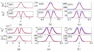
Figure 2: Comparison between cross sections, drawn along $x=0$, of stable isotropic solitons [semi-vortices, see Eq. (10)] (a,b,c) and anisotropic (d,e,f) solitons, as found in the numerical form (blue solid curves), and predicted by Eqs. (15) and (16) (red dash curves). (a) A GS with $N=2.013$ and $\mu=-9.7$. (b) A GS with $N=21.37$ and $\mu=1.72$. (c) An ES with $N=44.47$, $\mu=16.65$, located close to the stability boundary (the blue dot) of isotropic solitons. (d) A GS with $N=2.0043$, $\mu=9.935$. (e) A GS with $N=16.12$, $\mu=4.06$. (f) A GS with $N=28.17$, $\mu=-3.78$, located close to the stability boundary of anisotropic solitons.

Close to edges of the bandgap of dispersion relation (6), i.e., at

$$\mu=\mp\left(\Omega-\delta\mu\right),0<\delta\mu\ll\Omega~{},$$ (14)

the two-component problem can be reduced to one of those previously solved for the single component in the semi-infinite gap Pedri ; Tikhonenkov . Close to the bottom (top) edge, Eq. (8) for $u_{-}$ ($u_{+}$) makes it possible to eliminate this component in favor of $u_{+}$ ($u_{-}$):

$$u_{\mp}\approx\left(\lambda/2\Omega\right)\left({\partial}_{x}\pm i\partial_{y}\right)u_{\pm}.$$ (15)

In particular, for the isotropic semi-vortex represented by ansatz (10), Eq. (15) amounts to $U_{-}(r)\approx\left(\lambda/2\Omega\right)dU_{+}/dr$.

Substituting relation (15) in Eq. (8) for $u_{\pm}$, one arrives at an equation for the single component:

$$\delta\mu\cdot u_{\pm}={\frac{\lambda^{2}}{2\Omega}}\nabla^{2}u_{\pm}\pm g|u_{\pm}|^{2}u_{\pm}\pm\kappa u_{\pm}(\mathbf{r})\int R(\mathbf{r}-\mathbf{r^{\prime}})|u_{\pm}(\mathbf{r^{\prime}})|^{2}d\mathbf{r^{\prime}},$$ (16)

where $\nabla^{2}=(\partial_{x}+i\partial_{y})(\partial_{x}-i\partial_{y})\equiv\partial_{x}^{2}+\partial_{y}^{2}$ appears as a square of the SOC operator from Eqs. (4) and (5). It is easy to see that the same $\nabla^{2}$ is produced by squaring the SOC operator which presents a general combination of the Rashba and Dresselhaus terms.

Along with Eq. (16), it is relevant to consider its time-dependent version,

$$\mp i\frac{\partial}{\partial t}\tilde{u}_{\pm}={\frac{\lambda^{2}}{2\Omega}}\nabla_{\pm}^{2}\tilde{u}\pm g|\tilde{u}_{\pm}|_{\pm}^{2}\tilde{u}\pm\kappa\tilde{u}_{\pm}(\mathbf{r})\int R(\mathbf{r}-\mathbf{r^{\prime}})|\tilde{u}_{\pm}(\mathbf{r^{\prime}})|^{2}d\mathbf{r^{\prime}},$$ (17)

where $\tilde{u}_{\pm}\left(x,y,t\right)\equiv\exp\left(\pm i\Omega t\right)~{}u\left(x,y,t\right)$. In particular, Eq. (17) is used below to test stability of various solitons generated by Eq. (16).

If the contact nonlinear term $\sim g$ is present in Eq. (16), while the DDI is absent ($\kappa=0$), this equation produces no solitons in the case of the effective self-defocusing, $\pm g<0$ (recall we define $\Omega$ to be positive). In the case of the local self-focusing,

$\pm g>0$, Eq. (16) produces unstable Townes solitons Townes . This argument suggests that the contact interaction of either sign, in the absence of the DDI, cannot support stable solitons in the present system. As mentioned above, this expectation is fully corroborated by numerical results (not shown here in detail).

Proceeding to the opposite case, when the DDI is present, while the contact interaction is absent ($g=0$), we note that, near the bottom edge of the bandgap, Eq. (16) for $u_{+}$, with $\kappa>0$ and the isotropic kernel, $R=R_{\mathrm{iso}}(\mathbf{r}-\mathbf{r^{\prime}})$, gives rise to the ground state in the form an axisymmetric bright soliton with zero vorticity Pedri , while the respective smaller component $u_{-}$, produced by Eq. (15), features vortical structure $\sim re^{i\theta}$ (at small $r$), conforming to the semi-vortex structure of the isotropic GS, as given by Eq. (10). In fact, in this case, the 2D integration in Eq. (16) can be reduced to the radial-only integration, with kernel $R_{\mathrm{iso}}(\mathbf{r}-\mathbf{r^{\prime}})$ substituted by the effective radial one, as done above, in the general form, in Eq. (13).

On the other hand, near the top edge of the bandgap, Eq. (16) for $u_{-}$, with $\kappa>0$ and the anisotropic kernel taken as per Eq. (3), gives rise to the ground state in the form of the 2D anisotropic bright soliton, as previously demonstrated in Ref. Tikhonenkov , while Eq. (15) produces a smaller component, $u_{+}$, in the form of an anisotropic vortex. Overall, the anisotropic GS constructed in this form seems as a deformed semi-vortex, as corroborated by numerically exact results displayed below in Fig. 3(b1,b2,b3).

III.2 Numerical findings for generic two-component solitons

The above results predict that the isotropic DDI for dipoles polarized perpendicular to the $\left(x,y\right)$ plane, and the anisotropic DDI for the in-plane polarization, support, severally, stable isotropic GSs [with the semi-vortex structure, as per Eq. (10)] and anisotropic 2D GSs, with $\mu$ taken, respectively, close to the bottom or top edge of the bandgap. These predictions have been corroborated by numerical solutions of Eqs. (7) and (8). The numerical results are collected in Fig. 1(b1,b2) for the system which does not include the contact interaction [$g,\tilde{g}=0$ in Eqs. (7) and (8)]. The results clearly demonstrate that the quasi-analytical approximations remain valid not only close to the edges, but actually across the entire bandgap, and extend, as ESs (see further details below), into the bands.

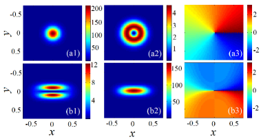
Figure 3: (a1,a2) Density patterns of $u_{+}$ and $u_{-}$ (zero-vorticity and vortex components, respectively) for a stable isotropic GS (semi-vortex) with $N=21.37$, $\mu=1.17$. (a3) The phase structure of $u_{-}$. (b1-b3) The same for a stable anisotropic GS (deformed semi-vortex) with $N=22.02$, $\mu=0.016$).

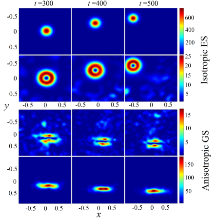
Figure 4: Evolution of an unstable isotropic ES, with $N=56.43$, $\mu=24.84$ (a), and of an anisotropic GS with $N=34.5$, $\mu=-8$ (b). Density snapshots of the zero-vorticity and vortex components are shown in the top and bottom panels, respectively, for the isotropic soliton, and vice versa for the anisotropic one.

Numerical solutions of Eq. (8) were produced by means of the squared-operator method Jianke2007 . The scaling invariances of Eqs. (4) and (8) were used to fix $\Omega=10$, $\lambda=1$, and $\kappa=0.1$. Generic results were produced fixing the regularization parameter as $\epsilon=0.5$ (with other reasonable values of $\epsilon$, similar results have been obtained), while the total norm, $N$, was varied as an essential control parameter. The stability of the GS families was identified by means of systematic simulations of the perturbed evolution (the distinction between stable and unstable states could be easily detected, as numerical truncation errors were sufficient to trigger the growth of the instability, if any). As concerns the asymptotic equation (16), its solutions of were produced by applying the imaginary-time method ITM to its time-dependent version given by Eq. (17). Comparison of shapes of stable solitons, as found from Eqs. (7) and (8), and, on the other hand, from the simplified equations (16) and (17), is displayed in Fig. 2.

Branches of isotropic and anisotropic solitons are characterized by $\mu(N)$ dependences displayed in Fig. 1(b1,b2), along with the semi-analytical counterparts of these dependences. It has been thus found that the stable branch of the isotropic GSs extends, across the full bandgap, into the upper Bloch band abutting on the bandgap, as a family of ESs, which may exist, under certain conditions, in spectral bands Jianke1999 . In particular, a model supporting ESs in a 2D system was reported in Ref. 2D-ES . With the increase of $N$, the isotropic-ES branch loses its stability inside of the Bloch band, at $N_{\max}\approx 45$ ($\mu\approx 16.7$). At $N>N_{\max}$, the branch extends indefinitely into the band in an unstable form. On the contrary, the stability of the anisotropic GSs terminates still in the bandgap, at $N_{\max}\approx 28.2$ ($\mu\approx$ $-3.8$), the ES continuation of this branch being fully unstable. The robustness of the solitons in the present system is further attested to by the fact that unstable ones, both isotropic and anisotropic, do not suffer destruction, their vortex component keeping its vorticity: as shown in Fig. 4, unstable solitons commence spontaneous motion, instead of destruction, emitting small amounts of radiation from the vortex component. The evolution of the weakly unstable isotropic ESs (recall all the isotropic GS are stable) does not break their circular symmetry either.

As said above, isotropic GSs are built as semi-vortices [defined as per Eq. (10)], i.e., bound states of zero-vorticity and vortex components, as can be clearly seen in Figs. 3(a1-a3). The extension of the GS solutions in the ES form keeps the semi-vortex shape as well. Although no exact ansatz for a vortex structure is available for anisotropic GSs, Figs. 3(b1-b3) clearly demonstrate that the anisotropic GSs (and their ES extension) feature the shape of deformed semi-vortices. An essential peculiarity of the semi-vortices is that their vortex component carries a relatively small share of the total norm, in comparison with the zero-vorticity counterpart, as shown in Fig. 1(c) for the isotropic and anisotropic semi-vortices alike.

The stable isotropic solitons shown above, with vorticities $(S_{+},S_{-})=(0,1)$ in their large and small components, are fundamental states, as the system cannot produce any state with a simpler structure. However, it is possible to look for more complex modes (excited states). To generate them near the bottom edge of the bandgap, one can use, as a seed, isotropic vortex-solitons solutions of Eq. (16) for the large component, $u_{+}$, with vorticities $S_{+}=\pm 1$, which are known from the study of the single-component dipolar BEC Tikhon2 . Then, Eq. (15) generates vorticity $S_{-}=S_{+}+1$ in the small $u_{-}$ component. We have found that both species of the resulting composite modes, with $(S_{+},S_{-})=(1,2)$ and $(-1,0)$, are unstable against splitting into a pair of fragments (not shown here in detail). In fact, splitting is a common instability mode of vortex solitons old-review ; Dumitru ; recent-review ; Skryabin , although nonlocality may stabilize some of them Kiev ; Tikhon2 .

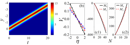
Figure 5: (a) Stable motion of an isotropic GS (semi-vortex) with $N=5.1$ and $\mu=-8.41$, which was kicked in the $y$-direction with strength $\eta=+3$, as per initial conditions (20). (b) Velocity $V_{x}$ of the isotropic GS, kicked along $x$, versus $\eta$, for $N=2.01$ (black squares), $21.36$ (red circles) and $44.47$ (blue triangles), respectively. (c1,c2) Negative and positive effective masses, $M_{x}$ and $M_{y}$, for isotropic and anisotropic solitons, respectively.

III.3 Physical parameters for the gap solitons in the Bose-Einstein condensate

It is relevant to estimate actual parameters of the BEC solitons which can be created according to the results reported above in the scaled form. To this end, we translate the results into physical units corresponding to the experimental realization of SOC Zeeman ; Cr ; Xunda ; Drummond-Pu , taking values of the magnetic moment for ⁵²Cr or ¹⁶⁴Dy atoms, and the strength of the transverse trapping potential $\omega_{\perp}\sim 100$ Hz. We thus conclude that the stable quasi-2D solitons may be created with the number of atoms in the range from $N_{\mathrm{at}}\sim 10^{3}$ (near edges of the bandgap)   to $N_{\mathrm{at}}\sim 10^{4}$ (deeper in the bandgap), and physical lateral sizes $l_{\mathrm{phys}}\sim 10$ $\mathrm{\mu}$m. The corresponding relations between the physical quantities and scaled ones displayed in Figs. 1-7 is

$$N_{\mathrm{at}}\sim 10^{3}N,~{}\left(x,y\right)_{\mathrm{phys}}\sim(x,y)\times 20\mathrm{\mu m~{}.}$$ (18)

Further, the magnetic field necessary for inducing the appropriate ZS is estimated as $H\sim 0.1-1$ G. In addition to the magnetic realization, the use of a spinor BEC built of small molecules carrying electric dipole moments electric may be feasible too. Another possibility for the realization of the stable 2D solitons predicted above is to use the DDI between moments induced by an external dc magnetic or electric field induced .

IV Mobility and collisions of the isotropic and anisotropic solitons

Soliton mobility in the system under the consideration is a nontrivial issue, as Eqs. (4) and (5) are not Galilean invariant, although they conserve the total momentum,

$$\mathbf{P}=i\int\left[\left(\nabla\phi_{+}^{\ast}\right)\phi_{+}+\left(\nabla\phi_{-}^{\ast}\right)\phi_{-}\right]d\mathbf{r},$$ (19)

and their asymptotic version, which amounts to the single equation (17), remains Galilean invariant. The mobility was tested, in the framework of the system without the contact interactions ($g=\tilde{g}=0$), by applying kick $\eta$ to stable quiescent solitons in the $x$ or $y$ direction, which correspond to simulating Eqs. (4) and (5) with input

$$\phi_{\pm}(x,y,t=0)=u_{\pm}(x,y)\left\{e^{i\eta x},e^{i\eta y}\right\},$$ (20)

the components of the respective momentum (19) being $P_{x,y}=N\eta$. An example of stable motion of a kicked isotropic GS (semi-vortex) is shown in Fig. 5(a). The velocity of the moving isotropic soliton, $V_{x}$, is displayed in Fig. 5(b) as a function of the kick’s magnitude, $\eta$. It is seen that the mass of kicked isotropic GSs is negative, as they move in the direction opposite to the kick. It is relevant to mention that the negative dynamical mass is a generic feature of GSs known in other settings, including 2D GSs HS ; plasmon .

The effective mass of the isotropic solitons in the $x$ and $y$ directions, defined as $M_{x,y}(N)=P_{x.y}/V_{x,y}$, is displayed in Fig. 5(c1) as a function of $N$ (strictly speaking, the motion makes the soliton slightly anisotropic). Naturally, the mass increases almost linearly with the norm. Close to the bottom edge of the bandgap, where $N$ is very small, the mass is isotropic, $M_{x}\approx M_{y}$, as the corresponding equation (16) is isotropic too. Farther from the bandgap edge, the mass features a weak anisotropy. On the other hand, the anisotropic solitons feature a positive mass, which also grows almost linearly with $N$, as shown in Fig. 5(c2). In the course of its motion, the kicked solitons show very weak transverse displacement, due to the “Magnus force” acting on the small vortical component Magnus . Additional high-accuracy simulations are needed to study the latter effect in detail.

It is natural too to study collisions between stable GSs set in motion by opposite kicks $\pm\eta$. The simulations reveal three generic outcomes of the collisions, for the isotropic and anisotropic solitons alike: merger into a single breather [Figs. 6(a1,a2)], elastic collision [Figs. 6(c1,c2)], and transformation into diffracting quasi-linear beams [Figs. 6(b1,b2)], at, small, large, and intermediate values of $\eta$, respectively.

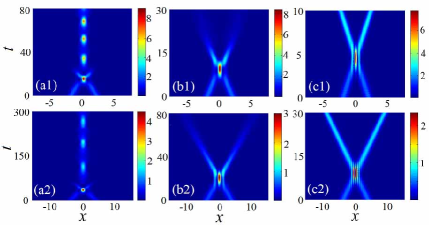
Figure 6: (a1-c1): Collisions between stable isotropic GSs with $N=2.013,\mu=-9.7$. The solitons were set in motion by opposite kicks: $\eta=\pm 1$ (a1), $\pm 2$ (b1), $\pm 5$ (c1). (a2-c2): The same for anisotropic GSs, with $N=2.004,\mu=9.94$, and kicks $\eta=\pm 1$ (a2), $\pm 2$ (b2), $\pm 5$ (c2).

V Effects of the contact interaction

The local mean-field nonlinearity, induced by interatomic collisions, is always present in the bosonic gas, therefore it is relevant to explore effects of the contact interaction on the soliton families obtained above in the absence of the contact terms in Eqs. (7) and (8). Here, we perform this analysis in the framework of the asymptotic equations (16) and (17), as they are sufficient to capture main effects produced by the local nonlinearity, as shown below.

First, Eq. (16), that includes the contact-interaction term $\sim g$, implies that, due to the possibility of the critical collapse Townes in the same 2D equation, the norm of wave function $u_{\pm}$ cannot exceed a critical value, which is determined by the scaled norm of the Townes’ soliton, $N_{\mathrm{Townes}}\approx 5.85$ Townes , viz., ${N_{\pm}<N_{\mathrm{Townes}}/}\left(\pm g\Omega\right)$. In other words, for given norm $N$, isotropic and anisotropic self-trapped modes exist, respectively, at

$${g<g_{\mathrm{Townes}}^{\mathrm{(iso)}}={N_{\mathrm{Townes}}}/}\left({\Omega N}\right),~{}{g>g_{\mathrm{Townes}}^{\mathrm{(aniso)}}=-{N_{\mathrm{Townes}}}/}\left({\Omega N}\right)$$ (21)

(recall $\Omega=10$ is fixed in this paper).

Furthermore, inside the existence regions (21), systematic simulations of Eq. (17) have revealed an intrinsic stability boundary, $g=$ $g_{\mathrm{cr}}^{(\pm)}\approx\pm 0.25$, such that the isotropic and anisotropic stationary GSs are stable, respectively, at $g<$ $g_{\mathrm{cr}}^{(+)}$ and $g>g_{\mathrm{cr}}^{(-)}$, while in the remaining intervals, $g_{\mathrm{cr}}^{(+)}<g<$${g_{\mathrm{Townes}}^{\mathrm{(iso)}}}$ and ${g_{\mathrm{Townes}}^{\mathrm{(aniso)}}<g<}$$g_{\mathrm{cr}}^{(-)}$, the GSs are unstable, spontaneously transforming into persistent breathers, as shown in Fig. 7. Thus, we conclude that the stationary GSs exist and remain completely stable when the arbitrarily strong contact interaction is self-repulsive, in terms of Eqs. (16) and (17) (which corresponds to $g<0$ and $g>0$ for the isotropic and anisotropic GSs, respectively), being compensated by the effectively attractive DDI. In the limit of very strong local self-attraction, the solitons become very broad, corresponding to $\delta\mu\rightarrow 0$ in terms of Eq. (16), i.e., $\mu\rightarrow-\Omega$ and $\mu\rightarrow+\Omega$, in terms of Figs. 7(c) and (d), respectively. Note an essential difference of these limits from those shown in Figs. 1(b1) and (b2): in the latter case, the soliton’s norm vanishes at the edges of the bandgap, while in the cases displayed in Figs. 7(c) and (d) the soliton branches keep the fixed finite norm, $N_{\pm}=2$.

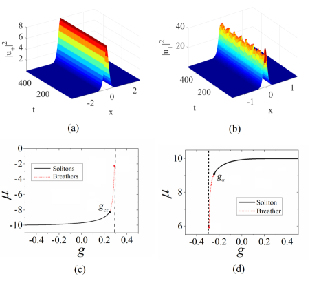
Figure 7: (a,b) Simulations of the evolution of isotropic GSs, in the framework of Eqs. (4) and (5) which include the local nonlinear terms with $g=0.2$ (a) and $g=0.28$ (b), while the norm of the large zero-vorticity component is fixed as $N_{+}=2$. The results are displayed for the cross section of $\left|\phi_{+}(x,y,t)\right|^{2}$ at $y=0$. (c) The chemical potential of isotropic solitons with $N_{+}=2$ versus $g$. Black solid and red dotted segments represent, severally, stable stationary solitons and persistent breathers, which replace unstable solitons at $g>g_{\mathrm{cr}}\approx 0.25$. The vertical dashed line is the existence boundary for self-trapped modes, where the collapse sets in, $g=g_{\mathrm{Townes}}^{\mathrm{(iso)}}\approx 0.29$, see Eq. (21). (d) The chemical potential of the anisotropic solitons with $N_{-}=2$ versus $g$. The meaning of the black solid and red dotted segments is the same as as in (c), the boundary between them being $g_{\mathrm{cr}}\approx-0.25$, while the existence/collapse boundary is marked by the vertical dashed line at $g=g_{\mathrm{Townes}}^{\mathrm{(aniso)}}\approx-0.29$.

To explicitly compare strengths of the competing contact interactions and DDI, we define the relative strength,

$$\epsilon_{\mathrm{dd}}\equiv g_{\mathrm{eff}}^{(\mathrm{iso,aniso})}/g,$$ (22)

where $g_{\mathrm{dd}}^{(\mathrm{iso,aniso})}$ are effective DDI coefficients for the isotropic and the anisotropic GSs, respectively, which are defined, for the definiteness’ sake, at centers of the solitons, as follows:

$$\kappa u_{+}(\mathbf{r}=0)\int R_{\mathrm{iso}}(0-\mathbf{r^{\prime}})|u_{+}(\mathbf{r^{\prime}})|^{2}d\mathbf{r^{\prime}\equiv}g_{\mathrm{eff}}^{(\mathrm{iso})}|u_{+}(\mathbf{r}=0)|^{2}u_{+}(\mathrm{r}=0),$$ (23)

$$\kappa u_{-}(\mathbf{r}=0)\int R_{\mathrm{aniso}}(0-\mathbf{r^{\prime}})|u_{-}(\mathbf{r^{\prime}})|^{2}d\mathbf{r^{\prime}\equiv}g_{\mathrm{eff}}^{(\mathrm{aniso})}|u_{-}(\mathbf{r}=0)|^{2}u_{-}(\mathrm{r}=0).$$ (24)

Here, we adopt conditions $|u_{+}(\mathbf{r})|^{2}\gg|u_{-}(\mathbf{r})|^{2}$ and $|u_{-}(\mathbf{r})|^{2}\gg|u_{+}(\mathbf{r})|^{2}$ for the isotropic and anisotropic GSs, respectively, as Figs. 7(c) and (d) clearly demonstrates that these conditions hold at the critical (most essential) points.

The so defined relative DDI strengths (22) are displayed, as functions of $g$, in Fig. 8, for isotropic and anisotropic GSs at $g>0$ and $g<0$, respectively. A natural conclusion is that the GSs suffer the destabilization when the DDI becomes too weak in comparison with the contact interaction.

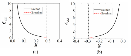
Figure 8: The relative strengths of the DDI, $\epsilon_{\mathrm{dd}}$, defined as per Eqs. (22)-(24), are displayed as functions of $g$. Black solid and red dotted segments, as well as the vertical dashed lines, have the same meaning as in Fig. 7. (a) The $\epsilon_{\mathrm{dd}}(g)$ dependence for isotropic solitons with $N_{+}=2$. (b) The same for anisotropic solitons with $N_{-}=2$.

On the contrary to the setting with the competing contact interaction and DDI, the interplay of the local and nonlocal nonlinear interactions with identical signs leads to the destabilization of the solitons in the present system, as is shown by Figs. 7(c,d). Overall, the present situation qualitatively resembles that reported in Ref. Minhang , in which a binary BEC represented a mixture of two atomic states coupled by a microwave field. In such a setting, nonlocal attraction between the components, mediated by the microwave field, was sufficient for the existence and stability of two-component solitons in the presence of arbitrarily strong local self- and cross- repulsion.

VI Conclusion

The objective of this work is to propose a setting for the creation of stable quasi-2D GSs (gap solitons) and ESs (embedded solitons) in free space. The system is based on the spinor dipolar BEC, whose components are coupled by the SOC (spin-orbit interaction). For quasi-2D states, the kinetic-energy terms in the spinor GPEs are negligible in comparison with SOC, which gives rise to simplified couple-mode equations, with the bandgap provided by the ZS (Zeeman splitting). Stable isotropic and anisotropic 2D solitons were thus found, in the quasi-analytical and numerical forms, for the dipoles polarized perpendicular and parallel to the system’s plane, respectively. Both families continue as ESs into adjacent spectral bands, the isotropic-ES branch being partly stable. Mobility and collisions of the solitons were studied too, concluding that the mass of the isotropic/anisotropic ones is negative/positive. Effects of contact interactions, added to the DDI (dipole-dipole interaction), were studied too, with a conclusion that the stationary GSs persist and remain stable in the presence of the arbitrarily strong local self- and cross-component repulsion, compensated by the effectively attractive DDI.

A challenging possibility is to extend the present analysis from solitons to “quantum droplets” in binary dipolar BEC, in the presence of SOC. “Droplets” stabilized by beyond-the-mean-field effects were recently created in single-component dipolar condensates droplets .

- (1) B. J. Eggleton, R. E. Slusher, C. M. de Sterke, P. A. Krug, and J. E. Sipe, Bragg Grating solitons, Phys. Rev. Lett. 76, 1627-1630 (1996).
- (2) D. Mandelik, R. Morandotti, J. S. Aitchison, and Y. Silberberg, Gap solitons in waveguide arrays, Phys. Rev. Lett. 92, 093904 (2004).
- (3) J. W. Fleischer, M. Segev, N. K. Efremidis, and D. N. Christodoulides, Observation of two-dimensional discrete solitons in optically induced nonlinear photonic lattices, Nature (London) 422, 147-150 (2003).
- (4) C. M. de Sterke and J. E. Sipe, Gap solitons, Progr. Optics 33, 203-260 (1994).
- (5) I. L. Garanovich, S. Longhi, A. A. Sukhorukov, Y. S. Kivshar, Light propagation and localization in modulated photonic lattices and waveguides, Phys. Rep. 518, 1 (2012)
- (6) F. Lederer, G. I. Stegeman, D. N. Christodoulides, G. Assanto, M. Segev, and Y. Silberberg, Discrete solitons in optics,Phys. Rep. 463, 1 (2008).
- (7) V. A. Brazhnyi and V. V. Konotop, Theory of nonlinear matter waves in optical lattices, Mod. Phys. Lett. B 18, 627 (2994); O. Morsch and M. Oberthaler, Dynamics of Bose-Einstein condensates in optical lattices, Rev. Mod. Phys. 78, 179 (2006).
- (8) B. Eiermann, Th. Anker, M. Albiez, M. Taglieber, P. Treutlein, K.-P. Marzlin, and M. K. Oberthaler, Bright Bose-Einstein Gap Solitons of Atoms with Repulsive Interaction, Phys. Rev. Lett. 92, 230401 (2004).
- (9) E. A. Ostrovskaya, J. Abdullaev, M. D. Fraser, A. S. Desyatnikov, and Yu. S. Kivshar, Self-localization of polariton condensates in periodic potentials, Phys. Rev. Lett. 110, 170407 (2013); E. A. Cerda-Méndez, D. Sarkar, D. N. Krizhanovskii, S. S. Gavrilov, K. Biermann, M. S. Skolnick, and P. V. Santos, Exciton-polariton gap solitons in two-dimensional lattices, ibid. 111, 146401 (2013).
- (10) B. A. Malomed, D. Mihalache, F. Wise, and L. Torner, Spatiotemporal optical solitons. J. Optics B: Quant. Semicl. Opt. 7, R53-R72 (2005); Viewpoint: On multidimensional solitons and their legacy in contemporary Atomic, Molecular and Optical physics, J. Phys. B: At. Mol. Opt. Phys. 49, 170502 (2016).
- (11) D. Mihalache, Linear and nonlinear light bullets: Recent theoretical and experimental studies, Rom. J. Phys. 57, 352 (2012)
- (12) B. A. Malomed, Multidimensional solitons: Well-established results and novel findings, Eur. Phys. J. Special Topics, 225, 2507-2532 (2016).
- (13) Y.-J. Lin, K. Jiménez-García, I. B. Spielman, Spin-orbit-coupled Bose-Einstein condensates, Nature (London), 471, 83 (2011);Y. Zhang, L. Mao, and C. Zhang, Mean-Field Dynamics of Spin-Orbit Coupled Bose-Einstein Condensates,Phys. Rev. Lett. 108, 035302 (2012).
- (14) Y. V. Kartashov, B. A. Malomed, V. V. Konotop, V. E. Lobanov, and L. Torner, Stabilization of solitons in bulk Kerr media by dispersive coupling, Opt. Lett. 40, 1045-1048 (2015).
- (15) H. Sakaguchi and B. A. Malomed, One- and two-dimensional solitons in -symmetric systems emulating the spin-orbit coupling, New J. Phys. 18, 105005 (2016).
- (16) Y. V. Kartashov, V. V. Konotop, and F. Kh. Abdullaev, Gap Solitons in a Spin-Orbit-Coupled Bose-Einstein Condensate, Phys. Rev. Lett. 111, 060402 (2013); Y. V. Kartashov and V. V. Konotop, Solitons in Bose-Einstein condensates with helicoidal spin-orbit coupling, ibid. 118, 190401 (2017). X. Zhu, H. Li, Z. Shi, Defect matter-wave gap solitons in spin Corbit-coupled Bose CEinstein condensates in Zeeman lattices, Phys. Lett. A 380, 3253 (2017).
- (17) V. E. Lobanov, Y. V. Kartashov, and V. V. Konotop, Fundamental, multipole, and half-vortex gap solitons in spin-orbit coupled Bose-Einstein condensates, Phys. Rev. Lett. 112, 180403 (2014).
- (18) H. Sakaguchi, B. Li, and B. A. Malomed, Creation of two-dimensional composite solitons in spin-orbit-coupled self-attractive Bose-Einstein condensates in free space, Phys. Rev. E 89, 032920 (2014).
- (19) Y.-C. Zhang, Z.-W. Zhou, B. A. Malomed, and H. Pu, Stable solitons in three-dimensional free space without the ground state: Self-trapped Bose-Einstein condensates with spin-orbit coupling, Phys. Rev. Lett. 115, 253902 (2015).
- (20) D. L. Campbell, G. Juzeliūnas, and I. B. Spielman, Realistic Rashba and Dresselhaus spin-orbit coupling for neutral atoms, Phys. Rev. A 84, 025602 (2011).
- (21) T.-L. Ho, Spinor Bose condensates in optical traps, Phys. Rev. Lett. 81, 742-745 (1998).
- (22) Y. Deng, J. Cheng, H. Jing, C.-P. Sun, and S. Yi, Spin-orbit-coupled dipolar Bose-Einstein condensates, Phys. Rev. Lett. 108, 125301 (2012).
- (23) R. M. Wilson, B. M. Anderson, and C. W. Clark, Meron ground state of Rashba Spin-Orbit-Coupled dipolar bosons, Phys. Rev. Lett. 111, 185303 (2013); S. C. Ji, L. Zhang, X. T. Xu, Z. Wu, Y. J. Deng, S. Chen, and J. W. Pan, Softening of roton and phonon modes in a Bose-Einstein condensate with spin-orbit coupling, ibid. 114, 105301 (2015); Y. Xu, Y. Zhang, and C. Zhang, Bright solitons in a 2D spin-orbit-coupled dipolar Bose-Einstein condensate, Phys. Rev. A 92, 013633 (2015); X. Jiang, Z. Fan, Z. Chen, W. Pang, Y. Li, and B. A. Malomed, Two-dimensional solitons in dipolar Bose-Einstein condensates with spin-orbit coupling, ibid. 93, 023633 (2016); T. Oshima and Y. Kawaguchi, Spin Hall effect in a spinor dipolar Bose-Einstein condensate, ibid. 93, 053605 (2016).
- (24) H. Sakaguchi, E. Ya. Sherman, and B. A. Malomed, Vortex solitons in two-dimensional spin-orbit coupled Bose-Einstein condensates: Effects of the Rashba-Dresselhaus coupling and the Zeeman splitting, Phys. Rev. E 94, 032202 (2016).
- (25) J. Yang, B. A. Malomed, and D. J. Kaup, Embedded solitons in second-harmonic-generating systems, Phys. Rev. Lett. 83, 1958 (1999); A. R. Champneys, B. A. Malomed, J. Yang, and D. J. Kaup, “Embedded solitons” : solitary waves in resonance with the linear spectrum, Physica D 152-153, 340-354 (2001).
- (26) D. Cai, A. R. Bishop, and N. Grønbech-Jensen, Localized states in discrete nonlinear Schrödinger equations, Phys. Rev. Lett. 72, 591-595 (1994); H. Sakaguchi and B. A. Malomed, Dynamics of positive- and negative-mass solitons in optical lattices and inverted traps, J. Phys. B: At. Mol. Opt. Phys. 37, 1443-1459 (2004); M. Salerno, V. V. Konotop, and Yu. V. Bludov, Long-living Bloch oscillations of matter waves in periodic potentials, Phys. Rev. Lett. 101, 030405 (2008); E. A. Cerda-Méndez, D. Sarkar, D. N. Krizhanovskii, S. S. Gavrilov, K. Biermann, M. S. Skolnick, and P. V. Santos, Exciton-polariton gap solitons in two-dimensional lattices, ibid. 111, 146401 (2013).
- (27) Y. A. Bychkov and E. I. Rashba, Oscillatory effects and the magnetic susceptibility of carriers in inversion layers, J. Phys. C 17, 6039 (1984).
- (28) Y. Xu, Y. Zhang, and B. Wu, Bright solitons in spin-orbit-coupled Bose-Einstein condensates, Phys. Rev. A 87, 013614 (2013).
- (29) V. Achilleos, D. J. Frantzeskakis, P. G. Kevrekidis, and D. E. Pelinovsky, Matter-Wave Bright Solitons in Spin-Orbit Coupled Bose-Einstein Condensates, Phys. Rev. Lett. 110, 264101 (2013).
- (30) G. Chen, Y. Liu, H. Wang, Mixed-mode solitons in quadrupolar BECs with spin Corbit coupling, Commun. Nonlinear Sci. Numer. Simulat. 48, 318 (2017).
- (31) S. Giovanazzi, A. Görlitz, and T. Pfau, Tuning the dipolar interaction in quantum gases, Phys. Rev. Lett. 89, 130401 (2002).
- (32) S. Sinha and L. Santos, Cold dipolar gases in quasi-one-dimensional geometries, Phys. Rev. Lett. 99, 140406 (2007).
- (33) J. Cuevas, B. A. Malomed, P. G. Kevrekidis, and D. J. Frantzeskakis, Solitons in quasi-one-dimensional Bose-Einstein condensates with competing dipolar and local interactions, Phys. Rev. A 79, 053608 (2009).
- (34) J. Huang, X. Jiang, H. Chen, Z. Fan, W. Pang, and Y. Li, Quadrupolar matter-wave soliton in two-dimensional free space, Front. Phys. 10, 100507 (2015).
- (35) B. Ramachandhran, B. Opanchuk, X.-J. Liu, H. Pu, P. D. Drummond, and H. Hu, Half-quantum vortex state in a spin-orbit-coupled Bose-Einstein condensate, Phys. Rev. A 85, 023606 (2012).
- (36) I. Tikhonenkov, B. A. Malomed, and A. Vardi, Anisotropic Solitons in Dipolar Bose-Einstein Condensates, Phys. Rev. Lett. 100, 090406 (2008); P. Köberle, D. Zajec, G. Wunner, and B. A. Malomed, Creating two-dimensional bright solitons in dipolar Bose-Einstein condensates, Phys. Rev. A 85, 023630 (2012).
- (37) J. Yang and T. I. Lakoba, Universally-convergent squared-operator iteration methods for solitary waves in general nonlinear wave equations, Stud. Appl. Math. 118, 153 (2007).
- (38) H.-Y. Hui, Y. Zhang, C. Zhang, and V. W. Scarola, Superfluidity in the absence of kinetics in spin-orbit-coupled optical lattices, Phys. Rev. A 95, 033603 (2017).
- (39) L. H. Haddad and L. D. Carr, The nonlinear Dirac equation in Bose Einstein condensates: Foundation and symmetries, Physica D, 238, 1413 (2009); L. H. Haddad,C. M. Weaver, and L. D. Carr, The nonlinear Dirac equation in Bose-Einstein condensates: I. Relativistic solitons in armchair nanoribbon optical lattices, New J. Phys. 17, 063033 (2015); L. H. Haddad and L. D. Carr, The nonlinear Dirac equation in Bose-Einstein condensates: II. Relativistic soliton stability analysis, New J. Phys. 17 063034 (2015); M. J. Ablowitz, and Y. Zhu, Nonlinear waves in shallow honeycomb lattices, SIAM J. Appl. Math. 72, 240 (2012).
- (40) D. E. Pelinovsky and A. Stefanov, Asymptotic stability of small gap solitons in nonlinear Dirac equations, J. Math. Phys. 53, 073705 (2012); L. H. Haddad and L. D. Carr, The nonlinear Dirac equation in Bose-Einstein condensates: vortex solutions and spectra in a weak harmonic trap, New J. Phys. 17, 113011 (2015).
- (41) J. Cuevas-Maraver, P. G. Kevrekidis, A. Saxena, A. Comech, and R. Lan, Stability of solitary waves and vortices in a 2D nonlinear Dirac model, Phys. Rev. Lett. 116, 214101 (2016).
- (42) P. Pedri and L. Santos, Two-dimensional bright solitons in dipolar Bose-Einstein condensates, Phys. Rev. Lett. 95, 200404 (2005).
- (43) R. Y. Chiao, E. Garmire, and C. H. Townes, Self-trapping of optical beams, Phys. Rev. Lett. 15, 1056 (1964); G. Fibich, The Nonlinear Schrödinger Equation: Singular Solutions and Optical Collapse (Springer: Heidelberg, 2015)
- (44) M. L. Chiofalo, S. Succi, and M. P. Tosi, Ground state of trapped interacting Bose-Einstein condensates by an explicit imaginary time algorithm, Phys. Rev. E 62, 7438 (2000); J. Yang and T. I. Lakoba, Accelerated Imaginary-time evolution methods for the computation of solitary waves, Stud. Appl. Math. 120, 265 (2008).
- (45) J. Yang, Fully localized two-dimensional embedded solitons, Phys. Rev. A 82, 053828 (2010).
- (46) I. Tikhonenkov, B. A. Malomed, and A. Vardi. Vortex solitons in dipolar Bose-Einstein condensates. Phys. Rev. A 78, 043614 (2008).
- (47) W. J. Firth and D. V. Skryabin, Optical solitons carrying orbital angular momentum, Phys. Rev. Lett. 79, 2450-2453 (1997).
- (48) D. Briedis, D. E. Petersen, D. Edmundson, W. Królikowski, and O. Bang, Ring vortex solitons in nonlocal nonlinear media, Opt. Exp. 13, 435-443 (2005); A. I. Yakimenko, Y. A. Zaliznyak, and Y. Kivshar, Stable vortex solitons in nonlocal self-focusing nonlinear media, Phys. Rev. E 71, 065603(R) (2005).
- (49) L. D. Carr, D. DeMille, R. V. Krems, and J. Ye, Cold and ultracold molecules: science, technology and applications, New J. Phys. 11, 055049 (2009); S. Y. T. van de Meerakker, H. L. Bethlem, N. Vanhaecke, and G. Meijer, Manipulation and control of molecular beams, Chemical Reviews 112, 4828-4878 (2012).
- (50) S. Yi and L. You, Trapped atomic condensates with anisotropic interactions, Phys. Rev. A 61, 041604 (2000); L. Santos, G. V. Shlyapnikov, P. Zoller, and M. Lewenstein, Bose-Einstein condensation in trapped dipolar gases, Phys. Rev. Lett. 85, 1791-1794 (2000); D. H. J. O’Dell, S. Giovanazzi, and G. Kurizki, Rotons in gaseous Bose-Einstein condensates irradiated by a laser, ibid. 90, 110402 (2003).
- (51) D. Cai, A. R. Bishop, and N. Grønbech-Jensen, Localized states in discrete nonlinear Schrödinger equations, Phys. Rev. Lett. 72, 591-595 (1994); H. Sakaguchi and B. A. Malomed, Dynamics of positive- and negative-mass solitons in optical lattices and inverted traps, J. Phys. B: At. Mol. Opt. Phys. 37, 1443-1459 (2004); F. Kh. Abdullaev, A. A. Abdumalikov, and R. M. Galimzyanov, Modulational instability of matter waves under strong nonlinearity management, Physica D 238, 1345-1351 (2009).
- (52) M. A. Metlitski and A. R. Zhitnitsky, Vortons in two component Bose-Einstein condensates, J. High Energy Phys., No. 6, 017 (2004); H. Watanabe and H. Murayama, Noncommuting momenta of topological solitons, Phys. Rev. Lett. 112, 191804 (2014).
- (53) J. Qin, G. Dong, and B. A. Malomed, Hybrid matter-wave-microwave solitons produced by the local-field effect, Phys. Rev. Lett. 115, 023901 (2015); Stable giant vortex annuli in microwave-coupled atomic condensates, Phys. Rev. A 94, 053611 (2016).
- (54) H. Kadau, M. Schmitt, M. Wenzel, C. Wink, T. Maier, I. Ferrier-Barbut, and T. Pfau, Observing the Rosensweig instability of a quantum ferrofluid, Nature (London) 530, 194-197 (2016); D. Baillie, R. M. Wilson, R. N. Bisset, and P. B. Blakie, Self-bound dipolar droplet: A localized matter wave in free space, Phys. Rev. A 94, 021602(R) (2016); F. Wächtler and L. Santos, Ground-state properties and elementary excitations of quantum droplets in dipolar Bose-Einstein condensates, ibid. 94, 043618 (2016); A. Macia, J. Sánchez-Baena, J. Boronat, and F. Mazzanti, Droplets of trapped quantum dipolar bosons, Phys. Rev. Lett. 117, 205301 (2016); L. Chomaz, S. Baier, D. Petter, M. J. Mark, F. Wächtler, L. Santos, and F. Ferlaino, Quantum-fluctuation-driven crossover from a dilute Bose-Einstein condensate to a macrodroplet in a dipolar quantum fluid, Phys. Rev. X 6, 041039 (2016); D. Baillie, R. M. Wilson, and P. B. Blakie, Collective excitations of self-bound droplets of a dipolar quantum fluid, arXiv:1703.07927.