Normal form for renormalization groups

Abstract

The results of the renormalization group are commonly advertised as the existence of power law singularities near critical points. The classic predictions are often violated and logarithmic and exponential corrections are treated on a case-by-case basis. We use the mathematics of normal form theory to systematically group these into universality families of seemingly unrelated systems united by common scaling variables. We recover and explain the existing literature and predict the nonlinear generalization for the universal homogeneous scaling functions. We show that this procedure leads to a better handling of the singularity even in classic cases and elaborate our framework using several examples.

I Introduction

Emergent scale invariance is a key to many of our current scientific and engineering challenges, including cell membranes machta2012critical , turbulence canet2016fully , fracture and plasticity shekhawat2013damage ; chen2013scaling , and also the more traditional continuous thermodynamic phase transitions. The current formulation of the field has an elegant framework which can explain observables that scale as power laws times homogeneous functions. However, the literature on corrections to this result, including logarithms and exponentially diverging quantities, is much more scattered and does not have a similarly systematic framework.

The renormalization group (RG) is our tool for understanding emergent scale invariance. At root, despite challenges of implementation, the renormalization group (RG) coarse grains and rescales the system to generate ordinary differential equations (ODEs) for model parameters as a function of the observed log length scale $\ell$. A fixed point of these flows represents a system which looks the same at different length scales; systems near criticality flow near to this fixed point. In cases where the flow can be linearized around the fixed point, the RG implies that observables near criticality are given by a power law times a universal function of an invariant combinations of variables; e.g. the Ising model has magnetization $m\sim t^{\beta}\mathcal{M}(Lt^{\nu})$ where $L$ is the system size and $t=(T-T_{c})/T_{c}$ is the deviation of the temperature $T$ from the critical temperature $T_{c}$.

Surprisingly often, this scenario of universal critical exponents and scaling functions is violated; free energies and correlation lengths scale with logarithms or exponentials, and the proper form of the universal scaling functions is often unknown. Specifically, deviations arise in the Ising model in $d=1$ ising1925beitrag , 2 salas2002exact , & 4 larkin1995phase , the tricritical Ising model in $d=3$ Wegner73 , the $d=2$ XY model KosterlitzT73 , the surface critical behavior of polymers Diehl87 ; Eisenriegler88 , van der Waals interactions in 3-d spherical model Dantchev06 , finite size scaling of the random field Ising model (RFIM) in $d=6$ Ahrens10 , thermodynamic Casimir effects in slabs with free surfaces Diehl12 ; Diehl14 , the $d=2$, 4-state Potts model Salas97 ; Shchur09 ; Berche13 , percolation and the 6-d Potts model PhysRevE.68.036129 , and many other systems. Each such system has hitherto been treated as a special case.

Here we use the fact that the predictions of the RG can be written down as a set of differential equations in the abstract space of Hamiltonians. This allows us to apply a branch of dynamical systems theory, normal form theory murdock2006normal ; PNFT1 to provide a unified description applicable to all of these systems. We arrange these systems into universality families of theories, each defined by its normal form. Each family has universal terms (linear and nonlinear), whose values determine a system’s universality class within the family. Finally, each family’s normal form predicts the natural invariant scaling combinations governing universal scaling functions.

The perspective we present here is transformative: unifying, simplifying, and systematizing a previously technical subject and promising new developments in the field. Our best analogy is to the introduction of homotopy theory in the 1970’s toulouse1976principles ; rogula1976large ; Merm79 ; GoldbartK19 as a systematic method that unified the treatment of some of the many defect structures studied in materials and field theories. Just as there have been several previous works that correctly identified the universal effects of nonlinear terms for phase transitions where an analytic RG approach is available Wegner72 ; Meinke05 ; sonoda ; magradze ; pelissetto2013renormalization ; barma1984corrections ; barma1985two ; hasenbusch2008universal ; Salas97 , the Burger’s vector, winding number, and wrapping number of dislocations in crystals, disclinations in liquid crystals, and Skyrmions in nuclei were understood individually before the mathematics of homotopy theory was seen as the natural mathematical framework. Just as homotopy theory facilitated the study of defects in more complex systems (metallic glasses, cosmic strings, quasicrystals), so our normal form methods are allowing the correct identification and characterization of the singularity in systems in experimental and numerical explorations where analytic RG calculations do not yet exist Lorien17 . Finally, homotopy theory quickly uncovered the fascinating entanglement and transformation properties of non-abelian defects Merm79 , with early speculative applications in glass physics Nelson83 and eventually inspiring the closely related nonabelian braiding being developed for topological quantum computing. Similarly, we demonstrate here that our methods allow, for what appears to be the first time, the use of the correct, remarkably rich, invariant scaling variables in the universal scaling functions for systems where universal nonlinear RG terms are needed, and we have discussed elsewhere raju2018reexamining how our methods can be powerful tools for systematically incorporating corrections to scaling near critical points even when universal nonlinear terms are not needed. For example, in the future the normal-form change of variables we introduce here could become an inner expansion matched to series and virial expansions at extremes of the phase diagram; this would allow rapid and accurate convergent characterizations of materials systems close to and far from criticality.

Our machinery provides a straightforward method to determine the complete form of the critical singularity in these challenging cases. Our initial results are complex and interesting; they pose challenges which we propose to address in future work. The coordinate transformation to the normal form embodies analytic corrections to scaling, which allow us to address experimental systems as they vary farther from the critical point. Finally, bifurcation theory is designed to analyze low-dimensional dynamical systems without detailed understanding of the underlying equations; our methods should improve scaling collapses in critical phenomena like 2-d jamming goodrich2014jamming where there is numerical evidence for logarithms but no RG framework is available.

We begin by distinguishing our work from previous literature connecting the RG to normal form theory. The previous approach deville2008analysis ; ei2000renormalization ; ziane2000certain compared the application of RG-like methods and normal form theory to solving nonlinear differential equations using perturbation theory. The connection we are making is different. We are applying normal form theory to the RG flow equations. Hence, our approach is to apply normal form theory to make predictions about the general structure of the flows given the topology (nature and number of fixed points), rather than to apply it to the model that produces these flows.

We give an introduction to normal form theory in Section II. We give a survey of the previous literature on nonlinear scaling in the RG in section III. We show how the application of normal form theory allows us to define universality families of fixed points in Section IV. We present several worked out examples starting with the 4-d Ising model in Section V.1 and the Random Field Ising model in Section V.2. We then work out the application of normal form theory to the Ising model in dimensions $1$, $2$ and $3$ in Sections V.4– V.6.

II Normal Form Theory

Normal form theory PNFT1 is a technique to reduce differential equations to a ‘normal form’ by change of coordinates, often the simplest possible form. This is achieved by making near-identity coordinate transformations to get rid of as many terms as possible from the equation. It was developed initially by Poincaré to integrate nonlinear systems poincare ; chenciner2015poincare . The physical behavior should be invariant under analytic changes of coordinates, and the length (or time) parameter should stay the same, which the mathematical literature addresses by perturbative polynomial changes of coordinates (attempting removal of $n$th order nonlinearities in the flow by using $n$th order or lower terms in the change of variables). To any finite order this gives an analytic change of coordinates, but it is not in general guaranteed to converge to an analytic transformation; we will thus call it a polynomial change of coordinates.

We give a brief introduction to normal form theory here for completeness. A more detailed treatment can be found in Ref. PNFT1 . Typically one starts with a set of differential equations of the form

$$\frac{d\bm{\theta}}{d\ell}=\bm{g}(\bm{\theta},\epsilon),$$ (1)

where $\epsilon$ is some parameter, $\bm{\theta}=\{\theta_{i}\}$ is the vector of state variables and the vector field $\bm{g}$ defines the flow. In the context of statistical mechanics and renormalization group flows, $\theta_{i}$’s are parameters or coupling constants that enter into the free energy and $\epsilon$ is the difference in dimension from the lower or upper critical dimensions. Let us first work with the case where $\epsilon$ does not enter into the equations. The first step is to find the fixed point of the equation and use translations to set the fixed point of each $\theta_{i}$ is at 0. The next step is to linearize about the fixed point and reduce the linear part to the simplest possible form. In general, this is the Jordan canonical form but it is often just the eigenbasis. Then, the equation is

$$\frac{d\bm{\theta}}{d\ell}=J\bm{\theta}+\bm{f}(\bm{\theta}),$$ (2)

where $J$ is the linearized matrix of the flow and the remaining terms are in the vector field $\bm{f}(\bm{\theta})\sim\mathcal{O}(\theta^{2})$. Terms of order $k$ are defined to be made up of homogeneous polynomials of order $k$. So for $\bm{\theta}=(\theta_{1},\theta_{2},\theta_{3})$, $\theta_{1}^{2}\theta_{2}\theta_{3}\sim\mathcal{O}(\theta^{4})$. We will denote terms of order $k$ by a lower index. So

$$\bm{f}(\bm{\theta})=\sum_{k\geq 2}\bm{f}_{k}(\bm{\theta}).$$ (3)

Note the index is giving the order of the polynomial and not enumerating the components of the vector field. Let the lowest non-zero term be at some order $k\geq 2$ (usually 2). Then we can write

$$\frac{d\bm{\theta}}{d\ell}=J\bm{\theta}+\bm{f}_{k}(\bm{\theta})+\mathcal{O}(\theta^{k+1}).$$ (4)

The idea is to try and remove higher order terms by making coordinate changes. To remove the term $\bm{f}_{k}$, we try to do a coordinate change of order $k$,

$$\bm{\theta}=\bm{\tilde{\theta}}+\bm{h}_{k}(\bm{\tilde{\theta}}),$$ (5)

where $\bm{h}_{k}(\bm{(}\tilde{\theta}))$ is a polynomial in $\bm{\tilde{\theta}}$. This construction is similar to nonlinear scaling fields cardy1996scaling ; Wegner72 which try to linearize the RG flow equations with a subtle difference that we will remark on later. The higher order terms which we can remove by coordinate changes correspond to analytic corrections to scaling. Then, to find the equations in the new variables.

$$\frac{d\bm{\theta}}{d\ell}=\frac{d\bm{\tilde{\theta}}}{d\ell}+(\mathcal{D}\bm{h}_{k})\frac{d\bm{\tilde{\theta}}}{d\ell}.$$ (6)

$\mathcal{D}\bm{h}_{k}$ is the matrix of partial derivatives of the vector field $\bm{h_{k}}$ with respect to the parameters $\bm{\theta}$. Now, substituting this into the equation

$$(1+\mathcal{D}\bm{h}_{k})\frac{d\bm{\tilde{\theta}}}{d\ell}=J(\bm{\tilde{\theta}}+\bm{h}_{k})+\bm{f}(\bm{\tilde{\theta}}+\bm{h}(\bm{\tilde{\theta}}))+\mathcal{O}({\tilde{\theta}}^{k+1}),$$ (7)

which upon simplification gives

$$\frac{d\bm{\tilde{\theta}}}{d\ell}=J\bm{\tilde{\theta}}-(\mathcal{D}\bm{h}_{k})J\bm{\tilde{\theta}}+(\mathcal{D}J\bm{\tilde{\theta}})\bm{h}_{k}+\bm{f}_{k}(\bm{\tilde{\theta}})+\mathcal{O}({\tilde{\theta}}^{k+1}).$$ (8)

For the last line, notice that the matrix $J$ is the same as $\mathcal{D}J\bm{\tilde{\theta}}$ (i.e. the same as the matrix of partial derivatives with respect to parameters $\bm{\tilde{\theta}}$ of the vector $J\bm{\tilde{\theta}}$). Two of the terms can be written as the Lie bracket (a commutator for vector fields) defined as $[\bm{h}_{k},J\bm{\tilde{\theta}}]=-((\mathcal{D}\bm{h}_{k})J\bm{\tilde{\theta}}-(\mathcal{D}J\bm{\tilde{\theta}})\bm{h}_{k})$ to give the final equation

$$\frac{d\bm{\tilde{\theta}}}{d\ell}=J\bm{\tilde{\theta}}+[\bm{h}_{k},J\bm{\tilde{\theta}}]+\bm{f}_{k}+\mathcal{O}({\tilde{\theta}}^{k+1}).$$ (9)

So, if we want to remove the term $\bm{f}_{k}$, we need to solve the equation $[\bm{h}_{k},J\bm{\tilde{\theta}}]=-\bm{f}_{k}$ for $\bm{h}_{k}$. It’s important to note that whether this equation can be solved or not depends only on the linear part of the equation given by the matrix J. That is, within the space of transformations that we are considering, the linear part of the equation completely determines how much the equation can be simplified and how many terms can be removed. This is not true if there are zero eigenvalues and one then has to consider a broader space of transformations which we will consider later.

To see when the equation can be solved, we first note that the space of homogeneous polynomials is a vector space with a basis constructed in the obvious way $\theta_{1}^{\alpha_{1}}...\theta_{n}^{\alpha_{n}}$. Any term at order $k$ can be written as a sum of such terms for which $\sum_{i}\alpha_{i}=k$. The Lie bracket can be thought of as a linear operator on this space. To find the set of possible solutions is to find the range of this linear operator. Let us take the case where the linear part is diagonalizable and so just consists of the eigenvalues $\lambda_{i}$. Let us say for simplicity that the $j$ component of the vector $\bm{f_{k}}$ $(f_{k})^{j}=c{\tilde{\theta}}_{1}^{\alpha_{1}}...{\tilde{\theta}}_{n}^{\alpha_{n}}$ for some set of {$\alpha_{i}$}. Then, the $j$th component of the matrix equation reduces to

$$\lambda_{j}(h_{k})^{j}-\left(\sum_{i}\lambda_{i}\alpha_{i}\right)(h_{k})^{j}=c\theta_{1}^{\alpha_{1}}...\theta_{n}^{\alpha_{n}}.$$ (10)

This can be solved easily by choosing $(h_{k})^{j}=a{\tilde{\theta}}_{1}^{\alpha_{1}}...{\tilde{\theta}}_{n}^{\alpha_{n}}$ and

$$a=\frac{c}{\lambda_{j}-\sum_{i}\lambda_{i}\alpha_{i}}.$$ (11)

When all nonlinear terms can be removed by such a coordinate transformation, then the usual case of power law scaling is obtained. The fixed point, in this case, is called hyperbolic. Alternatively, if we have a term with $\lambda_{j}=\sum_{i}\lambda_{i}\alpha_{i}$ (a linear combination of other eigenvalues $\lambda_{i}$ with positive integer coefficients $\alpha_{i}$), this term is called a resonance and cannot be removed from the equation for $d\theta_{j}/d\ell$. This contributes to the singularity at the fixed point which is no longer given by power law combinations.

II.1 Bifurcations

Notice a special case of these equations when for some $k$, a particular $\lambda_{k}=0$. In this case, it is possible to get an infinite number of resonances because the equation $\lambda_{i}=\lambda_{i}+\alpha_{k}\lambda_{k}$ is also true for all $\alpha_{k}$ and $\lambda_{i}$. This case, when one of the eigenvalues goes to 0 depending on some parameter $\epsilon$ is called a bifurcation. If all linear eigenvalues $\lambda_{i}$ of the flows are distinct and non-zero, which terms can be removed using polynomial coordinate changes depends only on these $\lambda_{i}$. As we saw, this approach can be formulated elegantly as a linear algebra problem of the Lie bracket on the space of homogeneous polynomials. For more general cases—including bifurcations—‘hypernormal form’ murdock2004hypernormal ; yu2007simplest ; yu2002computation theory develops a systematic but somewhat more brute-force machinery to identify which terms can and cannot be removed perturbatively by polynomial changes of coordinates. Classic bifurcations include the pitchfork bifurcation, the transcritical bifurcation, the saddle node and the Hopf bifurcation GuckenheimerH13 .

Confusingly, bifurcation theory separately has its own ‘normal form’ of bifurcations. These normal forms are derived in a very different way using the implicit function theorem. The basic idea is to ask for the smallest number of terms in the equation which will preserve the qualitative behavior of the fixed points (e.g. exchange of stability of fixed points), and then map any other equation on to this simple equation using the implicit function theorem. This mapping allows for too broad a class of transformations to be useful for our purposes. An important feature of the flows that we want to preserve is their analyticity, we therefore only consider polynomial changes of coordinates.

An explicit example is given by the 4-d Ising model. It is known that the magnetization $M\sim t^{1/2}(\log t)^{1/3}$ with $\log\log$ corrections. The quartic coupling $u$ and the temperature $t$ have flow equations which traditional bifurcation theory would simplify to

$$\frac{du}{d\ell} =-\bar{B}u^{2},$$ (12)

$$\frac{dt}{d\ell} =2t.$$ (13)

Calculating the magnetization with this set of flow equations leads to the wrong power of logarithmic corrections. By allowing too broad a class of coordinate transformations, bifurcation theory hides the true singularity in the non-analytic coordinate change. We will show that normal form theory instead predicts

$$\frac{du}{d\ell} =-\bar{B}u^{2}+\bar{D}u^{3},$$ (14)

$$\frac{dt}{d\ell} =2t-\bar{A}tu,$$ (15)

which does predict the correct behavior. We will present the explicit solution of this equation in Section V.1. Here, we just note that the traditional $\log$ and $\log\log$ terms follow from the solution’s asymptotic behavior. To get these equations, we will remove higher order terms in $u$ by using a coordinate change that is lower in order (broadening the formalism we considered in Section II). Using lower order terms to remove higher order terms is part of hypernormal form theory. For our purposes, the distinction is somewhat artificial and here we simply use normal form theory to denote any procedure that uses only polynomial changes of coordinates to change terms in flow equations.

In Sections V.1 and V.2, we will explicitly work out the case of a single variable undergoing a bifurcation for the 4d Ising model and the 2d Random Field Ising model and show how there are only a finite number of terms which cannot be changed or removed. It is worth mentioning here that there can be cases in which two variables simultaneously have 0 eigenvalues. The XY model kosterlitz1974critical offers an example where this happens. The dATG transition in 6 dimensions has two variables that simultaneously go through a transcritical bifurcation charbonneau2017nontrivial ; Yaida18 . Polynomial changes of coordinates in both variables can be used here too, but because there are generically more terms at higher order than at lower order (there are many more ways to combine two variables into a sixth order polynomial than there are to combine them into a third order polynomial), we usually do not have enough freedom to remove all terms. Therefore, simultaneous bifurcations in more than one variable often have an infinite number of terms in their flow equations that cannot be removed.

III Earlier work

The approach we take is inspired by Wegner’s early work Wegner72 ; Wegner73 , subsequent developments by Aharony and Fisher aharony1980university ; aharony1983nonlinear , and by studies of Barma and Fisher on logarithmic corrections to scaling barma1984corrections ; barma1985two . The approach of Salas and Sokal on the 2-d Potts model Salas97 , and of Hasenbusch hasenbusch2008universal et al. on the 2d Edwards-Anderson model is similar in spirit to ours.

Wegner Wegner72 first constructed nonlinear scaling fields which transform linearly under an arbitrary renormalization group. His construction is very similar to the coordinate changes we considered above for normal form theory. The one difference is that Wegner explicitly allows the new coordinates to depend on the coarse graining length $\ell$. We will not allow this explicit dependence on $\ell$ in our change of coordinates, as it doesn’t seem to offer any advantage over regular normal form theory.

Eventually, the goal of using normal form theory to understand the differential equations that describe RG flow is to simplify and systematize scaling collapses. This requires a systematic way of dealing with corrections to scaling beyond the usual power laws. There are three different types of corrections to scaling that have appeared in the literature. These include logarithmic, singular and analytic corrections to scaling. Logarithms in the scaling behavior typically occur at an upper critical dimension or in the presence of a resonance. Wegner and Riedel Wegner73 considered the case of a zero eigenvalues which occurs at the upper critical dimension of Ising and tri-critical Ising models. They derived the form of the scaling in terms of logarithmic corrections to scaling. However, they used perturbation theory to ignore higher order terms in the flow equations rather than only keeping those terms which cannot be removed by an application of normal form theory. Here, we will solve the full flow equations and see that the logarithmic corrections to scaling are better incorporated as part of the true singularity using normal form theory.

Analytic corrections to scaling were explored by Aharony and Fisher aharony1983nonlinear who gave a physical interpretation of the nonlinear scaling fields (see below Eq.( 5)) in terms of analytic corrections to scaling in the Ising model. Analytic corrections to scaling capture the difference between the physical variable $T$ and $H$ (that your thermometer or gaussmeter measures) and the symbols $\tilde{t}$ and $\tilde{h}$ in the theory of the magnet. The liquid gas transition is in the Ising universality class but a theory of the liquid gas transition has to include analytic corrections to scaling to match with the universal predictions of the Ising model. Moreover, such corrections are also needed to explain the non-universal behavior away from the fixed point. Analytic corrections to scaling will correspond to terms in the differential equations that can be removed by coordinate changes.

The singular corrections to scaling are also incorporated as part of the true singularity with the addition of irrelevant variables. Finally, the ability to change the renormalization scheme leads to what are called redundant variables. In related work raju2018reexamining , we argue that these variables can be seen as a gauge choice which contributes to the corrections of scaling. In forthcoming work Clement18 , we will explore the consequence of this distinction between gauge corrections and genuine singular corrections to scaling further.

Finally Salas and Sokal, in the context of the 2-d Potts model, derive the normal form of the flow equations for a transcritical bifurcation. Similarly, Hasenbusch et al. derive the normal form for the 2-d Edwards-Anderson model which is also a transcritical bifurcation. Both of these do not solve the full flow equations but end up approximating the solution by logarithms. In the context of QCD, Sonoda derived the solution for the flow of a coupling which undergoes a transcritical bifurcation.

Despite similar inclinations, none of these works make the complete connection to normal form theory. One advantage of our approach is precisely that it brings together this disparate literature into a unified framework. The analysis presented here is general and applicable to all kinds of situations, ranging from old problems like the nonequilibrium random field Ising model (NERFIM) PerkovicDS95 , to newer research problems like jamming goodrich2014jamming .

IV Universality Families

Universality family	Systems	Normal form	Invariant scaling combinations
	3-d Ising Model $(t)$ 3-d RFIM $(w)$	$dt/dl=(1/\nu)t$	$Lt^{\nu}$
	2-d RFIM $(w)$ 6-d Potts model $(q)$	$dw/dl=w^{3}+{\color[rgb]{0,0,1}Bw^{5}}$	$Le^{1/(2w^{2})}({\color[rgb]{0,0.6,0}1/w^{2}}{\color[rgb]{0,0,1}+B})^{{\color[rgb]{0,0,1}-B/2}}$
	4-d Ising model $(u,t)$ 2-d NERFIM $(-w,S)$ 1-d Ising model $(-t,h)$	$du/dl=-u^{2}+{\color[rgb]{0,0.6,0}Du^{3}}$ $dt/dl=2t{\color[rgb]{0,0.6,0}-Atu}$	$Le^{1/u-D}{\color[rgb]{0,0,1}(1/(Du)-1)^{D}}=Ly^{D}$ $tL^{2}{\color[rgb]{0,0,1}(W(yL^{1/D})/(1/(Du)-1))^{-A}}$
Resonance	2-d Ising model	$df/dl=2f{\color[rgb]{0,0.6,0}-t^{2}}{\color[rgb]{0,0.6,0}-L^{-2}}$ $dt/dl=t{\color[rgb]{0,0.6,0}+AL^{-1}}$	$tL{\color[rgb]{0,0.6,0}+A\log L}$
	2-d XY model	$dx/dl=-y^{2}(1{\color[rgb]{0,0.6,0}+xf(x^{2})})$ $dy/dl=-xy$	$y^{2}-2\int_{0}^{x}s/(1{\color[rgb]{0,0.6,0}+sf(s^{2})})\,ds$ $=y^{2}-x^{2}{\color[rgb]{0,0.6,0}-(2f(0)/3)x^{3}+(f(0)^{2}/2)x^{4}+\mathcal{O}(x^{5})}$

Table 1: Normal forms and universal invariant scaling combinations for traditional and intrinsically nonlinear renormalization-group critical points. The universal scaling of most critical points are power-law combinations of the control variables, derived from the linearized normal-form equations of hyperbolic RG fixed points. Many systems have well-studied logarithmic corrections, exponentially diverging correlations, or other singularities that we attribute to intrinsic nonlinearities in the RG flow equations. In blue are new universal terms predicted by our analysis of the corresponding dynamical system normal forms, which appear not to have been hitherto discussed in the literature. In green are terms we explain which have been previously observed using other methods Wegner72 ; Meinke05 ; sonoda ; magradze ; pelissetto2013renormalization . The normal form equations are shown for the system in bold. Other systems in the same universality family have the same equations associated with different variables (shown in parenthesis). The invariant scaling combination for the transcritical family requires the Lambert $W$ function defined by the equation $W(x)\exp(W(x))=x$. Many of the results quoted in the table were obtained in disparate literatures (QCD, glasses, critical phenomena etc.) but are united in this common framework. Other families are possible, the flow equations for the replica symmetry breaking transition in disordered media have a simultaneous transcritical bifurcation and possibly also have a Hopf bifurcation Yaida18

.

Traditionally, the RG contains the concept of a universality class. The universality class is essentially determined by the critical exponents which explain the scaling behavior of a model, i.e. by linearized RG eigenvalues. Normal form theory suggests another possible classification. Each fixed point can be classified by the bifurcation or resonance that it is at. The simplest case, which is also the traditional one, is the hyperbolic universality family. In the hyperbolic case, it is possible to remove all nonlinear terms in the flow equations by changes of coordinates. Hence, the RG can be written as a linear flow to all orders in perturbation theory. Different values for the linear eigenvalues correspond to different universality classes. While traditionally this is a statement about the linearization of the RG, here it is a statement about the only terms in the flow equations that are universal in the sense that they can not be removed by a coordinate change.

The need for this generalization becomes clear when we examine cases which are not traditional. In Table 1 we present common universality families and well-studied statistical mechanics systems governed by each. The pitchfork bifurcation shows up in the 2-d Random Field Ising model; it has a cubic term in the equations for $w$, the ratio of the disorder to the coupling Bray85 . We have derived that the correct equations require an additional $w^{5}$ term Lorien17 , which was not included in previous work. The 2-d Ising model has a well known logarithmic correction to the specific heat, which Wegner associated with a $t^{2}$ resonance term in the flow equation Wegner72 . The 1-d and 4-d Ising models have transcritical bifurcations. The 1-d Ising case is somewhat special and we will cover it later in Section V.5. These cover all the important bifurcations with one variable .

When more than one variable is undergoing a bifurcation, or if more than one variable has an inherently nonlinear flow, the analysis becomes considerably more complicated. This is evidenced in the the 2-d XY model at the Kosterlitz–Thouless (KT) transition kosterlitz1977d . It has been shown that the simplest normal form of its flow equations (in the inverse-temperature-like variable $x\sim 1/T-1/T_{c}$ and the fugacity $y$) has an infinite number of universal terms, which can be rearranged into an analytic function $f$ pelissetto2013renormalization (Table 1). We conjecture that the very similar transition observed in randomly grown networks callaway2001randomly ; dorogovtsev2001anomalous is not in the KT-universality class, but rather is in the same universality family. It is not to be expected that a percolation transition for infinite-dimensional networks should flow to the same fixed point as a 2-d magnetic system, but it is entirely plausible that they share the same normal form with a different universal function $f$.

Different universality classes within the same universality family, such as those of the 4-d Ising model and the 2-d NERFIM have different power laws and scaling functions. However, as shown in Table 1, because they both have a transcritical bifurcation the two classes have the same complicated invariant scaling combinations . This hidden connection is made apparent in the shared normal form, where the quartic coupling and temperature ($u,T$) in the first class are associated with the (negative of) disorder strength and avalanche size ($-w,S$) in the second .

Indeed, the normal form not only unites these universality classes, but allows a more precise handling of their singularity. It is usually stated that the magnetization $M\sim t^{1/2}(\log t)^{1/3}$, the specific heat $C\sim(\log t)^{1/3}$ and the susceptibility $\chi\sim(\log t)^{1/3}/t$ with $\log\log$ corrections Wegner73 . We show in the supplementary material that the true singularity of the magnetization at the critical point is $M\sim t^{1/2}W(xt^{-27/25})^{1/3}$, where $W$ is the Lambert-W function defined by $W(z)e^{W(z)}=z$, and $x(u)$ is a complicated but explicit function of the irrelevant variable $u$. (The traditional log and log-log terms follow from the asymptotic behaviors of $W(x)$ at large and small $x$. The universal power $27/25$ becomes manifest in the complete singularity, but is disguised into a constant factor up to leading logs.) We now show how to apply normal form theory to specific examples.

V Application to specific systems

In the sections below, we derive in detail the scaling form for the entries shown in Table 1. Our archetypal example is the 4-d Ising model. For this, we derive the scaling forms and use them to perform scaling collapses of numerical simulations. We then discuss the scaling of the Random Field Ising model, the XY model and the Ising model in dimensions $1$, $3$ and $2$.

V.1 4-d Ising

The study of critical points using the renormalization group was turned into a dynamical system problem by Wilson wilson1974renormalization . These RG calculations are done by first expressing the Ising model as a field theory with a quartic potential $u\phi^{4}$. Then by coarse-graining in momentum space and rescaling, one obtains the flow equations

$${dt}/{d\ell}= 2t-\bar{A}tu+\bar{C}tu^{2}+\bar{E}tu^{3}$$

$$+\bar{G}tu^{4}+\bar{I}tu^{5}+\bar{K}tu^{6}...,$$ (16)

$${du}/{d\ell}= \epsilon u-\bar{B}u^{2}+\bar{D}u^{3}+\bar{F}u^{4}$$

$$+\bar{H}u^{5}+\bar{J}u^{6}+\bar{L}u^{6}...,$$ (17)

$${df}/{d\ell}= (4-\epsilon)f+...,$$ (18)

where $t$ is the temperature, $f$ is the free energy and $u$ is the leading irrelevant variable. This is the highest order to which the flow equations are known as of now. The coefficients take the values, $\bar{A}=1$, $\bar{B}=3$, $\bar{C}=5/6$, $\bar{D}=17/3$, $\bar{E}=-7/2$, $\bar{F}\approx 32.54$, $\bar{G}\approx 19.96$, $\bar{H}\approx-271.6$, $\bar{I}\approx-150.8$, $\bar{J}\approx 2849$, $\bar{K}\approx 1355$, $\bar{L}\approx-34776$ kompaniets2016renormalization ; chetyrkin1983five . The flow equation for $u$ in this case takes the form of a transcritical bifurcation with parameter $\epsilon=4-d$ tuning the exchange of stability between the Gaussian ($u=0$) and Wilson-Fisher fixed point ($u\neq 0$).

Consider these equations for $\epsilon=0$ which is the point at which it undergoes a transcritical bifurcation. To derive the normal form, one considers a change of variables of the form

$$t =\tilde{t}+a_{1}\tilde{t}\tilde{u}+a_{2}\tilde{t}\tilde{u}^{2}+...,$$ (19)

$$u =\tilde{u}+b_{1}\tilde{u}^{2}+b_{2}\tilde{u}^{3}+b_{3}u^{4}+...$$ (20)

This gives the equations up to order $u^{4}$,

$${d\tilde{t}}/{d\ell}= 2\tilde{t}-\bar{A}\tilde{t}\tilde{u}+(-\bar{A}b_{1}+a_{1}\bar{B}+\bar{C})tu^{2}+...,$$ (21)

$${d\tilde{u}}/{d\ell}= -\bar{B}\tilde{u}^{2}+\bar{D}\tilde{u}^{3}$$

$$+(-b_{1}^{2}\bar{B}+b_{2}\bar{B}+b_{1}\bar{D}+\bar{E})\tilde{u}^{4}+...$$ (22)

Note that any term of the form $u^{m}t$ in the equations for $dt/d\ell$ and any term of the form $u^{m}$ in the equations for $du/d\ell$ is a resonance. Hence, the coefficients $\bar{A}$, $\bar{B}$ and $\bar{D}$ remain unchanged with this change of variables. However, the coefficients $\bar{C}$ and $\bar{E}$ are changed (though the change is independent of $a_{2}$ and $b_{3}$ because they are resonances) and in particular, can be set to 0 by an appropriate choice of coefficients.

This creates a general procedure for reducing this flow to its simplest possible form. First, all terms that are not resonances are removed in the usual way by solving Eq.( 11). Then, we perturbatively remove most of the resonances using the following procedure. First consider the $u$ flow. Suppose the lowest order term in the flow after the $u^{3}$ term is $u^{n}$, i.e.

$$\frac{du}{d\ell}=-\bar{B}u^{2}+\bar{D}u^{3}+\bar{N_{n}}u^{n}+\mathcal{O}(u^{n+1})$$ (23)

with $n>3$. Consider a change of variables of the form $u=\tilde{u}+b_{n-2}\tilde{u}^{n-1}$. Then

$$(1+(n-1)b_{n-2}\tilde{u}^{n-2})\frac{d\tilde{u}}{d\ell} =-\bar{B}(\tilde{u}+b_{n-2}\tilde{u}^{n-1})^{2}+\bar{D}((\tilde{u}+b_{n-2}\tilde{u}^{n-1})^{3}$$

$$+\bar{N_{n}}(\tilde{u}+b_{n-2}\tilde{u}^{n-1})^{n}+\mathcal{O}(\tilde{u}^{n+1}),$$ (24)

$$\frac{d\tilde{u}}{d\ell} =\frac{-\bar{B}\tilde{u}^{2}+\bar{D}\tilde{u}^{3}+\bar{N_{n}}\tilde{u}^{n}-2\bar{B}b_{n-2}\tilde{u}^{n}}{(1+(n-1)b_{n-2}\tilde{u}^{n-2})}+\mathcal{O}(\tilde{u}^{n+1}),$$ (25)

$$=-\bar{B}\tilde{u}^{2}+\bar{D}\tilde{u}^{3}+(\bar{N_{n}}-2\bar{B}b_{n-2}+(n-1)b_{n-2}\bar{B})\tilde{u}^{n}+\mathcal{O}(\tilde{u}^{n+1}).$$ (26)

Evidently, the coefficient of the $\tilde{u}^{n}$ term can be set to 0 with an appropriate choice $b_{n-2}=N_{n}/(\bar{B}(3-n))$.

So all terms of the form $u^{n}$ with $n>3$ can be removed by a change of coordinates. Incidentally, this derivation also shows why it is not possible to remove the $u^{3}$ term. Now consider the $t$ equation with

$$\frac{dt}{d\ell}=2t-\bar{A}t\tilde{u}+M_{n}t\tilde{u}^{n-1}+\mathcal{O}(t\tilde{u}^{n}).$$ (27)

We consider a change of coordinates

$$t=\tilde{t}+a_{n-2}\tilde{t}\tilde{u}^{n-2}.$$ (28)

It is then straightforward to show

$$\frac{d\tilde{t}}{d\ell}=2\tilde{t}-\bar{A}\tilde{t}\tilde{u}+(M_{n}+\bar{B}(n-2)a_{n-2}+a_{n-2}\bar{A})\tilde{t}\tilde{u}^{n-1}+\mathcal{O}(t\tilde{u}^{n}).$$ (29)

So setting $a_{n-2}=-M_{n}/(\bar{B}(n-2)+A)$ sets the coefficient of the $tu^{n-1}$ term with $n>2$ to 0.

Any term which is not of this form can be removed in the usual way by solving Eq. 11. Finally, we have another degree of freedom that we have used. We can rescale $u$ and $t$ to set some of the nonlinear coefficients to 1. This reflects the fact that the original coefficients $\bar{A}$, $\bar{D}$ depend on an arbitrary scale of $u$ and $t$ that we have chosen. By choosing the scale so $\bar{B}=1$ and the coefficient of the resonance is -1, defines $D=\bar{D}/\bar{B}^{2}$ and $A=\bar{A}/\bar{B}$. Hence, by considering all such polynomial change of coordinates, we can reduce this set of equations to their normal form

$${d\tilde{t}}/{d\ell} =2\tilde{t}-A\tilde{u}\tilde{t},$$ (30)

$${d\tilde{u}}/{d\ell} =-\tilde{u}^{2}+D\tilde{u}^{3},$$ (31)

$${d\tilde{f}}/{d\ell} =4\tilde{f}-{\tilde{t}}^{2}.$$ (32)

The resultant equations then have 2 parameters $A$ and $D$ which are universal, in a way that is similar to the eigenvalues of the RG flows as in Table 1. The normal form variables $\tilde{t}$, $\tilde{u}$, $\tilde{f}$ are equal to the physical variables $t$, $u$ and $f$ to linear order (up to a rescaling). Corrections to these are analytic corrections to scaling. Hence, we will henceforth simply refer to the normal form variables as $t$, $u$ and $f$. It is important to note that we are making a particular choice for the analytic corrections to scaling by setting them equal to zero. It is possible to make a different choice for the higher order coefficients. In particular, the equation for $du/d\ell$ goes to $\infty$ at finite $\ell$ if $u$ starts at a large enough value. Hence, it may be more useful to make a different choice for the higher order coefficients. All of these choices will agree close to the critical point but will have different behavior away form the critical point. Later, we will consider a different choice for the higher order terms.

The 4-d Ising model has both a bifurcation and a resonance. The $u^{2}$, $u^{3}$ and $Aut$ terms come from the bifurcation and cannot be removed by an analytic change of coordinates. The $t^{2}$ term is a consequence of an integer resonance between the temperature and free energy eigenvalue, $\lambda_{t}=1/\nu=2,\lambda_{f}=d=4$.

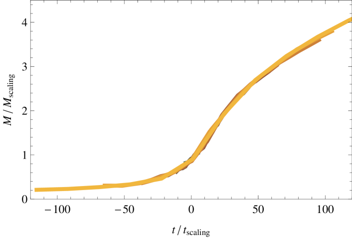
Figure 1: Scaling collapses for the magnetization and susceptibility using the scaling form given by the normal form Eqs.( 30 – 32). Simulations are done on a 4-d lattice using a Wolff algorithm for lattice sizes ranging from $L=4$ to $L=32$. Here $M_{\mathrm{scaling}}$ $=$ $L((W(yL^{1/D})+1))^{1/4}$ and $t_{\mathrm{scaling}}$ $=$ $L^{-2}(W(yL^{1/D})/(1/Du_{0}-1))^{1/3}((W(yL^{1/D})+1))^{-1/2}$. We find $u_{0}=0.4\pm 0.1$ for the 4-d nearest-neighbor hypercubic-lattice. An estimate of the error is given by estimating $u_{0}$ with a different choice of normal form which gives $u_{0}=0.5$.

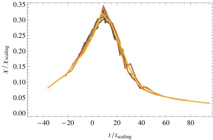
Figure 2: Scaling collapse for the susceptibility using the scaling form given by the normal form Eqs.( 30 – 32). Simulations are done on a 4-d lattice using a Wolff algorithm for lattice sizes ranging from $L=4$ to $L=32$. Here $\chi_{\mathrm{scaling}}$ $=$ $L^{2}((W(yL^{1/D})+1))^{1/2}$ and $t_{\mathrm{scaling}}$ $=$ $L^{-2}(W(yL^{1/D})/(1/Du_{0}-1))^{1/3}((W(yL^{1/D})+1))^{-1/2}$. We find $u_{0}=0.4$ for the 4-d nearest-neighbor hypercubic-lattice.

Before examining the full solution of Eqs. (30 – 32), we will first study the effect of each part of the RG flows. First, considering only the linear terms and coarse-graining until $t(\ell^{*})=1$, the free energy is given by $f\sim t^{2}$. This is the mean-field result and also the traditional scaling form that RG results take in the absence of nonlinear terms in the flow equations. Second, we include the resonance between the temperature and free energy eigenvalue, which leads to an irremovable $t^{2}$ term in the flow equation for the free energy. This term cannot be removed by analytic coordinate changes, and yields a $\log$ correction to the specific heat. Third, the irrelevant variable $u$ undergoes a transcritical bifurcation. Results in the hyper-normal form theory literature, as well as some articles in the high-energy theory literature sonoda ; magradze recognize that the simplest form that the equation can be brought into is Eq. 31. The solutions of Eqs.( 30 – 31) are $u(\ell)=1/(D(1+W(ye^{\ell/D})))$ and $t(\ell)=t_{0}e^{2\ell}(W(ye^{\ell/D})/(1/(Du_{0})-1))^{-A}$ where $y[u_{0}]$ is again a messy but explicit function: $y=(1/(Du_{0})-1)\exp(1/(Du_{0})-1)$. We show how to derive this in the supplementary material. The traditional log and log-log corrections are derived by expanding the $W$ function for large $\ell$.

Let us use this to derive the finite-size scaling form of the free energy. Early finite-size scaling work aktekin2001finite ; lai1990finite ; montvay1987numerical attempted scaling collapses with logs; recent work does not attempt collapses at all lundow2009critical . Finite-size scaling requires an equation for the magnetic field, $h$, given by $dh/d\ell=3h$. Explicit calculations show that the coefficient of the $hu$ term is zero (see below). The free energy is then a function of three scaling variables, $u(\ell)$, $t(\ell)$ and $h(\ell)$. It is given by

$$f(t_{0},u_{0}) =e^{-4\ell}f(t(\ell),u(\ell),h(\ell))$$

$$-W(ye^{\ell/D})^{-A}\left(\frac{W(ye^{\ell/D})^{-A}}{1-A}-\frac{1}{A}\right).$$ (33)

To get a finite size scaling form, we coarse grain until $\ell=\log L$, the system size. Note that $u(L)$ cannot just be ignored because it is a dangerous irrelevant variable. However we can account for it by taking the combination $t(L)/(u(L))^{1/2}$ and $h(L)/(u(L))^{1/4}$ as our scaling variables binder1985finite . The scaling form of the free energy then depends on $u_{0}$ which we do not have a way to change or set in the simulation. Instead, we treat $u_{0}$ as a fit parameter in the scaling form of the susceptibility:

$$\chi=L^{2}\left(W(yL^{\frac{1}{D}})+1\right)^{\frac{1}{2}}\Phi\left(t_{0}L^{2}\left(\frac{W(yL^{1/D})}{1/(Du_{0})-1}\right)^{-A}\right).$$ (34)

At the critical point $t=0$, the function $\Phi$ must be analytic for finite $L$ (since non-analyticity requires an infinite system size). $\Phi(0)$ is therefore a constant independent of $L$ and $u_{0}$ at $t=0$. Using this, $u_{0}$ may be estimated from $\chi$ at different values of $L$ by fitting to its predicted dependence $\chi\propto L^{2}(W(y[u_{0}]L^{1/D})+1)^{1/2}$ where $y[u_{0}]$ is defined above.

Figures 1–2 shows the scaling collapse of the magnetization and susceptibility. The magnetization is collapsed using the best-fit value of $u_{0}=0.4$. Though our collapses are not significantly better than the traditional logarithmic forms, the correct form of the singularity will be more apparent at larger values of $u_{0}$. This is because the $\log\log$ term which is the second term in the asymptotic expansion of the $W$ function is very small compared to the $\log$ except at large $u_{0}$ and small $L$. Changing the value of $u_{0}$ will require a model different from the nearest neighbor square lattice Ising model.

So far, we have been considering the effects of changing coordinates in the control variables on the predictions of the theory. Wegner wegner1974some had also considered changing coordinates in the degrees of freedom of the theory. These changes lead to ‘redundant’ variables, the corrections from which can be removed by coordinate changes. We discuss them in separate work. Here we merely note that they can be used to explain some features of the scaling, like the fact that the coefficient of the $hu$ term is zero.

V.1.1 Choice of normal form

There are certain choices we have made in our application of normal form theory. One is to keep the flow parameter $\ell$ unchanged. Some of the dynamical systems literature considers changing $\ell$ to depend on other parameters. This would be unusual since the coarse graining length would depend on the physical parameters but does not seem to be disallowed. We show in the supplementary material that this does not change the predictions for the 4-d Ising model.

Normal form theory makes a particular choice for what to do with the coefficients that can be changed by coordinate changes: it sets them equal to zero. In general, however, it is not clear that the best choice to make is to set them equal to zero. Consider the equation

$$\frac{du}{d\ell}=-u^{2}+Du^{3}$$ (35)

which, as we saw, has the solution $u(\ell)=1/(D(1+W(ye^{\ell/D})))$. Here, $y=(1/(Du_{0})-1)\exp(1/(Du_{0})-1)$. Note that $u_{0}>0$ as a requirement for the stability of the free energy. If $u_{0}<1/D$, then $y>0$, and if $u_{0}\leq 1/D$, $y\leq 0$. Hence, the domain of attraction of the fixed point at $u_{0}=0$ has a length $1/D$. If we have a system where $u_{0}>1/D$, then this will lead to $u(\ell)\rightarrow\infty$ in a finite coarse graining length. This is reflected in the branch cut of the $W$ function at $-1/e$. In the context of high energy physics, some have tried to find deep meaning in this pole magradze .

However, for scaling purposes, we generally prefer a choice of coordinates for which there is no such unphysical behavior. One natural choice is to instead use the equations

$$\frac{du}{d\ell}=-\frac{u^{2}}{1+Du}.$$ (36)

For small $u$, this has the same behavior as Eq. 35. However, the behavior at large $u$ is now well behaved. The solution of this equation is

$$u(\ell)=\frac{1}{DW(e^{\ell/D}1/(Du_{0})e^{1/(Du_{0})})},$$ (37)

which is in fact somewhat simpler that the solution to Eq.( 35). Scaling collapses with this choice of normal form for the susceptibility are shown in the case of the Ising model in Figure 3. Better numerics are needed to tell if this choice of normal form is really useful. It turns out that this form has been implicitly used before in the Random Field Ising model as we show explicitly in the next section.

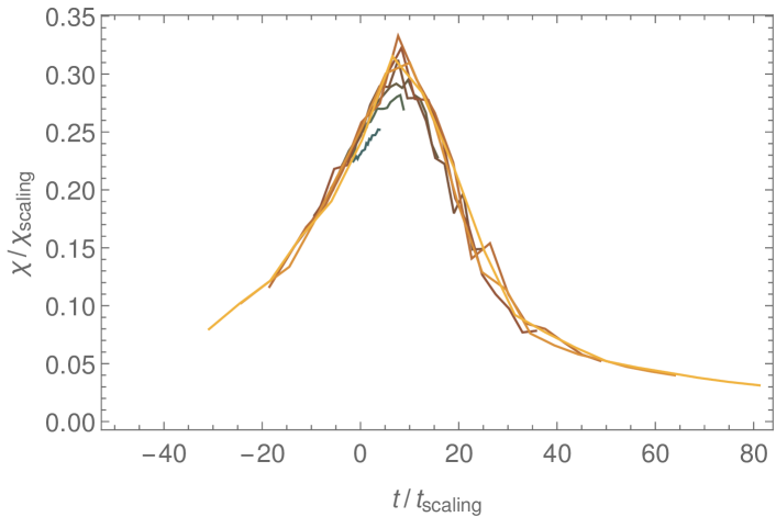
Figure 3: Scaling collapse for the susceptibility using the scaling form given by a different choice of normal form derived from Eq.( 36). Simulations are done on a 4-d lattice using a Wolff algorithm for lattice sizes ranging from $L=4$ to $L=32$. Here $\chi_{\mathrm{scaling}}$ $=$ $L^{2}((W(yL^{1/D}))^{1/2}$ and $t_{\mathrm{scaling}}$ $=$ $L^{-2}(W(yL^{1/D}))^{-1/6}/(1/Du_{0}))^{1/3}\exp(1/(3W(yL^{1/D})))$ with $y=1/(Du_{0})e^{1/(Du_{0})}$. We find $u_{0}=0.5$ for the 4-d nearest-neighbor hypercubic-lattice using this method.

V.2 Random Field Ising model

Finding critical exponents for the random field Ising model has been a longstanding challenge in physics. Some initial results used supersymmetry to prove an equivalence of the Random Field Ising model in dimensions $d+2$ with the Ising model in dimensions $d$ parisi1979random ; de2006random . It was later shown that the lower critical dimension of the Random Field Ising model is not $3$ (as would be expected from such a correspondence) but rather $2$ imbrie1984lower . The upper critical dimension is 6. Here, we will look at the scaling behavior of the Random Field Ising model at its lower critical dimension, $d=2$.

Consider a spin system with a random field.

$$\mathcal{H}=-\sum_{\langle ij\rangle}Js_{i}s_{j}+\sum_{i}h_{i}s_{i},$$ (38)

where, $J$ is the nearest neighbor coupling and $h_{i}$ is a random field chosen from a Gaussian distribution with width $r$. A phenomenological theory for the RG was formulated by Bray and Moore Bray85 . It turns out to be useful to define a quantity $w=r/J$. Then, using heuristic arguments on the stability of domain walls, they derive

$$\frac{dw}{d\ell}=-\epsilon/2w+Aw^{3},$$ (39)

with $\epsilon=d-2$, and $d$ is the dimension. Note that the flow equations have a symmetry under $w\rightarrow-w$ because the physics is invariant under $r\rightarrow-r$ about the critical point at $r=0$. This is an example of a pitchfork bifurcation. Bray and Moore argue for this scaling form by looking at the scaling of $r$ and $J$ separately. The scaling of $J$ is given by looking at the energy of a domain wall of size $b^{d}$. The energy of the domain wall is proportional to $b^{d-1}$. By considering the cost of roughening the domain wall because of the presence of random fields, which goes as $r^{2}$, they are able to derive the next term in the equation for $J$ which is now

$$\frac{dJ}{d\ell}=(d-1)J+Dw^{2}J+\mathcal{O}(w^{4}).$$ (40)

For the random field $r$, the energy of a region of size $b^{d}$ is proportional to $b^{d/2}$. Any corrections requires forming a domain of ‘wrong spins’ which, being akin to a barrier crossing problem, is exponentially suppressed. Hence the equation for $r$ is given by

$$\frac{dr}{d\ell}=\frac{d}{2}r$$ (41)

with exponentially small corrections. These two equations together can be used to derive Eq.( 39). Bray and Moore conjecture that Eq.( 41( holds exactly to all orders in $w$ (up to exponential corrections). However, it is possible for Eq. (40) to have higher order terms in $w$ and thus Eq.( 39) is only correct to order $w^{5}$. Integrating Eq.( 39), we get $\ell\sim-1/(2Aw^{2})+1/(2Aw_{0}^{2})$. This implies that the correlation length is

$$\xi\sim e^{1/(2Aw_{0}^{2})}.$$ (42)

For finite size systems, the system size $L\sim\exp(1/(2Aw_{0}^{2})$. Meinke and Middleton Meinke05 showed that their finite size data was much better fit by a function of the form $w_{0}^{-2y}\exp(C/w_{0}^{2})$ where $C$ is a constant they fit to ($C=\Delta_{0}$ in their notation) and $y$ = 1.07. We will show that this prediction is consistent with the results of normal form theory.

As we have already argued, there is no reason Eq.( 39) is true to all orders in $w$. Indeed the, normal form prediction for the flow equations can be derived in a straightforward way. Consider adding a term $A_{n}w^{n}$ to Eq.( 39) at $\epsilon=0$. This is a resonance and cannot be removed usually under normal form theory. Suppose we make a change of coordinates $w=\tilde{w}+a_{n}\tilde{w}^{n-2}$. Then, to order $\mathcal{O}(\tilde{w}^{n})$, we get

$$\frac{d\tilde{w}}{d\ell}=A\tilde{w}^{3}+(3Aa_{n}-Aa_{n}(n-2)+A_{n})\tilde{w}^{n}+\mathcal{O}(\tilde{w}^{n+1}).$$ (43)

We can set the coefficient of $\tilde{w}^{n}=0$ if we use $a_{n}=A_{n}/((n-5)A)$. This procedure fails for $n=5$ but works for all $n>5$. Hence, the normal form of the equilibrium RFIM is given by

$$\frac{d\tilde{w}}{d\ell}=\tilde{w}^{3}-D\tilde{w}^{5}.$$ (44)

As before, we have used the freedom to rescale $w$ to set the coefficient of the $\tilde{w}^{3}$ term to 1.

The solution of this equation gives us an expression for the correlation length

$$\xi\sim(1/w^{2}-D)^{D/2}e^{1/w^{2}}.$$ (45)

This scaling form could explain the data in Meinke and Middleton with $D$ as a fit parameter. Notice that for this to work, $D$ must be positive. However, this solution has the strange property that the correlation length goes to $0$ for $w^{2}=1/D$. If $w^{2}>1/D$, $w^{2}(l)$ decreases till it reaches $1/D$. If $w^{2}<1/D$, it increases till it reaches $1/D$. As in the 4-d Ising model, it may be more useful to consider instead the flow equation

$$\frac{d\tilde{w}}{d\ell}=\frac{\tilde{w}^{3}}{1+D\tilde{w}^{2}}.$$ (46)

This gives the scaling form

$$\xi\sim e^{1/(2w^{2})}(w^{2})^{-D/2}.$$ (47)

This is exactly consistent with the scaling form Meinke and Middleton use to collapse their data. Their data would predict the universal value for $D=2.14$ . Any system in the same universality class should see a value of $D$ consistent with this value. However, different values of $D$ would correspond to different universality families within the same class. We now turn to discussing the XY model before returning to the Ising model in dimensions 3, 2, and 1.

V.3 2-D XY Model

The 2-d XY model is a remarkable system for several reasons. It was the site of recently celebrated insight into the connection between ground-state topology and phase transitions kosterlitz2017nobel . Thermodynamic quantities have essential singularities at its phase transition, not ordinary power laws, and their derivatives remain continuous to arbitrary order, making its phase transition infinite order berezinskii1970destroying ; kosterlitz1973ordering ; kosterlitz1974critical . This is related the fact that its RG flow equations are inherently nonlinear: they have no relevant and two marginal state variables and the procedure laid out by (11) for removing higher order terms from the flow equations contributes nothing to their simplification.

The XY model is usually posed as ferromagnetically interacting planar spins. Its partition function is exactly equivalent to the product of a trivial Gaussian model—corresponding to spin wave degrees of freedom—with a neutral Coulomb gas—corresponding to the interaction of spin vortices knops1977exact . The latter component contains the interesting critical behavior, which is characterized by these vortices going through an unbinding transition. The flow equations for a Coulomb gas in dimension $d$ are given by

$$dK/dl =-K(\tfrac{1}{4}Ky^{2}+d-2)+\cdots$$ (48)

$$dy/dl =-y(K-d)+\cdots,$$ (49)

where $K\sim T^{-1}$ and $y$ is the fugacity of the vortices kosterlitz1977d , which for an XY model is a function of temperature and cannot be tuned independently but is a free parameter in other equivalent models, e.g., the Coulomb gas itself. For $d>2$ there is no phase transition in this system, and for $d<2$ a nontrivial unstable fixed point appears and there is a phase transition in the hyperbolic universality family. It is worth noting that these flow equations do not describe the XY model for any dimension besides $d=2$; 2 is the upper critical dimension of the Coulomb gas and these flow equations, while it is the lower critical dimension for the XY model. At $d=2$ the flow equations undergo a novel bifurcation: there appears a line of stable fixed points at $y=0$ for all $K>2$, terminating at $K=2$. This termination is the Berezinskii–Kosterlitz–Thouless (BKT) critical point. The flow equation near this point with $x=K-2$ is

$$dx/dl =-y^{2}+\cdots$$ (50)

$$dy/dl =-xy+\cdots.$$ (51)

These flow equations are zero to linear order and have zero Jacobian at the fixed point.

In principle arbitrary higher-order terms in these equations exist, but there are several constraints on their form. There is a symmetry $y\to-y$ in the partition function arising from the neutrality condition—$y$ enters the partition function in factors of $y^{-\sum_{r}n_{r}^{2}}$ for $\sum_{r}n_{r}=0$—which implies that $dx/dl$ be even in $y$ and $dy/dl$ be odd. In addition, when the fugacity is zero the model is trivial and $x$ cannot flow, meaning that $dx/dl$ must only have terms proportional to $y$. Having applied these constraints, the simplest normal form has been proven by induction in polynomial order (Appendix A of pelissetto2013renormalization ) to take the form

$$d\tilde{x}/dl =-\tilde{y}^{2}-b_{0}\tilde{x}\tilde{y}^{2}-b_{1}\tilde{x}^{3}\tilde{y}^{2}+\cdots$$ (52)

$$=-\tilde{y}^{2}\big{(}1+\tilde{x}f(\tilde{x}^{2})\big{)}$$ (53)

$$d\tilde{y}/dl =-\tilde{x}\tilde{y}.$$ (54)

For the BKT point in the sine–Gordon model, which is thought to display to the same universality as the XY model, it is known that $b_{0}=3/2$ balog2000intrinsic ; pelissetto2013renormalization . An infinite number of coefficients remain, represented here in the form of the Taylor coefficients of an analytic function $f(x^{2})$. These numbers are universal in the sense that there is no redefinition of $\tilde{x}$ and $\tilde{y}$ such that the flow equations take on the form above and contain different coefficient values. Unlike those in the previous sections, this bifurcation does not have a named classification as far as the authors know.

A constant of the RG flow can be found by integrating these forms. First, dividing the equations (54) by (53) (and dropping the tildes), we find

$$\frac{dy}{dl}\bigg{/}\frac{dx}{dl}=\frac{x}{y(1+xf(x^{2}))},$$ (55)

which separates into

$$y\frac{dy}{dl}=\frac{x}{1+xf(x^{2})}\frac{dx}{dl}.$$ (56)

Integrating both sides and choosing $l_{0}$ such that $x(l_{0})=0$, we find

$$\frac{1}{2} \big{(}y(l)^{2}-y(l_{0})^{2}\big{)}=\int_{y(l_{0})}^{y(l)}y\,dy=\int_{l_{0}}^{l}y\frac{dy}{dl}dl$$ (57)

$$=\int_{l_{0}}^{l}\frac{x}{1+xf(x^{2})}\frac{dx}{dl}dl=\int_{0}^{x(l)}\frac{x}{1+xf(x^{2})}dx.$$ (58)

It follows that

$$y(l_{0})^{2} =y(l)^{2}-2\int_{0}^{x(l)}\frac{x}{1+xf(x^{2})}dx$$ (59)

$$=y(l)^{2}-x(l)^{2}+\frac{2}{3}b_{0}x(l)^{3}-\frac{1}{2}b_{0}x(l)^{4}$$ (60)

$$\hskip 40.00006pt+\frac{2}{5}(b_{0}^{3}+b_{1})x(l)^{5}+O(x(l)^{6})$$ (61)

is a constant of the flow. The expansion of the integral can be taken to arbitrary order with ordinary computer algebra software. The finite-size behavior of the flow is rather complicated and doesn’t yield closed form results, details can be found in pelissetto2013renormalization .

The XY model and other infinite-order transitions are usually characterized by the anomalous exponent $\sigma$ parametrizing the essential singularity in the correlation length,

$$\xi\sim e^{at^{-\sigma}},$$ (62)

which for the BKT transition is $\sigma=1/2$ kosterlitz1974critical . Conformal field theory predicts the presence of infinitely many models with this anomalous exponent ginsparg1988applied . The value of $\sigma$ been shown to be fixed by the quadratic-order truncation of the system’s flow equation, independent of any higher-order terms itoi1999renormalization . There are six possible quadratic-order terms in flow equations with two variables. Of these, two can be removed by linear transformations of the two variables. Two more can be set to 1 by rescaling the variables. Hence, there are two parameters at quadratic order which determine the universality family that the system belongs to, and infinite number of subsequent terms which determine the universality class. Giving a full classification of possibilities is beyond the scope of this paper but we give some examples below.

For instance, when the requirement of symmetry under $y\to-y$ is lifted, the flow equations can no longer be brought to the form Eqs. (53) and (54); though the simplest form that results isn’t yet known, it is certainly different from the symmetric case, a fact that can be found by simply trying to eliminate the nonsymmetric cubic terms. In such a case the codimension of the bifurcation would likely be different, corresponding to the fact that no a priori reason exists for the vanishing of the term linear in $y$ in $dx/dl$. Such linear terms would change the universality family. Among the infinite collection of BKT-like conformal theories—including the many physical models identified as having a BKT-like transition because their behavior resembles Eq. (62), like percolation in grown networks callaway2001randomly ; dorogovtsev2001anomalous . These may already be examples of models with $\sigma=1/2$ but belonging to another universality class. It could also be the case that all BKT-like transitions are in fact members of the same universality family and class.

Other universality classes and families definitely do exist, characterized by novel values for $\sigma$. The level-1 $\mathrm{SU}(N)$ Wess–Zumino–Witten model has been found to be characterized by $\sigma=N/(N+2)$ itoi1997extended . Dislocated-mediated melting alone has produced a melange of anomalous exponents, with $\sigma=1/2$, $\sigma=2/5$, and $\sigma=0.369\,63\ldots$ depending on precise specification of the model and the lattice geometry nelson1979dislocation ; young1979melting . Topological transitions in systems whose vortices are non-Abelian produce several series of $\sigma$ values dependent on particular symmetry bulgadaev1999berezinskii . Each value of $\sigma$ indicates either a different universality family or merely a different class within the same family depending on how it affects the terms at quadratic order. A classification of possible bifurcations and corresponding simplest normal forms is in order for flow equations whose leading order is quadratic, and whose expansions are constrained or not by various symmetries. This would be the first step in developing techniques for distinguishing between universality classes and families of this type using experimental or simulation data.

V.4 3-d Ising model

There is a sense in which the Ising model is simplest in 3 dimensions because it is part of the hyperbolic universality family. It is also the first natural application of the $\epsilon$ expansion. The transcritical bifurcation at 4 dimensions leads to an exchange of stabilities of the Gaussian fixed point and the Wilson-Fisher fixed point at a non-zero value of $u=u^{*}$. About this Wilson-Fisher fixed point, the flow equations of the 3-d Ising model are in the hyperbolic universality class with linear coefficients which define the Ising universality class.

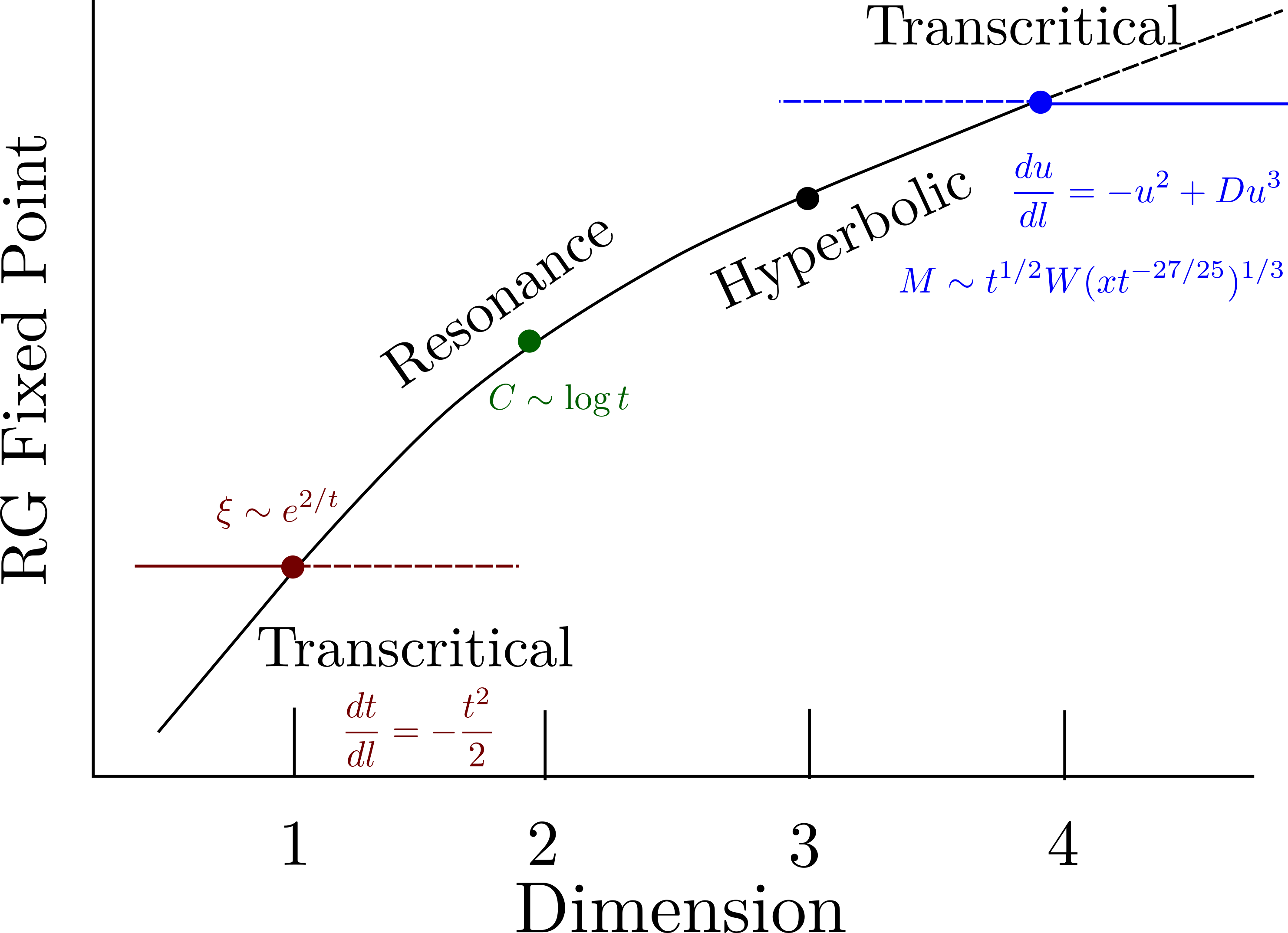
Figure 4: Fixed points as a function of dimension in the Ising model. There is a transcritical bifurcation in both 4 and 1 dimensions, leading to $W$ functions and exponential correlation lengths respectively. The fixed point in 3 d is hyperbolic and the flow can be linearized. The fixed point in 2 d has a resonance which leads to a logarithmic specific heat. The challenge is to find a scaling form which interpolates between dimensions giving the correct behavior in all of these dimensions.

However, another approach is to consider the scaling form as a function of the dimension $\epsilon$ in a way that is well defined even at $\epsilon=0$. Doing this, naturally requires us to keep nonlinear terms in the equation because we already know that the 4-d Ising model has nonlinear terms in its flow equations.

We want to write the flow equations about the 3-d fixed point but keep the nonlinear terms required for the scaling form to have the correct limiting behavior in 2-d and in 4-d. We can write the normal form of the flow equations as

$${d\tilde{t}}/{d\ell} =\lambda_{t}\tilde{t}-A\tilde{u}\tilde{t},$$ (63)

$${d\tilde{u}}/{d\ell} =\lambda_{u}\tilde{u}-\tilde{u}^{2}+D\tilde{u}^{3},$$ (64)

$${d\tilde{f}}/{d\ell} =d\tilde{f}-{\tilde{t}}^{2},$$ (65)

$${d\tilde{h}}/{d\ell} =\lambda_{h}h.$$ (66)

We have included the nonlinear terms in $u$ required for the correct scaling behavior and the resonance between the temperature and the free energy. As usual, we switch notation to $t$, $h$ and $u$ with the understanding that they are different from the normal form variables by analytic corrections. Let us look at the scaling variable formed with $t$ and $u$ which can be obtained by solving

$$\frac{d\tilde{t}}{d\tilde{u}}=(\lambda_{t}\tilde{t}-A\tilde{u}\tilde{t})/(\lambda_{u}\tilde{u}-\tilde{u}^{2}+D\tilde{u}^{3}).$$ (67)

The solution of this equation gives the scaling variable

$$t(u)^{-\frac{\lambda_{t}}{Du_{1}u_{2}}}(u-u_{1})^{-\frac{(\lambda_{t}-Au_{1})}{Du_{1}(u_{1}-u_{2})}}(u-u_{2})^{\frac{\lambda_{u}-Au_{2}}{D(u_{2}-u_{1})u_{2}}}=\textrm{const}$$ (68)

where $u_{1}$ and $u_{2}$ are the two non-zero roots of the denominator on the r.h.s of Eq.67 which to first order in $\lambda_{u}$ are given by $u_{1}=\lambda_{u}$ and $u_{2}=1/D-\lambda_{u}$. The form of the scaling variable is interesting, it is essentially given by a product of the linearized scaling variables at the three fixed points that the equation has. Taking the limit $\epsilon\rightarrow 0$, we get

$$te^{-2/u}u^{2D-A}(1-Du)^{A-2D}=\textrm{const}$$ (69)

which is the right scaling variable in $4$-d. We have not yet been able to obtain an analytical form for the scaling variable involving $t$ and $h$. This is because the equation for $u(l)$ does not seem to have a closed-form solution here (unlike the 4-d case). Nevertheless, we are motivated by an attempt to create scaling variables which interpolate between different dimensions and have the correct scaling behavior in many dimensions going down from $4$ to $1$. Once the full scaling variables are written down, a first test would be to see if these scaling variables do better collapsing the numerical data in 3-d.

V.5 1-d Ising model

The 1-d Ising model is somewhat different because it is the lower critical dimension and does not have a phase transition. The 1-d Ising model has an exact solution which can be obtained by using transfer matrices. The partition function can be written as the trace of a transfer matrix $\mathcal{T}^{N}$ where $N$ is the number of spins in the system. The matrix $\mathcal{T}_{ij}=e^{-\beta\mathcal{H}(s_{i}s_{j})}$. Coarse graining here can be done by a well-defined procedure, the coarse grained transfer matrix is defined as $\tilde{\mathcal{T}}=\mathcal{T}^{b}$ where $b$ is the coarse graining length scale. Defining $\ell=\log b$ and expanding for $b$ close to 1, we can get flow equations for the temperature $T$

$$\frac{dT}{d\ell}=-\frac{T^{2}}{2}\sinh\left(\frac{2}{T}\right)\log\left(\tanh\left(\frac{1}{T}\right)\right).$$ (70)

This is different from the flow equations we have considered so far because of the presence of non-analytic terms in the flow. The non-analytic term which multiplies the $T^{2}$ term is $=-1$ at $T=0$. So, this equation corresponds to a transcritical bifurcation

$$\frac{dT}{d\ell}=\frac{T^{2}}{2}+...$$ (71)

where the additional terms are non-analytic at $T=0$. This can be used to derive a correlation length $\chi\sim\exp(2/T)$. To interpret the flow further, consider the change of coordinates $\kappa=\exp(-2/T)$. In these variables, the flow is

$$\frac{d\kappa}{d\ell}=(\kappa^{2}-1)\log\left(\frac{1-\kappa}{\kappa+1}\right).$$ (72)

Evidently, the flow is analytic in this variable. Solving the full flow Eq.( 70) gives $\chi\sim-1/(\log\tanh(1/T))$.

For non-zero $\epsilon$, this argument is usually extended in what is called a Migdal-Kadanoff procedure for doing RG kadanoff1976notes ; chaikin1995principles . The flow equations are identical except for the presence of a $-\epsilon T$ term which serves as the bifurcation parameter. The $1+\epsilon$ expansion can be summed completely because the flow equation is known to all orders. It does not yield very accurate critical exponents though it gives the exact value of the critical temperature in 2-d (because it respects duality symmetry). Several people have improved the expansion martinelli1981systematical ; bruce1981droplet .

The presence of non-analytic terms in the flow equations complicates the application of normal form theory. We will come back to it when discussing Legendre transform of flow equations.

V.6 2-d Ising model

The 2-d Ising model is a particularly nice example because it has an exact solution in the absence of a magnetic field. All predictions then can be compared to the exact solution. Surprisingly, despite the known exact solution, the scaling behavior of the 2-d Ising model is still not completely understood. A full discussion of the 2-d Ising model will be given in separate work Clement18 . Here, we give a brief summary of the issues involved.

The only variable required to describe the 2-d Ising model in the absence of a field is the temperature $t$. The linear eigenvalues of the free energy and the temperature are $2$ and $1$ respectively. The normal form of the flow equations can be written as

$$\frac{d\tilde{f}}{d\ell} =2\tilde{f}-\tilde{t}^{2},$$ (73)

$$\frac{d\tilde{t}}{d\ell} =\tilde{t}.$$ (74)

We have used the fact that the only term which cannot be removed by traditional normal form analysis is the resonance $t^{2}$. In fact, it cannot be removed by any analytic change of variables. We have also used the freedom to rescale $t$ to set the coefficient of the resonance equal to -1 . The solution to this can be written as $\tilde{t}=\tilde{t}_{0}e^{\ell}$ and the free energy

$$\tilde{f}(\tilde{t}_{0},\ell)=e^{-2\ell}\tilde{f}(\tilde{t}_{0}e^{\ell})-\tilde{t}_{0}^{2}\ell.$$ (75)

Coarse graining until $\tilde{t}(\ell)=1$ or $l=-\log(\tilde{t}_{0})$, we get

$$\tilde{f}(\tilde{t}_{0})=\tilde{t}_{0}^{2}\tilde{f}(1)+\tilde{t}_{0}^{2}\log\tilde{t}_{0}.$$ (76)

Now, the normal form variable $\tilde{t}_{0}$ is some analytic function of the physical variable $t_{0}$. It is linear to first order in $t_{0}$. Hence, we can write it as $\tilde{t}_{0}=t_{0}(1+c(t_{0}))$ where $c$ is some analytic function. Then, we can expand

$$\tilde{f}(t_{0}) =t_{0}^{2}(1+c(t_{0}))^{2}f(1)+t_{0}^{2}(1+c(t_{0}))^{2}\log t_{0}(1+c(t_{0})),$$ (77)

$$=t_{0}^{2}(1+c(t_{0}))^{2}f(1)+t_{0}^{2}(1+c(t_{0}))^{2}\log(1+c(t_{0}))+t_{0}^{2}(1+c(t_{0}))^{2}\log t_{0},$$ (78)

$$=a(t_{0})+b(t_{0})\log t_{0}$$ (79)

where both $a(t_{0})$ and $b(t_{0})$ are some analytic functions of $t_{0}$. Meanwhile any change of coordinates which adds an analytic function of $t_{0}$ to $\tilde{f}$ can be absorbed in the definition of $a(t_{0})$. Hence, we can write the final most general form of the free energy of the 2-d Ising model as $f=a(t_{0})+b(t_{0})\log t_{0}$. Indeed, the exact solution of the 2-d Ising model can be written in this form caselle2002irrelevant .

While the basic solution of the 2-d Ising model is simple, some challenges still remain. The scaling form in the presence of other variables (like the magnetic field and other irrelevant variables) which has so far only been conjectured aharony1983nonlinear ; caselle2002irrelevant naturally follows from an application of normal form theory. It is given simply by including other variables in the argument of the free energy in Eq.( 75) before coarse graining till $t(\ell)=1$. Irrelevant variables are the source of singular corrections to scaling. An interesting unresolved issue is the presence of higher powers of logarithms in the susceptibility which are not found in the free energy orrick2001susceptibility ; chan2011ising . This is usually attributed to the presence of irrelevant variables. Here it is possible to show that the irrelevant variables which are derived from conformal field theory caselle2002irrelevant would in fact lead to higher powers of logarithms in the free energy which are not observed. Hence, they cannot explain the higher powers of logarithms in the susceptibility. It is possible that there are other irrelevant variables in the 2-d square lattice nearest neighbor Ising model with a field which are not predicted by conformal field theory but can capture the higher powers of logarithms in the susceptibility, as they turn on with a field.

The logarithm due to the resonance in the 2-d Ising model is most apparent in the specific heat. It is easy to derive the flow equations for the inverse specific heat which have the form

$$\frac{dC^{-1}}{d\ell}=2C^{-2},$$ (80)

and has a transcritical bifurcation in two dimensions. This raises a question, is it legitimate to talk about a bifurcation in two dimensions for the Ising model if it happens in the space of results rather than the space of control variables? Intriguingly, though perhaps unrelated, a bifurcation has been observed in 2 dimensions using methods of conformal bootstrap golden2015no ; el2014conformal . In thermodynamics, a natural framework which interchanges between results and control parameters is given by Legendre transforms. However, the flow equations for the Legendre transformed coordinates generically have non-analyticities in them. We suspect that the variable $t$ (and $h$ etc.) is uniquely specified as the correct variable for RG. It is possible that it is more natural to consider removing degrees of freedom in the canonical ensemble ($t$ and $f$), then in a microcanonical one ($E$ and $S$) . A fuller discussion will be given in forthcoming work Clement18 .

VI Conclusion

We have shown how normal form theory leads to systematic procedure for handling the singularity in RG flows. The concept of universality families broadens the notion of a universality class and we have elucidated it with several different examples. We have focused on getting a precise handle on the singularity at the critical point. However, normal form theory also gives an elegant way to fit corrections to scaling. Interestingly, even the scaling of the 2-d Ising model which has an exact solution has some unresolved mysteries which we are exploring. It is possible that interpolating between dimensions in a way that captures the correct singularities can improve scaling collapses in all dimensions. Finally, we are exploring the application of our methods to systems like jamming in 2-d goodrich2014jamming , where logarithmic corrections are observed but no renormalization-group theory is available. In general, we expect this fruitful confluence of dynamical systems theory and the renormalization group will not only clarify and illuminate previously known technical calculations, but will also facilitate quantitative analysis of experimental and theoretical systems farther from their critical points and before the underlying field theory is well understood.

VII Acknowledgements

We thank Tom Lubensky, Andrea Liu, John Guckenheimer, Randall Kamien and Cameron Duncan for useful conversations. AR, CBC, LXH, JPK, DBL and JPS were supported by the National Science Foundation through Grant No. NSF DMR-1719490. LXH was supported by a fellowship from Cornell University. DZR was supported by the Bethe/KIC Fellowship and the National Science Foundation through Grant No. NSF DMR-1308089.

References

- [1] Benjamin B Machta, Sarah L Veatch, and James P Sethna. Critical Casimir forces in cellular membranes. Physical review letters, 109(13):138101, 2012.
- [2] Léonie Canet, Bertrand Delamotte, and Nicolás Wschebor. Fully developed isotropic turbulence: Nonperturbative renormalization group formalism and fixed-point solution. Physical Review E, 93(6):063101, 2016.
- [3] Ashivni Shekhawat, Stefano Zapperi, and James P Sethna. From damage percolation to crack nucleation through finite size criticality. Physical review letters, 110(18):185505, 2013.
- [4] Yong S Chen, Woosong Choi, Stefanos Papanikolaou, Matthew Bierbaum, and James P Sethna. Scaling theory of continuum dislocation dynamics in three dimensions: Self-organized fractal pattern formation. International Journal of Plasticity, 46:94–129, 2013.
- [5] Ernst Ising. Beitrag zur theorie des ferromagnetismus. Zeitschrift für Physik A Hadrons and Nuclei, 31(1):253–258, 1925.
- [6] Jesús Salas. Exact finite-size-scaling corrections to the critical two-dimensional Ising model on a torus: Ii. Triangular and hexagonal lattices. Journal of Physics A: Mathematical and General, 35(8):1833, 2002.
- [7] AI Larkin and E Khmel’nitskii. Phase transition in uniaxial ferroelectrics. WORLD SCIENTIFIC SERIES IN 20TH CENTURY PHYSICS, 11:43–48, 1995.
- [8] Franz J Wegner and Eberhard K Riedel. Logarithmic corrections to the molecular-field behavior of critical and tricritical systems. Physical Review B, 7(1):248, 1973.
- [9] J M Kosterlitz and D J Thouless. Ordering, metastability and phase transitions in two-dimensional systems. Journal of Physics C: Solid State Physics, 6(7):1181, 1973.
- [10] H. W. Diehl and E. Eisenriegler. Walks, polymers, and other tricritical systems in the presence of walls or surfaces. EPL (Europhysics Letters), 4(6):709, 1987.
- [11] E. Eisenriegler and H. W. Diehl. Surface critical behavior of tricritical systems. Phys. Rev. B, 37:5257–5273, Apr 1988.
- [12] Daniel Dantchev, H. W. Diehl, and Daniel Grüneberg. Excess free energy and Casimir forces in systems with long-range interactions of van der Waals type: General considerations and exact spherical-model results. Phys. Rev. E, 73:016131, Jan 2006.
- [13] Björn Ahrens and Alexander K. Hartmann. Critical behavior of the random-field Ising model at and beyond the upper critical dimension. Phys. Rev. B, 83:014205, Jan 2011.
- [14] H. W. Diehl, Daniel Grüneberg, Martin Hasenbusch, Alfred Hucht, Sergei B. Rutkevich, and Felix M. Schmidt. Exact thermodynamic Casimir forces for an interacting three-dimensional model system in film geometry with free surfaces. EPL (Europhysics Letters), 100(1):10004, 2012.
- [15] H. W. Diehl, Daniel Grüneberg, Martin Hasenbusch, Alfred Hucht, Sergei B. Rutkevich, and Felix M. Schmidt. Large- approach to thermodynamic Casimir effects in slabs with free surfaces. Phys. Rev. E, 89:062123, Jun 2014.
- [16] Jesús Salas and Alan D. Sokal. Logarithmic corrections and finite-size scaling in the two-dimensional 4-state Potts model. Journal of Statistical Physics, 88(3):567–615, 1997.
- [17] Lev N. Shchur, Bertrand Berche, and Paolo Butera. Numerical revision of the universal amplitude ratios for the two-dimensional 4-state Potts model. Nuclear Physics B, 811(3):491 – 518, 2009.
- [18] B Berche, P Butera, and L N Shchur. The two-dimensional 4-state Potts model in a magnetic field. Journal of Physics A: Mathematical and Theoretical, 46(9):095001, 2013.
- [19] Olaf Stenull and Hans-Karl Janssen. Logarithmic corrections to scaling in critical percolation and random resistor networks. Phys. Rev. E, 68:036129, Sep 2003.
- [20] James Murdock. Normal forms and unfoldings for local dynamical systems. Springer Science & Business Media, 2006.
- [21] Stephen Wiggins. Introduction to applied nonlinear dynamical systems and chaos, volume 2. Springer Science & Business Media, 2003.
- [22] G Toulouse and M Kléman. Principles of a classification of defects in ordered media. Journal de Physique Lettres, 37(6):149–151, 1976.
- [23] Dominik Rogula. Large deformations of crystals, homotopy, and defects. In Trends in applications of pure mathematics to mechanics, pages 311–331, 1976.
- [24] N. D. Mermin. The topological theory of defects in ordered media. Reviews of Modern Physics, 51:591–648, 1979.
- [25] Paul M. Goldbart and Randall D. Kamien. Tying it all together. Physics Today, 72:46, 2019.
- [26] Franz J Wegner. Corrections to scaling laws. Physical Review B, 5(11):4529, 1972.
- [27] J. H. Meinke and A. A. Middleton. Linking physics and algorithms in the random-field Ising model. eprint arXiv:cond-mat/0502471, February 2005.
- [28] H Sonoda. Solving renormalization group equations with the Lambert W function. Physical Review D, 87(8):085023, 2013.
- [29] BA Magradze. An analytic approach to perturbative QCD. International Journal of Modern Physics A, 15(17):2715–2733, 2000.
- [30] Andrea Pelissetto and Ettore Vicari. Renormalization-group flow and asymptotic behaviors at the Berezinskii-Kosterlitz-Thouless transitions. Physical Review E, 87(3):032105, 2013.
- [31] Mustansir Barma and Michael E Fisher. Corrections to scaling and crossover in two-dimensional Ising and scalar-spin systems. Physical Review Letters, 53(20):1935, 1984.
- [32] Mustansir Barma and Michael E. Fisher. Two-dimensional Ising-like systems: Corrections to scaling in the Klauder and double-Gaussian models. Phys. Rev. B, 31:5954–5975, May 1985.
- [33] Martin Hasenbusch, Francesco Parisen Toldin, Andrea Pelissetto, and Ettore Vicari. Universal dependence on disorder of two-dimensional randomly diluted and random-bondj ising models. Physical Review E, 78(1):011110, 2008.
- [34] Lorien Hayden, Archishman Raju, and James P Sethna. Nonlinear scaling theory of the two-dimensional non-equilibrium random-field ising model. forthcoming.
- [35] David R. Nelson. Liquids and glasse in spaces of incommensurate curvature. Physical Review Letters, 50:982, 1983.
- [36] Archishman Raju and James P Sethna. Reexamining the renormalization group: Period doubling onset of chaos. arXiv preprint arXiv:1807.09517, 2018.
- [37] Carl P Goodrich, Simon Dagois-Bohy, Brian P Tighe, Martin van Hecke, Andrea J Liu, and Sidney R Nagel. Jamming in finite systems: Stability, anisotropy, fluctuations, and scaling. Physical Review E, 90(2):022138, 2014.
- [38] RE Lee DeVille, Anthony Harkin, Matt Holzer, Krešimir Josić, and Tasso J Kaper. Analysis of a renormalization group method and normal form theory for perturbed ordinary differential equations. Physica D: Nonlinear Phenomena, 237(8):1029–1052, 2008.
- [39] Shin-Ichiro Ei, Kazuyuki Fujii, and Teiji Kunihiro. Renormalization-group method for reduction of evolution equations; invariant manifolds and envelopes. Annals of Physics, 280(2):236–298, 2000.
- [40] Mohammed Ziane. On a certain renormalization group method. Journal of Mathematical Physics, 41(5):3290–3299, 2000.
- [41] Henri Poincaré. Les nouvelles méthodes de la mécanique céleste. Gauthier-Villars, Paris, I-III, 1899.
- [42] Alain Chenciner. Poincaré and the three-body problem. In Henri Poincaré, 1912–2012, pages 51–149. Springer, 2015.
- [43] John Cardy. Scaling and renormalization in statistical physics, volume 5. Cambridge university press, 1996.
- [44] James Murdock. Hypernormal form theory: foundations and algorithms. Journal of Differential Equations, 205(2):424–465, 2004.
- [45] Pei Yu and AYT Leung. The simplest normal form and its application to bifurcation control. Chaos, Solitons & Fractals, 33(3):845–863, 2007.
- [46] P Yu. Computation of the simplest normal forms with perturbation parameters based on Lie transform and rescaling. Journal of computational and applied mathematics, 144(1):359–373, 2002.
- [47] John Guckenheimer and Philip J Holmes. Nonlinear oscillations, dynamical systems, and bifurcations of vector fields, volume 42. Springer Science & Business Media, 2013.
- [48] JM Kosterlitz. The critical properties of the two-dimensional xy model. Journal of Physics C: Solid State Physics, 7(6):1046, 1974.
- [49] Patrick Charbonneau and Sho Yaida. Nontrivial critical fixed point for replica-symmetry-breaking transitions. Physical review letters, 118(21):215701, 2017.
- [50] Patrick Charbonneau, Yi Hu, Archishman Raju, James P Sethna, and Sho Yaida. Morphology of renormalization-group flow for the de almeida-thouless-gardner universality class. forthcoming.
- [51] Amnon Aharony and Michael E Fisher. Universality in analytic corrections to scaling for planar ising models. Physical Review Letters, 45(9):679, 1980.
- [52] Amnon Aharony and Michael E Fisher. Nonlinear scaling fields and corrections to scaling near criticality. Physical Review B, 27(7):4394, 1983.
- [53] Colin Clement, Archishman Raju, and James P Sethna. Normal form of the two-dimensional ising model renormalization group flows. forthcoming.
- [54] O. Perkovic, K. Dahmen, and J. P. Sethna. Avalanches, Barkhausen noise, and plain old criticality. Physical Review Letters, 75:4528–4531, 1995.
- [55] A. J. Bray and M. A. Moore. Scaling theory of the random-field Ising model. J. Phys. C, 18(L927), 1985.
- [56] We have not studied any example of a saddle node bifurcation which would require a transition from a critical point to no critical point.
- [57] JM Kosterlitz. The d-dimensional Coulomb gas and the roughening transition. Journal of Physics C: Solid State Physics, 10(19):3753, 1977.
- [58] Duncan S Callaway, John E Hopcroft, Jon M Kleinberg, Mark EJ Newman, and Steven H Strogatz. Are randomly grown graphs really random? Physical Review E, 64(4):041902, 2001.
- [59] SN Dorogovtsev, JFF Mendes, and AN Samukhin. Anomalous percolation properties of growing networks. Physical Review E, 64(6):066110, 2001.
- [60] A correlation length from Table 1 defined in terms of the marginal variable in both cases diverges exponentially; in terms of the temperature the correlation length is a power law.
- [61] The minus sign on and for the 1-d Ising and the NERFIM is because and are marginally relevant whereas is marginally irrelevant for 4-d Ising.
- [62] Kenneth G Wilson and John Kogut. The renormalization group and the expansion. Physics Reports, 12(2):75–199, 1974.
- [63] Mikhail Kompaniets and Erik Panzer. Renormalization group functions of theory in the ms-scheme to six loops. arXiv preprint arXiv:1606.09210, 2016.
- [64] KG Chetyrkin, SG Gorishny, SA Larin, and FV Tkachov. Five-loop renormalization group calculations in the theory. Physics Letters B, 132(4):351–354, 1983.
- [65] N Aktekin. The finite-size scaling functions of the four-dimensional Ising model. Journal of Statistical Physics, 104(5-6):1397–1406, 2001.
- [66] Pik-Yin Lai and KK Mon. Finite-size scaling of the Ising model in four dimensions. Physical Review B, 41(13):9257, 1990.
- [67] István Montvay and Peter Weisz. Numerical study of finite volume effects in the 4-dimensional Ising model. Nuclear Physics B, 290:327–354, 1987.
- [68] Per Håkan Lundow and Klas Markström. Critical behavior of the Ising model on the four-dimensional cubic lattice. Physical Review E, 80(3):031104, 2009.
- [69] Kurt Binder, M Nauenberg, V Privman, and AP Young. Finite-size tests of hyperscaling. Physical Review B, 31(3):1498, 1985.
- [70] FJ Wegner. Some invariance properties of the renormalization group. Journal of Physics C: Solid State Physics, 7(12):2098, 1974.
- [71] Giorgio Parisi and Nicolas Sourlas. Random magnetic fields, supersymmetry, and negative dimensions. Physical Review Letters, 43(11):744, 1979.
- [72] Cirano De Dominicis and Irene Giardina. Random fields and spin glasses: a field theory approach. Cambridge University Press, 2006.
- [73] John Z Imbrie. Lower critical dimension of the random-field ising model. Physical review letters, 53(18):1747, 1984.
- [74] We note that we are assuming here that the coordinate transformations respect the symmetry of the problem . Otherwise, it is possible to remove the term at the cost of introducing a term.
- [75] Note that they also have a fit parameter which sets the scale of the exponential. However, this parameter is not universal since it depends on the scale of unlike .
- [76] John Michael Kosterlitz. Nobel lecture: Topological defects and phase transitions. Reviews of Modern Physics, 89(4):040501, 2017.
- [77] VL Berezinskii. Destroying of long-range order in one-and two-dimensional systems with continuous group symmetry. i. classical systems. Zh. Eksp. Teor. Fiz, 59(3):907–920, 1970.
- [78] John Michael Kosterlitz and David James Thouless. Ordering, metastability and phase transitions in two-dimensional systems. Journal of Physics C: Solid State Physics, 6(7):1181, 1973.
- [79] HJF Knops. Exact relation between the solid-on-solid model and the xy model. Physical Review Letters, 39(12):766, 1977.
- [80] J Balog, M Niedermaier, F Niedermayer, A Patrascioiu, E Seiler, and P Weisz. The intrinsic coupling in integrable quantum field theories. Nuclear Physics B, 583(3):614–670, 2000.
- [81] Paul Ginsparg. Applied conformal field theory. arXiv preprint hep-th/9108028, 1988.
- [82] Chigak Itoi and Hisamitsu Mukaida. Renormalization group for renormalization-group equations toward the universality classification of infinite-order phase transitions. Physical Review E, 60(4):3688, 1999.
- [83] Chigak Itoi and Masa-Hide Kato. Extended massless phase and the haldane phase in a spin-1 isotropic antiferromagnetic chain. Physical Review B, 55(13):8295, 1997.
- [84] David R Nelson and BI Halperin. Dislocation-mediated melting in two dimensions. Physical Review B, 19(5):2457, 1979.
- [85] AP Young. Melting and the vector coulomb gas in two dimensions. Physical Review B, 19(4):1855, 1979.
- [86] SA Bulgadaev. Berezinskii-kosterlitz-thouless phase transitions in two-dimensional systems with internal symmetries. Journal of Experimental and Theoretical Physics, 89(6):1107–1113, 1999.
- [87] Leo P Kadanoff. Notes on migdal’s recursion formulas. Annals of Physics, 100(1-2):359–394, 1976.
- [88] Paul M Chaikin, Tom C Lubensky, and Thomas A Witten. Principles of condensed matter physics, volume 1. Cambridge university press Cambridge, 1995.
- [89] G Martinelli and G Parisi. A systematical improvement of the migdal recursion formula. Nuclear Physics B, 180(2):201–220, 1981.
- [90] AD Bruce and DJ Wallace. Droplet theory of low-dimensional ising models. Physical Review Letters, 47(24):1743, 1981.
- [91] The sign is set to match the exact solution of the square lattice nearest neighbor Ising model.
- [92] Michele Caselle, Martin Hasenbusch, Andrea Pelissetto, and Ettore Vicari. Irrelevant operators in the two-dimensional ising model. Journal of Physics A: Mathematical and General, 35(23):4861, 2002.
- [93] WP Orrick, B Nickel, AJ Guttmann, and JHH Perk. The susceptibility of the square lattice ising model: New developments. Journal of Statistical Physics, 102(3-4):795–841, 2001.
- [94] Y Chan, Anthony J Guttmann, BG Nickel, and JHH Perk. The ising susceptibility scaling function. Journal of Statistical Physics, 145(3):549–590, 2011.
- [95] John Golden and Miguel F Paulos. No unitary bootstrap for the fractal ising model. Journal of High Energy Physics, 2015(3):167, 2015.
- [96] Sheer El-Showk, Miguel Paulos, David Poland, Slava Rychkov, David Simmons-Duffin, and Alessandro Vichi. Conformal field theories in fractional dimensions. Physical review letters, 112(14):141601, 2014.
- [97] In fact, there is an interesting connection here with information geometry. It is much more natural to talk about the Fisher Information metric in the canonical ensemble. To be able to talk about the uncertainty in a thermodynamic quantity, one has to be able to exchange that quantity with the environment. Otherwise, calculating the Fisher Information Metric can give ill-defined answers. This is further motivation to consider that a particular thermodynamic ensemble may be more suitable for some purposes.