Asymptotic analysis for close evaluation of layer potentials

Abstract

We study the evaluation of layer potentials close to the domain boundary. Accurate evaluation of layer potentials near boundaries is needed in many applications, including fluid-structure interactions and near-field scattering in nano-optics. When numerically evaluating layer potentials, it is natural to use the same quadrature rule as the one used in the Nyström method to solve the underlying boundary integral equation. However, this method is problematic for evaluation points close to boundaries. For a fixed number of quadrature points, $N$, this method incurs $O(1)$ errors in a boundary layer of thickness $O(1/N)$. Using an asymptotic expansion for the kernel of the layer potential, we remove this $O(1)$ error. We demonstrate the effectiveness of this method for interior and exterior problems for Laplace’s equation in two dimensions.

Keywords: Boundary integral equations, Laplace’s equation, Layer potentials, Nearly singular integrals, Close evaluations.

1 Introduction

Boundary integral equation methods are useful for solving boundary value problems for linear, elliptic, partial differential equations  [16, 21]. Rather than solving the partial differential equation directly, one represents the solution as a layer potential, an integral operator applied to a density. The density is the solution of an integral equation on the boundary of the domain that includes the prescribed boundary data. This formulation offers several advantages for the numerical solution of boundary value problems. First, the dominant computational cost is from the integral equation on the boundary whose dimension is lower than that of the domain. Second, this boundary integral equation can be solved to very high order using Nyström methods [4, 12]. Finally, the solution, given by this layer potential, can be evaluated anywhere in the domain without restriction to a particular mesh. For these reasons, boundary integral equations have found broad applications, including in fluid mechanics and electromagnetics.

One particular challenge in using boundary integral equation methods is the so-called close evaluation problem [5, 17]. Since a layer potential is an integral over the boundary, it is natural to evaluate it numerically using the same quadrature rule used in the Nyström method to solve the boundary integral equation. In that case, we say that the layer potential is evaluated using its native quadrature rule. Numerical evaluation of the layer potential using its native quadrature rule inherits the high order accuracy associated with solving the boundary integral equation, except for points close to the boundary. For these close evaluation points, the native quadrature rule produces an $O(1)$ error. This $O(1)$ error is due to the sharply peaked kernel of the layer potential leading to its nearly singular behavior.

There are several problems that require accurate layer potential evaluations close to the boundary of the domain. For example, modeling of micro-organisms swimming, suspensions of droplets, and blood cells in Stokes flow use boundary integral methods  [27, 6, 23, 18]. The key to these problems is the accurate computation of velocity fields or forces close to the boundary as these quantities provide the physical mechanisms leading to locomotion and other phenomena of interest. Another example is in the field of plasmonics [22], where one seeks to gain control of light at the sub-wavelength scales for applications such as nano-antennas [2, 25] and sensors [24, 26]. Surface plasmons are sub-wavelength fields localized at interfaces between nano-scale metal obstacles and their surrounding dielectric background medium. Thus, these problems require accurate computation of electromagnetic fields near interfaces. These problems and others motivate the need to address the close evaluation problem.

The close evaluation problem for layer potentials has been studied previously for Laplace’s equation. For example, Beale and Lai [7] have studied this problem in two dimensions by first regularizing the nearly singular kernel and then adding corrections for both the discretization and the regularization. The result of this approach is a uniform error in space. This method has been extended to three-dimensional problems [8]. Helsing and Ojala [17] have studied the Dirichlet problem in two dimensions by combining a globally compensated quadrature rule along with interpolation to achieve very accurate results over all regions of the domain. Barnett [5] has also studied this problem in two dimensions. In that work, Barnett has established a bound for the error associated with the periodic trapezoid rule. We make use of this result in our work below. To address the $O(1)$ error in the close evaluation problem, Barnett has used surrogate local expansions with centers placed near, but not on, the boundary. This new method, called quadrature by expansion (QBX), leads to very accurate evaluations of the layer potential close to the boundary. Further error analysis of this method and extensions to evaluations on the boundary for the Helmholtz equation is presented in Klöckner et al [19]. For the special case of rectangular domains, Fikioris et al [13, 14] have addressed the close evaluation problem by removing problematic terms from the explicit eigenfunction expansion of the fundamental solution.

Here, we develop a new method to address the close evaluation problem. We first determine the asymptotic behavior of the sharply peaked kernel and then use that to approximate the layer potential. Doing so relieves the quadrature rule from having to integrate over a sharp peak. Instead, the quadrature rule is used to correct the error made by this approximation. This new method is accurate, efficient, and easy to implement.

In this paper, we study the close evaluation problem in two dimensions for Laplace’s equation. We use a Nyström method based on the periodic trapezoid rule to solve the boundary integral equation. We study the double-layer potential for the interior Dirichlet problem and the single-layer potential for the exterior Neumann problem. For both of these problems, we introduce an asymptotic expansion for the sharply peaked kernel of the layer potential for close evaluation points, which is the main cause for error. Using the Fourier series of this asymptotic expansion, we compute its contribution to the layer potential with spectral accuracy. Through several examples, we show that this asymptotic method effectively reduces errors in the close evaluation of layer potentials.

The remainder of this paper is as follows. In Section 2 we study in detail the illustrative example of the interior Dirichlet problem for a circular disk. For this problem, we obtain an explicit error when using the periodic trapezoid rule to evaluate the double-layer potential. This error motivates the use of an asymptotic expansion for the sharply peaked kernel in the general method we develop in Section 3 to evaluate the double-layer potential for the interior Dirichlet problem. In Section 4, we extend this method to the single-layer potential for the exterior Neumann problem. We discuss the general implementation of these methods in Section 5. Section 6 gives our conclusions.

2 Illustrative example: interior Dirichlet problem for a circular disk

We first study the close evaluation problem for

$$\Delta u=0\quad\text{in $D=\{r<a\}$},$$ (2.1a)

$$u=f\quad\text{on $\partial D=\{r=a\}$}.$$ (2.1b)

For this problem, we compute an explicit error when applying an $N$-point periodic trapezoid rule (PTR_N). This error reveals the key factors leading to the large errors observed in the close evaluation problem. Moreover, this analysis provides the motivation for the general asymptotic method.

It is well understood that the solution of (2.1) is given by Poisson’s formula [28]. Here, we seek the solution as the double-layer potential [21],

$$u(\mathbf{x})=\frac{1}{2\pi}\int_{|\mathbf{y}|=a}\frac{\mathbf{n}_{y}\cdot(\mathbf{x}-\mathbf{y})}{|\mathbf{x}-\mathbf{y}|^{2}}\mu(\mathbf{y})\mathrm{d}\sigma_{y}.$$ (2.2)

Here, $\mathbf{x}\in D$ denotes the evaluation point, $\mathbf{y}\in\partial D$ denotes the variable of integration, $\mathbf{n}_{y}$ denotes the unit, outward normal at $\mathbf{y}$, and $\mathrm{d}\sigma_{y}$ denotes a differential boundary element. The density, $\mu(\mathbf{y})$, satisfies the following boundary integral equation,

$$-\frac{1}{2}\mu(\mathbf{y})-\frac{1}{4\pi a}\int_{|\mathbf{y}^{\prime}|=a}\mu(\mathbf{y}^{\prime})\mathrm{d}\sigma_{y^{\prime}}=f(\mathbf{y}),$$ (2.3)

from which we determine that

$$\mu(\mathbf{y})=\frac{1}{2\pi a}\int_{|\mathbf{y}^{\prime}|=a}f(\mathbf{y}^{\prime})\mathrm{d}\sigma_{y^{\prime}}-2f(\mathbf{y}).$$ (2.4)

To numerically evaluate (2.2), we substitute the parameterization, $\mathbf{x}=(r\cos t^{\ast},r\sin t^{\ast})$, and $\mathbf{y}=(a\cos t,a\sin t)$, with $r<a$, and $t^{\ast},t\in[0,2\pi]$, and obtain

$$u(r,t^{\ast})=\frac{1}{2\pi}\int_{0}^{2\pi}\left[\frac{ar\cos(t-t^{\ast})-a^{2}}{a^{2}+r^{2}-2ar\cos(t-t^{\ast})}\right]\mu(t)\mathrm{d}t=\frac{1}{2\pi}\int_{0}^{2\pi}K(t-t^{\ast})\mu(t)\mathrm{d}t.$$ (2.5)

Using PTR_N with points $t_{j}=2\pi j/N$ for $j=1,\cdots,N$, to approximate (2.5), we obtain

$$u(r,t^{\ast})\approx U^{N}(r,t^{\ast})=\frac{1}{N}\sum_{j=1}^{N}K\left(\frac{2\pi j}{N}-t^{\ast}\right)\mu\left(\frac{2\pi j}{N}\right).$$ (2.6)

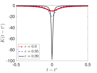
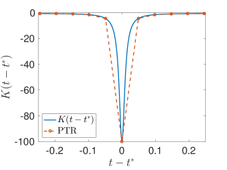
Figure 1: [Left] Plot of the kernel, $K(t-t^{\ast})$, defined in (2.5) with $a=1$ for $r=0.9$ (dot-dashed curve), $0.95$ (dashed curve), and $0.99$ (solid curve). [Right] Plot of the kernel, $K(t-t^{\ast})$, with $a=1$, and $r=0.99$ (solid curve), and the corresponding piecewise linear approximation associated with PTR₁₂₈ (dot-dashed curve).

The error, $U^{N}(r,t^{\ast})-u(r,t^{\ast})$, is not uniform in $D$. In particular, $U^{N}$ is very accurate for evaluation points far away from the boundary. On the other hand, it is $O(1)$ when $r\sim a$. The reason for this large error is due to the kernel, $K(t-t^{\ast})$. In Fig. 1, we show plots of $K$ as a function of $t-t^{\ast}$. The left plot of Fig. 1 shows that $K$ becomes sharply peaked about $t=t^{\ast}$ when $r\sim a$. We do not evaluate the double-layer potential on the boundary. Nonetheless, because $K$ becomes sharply peaked as $r\to a$, we say that the double-layer potential is nearly singular. The right plot of Fig. 1 shows that the piecewise linear approximation of $K$ used by PTR₁₂₈ will grossly overestimate the magnitude of the double-layer potential for $r=0.99a$. It is this error that leads to the $O(1)$ errors produced by PTR_N for close evaluation points. Barnett [5] has shown that this error is $O(1)$ for $a-r=O(1/N)$. In light of this result, we say that the error exhibits a boundary layer of thickness $O(1/N)$ in which it undergoes rapid growth.

In the limit as $N\to\infty$, PTR_N converges because the boundary layer vanishes at a rate of $O(1/N)$. However, that is not the limit we consider here. Rather, we study the limit as the evaluation point approaches the boundary with $N$ fixed. For that case, PTR_N is unable to accurately capture the sharp peak of the kernel about $t=t^{\ast}$ that forms as $r\to a$.

Using the error associated with PTR_N [11], we find $U^{N}$ defined in (2.6) satisfies

$$U^{N}(r,t^{\ast})=u(r,t^{\ast})+\sum_{\begin{subarray}{c}l=-\infty\\ l\neq 0\end{subarray}}^{\infty}\hat{p}[lN],$$ (2.7)

where

$$\hat{p}[k]=\frac{1}{2\pi}\int_{0}^{2\pi}K(t-t^{\ast})\mu(t)e^{-\mathrm{i}kt}\mathrm{d}t.$$ (2.8)

The error in (2.7) is aliasing of high frequencies. To determine $\hat{p}[k]$ explicitly, we use the Fourier series representation of the kernel,

$$K(t-t^{\ast})=\frac{ar\cos(t-t^{\ast})-a^{2}}{a^{2}+r^{2}-2ar\cos(t-t^{\ast})}=-\frac{1}{2}-\frac{1}{2}\sum_{m=-\infty}^{\infty}\left(\frac{r}{a}\right)^{|m|}e^{\mathrm{i}m(t-t^{\ast})},$$ (2.9)

and of the density

$$\mu(t)=\sum_{n=-\infty}^{\infty}\hat{\mu}[n]e^{\mathrm{i}nt},$$ (2.10)

to find

$$K(t-t^{\ast})\mu(t)=-\frac{1}{2}\sum_{n=-\infty}^{\infty}\hat{{\mu}}[n]e^{\mathrm{i}nt}-\frac{1}{2}\sum_{m=-\infty}^{\infty}\left(\frac{r}{a}\right)^{|m|}e^{-\mathrm{i}mt^{\ast}}\sum_{n=-\infty}^{\infty}\hat{\mu}[n]e^{\mathrm{i}(m+n)t}.$$ (2.11)

Substituting (2.11) into (2.8), and rearranging terms, we find that

$$\hat{p}[k]=-\hat{\mu}[k]-\frac{1}{2}\sum_{m=1}^{\infty}\left(\frac{r}{a}\right)^{m}\left(e^{\mathrm{i}mt^{\ast}}\hat{\mu}[k+m]+e^{-\mathrm{i}mt^{\ast}}\hat{\mu}[k-m]\right).$$ (2.12)

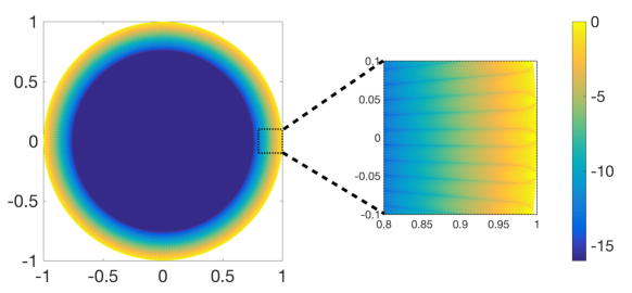
Figure 2: Contour plot of $\log_{10}|E^{N}(r,t)|$ where $E^{N}$ is given by (2.15) with $a=1$ and $N=128$.

We now obtain the error in using PTR_N to evaluate the double-layer potential by substituting (2.12) into (2.7) which yields

$$E^{N}(r,t^{\ast})=U^{N}(r,t^{\ast})-u(r,t^{\ast})=\sum_{l=1}^{\infty}\left\{-\hat{\mu}^{\ast}[lN]-\frac{1}{2}\sum_{m=1}^{\infty}\left[\left(\frac{r}{a}\right)^{m}\left(\hat{\mu}^{\ast}[lN-m]e^{\mathrm{i}mt^{\ast}}+\hat{\mu}^{\ast}[lN+m]e^{-\mathrm{i}mt^{\ast}}\right)\right]\right\}\\ +\sum_{l=1}^{\infty}\left\{-\hat{\mu}[lN]-\frac{1}{2}\sum_{m=1}^{\infty}\left[\left(\frac{r}{a}\right)^{m}\left(\hat{\mu}[lN+m]e^{\mathrm{i}mt^{\ast}}+\hat{\mu}[lN-m]e^{-\mathrm{i}mt^{\ast}}\right)\right]\right\}.$$ (2.13)

Here, we have assumed $\mu$ is real, so $\hat{\mu}[-k]=\hat{\mu}^{\ast}[k]$, where $[\cdot]^{\ast}$ denotes complex conjugation. Suppose we have chosen $N$ to be large enough so that $\hat{\mu}[lN]\ll 1$ for $l>0$. For that case, only terms in (2.13) proportional to $\hat{\mu}[lN-m]$ will substantially contribute to the error. By neglecting the other terms, we obtain

$$E^{N}(r,t^{\ast})\sim-\sum_{l=1}^{\infty}\sum_{m=1}^{\infty}\left(\frac{r}{a}\right)^{m}\left[\text{Re}\{\hat{\mu}[lN-m]\}\cos(mt^{\ast})+\text{Im}\{\hat{\mu}[lN-m]\}\sin(mt^{\ast})\right].$$ (2.14)

Equation (2.14) is the asymptotic error made by PTR_N. The key point is that when $N$ is fixed, this error is not uniform for $r\in[0,a)$. When $r\ll a$, we see that the error is much smaller than when $r\sim a$. Consider the specific case in which $\mu=1$, so that $\hat{\mu}[0]=1$ and $\hat{\mu}[k]=0$ for all $k\neq 0$. For that case, (2.14) simplifies to

$$E^{N}(r,t^{\ast})\sim\frac{\left(\frac{r}{a}\right)^{2N}-\left(\frac{r}{a}\right)^{N}\cos(Nt^{\ast})}{1+\left(\frac{r}{a}\right)^{2N}-2\left(\frac{r}{a}\right)^{N}\cos(Nt^{\ast})}.$$ (2.15)

According to (2.15), $|E^{N}(a(1-\varepsilon),t^{\ast})|=O((1-\varepsilon)^{N})=O(e^{-\varepsilon N})$, and $|E^{N}(r,t^{\ast})|\to 1/2$ as $r\to a$. These results show that $E^{N}$ has a boundary layer of thickness $O(1/N)$ where it exponentially increases to values that are $O(1)$. Fig. 2 shows a plot of (2.15) over the entire circular disk and a close-up near the boundary. These plots show the boundary layer about $r=a$ where the error attains $O(1)$ values. In practice, we would like to set $N$ based on the resolution required to solve the boundary integral equation. It is neither desirable nor practical to increase $N$ just to reduce aliasing in the evaluation of the double-layer potential. In light of this, we make the following observations.

• Equation (2.13) gives the error incurred by PTR_N to approximate the double-layer potential. This error is due to aliasing. Equation (2.14) gives the asymptotic approximation of this error when the $N$-point grid sufficiently samples $\mu$.

• The aliasing error is not uniform with respect to $r$. For the case in which $\mu=1$, the asymptotic error simplifies to (2.15). From this result, we find that the error grows rapidly and becomes $O(1)$ in a boundary layer of thickness $O(1/N)$ near the boundary. This boundary layer is shown in Fig. 2.

• For points within the boundary layer, the sharply peaked kernel causes aliasing due to insufficient resolution. Fig. 1 shows how the sharp peak of the kernel when $r/a=0.99$ is under-resolved on the grid for PTR₁₂₈.

Alternatively, by substituting (2.9) and (2.10) into (2.5), we obtain

$$u(r,t^{\ast})=\sum_{n=-\infty}^{\infty}\hat{K}^{\ast}[n]\hat{\mu}[n]e^{-\mathrm{i}nt^{\ast}}\approx\sum_{n=-N/2}^{N/2-1}\hat{K}^{\ast}[n]\hat{\mu}[n]e^{-\mathrm{i}nt^{\ast}}.$$ (2.16)

Since the coefficients, $\hat{\mu}[n]$ for $n=-N/2,\cdots,N/2-1$, can be computed readily using the Fast Fourier Transform, we introduce the truncated sum as an approximation in (2.16). The decay of $\hat{\mu}[n]$ controls the error of this approximation. Therefore, choosing $N$ to accurately solve the boundary integral equation yields a spectrally accurate approximation of the double-layer potential.

For general problems, we do not know $\hat{K}[n]$ explicitly as we do here. Instead, we compute an asymptotic expansion of the sharply peaked kernel. We determine the Fourier coefficients of this asymptotic expansion explicitly. Hence, we evaluate its contribution to the double-layer potential using an approximation like the one in (2.16). By removing the kernel’s sharp peak in this way, we are left with a smooth function to integrate using the PTR_N. We present this method to evaluate the double-layer potential for the interior Dirichlet problem for Laplace’s equation in Section 3, and the single-layer potential for the exterior Neumann problem for Laplace’s equation in Section 4.

3 Double-layer potential for the interior Dirichlet problem

Consider a simply connected, open set denoted by $D\subset\mathbb{R}^{2}$, with analytic boundary $\partial D$. Let $\overline{D}=D\cup\partial D$. The function $u\in C^{2}(D)\cap C^{1}(\overline{D})$ satisfies

$$\Delta u=0\quad\text{in $D$},$$ (3.1a)

$$u=f\quad\text{on $\partial D$},$$ (3.1b)

with $f$ an analytic function. We seek $u$ as the double-layer potential [21],

$$u(\mathbf{x})=\frac{1}{2\pi}\int_{\partial D}K(\mathbf{x},\mathbf{y})\mu(\mathbf{y})\mathrm{d}\sigma_{y},\quad\mathbf{x}\in D,$$ (3.2)

with

$$K(\mathbf{x},\mathbf{y})=\mathbf{n}_{y}\cdot\frac{\mathbf{x}-\mathbf{y}}{|\mathbf{x}-\mathbf{y}|^{2}}.$$ (3.3)

The density, $\mu$, satisfies the boundary integral equation,

$$-\frac{1}{2}\mu(\mathbf{y})+\frac{1}{2\pi}\int_{\partial D}K(\mathbf{y},\mathbf{y^{\prime}})\mu(\mathbf{y}^{\prime})\mathrm{d}\sigma_{y^{\prime}}=f(\mathbf{y}),\quad\mathbf{y}\in\partial D.$$ (3.4)

In what follows, we assume that we have solved (3.4) using PTR_N.

Figure 3: Sketch of the quantities introduced in (3.5) to study evaluation points close to the boundary.

To evaluate (3.2) when $\mathbf{x}$ is close to the boundary, we set

$$\mathbf{x}=\mathbf{y}^{\ast}-\frac{\varepsilon}{|\kappa^{\ast}|}\mathbf{n}_{y}^{\ast},$$ (3.5)

where $\mathbf{y}^{\ast}$ is the closest point to $\mathbf{x}$ on the boundary, $\mathbf{n}_{y}^{\ast}$ is the unit, outward normal at $\mathbf{y}^{\ast}$, $\kappa^{\ast}$ is the signed curvature at $\mathbf{y}^{\ast}$, and $\varepsilon>0$ is a small parameter. Fig. 3 gives a sketch of these quantities. Substituting (3.5) into (3.3) yields

$$K\left(\mathbf{y}^{\ast}-\frac{\varepsilon}{|\kappa^{\ast}|}\mathbf{n}_{y}^{\ast},\mathbf{y}\right)=\frac{|\kappa^{\ast}|}{\varepsilon}\frac{\mathbf{n}_{y}\cdot|\kappa^{\ast}|(\mathbf{y}^{\ast}-\mathbf{y})/\varepsilon-\mathbf{n}_{y}\cdot\mathbf{n}_{y}^{\ast}}{|\kappa^{\ast}(\mathbf{y}^{\ast}-\mathbf{y})/\varepsilon|^{2}-2\mathbf{n}_{y}^{\ast}\cdot|\kappa^{\ast}|(\mathbf{y}^{\ast}-\mathbf{y})/\varepsilon+1}.$$ (3.6)

We have written $K$ in (3.6) to reveal its inherent dependence on the stretched variable, $\mathbf{y}=\mathbf{y}^{\ast}+\varepsilon\mathbf{Y}/|\kappa^{\ast}|$.

3.1 Matched asymptotic expansion of the kernel

We determine the matched asymptotic expansion of (3.6) [9]. Consider first the outer expansion in which $\mathbf{y}^{\ast}$ and $\mathbf{y}$ are held fixed and $\varepsilon\to 0^{+}$, so that $|\mathbf{Y}|\to\infty$. To leading order, we find that

$$K^{\text{out}}\sim-\frac{|\kappa^{\ast}|}{\varepsilon}\frac{\mathbf{n}_{y}\cdot\mathbf{Y}}{|\mathbf{Y}|^{2}}=\frac{\mathbf{n}_{y}\cdot(\mathbf{y}^{\ast}-\mathbf{y})}{|\mathbf{y}^{\ast}-\mathbf{y}|^{2}}.$$ (3.7)

The error of (3.7) is $O(\varepsilon)$. Since this outer expansion is the kernel in (3.4), we find that

$$\frac{1}{2\pi}\int_{\partial D}K^{\text{out}}(\mathbf{y}^{\ast}-\mathbf{y})\mu(\mathbf{y})\mathrm{d}\sigma_{y}=f(\mathbf{y}^{\ast})+\frac{1}{2}\mu(\mathbf{y}^{\ast}).$$ (3.8)

The inner expansion is (3.6) written in terms of the stretched variable, $\mathbf{Y}$. We seek an explicit parameterization of this inner expansion using $\mathbf{y}(t)=(y_{1}(t),y_{2}(t))$, with $t\in[0,2\pi]$. It follows that $\mathrm{d}\sigma_{y}=|\mathbf{y}^{\prime}(t)|\mathrm{d}t$, the unit tangent is $\boldsymbol{\tau}_{y}(t)=(y_{1}^{\prime}(t),y_{2}^{\prime}(t))/|\mathbf{y}^{\prime}(t)|$, the outward unit normal is $\mathbf{n}_{y}(t)=(y_{2}^{\prime}(t),-y_{1}^{\prime}(t))/|\mathbf{y}^{\prime}(t)|$, and the signed curvature is $\kappa(t)=(y_{1}^{\prime}(t)y_{2}^{\prime\prime}(t)-y_{1}^{\prime\prime}(t)y_{2}^{\prime}(t))/|\mathbf{y}^{\prime}({t})|^{3}$. Let $\mathbf{y}^{\ast}=\mathbf{y}(t^{\ast})$ and $\kappa^{\ast}=\kappa(t^{\ast})$ with $t^{\ast}\in[0,2\pi]$. We introduce the stretched parameter, $t=t^{\ast}+\varepsilon T$, and find by expanding about $\varepsilon=0$ that

$$\mathbf{y}(t^{\ast}+\varepsilon T)=\mathbf{y}(t^{\ast})+\varepsilon T|\mathbf{y}^{\prime}(t^{\ast})|\boldsymbol{\tau}_{y}(t^{\ast})-\frac{1}{2}\varepsilon^{2}T^{2}\left[\kappa^{\ast}|\mathbf{y}^{\prime}(t^{\ast})|^{2}\mathbf{n}_{y}(t^{\ast})-(\boldsymbol{\tau}_{y}(t^{\ast})\cdot\mathbf{y}^{\prime\prime}(t^{\ast}))\boldsymbol{\tau}_{y}(t^{\ast})\right]+O(\varepsilon^{3}).$$ (3.9)

It follows that

$$\mathbf{n}_{y}(t^{\ast}+\varepsilon T)\cdot|\kappa^{\ast}|(\mathbf{y}(t^{\ast})-\mathbf{y}(t^{\ast}+\varepsilon T))=-\frac{1}{2}\varepsilon^{2}T^{2}\gamma^{\ast}+O(\varepsilon^{3}),$$ (3.10)

$$\mathbf{n}_{y}(t^{\ast})\cdot|\kappa^{\ast}|(\mathbf{y}(t^{\ast})-\mathbf{y}(t^{\ast}+\varepsilon T))=\frac{1}{2}\varepsilon^{2}T^{2}\gamma^{\ast}+O(\varepsilon^{3}),$$ (3.11)

$$\mathbf{n}_{y}(t^{\ast}+\varepsilon T)\cdot\mathbf{n}_{y}(t^{\ast})=1-\frac{1}{2}\varepsilon^{2}T^{2}|\gamma^{\ast}|^{2}+O(\varepsilon^{3}),$$ (3.12)

and

$$|\kappa(t^{\ast})[\mathbf{y}(t^{\ast})-\mathbf{y}(t^{\ast}+\varepsilon T)]|^{2}=\varepsilon^{2}T^{2}|\gamma^{\ast}|+O(\varepsilon^{3}),$$ (3.13)

with $\gamma^{\ast}=\text{sgn}[\kappa^{\ast}]|\kappa^{\ast}\mathbf{y}^{\prime}(t^{\ast})|^{2}$. Here, $\text{sgn}[x]=x/|x|$ for $x\neq 0$ and $\text{sgn}[x]=0$ for $x=0$. Substituting (3.10) – (3.13) into (3.6), we find that

$$K^{\text{in}}(T;\varepsilon)=|\kappa(t^{\ast})|\frac{-\varepsilon-\frac{1}{2}\varepsilon^{2}T^{2}\gamma^{\ast}+O(\varepsilon^{3})}{\varepsilon^{2}T^{2}|\gamma^{\ast}|+\varepsilon^{2}+O(\varepsilon^{3})}.$$ (3.14)

Next, we substitute $\varepsilon^{2}T^{2}\sim 2-2\cos(t-t^{\ast})$ into (3.14) and determine that the leading order asymptotic behavior of $K^{\text{in}}$ is given by

$$K^{\text{in}}(t-t^{\ast};\varepsilon)\sim|\kappa(t^{\ast})|\frac{-(\gamma^{\ast}+\varepsilon)+\gamma^{\ast}\cos(t-t^{\ast})}{(2|\gamma^{\ast}|+\varepsilon^{2})-2|\gamma^{\ast}|\cos(t-t^{\ast})}.$$ (3.15)

The error of (3.15) is at most $O(\varepsilon)$.

To form the leading order matched asymptotic expansion, we establish asymptotic matching in the overlap region of the outer and inner expansions. We first evaluate (3.7) in the limit as $\mathbf{y}\to\mathbf{y}^{\ast}$ and find that

$$K^{\text{out}}\to-\frac{\kappa^{\ast}}{2},\quad\mathbf{y}\to\mathbf{y}^{\ast}.$$ (3.16)

Next, we evaluate (3.15) in the limit as $\varepsilon\to 0^{+}$ and find that

$$K^{\text{in}}\to-\frac{\kappa^{\ast}}{2},\quad\varepsilon\to 0^{+}.$$ (3.17)

Thus, the overlapping value is $-\kappa^{\ast}/2$. It follows that the matched asymptotic expansion for the kernel of the double-layer potential is given by

$$K=K^{\text{out}}+K^{\text{in}}+\frac{\kappa^{\ast}}{2}+O(\varepsilon),\quad\varepsilon\to 0^{+},$$ (3.18)

with $K^{\text{out}}$ given in (3.7) and $K^{\text{in}}$ given in (3.15). The error of this matched asymptotic expansion has $O(\varepsilon)$ error because the error of $K^{\text{out}}$ given by (3.7) is $O(\varepsilon)$, and $K^{\text{in}}$ given by (3.15) is at most $O(\varepsilon)$. For example, we plot $K$, $K^{\text{in}}$, and $K^{\text{out}}$ in Fig. 4 as a function of $t-t^{\ast}$ with $t^{\ast}=\pi$ and $\varepsilon=0.1$ for the boundary curve $r(t)=1+0.3\cos 5t$. The right plot shows the $L_{\infty}$-error made by (3.18) as a function of $\varepsilon$. The solid curve is the linear fit through these data and has slope $1.2034$ consistent with the $O(\varepsilon)$ error.

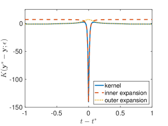
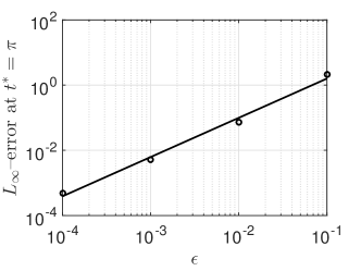
Figure 4: [Left] Plot of the kernel, $K$, given in (3.6) (solid curve) and the leading order behavior of its inner expansion, $K^{\text{in}}$ given in (3.15) (dashed curve) and its outer expansion, $K^{\text{out}}$ given in (3.7) (dotted curve) as a function of $t-t^{\ast}$ with $t^{\ast}=\pi$ and $\varepsilon=0.1$ for the boundary curve, $r(t)=1+0.3\cos 5t$. [Right] $L_{\infty}$–error of the matched asymptotic expansion given in (3.18) evaluated at $t^{\ast}=\pi$ for $\varepsilon=0.0001$, $0.001$, $0.01$, and $0.1$. These computed errors are plotted as circles. The solid curve gives the result of fitting this data to the function, $C\varepsilon^{p}$. This fit produced $p=1.2034$ indicating the $O(\varepsilon)$ error of the matched asymptotic expansion.

3.2 Fourier coefficients of $K^{\text{in}}$

The inner expansion given by (3.15) accurately captures the sharp peak of the kernel at $t=t^{\ast}$ in the limit as $\varepsilon\to 0^{+}$ as shown in Fig. 4. To avoid using PTR_N to integrate over this sharp peak, we seek the Fourier coefficients,

$$\hat{K}^{\text{in}}[n]=\frac{1}{2\pi}\int_{0}^{2\pi}K^{\text{in}}(t;\varepsilon)e^{-\mathrm{i}nt}\mathrm{d}t,$$ (3.19)

so that we may use an approximation similar to that given in (2.16). To do so, we rewrite (3.15) as

$$K^{\text{in}}(t-t^{\ast};\varepsilon)=-\frac{|\kappa(t^{\ast})|}{C_{0}}\frac{\frac{1}{2}A_{0}-A_{1}\cos(t-t^{\ast})}{1+C_{1}\cos(t-t^{\ast})},$$ (3.20)

with $A_{0}=2(\gamma^{\ast}+\varepsilon),$ $A_{1}=\gamma^{\ast},$ $C_{0}=2|\gamma^{\ast}|+\varepsilon^{2},$ and $C_{1}=-2|\gamma^{\ast}|/C_{0}.$ Equation (3.20) gives $K^{\text{in}}$ as a rational function of trigonometric polynomials which have been studied by Geer [15] in the context of constructing Fourier-Padé approximations. Since $|C_{1}|<1$, we have

$$\hat{K}^{\text{in}}[n]=\begin{cases}\frac{1+\rho^{2}}{1-\rho^{2}}\left(\frac{A_{0}}{2}+A_{1}\rho\right),&n=0\\ \frac{1+\rho^{2}}{1-\rho^{2}}\left(\frac{A_{0}\rho^{|n|}}{4}+A_{1}(\rho^{|n|-1}+\rho^{|n|+1})\right),&n\neq 0\end{cases},$$ (3.21)

where $\rho=\left(\sqrt{1-C_{1}^{2}}-1\right)/C_{1}$.

We find that we can improve on our approximation by considering the specific case in which the boundary is a circle of radius $a$. For that case, $K^{\text{out}}=-\kappa^{\ast}/2$ which cancels with the asymptotic matching term in (3.18). If we set

$$A_{0} =2(\gamma^{\ast}+\varepsilon-\varepsilon|\gamma^{\ast}|),$$ (3.22a)

$$A_{1} =\gamma^{\ast}-\varepsilon|\gamma^{\ast}|,$$ (3.22b)

$$C_{0} =2(|\gamma^{\ast}|-\varepsilon\gamma^{\ast})+\varepsilon^{2},$$ (3.22c)

$$C_{1} =-2(|\gamma^{\ast}|-\varepsilon\gamma^{\ast})/C_{0},$$ (3.22d)

instead of the coefficients defined above, we find that (3.20) gives the exact evaluation of the kernel at $r=a(1-\varepsilon)$. For this reason, we use (3.22) in (3.20) and (3.21) in practice. These coefficients just include the $O(\varepsilon^{3}T^{2})$ terms in the asymptotic expansion of $K^{\text{in}}$ for a general boundary.

To compute the contribution by $K^{\text{in}}$ to the double-layer potential, we use the approximation

$$\frac{1}{2\pi}\int_{0}^{2\pi}K^{\text{in}}(t-t^{\ast};\varepsilon)\mu(t)|\mathbf{y}^{\prime}(t)|\mathrm{d}t\approx\sum_{n=-N/2}^{N/2-1}\hat{K}^{\text{in}\ast}[n]\hat{\mu}_{y}[n]e^{-\mathrm{i}nt^{\ast}},$$ (3.23)

with

$$\hat{\mu}_{y}[n]=\frac{1}{2\pi}\int_{0}^{2\pi}\mu(t)|\mathbf{y}^{\prime}(t)|e^{-\mathrm{i}nt}\mathrm{d}t.$$ (3.24)

We use (3.21) and compute (3.24) using the Fast Fourier Transform to evaluate the approximation in (3.23). Provided that $N$ is chosen to solve boundary integral equation (3.4) so that $\mu(t)|\mathbf{y}^{\prime}(t)|$ is sufficiently resolved, the approximation in (3.23) is spectrally accurate.

3.3 Evaluating the double-layer potential

The new method developed here for close evaluation of the double-layer potential uses (3.18). For convenience, let us introduce the residual kernel,

$$\tilde{K}=K-K^{\text{out}}-K^{\text{in}}-\frac{\kappa^{\ast}}{2}.$$ (3.25)

$\tilde{K}=O(\varepsilon)$ and more importantly, it does not have a sharp peak about $t=t^{\ast}$. We rewrite the double-layer potential as

$$u\left(\mathbf{y}^{\ast}-\frac{\varepsilon}{|\kappa^{\ast}|}\mathbf{n}_{y}^{\ast}\right)=\frac{1}{2\pi}\int_{0}^{2\pi}\tilde{K}(t-t^{\ast};\varepsilon)\mu(t)|\mathbf{y}^{\prime}(t)|\mathrm{d}t+\frac{1}{2\pi}\int_{0}^{2\pi}K^{\text{out}}(t-t^{\ast};\varepsilon)\mu(t)|\mathbf{y}^{\prime}(t)|\mathrm{d}t\\ +\frac{1}{2\pi}\int_{0}^{2\pi}K^{\text{in}}(t-t^{\ast};\varepsilon)\mu(t)|\mathbf{y}^{\prime}(t)|\mathrm{d}t+\frac{\kappa^{\ast}}{4\pi}\int_{0}^{2\pi}\mu(t)|\mathbf{y}^{\prime}(t)|\mathrm{d}t.$$ (3.26)

Substituting (3.8) and (3.23) into (3.26), we obtain

$$u\left(\mathbf{y}^{\ast}-\frac{\varepsilon}{|\kappa^{\ast}|}\mathbf{n}_{y}^{\ast}\right)\approx\frac{1}{2\pi}\int_{0}^{2\pi}\left[\tilde{K}(t-t^{\ast};\varepsilon)+\frac{\kappa^{\ast}}{2}\right]\mu(t)|\mathbf{y}^{\prime}(t)|\mathrm{d}t+f(\mathbf{y}(t^{\ast}))+\frac{1}{2}\mu(t^{\ast})+\sum_{n=-N/2}^{N/2-1}\hat{K}^{\text{in}\ast}[n]\hat{\mu}_{y}[n]e^{-\mathrm{i}nt^{\ast}}.$$ (3.27)

Applying PTR_N with $t_{j}=2\pi j/N$ to the remaining integral in (3.27), we arrive at

$$u\left(\mathbf{y}^{\ast}-\frac{\varepsilon}{|\kappa^{\ast}|}\mathbf{n}_{y}^{\ast}\right)\approx\frac{1}{N}\sum_{j=1}^{N}\left[\tilde{K}(t_{j}-t^{\ast};\varepsilon)+\frac{\kappa^{\ast}}{2}\right]\mu(t_{j})|\mathbf{y}^{\prime}(t_{j})|+f(\mathbf{y}(t^{\ast}))+\frac{1}{2}\mu(t^{\ast})+\sum_{n=-N/2}^{N/2-1}\hat{K}^{\text{in}\ast}[n]\hat{\mu}_{y}[n]e^{-\mathrm{i}nt^{\ast}}.$$ (3.28)

Equation (3.28) gives our method for computing the double-layer potential for close evaluation points. It avoids aliasing incurred by the sharp peak of $K^{\text{in}}$ by using (3.23). Integration of $K^{\text{out}}$ is replaced by $f(\mathbf{y}^{\ast})+\frac{1}{2}\mu(\mathbf{y}^{\ast})$, which comes from evaluating boundary integral equation (3.4) at $\mathbf{y}^{\ast}$. PTR_N is now used only to integrate the term with the kernel, $\tilde{K}+\kappa^{\ast}/2$. This term is important for taking into account additional, non-local contributions to the double-layer potential, which may be significant.

3.4 Numerical results

We present results of this method for evaluating the double-layer potential by computing the harmonic function, $u(\mathbf{x})=-\frac{1}{2\pi}\log|\mathbf{x}-\mathbf{x}_{0}|$ with $\mathbf{x}_{0}={(1.85,1.65)}$. We compute the solution interior to the boundary curve, $r(t)=1.55+0.4\cos 5t$. The Dirichlet data in (3.1b) is determined by evaluating the harmonic function on the boundary. Boundary integral equation (3.4) is solved using PTR_N and we use the resulting density, $\mu(t_{j})$ with $t_{j}=2\pi j/N$ for $j=1,\cdots,N$ in the double-layer potential. We evaluate the double-layer potential using two methods: (1) PTR_N and (2) asymptotic PTR_N, the new method given in (3.28). We present the solution on a body-fitted grid in which evaluation points are found by moving along the normal into the domain from boundary grid points. The solution is evaluated on a grid of $200$ equispaced points along each normal starting at the boundary until we reach a distance $1/\kappa_{\max}$ from the boundary, where $\kappa_{\max}=\max_{0\leq t^{\ast}<2\pi}|\kappa(t^{\ast})|$. This grid captures the boundary layer, but does not coincide exactly with it since the boundary layer depends on the local curvature. For regions of high curvature, this body-fitted grid extends beyond the boundary layer.

In Fig. 5 we show the errors ($\log_{10}$-scale) in computing the double-layer potential using PTR₁₂₈ and asymptotic PTR₁₂₈. These results show that asymptotic PTR_N produces errors that are several orders of magnitude smaller than those of the PTR_N. To give an indication of this improvement, the $L_{\infty}$ error is $8.03$ for PTR₁₂₈ and $1.85\times 10^{-4}$ for asymptotic PTR₁₂₈. To examine this error in more detail, we show in Fig. 6 a plot of the error in computing the double-layer potential evaluated at the points indicated in Fig. 5 ($t^{\ast}=0$, $t^{\ast}=\pi/2$, and $t^{\ast}=\pi$) as a function of $\varepsilon$. These three cases are plotted over different ranges of $\varepsilon$ corresponding to $0<\varepsilon<\kappa(t^{\ast})/\kappa_{\max}$. We observe that asymptotic PTR_N does significantly better than PTR_N for small $\varepsilon$ as expected. It reduces the $O(1)$ error by at least four orders of magnitude. We find similar results over all values of $t^{\ast}$.

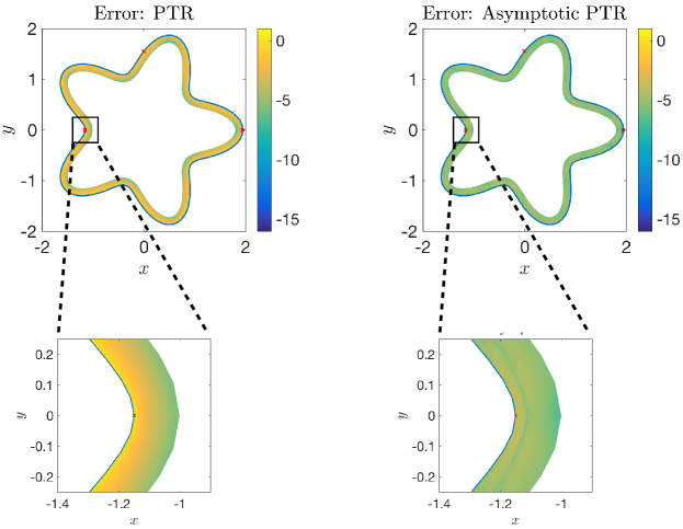
Figure 5: [Left] Plot of absolute error ($\log_{10}$-scale) in computing the double-layer potential using PTR₁₂₈ for the boundary $r(t)={1.55+0.4\cos 5t}$ for the Dirichlet data, $f(\mathbf{y})=\frac{1}{2\pi}\log|\mathbf{y}-\mathbf{x}_{0}|$ with $\mathbf{x}_{0}={(1.85,1.65)}$. [Right] Plot of absolute error ($\log_{10}$-scale) in computing the double-layer potential using the asymptotic PTR₁₂₈ given in (3.28) for the same problem. The “$\times$” symbols on the boundary indicates the points corresponding to $t^{\ast}=0$, $t^{\ast}=\pi/2$, and $t^{\ast}=\pi$.

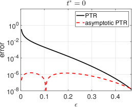
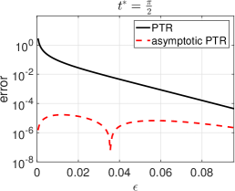
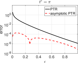
Figure 6: Plot of the absolute error as a function of $\varepsilon$ made in evaluating the double-layer potential for different $t^{\ast}$ values using PTR₁₂₈ (solid curve) and using asymptotic PTR₁₂₈ (dashed curve).

We can further improve the new method using the identity for the double-layer potential [21] (see (5.1)) to rewrite (3.2) as follows:

$$u(\mathbf{x})=\frac{1}{2\pi}\int_{\partial D}K(\mathbf{x},\mathbf{y})(\mu(\mathbf{y})-\mu(\mathbf{y}^{\ast}))\mathrm{d}\sigma_{y}-\mu(\mathbf{y}^{\ast}),\quad\mathbf{x}\in\partial D.$$ (3.29)

In (3.29), the integrand is now smoother as it vanishes at the point $\mathbf{y}=\mathbf{y}^{\ast}$, and the error using PTR_N drastically decreases. Applying asymptotic PTR_N to (3.29), we obtain

$$u\left(\mathbf{y}^{\ast}-\frac{\varepsilon}{|\kappa^{\ast}|}\mathbf{n}_{y}^{\ast}\right)\approx\frac{1}{N}\sum_{j=1}^{N}\left[\tilde{K}(t_{j}-t^{\ast};\varepsilon)+\frac{\kappa^{\ast}}{2}\right](\mu(t_{j})-\mu(t^{\ast}))|\mathbf{y}^{\prime}(t_{j})|+f(\mathbf{y}(t^{\ast}))+\sum_{n=-N/2}^{N/2-1}\hat{K}^{\text{in}\ast}[n]\hat{\mu}^{\ast}_{y}[n]e^{-\mathrm{i}nt^{\ast}}$$ (3.30)

with

$$\hat{\mu}^{\ast}_{y}[n]=\frac{1}{2\pi}\int_{0}^{2\pi}(\mu(t)-\mu(t^{\ast}))|\mathbf{y}^{\prime}(t)|e^{-\mathrm{i}nt}\mathrm{d}t.$$ (3.31)

For the example problem discussed above, the $L_{\infty}$ error is $7.13\times 10^{-5}$ for PTR₁₂₈ applied to (3.29), and $2.54\times 10^{-5}$ for asymptotic PTR₁₂₈ given by (3.30). This additional improvement (3.29) is only valid for the double-layer potential and does not generalize.

4 Single-layer potential for the exterior Neumann problem

We now consider the exterior Neumann problem,

$$\Delta v=0\quad\text{in $\mathbb{R}^{2}\backslash\bar{D}$},$$ (4.1a)

$$\frac{\partial v}{\partial n}=g\quad\text{on $\partial D$},$$ (4.1b)

with $g$ denoting an analytic function satisfying

$$\int_{\partial D}g(\mathbf{y})\mathrm{d}\sigma_{y}=0.$$ (4.2)

We seek $v$ as the single-layer potential [21],

$$v(\mathbf{x})=\frac{1}{2\pi}\int_{\partial D}S(\mathbf{x},\mathbf{y})\varphi(\mathbf{y})\mathrm{d}\sigma_{y},\quad\mathbf{x}\in\mathbb{R}^{2}\backslash\bar{D},$$ (4.3)

with

$$S(\mathbf{x},\mathbf{y})=-\log|\mathbf{x}-\mathbf{y}|.$$ (4.4)

The density, $\varphi(\mathbf{y})$, satisfies the boundary integral equation,

$$-\frac{1}{2}\varphi(\mathbf{y})+\frac{1}{2\pi}\int_{\partial D}\frac{\partial S(\mathbf{y},\mathbf{y^{\prime}})}{\partial n_{y}}\varphi(\mathbf{y}^{\prime})\mathrm{d}\sigma_{y^{\prime}}=g(\mathbf{y}),\quad\mathbf{y}\in\partial D.$$ (4.5)

To study the close evaluation of (4.3), we now set

$$\mathbf{x}=\mathbf{y}^{\ast}+\frac{\varepsilon}{|\kappa^{\ast}|}\mathbf{n}_{y}^{\ast}.$$ (4.6)

Substituting (4.6) into (4.4), we obtain

$$S\left(\mathbf{y}^{\ast}+\frac{\varepsilon}{|\kappa^{\ast}|}\mathbf{n}_{y}^{\ast},\mathbf{y}\right)=-\log\varepsilon+\log|\kappa^{\ast}|-\frac{1}{2}\log\left(|\kappa^{\ast}(\mathbf{y}^{\ast}-\mathbf{y})/\varepsilon|^{2}+2\mathbf{n}_{y}^{\ast}\cdot|\kappa^{\ast}|(\mathbf{y}^{\ast}-\mathbf{y})/\varepsilon+1\right).$$ (4.7)

Just as we have done for $K$ in (3.6), we have written (4.7) to show the underlying dependence on the stretched variable, $\mathbf{y}=\mathbf{y}^{\ast}+\varepsilon\mathbf{Y}/|\kappa^{\ast}|$.

The outer expansion of (4.7) is $S^{\text{out}}\sim-\log|\mathbf{y^{\ast}}-\mathbf{y}|$. This outer expansion is singular. In contrast to the double-layer potential, this outer expansion does not correspond to the kernel boundary integral equation (4.5). One could use a high order quadrature rule that explicitly takes into account this singularity [3, 20]. However, we choose to not use one here because we find in the numerical examples below that our method significantly reduces the dominant error. To compute the inner expansion, $S^{\text{in}}$, we introduce the stretched parameter, $t=t^{\ast}+\varepsilon T$ into the same parameterization of the boundary used for the double-layer potential. Making use of (3.10) and (3.12), we find by expanding as $\varepsilon\to 0^{+}$ that

$$S^{\text{in}}(T;\varepsilon)=\log|\kappa^{\ast}|-\frac{1}{2}\log\left(\varepsilon^{2}T^{2}|\gamma^{\ast}|+\varepsilon^{2}+O(\varepsilon^{3})\right).$$ (4.8)

Substituting $\varepsilon^{2}T^{2}\sim 2-2\cos(t-t^{\ast})$, we find that to leading order,

$$S^{\text{in}}(t-t^{\ast};\varepsilon)\sim\log|\kappa^{\ast}|-\frac{1}{2}\log\left((2|\gamma^{\ast}|+\varepsilon^{2})-2|\gamma^{\ast}|\cos(t-t^{\ast})\right).$$ (4.9)

4.1 Fourier coefficients of $S^{\text{in}}$

Using the modified coefficients introduced in (3.22), we write (4.9) as

$$S^{\text{in}}(t-t^{\ast};\varepsilon)\sim\log|\kappa^{\ast}|-\frac{1}{2}\log C_{0}-\frac{1}{2}\log[1+C_{1}\cos(t-t^{\ast})].$$ (4.10)

We now seek to compute

$$\hat{S}^{\text{in}}[n]=\delta_{n,0}\left[\log|\kappa^{\ast}|-\frac{1}{2}\log C_{0}\right]-\frac{1}{2\pi}\int_{0}^{2\pi}\frac{1}{2}\log[1+C_{1}\cos(t-t^{\ast})]e^{-\mathrm{i}nt}\mathrm{d}t,$$ (4.11)

with $\delta_{n,0}$ denoting the Kronecker delta. To compute the integral in (4.11), we start with

$$\frac{\mathrm{d}}{\mathrm{d}t}\log[1+C_{1}\cos(t-t^{\ast})]=\frac{C_{1}\sin(t-t^{\ast})}{1+C_{1}\cos(t-t^{\ast})}.$$ (4.12)

The right-hand side of (4.12) is another example of a rational trigonometric function studied by Geer [15]. It can be readily shown that

$$\frac{1}{2\pi}\int_{0}^{2\pi}\frac{\sin(t-t^{\ast})}{1+C_{1}\cos(t-t^{\ast})}e^{\mathrm{i}nt}\mathrm{d}t=\text{sgn}(n)\frac{\mathrm{i}}{2}\frac{1+\rho^{2}}{1-\rho^{2}}\left(\rho^{|n|-1}-\rho^{|n|+1}\right),$$ (4.13)

where $\rho=\left(\sqrt{1-C_{1}^{2}}\right)/C_{1}$. It follows from term-by-term integration of the Fourier series with these coefficients that

$$\hat{S}^{\text{in}}[n]=\begin{cases}\displaystyle\log|\kappa^{\ast}|-\frac{1}{2}\log C_{0}-\frac{C_{1}}{2}\frac{1+\rho^{2}}{1-\rho^{2}}\left(\frac{1}{\rho}-\rho\right)\log(1-\rho)&n=0,\\ \displaystyle\frac{C_{1}}{4|n|}\frac{1+\rho^{2}}{1-\rho^{2}}\left(\rho^{|n|-1}-\rho^{|n|+1}\right)&n\neq 0.\end{cases}$$ (4.14)

4.2 Evaluating the single-layer potential

Given the inner expansion computed above, our method for evaluating the single-layer potential is to compute an approximation of

$$v\left(\mathbf{y}^{\ast}+\frac{\varepsilon}{|\kappa^{\ast}|}\mathbf{n}_{y}^{\ast}\right)=\frac{1}{2\pi}\int_{0}^{2\pi}\tilde{S}(t-t^{\ast})\varphi(t)|\mathbf{y}^{\prime}(t)|\mathrm{d}t+\frac{1}{2\pi}\int_{0}^{2\pi}S^{\text{in}}(t-t^{\ast};\varepsilon)\varphi(t)|\mathrm{y}^{\prime}(t)|\mathrm{d}t,$$ (4.15)

with $\tilde{S}=S-S^{\text{in}}$. We use PTR_N to evaluate the first integral with kernel, $\tilde{S}$, and a truncated convolution sum to evaluate the second integral with kernel, $S^{\text{in}}$,

$$v\left(\mathbf{y}^{\ast}+\frac{\varepsilon}{|\kappa^{\ast}|}\mathbf{n}_{y}^{\ast}\right)\approx\frac{1}{N}\sum_{j=1}^{N}\tilde{S}(t_{j}-t^{\ast})\varphi(t_{j})|\mathbf{y}^{\prime}(t_{j})|+\sum_{n=-N/2}^{N/2-1}\hat{S}^{\text{in}}[n]\hat{\varphi}_{y}[n]e^{-\mathrm{i}nt^{\ast}},$$ (4.16)

where we compute

$$\hat{\varphi}_{y}[n]=\frac{1}{2\pi}\int_{0}^{2\pi}\varphi(t)|\mathbf{y}^{\prime}(t)|e^{-\mathrm{i}nt}\mathrm{d}t,$$ (4.17)

using the Fast Fourier Transform. Just as with the double-layer potential, provided that $N$ is chosen so that it solves boundary integral equation (4.5) with sufficient accuracy, the truncated convolution sum in (4.16) is spectrally accurate.

4.3 Numerical examples

We present results for the evaluation of the single-layer potential by computing the harmonic function, $v(\mathbf{x})=(\mathbf{x}-\mathbf{x}_{0})/|\mathbf{x}-\mathbf{x}_{0}|^{2}$, with $\mathbf{x}_{0}=(0.1,0.4)$. We compute the solution exterior to the the boundary curve, $r(t)=1.55+0.4\cos 5t$. The Neumann data in (4.1b) is determined by computing the normal derivative of the harmonic function on the boundary. Boundary integral equation (4.5) is solved using PTR_N and we use the resulting density $\varphi(t_{j})$ with $t_{j}=2\pi j/N$ for $j=1,\cdots,N$ in the single-layer potential. We evaluate the single-layer potential using two methods: (1) PTR_N and (2) asymptotic PTR_N, the new method given in (4.16). We modify the body-fitted grid described above for the evaluation of the double-layer potential to evaluate exterior points. The solution is evaluated on a grid of $200$ equispaced points along each normal starting at the boundary until we reach a distance $1/\kappa_{\max}$ from the boundary.

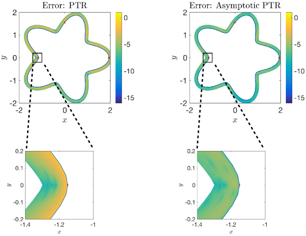
Figure 7: [Left] Plot of the absolute error ($\log_{10}$-scale) in computing the single-layer potential using PTR₁₂₈ for the boundary $r(t)={1.55+0.4\cos 5t}$ for the Neumann data, $g(\mathbf{y})=\frac{\partial v}{\partial\mathbf{n}}$ with $v(\mathbf{x})=(\mathbf{x}-\mathbf{x}_{0})/|\mathbf{x}-\mathbf{x}_{0}|^{2}$, $\mathbf{x}_{0}={(0.1,0.4)}$. [Right] Plot of the absolute error ($\log_{10}$-scale) in computing the single-layer potential using asymptotic PTR₁₂₈ given in (4.16) for the same problem. The “$\times$” symbols on the boundary indicates the points corresponding to $t^{\ast}=0$, $t^{\ast}=\pi/2$ and $t^{\ast}=\pi$.

In Fig. 7 we show the absolute error ($\log_{10}$-scale) in computing the single-layer potential using the PTR₁₂₈ and using asymptotic PTR₁₂₈. The single-layer potential kernel is not as sharply peaked as the double-layer potential kernel, so the error in evaluating the single-layer potential is less than the error when evaluating the double-layer potential. Even so, we still observe a boundary layer of thickness $O(1/N)$ in which the error is $O(1)$ due to aliasing when using PTR_N. Asymptotic PTR_N effectively reduces the error in the boundary layer. To give an indication of this improvement, the $L_{\infty}$ error is $0.113$ for PTR₁₂₈ and $5.39\times 10^{-5}$ for asymptotic PTR₁₂₈. In Fig. 8, we plot the error in computing the single-layer potential evaluated at the points indicated in Fig. 7 ($t^{\ast}=0$, $t^{\ast}=\pi/2$ and $t^{\ast}=\pi$) as a function of $\varepsilon$ with $0<\varepsilon<\kappa(t^{\ast})/\kappa_{\max}$. These plots show that the asymptotic method reduces the error by at least 3 orders of magnitude for small $\varepsilon$. We find similar results over all values of $t^{\ast}$. For the case in which $t^{\ast}=\pi$, the error of asymptotic PTR_N becomes larger than that for PTR_N for $0.36<\varepsilon<0.52$. For this particular boundary curve, $\kappa_{\max}$ is attained at $t^{\ast}=\pi$. Hence, the body-fitted grid at $t^{\ast}=\pi$ plots the single-layer potential over $0<\varepsilon<1$. For this range of $\varepsilon$, we consider points outside the boundary layer where PTR_N is competitive with, and may even become more accurate than asymptotic PTR_N. In fact, that is what is observed in Fig. 8 for $t^{\ast}=\pi$.

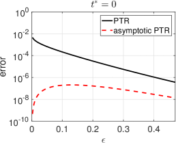
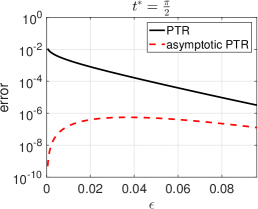
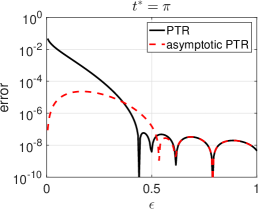
Figure 8: Plot of the absolute error as a function of $\varepsilon$ made in evaluating the single-layer potential for different $t^{\ast}$ using PTR₁₂₈ (solid curve) and using asymptotic PTR₁₂₈ (dashed curve).

5 General implementation

In the results presented above, we are using a body-fitted grid, in which evaluation points are found by moving along the normal into the domain from boundary integration points. Often the solution is needed at more generally defined points. Asymptotic PTR_N tacitly assumes in (3.5) for interior problems, or (4.6) for exterior problems, that $\mathbf{y}^{\ast}$, is the unique minimum distance from the boundary to the evaluation point, $\mathbf{x}$. In the examples, the closest point on the boundary, $\mathbf{y}^{\ast}$ coincides with a PTR_N grid point from which we extended in the normal direction. We discuss here the more general problem.

Suppose we have an evaluation point in the domain, $\mathbf{x}$. Then the first problem to address is whether $\mathbf{x}$ is, in fact, close enough to the boundary to warrant special attention and requires use of asymptotic PTR_N. To solve this problem, we make use of the identity for the double-layer potential [21],

$$\frac{1}{2\pi}\int_{\partial D}\frac{\mathbf{n}_{y}\cdot(\mathbf{x}-\mathbf{y})}{|\mathbf{x}-\mathbf{y}|^{2}}\,\mathrm{d}\sigma_{y}=\begin{cases}-1&\mathbf{x}\in D\\ -\frac{1}{2}&\mathbf{x}\in\partial D\\ \,\,\,0&\mathbf{x}\in\mathbb{R}^{2}\setminus\overline{D}\end{cases}.$$ (5.1)

Evaluating (5.1) using PTR_N suffers from the same aliasing problem that the more general layer potential evaluations do. Thus, we use it to determine if $\mathbf{x}$ lies within the boundary layer. To do this, we set a user-defined threshold for the error. If the error in evaluating (5.1) using PTR_N is less than this threshold value, we keep the result computed using PTR_N. Otherwise, we use the appropriate asymptotic approximation.

To use these asymptotic approximations, we must determine the parameter, $t^{\ast}$, where $t^{\ast}=\min_{0\leq t<2\pi}|\mathbf{x}-\mathbf{y}(t)|^{2}$. For a general boundary, this problem may not have a unique solution. In practice, we find a unique minimizer for evaluation points that are identified to be in the boundary layer using PTR_N evaluation of (5.1). Once $t^{\ast}$ is determined, all other quantities required for the asymptotic approximations follow. Finally, we evaluate the solution of the boundary value problem at hand at any point $\mathbf{x}$ using either PTR_N or asymptotic PTR_N.

We present results of this generalized method for evaluation of the double-layer potential and single-layer potential for the same problems presented in Section 3.4 and 4.3, respectively. We use a threshold of $1\times 10^{-8}$, as described above, to determine when the evaluation point is inside the boundary layer and asymptotic PTR_N method is to be used. In Fig. 9 we show the error in computing the double-layer potential using PTR₂₅₆ and asymptotic PTR₂₅₆ when solving on a Cartesian grid with meshsize $h=0.005$ within the boundary curve. Similarly, we present the evaluation of the single-layer potential in Fig. 10. Here, we are computing on a Cartesian grid with meshsize $h=0.005$ exterior to the boundary curve. These results show, similar to the results while considering a body-fitted grid, that the error made by asymptotic PTR_N is several orders of magnitude smaller than those made by PTR_N. However, there are more variations in these errors because $\mathbf{y}^{\ast}$ does not always coincide with a quadrature point. We choose to use 256 quadrature points here as this is what is actually needed to solve the boundary integral equations for the densities such that $\mu(t)|\mathbf{y}^{\prime}(t)|$ and $\varphi(t)|\mathbf{y}^{\prime}(t)|$ are sufficiently resolved. We were able to use less points for the body-fitted grid as this restriction is not as strict when $\mathbf{y}^{\ast}$ is a quadrature point.

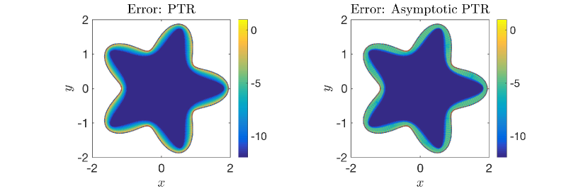
Figure 9: [Left] Plot of the absolute error ($\log_{10}$-scale) in computing the double-layer potential using PTR₂₅₆ for the boundary $r(t)={1.55+0.4\cos 5t}$ for the Dirichlet data, $f(\mathbf{y})=\frac{1}{2\pi}\log|\mathbf{y}-\mathbf{x}_{0}|$ with $\mathbf{x}_{0}={(1.85,1.65)}$. We evaluate the solution inside the domain on a regular grid. [Right] Plot of the absolute error ($\log_{10}$-scale) in computing the double-layer potential using asymptotic PTR${}_{\text{256}}$ given in (3.28) for the same problem. The asymptotic method is used in a boundary layer determined by a threshold on the error from evaluating (5.1).

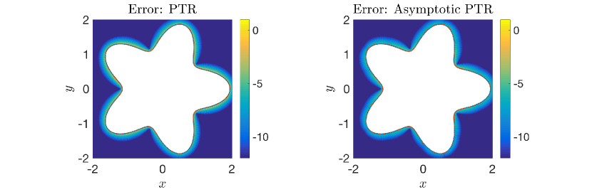
Figure 10: [Left] Plot of the absolute error ($\log_{10}$-scale) in computing the single-layer potential using PTR₂₅₆ for the boundary $r(t)={1.55+0.4\cos 5t}$ for the Neumann data, $g(\mathbf{y})=\frac{\partial v}{\partial\mathbf{n}}$ with $v(\mathbf{x})=(\mathbf{x}-\mathbf{x}_{0})/|\mathbf{x}-\mathbf{x}_{0}|^{2}$, $\mathbf{x}_{0}={(0.1,0.4)}$. [Right] Plot of $\log_{10}$ of the absolute error ($\log_{10}$-scale) in computing the single-layer potential using the asymptotic PTR₂₅₆ given in (4.16) for the same problem. The asymptotic method is used in a boundary layer determined by a threshold on the error from evaluating (5.1).

6 Conclusions

We have presented a new method to address the close evaluation problem. When solving boundary value problems using boundary integrals equation methods, the solution is evaluated at desired points within the domain by numerically evaluating layer potentials. Using the same quadrature rule that is used to solve the integral equation for this evaluation achieves high order accuracy everywhere in the domain, except close to the boundary where an $O(1)$ error is incurred. The new method developed here takes advantage of the knowledge of the sharply peaked kernel of layer potentials close to the boundary to reduce this error by several orders of magnitude. We have used asymptotic methods to analyze the kernels of the double- and single-layer potentials to relieve the numerical method from having to integrate over this sharply peaked kernel. The resulting method is straightforward to implement. We have presented results for both the interior Dirichlet problem and exterior Neumann problem for Laplace’s equation and show a reduction in error of four to five orders of magnitude in the solution evaluation close to the boundary. Furthermore, we have presented how to generalize this method to solve within the whole domain, including how to determine when to use the new asymptotic method.

This asymptotic method has been recently applied to acoustic scattering problems by sound-soft obstacles [10]. For those problems, the sharp peaks in the kernels for the single- and double-layer potentials, both which are needed, have the same character as those for Laplace’s equation discussed here. Hence, only small modifications are needed to apply these methods to wave propagation problems. We are currently extending this asymptotic method to three-dimensional problems. Furthermore, we are working on different applications which include extending the method presented here to the Stokes equations and studying surface plasmons.

References

- [1]
- [2] G. M. Akselrod, C. Argyropoulos, T. B. Hoang, C. Ciracì, C. Fang, J. Huang, D. R. Smith, M. H. Mikkelsen, Probing the mechanisms of large Purcell enhancement in plasmonic nanoantennas, Nat. Photonics 8 (2014) 835–840.
- [3] S. Avram and M. Israeli, Quadrature methods for periodic singular and weakly singular Fredholm integral equations, J. Sci. Comput. 3 (1988) 201–231.
- [4] K. Atkinson, The Numerical Solution of Integral Equations of the Second Kind, Cambridge University Press, Cambrdige, UK, 1997.
- [5] A. H. Barnett, Evaluation of layer potentials close to the boundary for Laplace and Helmholtz problems on analytic planar domains, SIAM J. Sci. Comput. 36 (2014) A427–A451.
- [6] A. Barnett, B. Wu, S. Veerapaneni, Spectrally accurate quadratures for evaluation of layer potentials close to the boundary for the 2D Stokes and Laplace equations, SIAM J. Sci. Comput. 37 (2015) B519–B542.
- [7] J. T. Beale, M.-C. Lai, A method for computing nearly singular integrals, SIAM J. Numer. Anal. 38 (2001) 1902–1925.
- [8] J. T. Beale, W. Ying, and J. Wilson, A simple method for computing singular or nearly singular integrals on closed surfaces, Comm. Comput. Phys, 20 (2016) 733–753.
- [9] C. M. Bender, S. A. Orszag, Advanced Mathematical Methods for Scientists and Engineers I: Asymptotic Methods and Perturbation Theory, Springer Science & Business Media, New York, NY, 1999.
- [10] C. Carvalho, S. Khatri, and A. D. Kim, Local analysis of near fields in acoustic scattering, 13th International Conference on Mathematical and Numerical Aspects of Wave Propagation, Minneapolis, MN, 2017.
- [11] P. J. Davis, On the numerical integration of periodic analytic functions, Proceedings of a Symposium on Numerical Approximations, ed. R. E. Langer, University of Wisconsin Press, Madison, WI, 1959.
- [12] L. M. Delves, J. Mohamed, Computational Methods for Integral Equations, Cambridge University Press, Cambridge, UK, 1988.
- [13] J. G. Fikioris and J. L. Tsalamengas, Strongly and uniformly convergent Green’s function expansions, J. Franklin Inst., 324 (1987), 1–17.
- [14] J. G. Fikioris, J. L. Tsalamengas, and G. J. Fikioris, Strongly convergent Green’s function expansions for rectangularly shielded microstrip lines, IEEE Trans. Microw. Theory Techn. and techniques 36 (1988), 1386–1396.
- [15] J. F. Geer, Rational trigonometric approximations using fourier series partial sums, J. Sci. Comput. 10 (1995) 325–356.
- [16] R. B. Guenther, J. W. Lee, Partial Differential Equations of Mathematical Physics and Integral Equations, Dover, New York, NY, 1996.
- [17] J. Helsing, R. Ojala, On the evaluation of layer potentials close to their sources, J. Comput. Phys. 227 (2008) 2899–2921.
- [18] E. E. Keaveny, M. J. Shelley, Applying a second-kind boundary integral equation for surface tractions in Stokes flow, J. Comput. Phys. 230 (2011) 2141–2159.
- [19] A. Klöckner, A. Barnett, L. Greengard, and M. O’Neil, Quadrature by expansion: A new method for the evaluation of layer potentials, J. Comput. Phys 252 (2013) 332–349.
- [20] R. Kress, Boundary integral equations in time-harmonic acoustic scattering, Mathl. Comput. Modelling 15 (1991) 228–243.
- [21] R. Kress, Linear Integral Equations, Springer-Verlag, New York, NY, 1999.
- [22] S. A. Maier, Plasmonics: Fundamentals and Applications, Springer Science & Business Media, New York, NY, 2007.
- [23] G. R. Marple, A. Barnett, A. Gillman, S. Veerapaneni, A fast algorithm for simulating multiphase flows through periodic geometries of arbitrary shape, SIAM J. Sci. Comput. 38 (2016) B740–B772.
- [24] K. M. Mayer, S. Lee, H. Liao, B. C. Rostro, A. Fuentes, P. T. Scully, C. L. Nehl, J. H. Hafner, A label-free immunoassay based upon localized surface plasmon resonance of gold nanorods, ACS Nano 2 (2008) 687–692.
- [25] L. Novotny, N. Van Hulst, Antennas for light, Nat. Photonics 5 (2011) 83–90.
- [26] T. Sannomiya, C. Hafner, J. Voros, In situ sensing of single binding events by localized surface plasmon resonance, Nano Lett. 8 (2008) 3450–3455.
- [27] D. J. Smith, A boundary element regularized Stokeslet method applied to cilia-and flagella-driven flow, Proc. R. Soc. Lond. A 465 (2009) 3605–3626.
- [28] W. A. Strauss, Partial Differential Equations, Wiley, New York, NY, 1992.