Convolutional Kitchen Sinks for Transcription Factor Binding Site Prediction

Abstract

We present a simple and efficient method for prediction of transcription factor binding sites from DNA sequence. Our method computes a random approximation of a convolutional kernel feature map from DNA sequence and then learns a linear model from the approximated feature map. Our method outperforms state-of-the-art deep learning methods on five out of six test datasets from the ENCODE consortium, while training in less than one eighth the time.

1 Introduction

Understanding binding affinity between proteins and DNA sequence is a crucial step in deciphering the regulation of gene expression. Specifically, characterizing the binding affinity of transcription factor proteins (TFs) to DNA sequence determines the relative expression of genes downstream from a TF binding site.

The recent advent of sequencing technologies, such as chromatin immunoprecipitation with massively parallel DNA sequencing (ChIP-seq), provides us with genome-wide binding specificities for 187 TFs across 98 cellular contexts of interest from the ENCODE consortium ENCODE et al., (2004). These specificities can be thresholded to define high-confidence bound and unbound regions for a given TF. Given the location of these binding sites, we can formulate a binary sequence classification problem, classifying regions bound and unbound by a TF as positive and negative, respectively. Using a binary sequence classification model, we can predict binding sites in new cellular contexts, learning regulatory behavior without the expense of ChIP-seq experiments.

String kernel methods are well understood and have been extensively used for sequence classification Jaakola et al., (1999); Eskin et al., (2002); Leslie et al., (2002). Specifically, Fletez-Brant et al. and Lee et al. Fletez-Brant et al., (2013); Lee et al., (2015) have applied string kernel methods to the prediction of transcription factor binding sites. However, kernel methods require pairwise comparison between all $n$ training sequences and thus incur an expensive $\mathcal{O}(n^{2})$ computational and storage complexity, making them computationally intractable for large data sets.

Recently, convolutional neural networks (CNN) have been successful for prediction of TF binding sites Zhou et al., (2015); Alipanahi et al., (2015); Kelley et al., (2016). CNNs generalize well by encoding spatial invariance during training. Fast convolutions on a Graphical Processing Unit (GPU) allows CNNs to train on large datasets. However, the actual design of the neural network greatly impacts model performance, yet there is no clear understanding of how to design a network for a particular task. Furthermore there is no generally accepted network architecture for the task of TF binding site prediction from DNA sequence.

In this work, we present a convolutional kernel approximation algorithm that maintains the spatial invariance and computational efficiency of CNNs. Dubbed Convolutional Kitchen Sinks (CKS), our algorithm learns a model from the output of a 1 layer random convolutional neural network Rahimi et al., (2009). All the parameters of the network are independent and identically distributed (IID) random samples from a gaussian distribution with a specified variance. We then train a linear model on the output of this network. Our results show that for five out of six transcription factors, CKS outperform current state-of-the art CNN implementations, while maintaining a simple architecture and training eight times faster than a CNN.

2 Method

The task of transcription factor (TF) binding site prediction from DNA sequence reduces to binary sequence classification. We present a randomized algorithm for finding an embedding of sequence data apt for linear classification (Algorithm 1). Our algorithm is closely related to the work of convolutional kernel networks, which approximates a convolutional kernel feature map via a nonconvex optimization objective Mairal et al., (2014). However, unlike Mairal et al. Mairal et al., (2014), we approximate the convolutional kernel feature map via random projections in the style of Rahimi et al. Rahimi et al., (2009, 2007).

We will first define the convolutional $n$-gram kernel, and then analyze why it has desired properties for the task of string classification. Note that we use the term $n$-gram to refer to a contiguous sequence of $n$ characters, whereas computational biology literature refers to the same concept as a $k$-mer.

Definition 1 (Convolutional $n$-gram kernel).

Let $x,y$ be strings of length $d$ from an underlying alphabet $\mathcal{A}$, and let $\mathds{H}(x,y)$ denote the Hamming distance between the two strings. Let $x_{i:j}$ denote the substring of $x$ from index $i$ to $j-1$. Let $n$ be an integer less than $d$ and let $\gamma$ be a real valued positive number denoting the width of the kernel. The kernel function $K_{n,\gamma}(x,y)$ is defined as:

$$K_{n,\gamma}(x,y)=\displaystyle\sum_{i=0}^{d-n}\displaystyle\sum_{j=0}^{d-n}\exp(-\gamma\mathds{H}^{2}(x_{i:i+n},y_{j:j+n}))$$ (1)

To gain intuition for the behavior of this kernel, take $\gamma$ to be a large value. It follows that $\exp(-\gamma\mathds{H}^{2}(x_{i:i+n},y_{j:j+n}))\approx\mathds{1}[x_{i:i+n}=y_{j:j+n}]$.

This combinatorial reformulation results in the following well studied Spectrum Kernel (Definition 2).

Definition 2 (Spectrum Kernel).

Let $\mathcal{S}_{n}(\mathcal{A})$ be the set of all length $n$ contiguous substrings in $\mathcal{A}$, and $\#(x,s)$ count the occurrences of $s\in x$ Leslie et al., (2002).

$$K_{spec}(x,y)=\displaystyle\sum_{s\in\mathcal{S}_{n}(\mathcal{A})}\#(x,s)\#(y,s)$$ (2)

Algorithm 1 Convolutional Kitchen Sink for sequences

0:  $x_{i}\ldots x_{N}\in\mathds{R}^{d}$ (input sequences), $\gamma$ (width of kernel), $n$ (convolution size), $M$ (the approximation dimension, number of kitchen sinks)

1:  for $j\in\left\{0\ldots M\right\}$ do

2:     $w_{j}\sim\mathcal{N}(0,\gamma I_{n})$                   Sample kitchen sink from gaussian

3:     $b_{j}\sim U(0,2\pi)$                      Sample phase from uniform disk

4:     for $i\in\left\{0\ldots N\right\}$ do

5:        $z_{ij}=w_{j}\ast x_{i}$                   Convolve filter with input sequence

6:        $c_{ij}=\cos(z_{ij}+b_{j})$             Add phase and compute element-wise cosine                                     Note $z_{ij}$ and $c_{ij}$ are vectors in $\mathcal{R}^{d-n+1}$

7:        $\phi(x_{i})_{j}=\sqrt{\frac{2}{M}}\displaystyle\sum_{k=0}^{d-n}c_{ijk}$      Average to get the $j$th output feature value for sequence $x_{i}$

8:     end for

9:  end for

9:  $\phi(x_{i})\ldots\phi(x_{N})$

Other string kernel methods such as the mismatch Eskin et al., (2002) and gapped $n$-gram kernel Ghandi et al., (2014) allow for partial mismatches between $n$-grams. We note that decreasing $\gamma$ in Equation 1 relaxes the penalty of $n$-gram mismatches between disappoints, thereby capturing the behavior of the mismatch and gapped $n$-gram kernels Eskin et al., (2002); Ghandi et al., (2014). Note that Equation 1 is computationally prohibitive, as it takes $\Omega(nd^{2})$ to compute each of the $N^{2}$ entries in the kernel matrix. Furthermore, the feature map induced by the kernel in Equation 1 is infinite dimensional, so the kernel matrix is necessary.

Instead, we turn to a random approximation of Equation 1 (see Algorithm 1). Since our kernel is a sum of non linear functions it suffices to define a feature map $\hat{\phi}$ on sequences x and y that approximates each term in the sum from Equation 1:

$$\exp(-\gamma\mathds{H}(x_{i:i+n},y_{j:j+n}))\approx\hat{\phi}(x_{i:i+n})^{T}\hat{\phi}(y_{j:j+n})$$ (3)

Claim 1 from Rahimi et al. Rahimi et al., (2007) states that for $j\in\left\{0\ldots M-1\right\}$, if we choose $\hat{\phi}(x_{i:i+n})_{j}=\sqrt{\frac{2}{M}}\cos(w_{j}^{T}x_{i:i+n}+b_{j})$, where $w_{j}\sim\mathcal{N}(0,\gamma)$, $b_{j}\sim U(0,2\pi)$, then $\hat{\phi}(x_{i:i+n})$ satisfies Equation 3. Note that to use Claim 1, we represent Hamming distance in Equation 1 as an L2 distance. We refer to each $w_{j}$ as a “random kitchen sink". The result in in Rahimi et al. Rahimi et al., (2007) (Claim 1) gives strong guarantees that $\hat{\phi}(x)^{T}\hat{\phi}(y)$ concentrates exponentially fast to Equation 1, which means we can set $M$, the number of kitchen sinks, to be small.

Algorithm 1 details the kernel approximation. Note that in Algorithm 1, line 6 we reuse $w_{j}$ across all $x_{i:i+n}$ in Equation 1 by a convolution. Algorithm 1 is a finite dimensional approximation of the feature map induced by the kernel in Equation 1 directly, circumventing the need for a kernel matrix. The computational complexity of Algorithm 1 is $\mathcal{O}(NMdn)$.

For the task of TF binding site prediction we let alphabet $\mathcal{A}=\left\{A,T,C,G\right\}$, and set $n=8$, similar to common parameter configuration for DNA sequence Fletez-Brant et al., (2013); Alipanahi et al., (2015); Ghandi et al., (2014).

3 Results

Table 1: Comparison of ROC Area under Curve values (AUC) between DeepBind and CKS tested on 500 bound regions from ENCODE and 500 synthetic unbound regions.

TF	Train Cell Type	Test Cell Type	Train Size	Train Time	DeepBind AUC	CKS AUC
ATF2	H1-hESC	GM12878	10998	154s	0.72	0.77
ATF3	H1-hESC	HepG2	8616	139s	0.94	0.95
ATF3	H1-hESC	K562	8616	139s	0.83	0.84
CEBPB	HeLa-S3	A549	121010	1620s	0.99	0.99
CEBPB	HeLa-S3	K562	121010	1620s	0.99	0.98
EGR1	K562	GM12878	72996	772s	0.94	0.96
EGR1	K562	H1-hESC	72996	772s	0.87	0.92
EP300	HepG2	SK-N-SH	54828	519s	0.67	0.70
EP300	HepG2	K562	54828	519s	0.66	0.81
STAT5A	GM12878	K562	13846	199s	0.65	0.79

Table 2: Comparison of ROC Area under Curve values (AUC) between DeepBind and CKS tested on 100,000 bound and unbound regions from ENCODE. Because both experiments trained on the same dataset, the train cell types, train times, and train sizes are the same as in Table  1.

TF	Test Cell Type	DeepBind AUC	CKS AUC
ATF2	GM12878	0.56	0.57
ATF2	MCF7	0.93	0.76
EGR1	GM12878	0.87	0.91
EGR1	H1-hESC	0.77	0.85
EGR1	HCT116	0.77	0.82
EGR1	MCF7	0.84	0.86

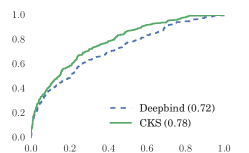
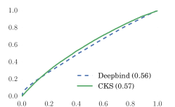
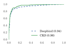
A)	B)	C)	D)

Figure 1: ROC of DeepBind and CKS for TFs EGR1 and ATF2 for GM12878. A) ROC for ATF2 on DeepBind’s test set. B) ROC for ATF2 on the ENCODE set. C) ROC for EGR1 on DeepBind’s test set. D) ROC for EGR1 on the ENCODE set.

We compare our CKS to DeepBind, a state-of-the-art CNN approach for predicting transcription factor (TF) binding sites. We compare to DeepBind over other CNN methods Zhou et al., (2015); Kelley et al., (2016) due to its primary attention to DNA sequence specificity and ability to identify fine grained (101 bp) locations of binding affinity.

3.1 Datasets

We train and evalute on datasets preprocessed from the ENCODE consortium. Because binding affinity is TF specific, we use separate train and evaluation sets for each TF.

We use the same training sets as DeepBind’s publically available models. We then evaluate on DeepBind’s test sets as well as a larger dataset processed directly from ENCODE.

DeepBind’s test sets consist of 1000 regions for each cell type over six TFs. Each set consists of 500 positive sequences extracted from regions of high ChIP-seq signal and 500 synthetic negative sequences generated from dinucleotide shuffle of positive sequences Alipanahi et al., (2015).

The second test dataset consists of 100,000 regions extracted from ChIP-seq datasets for TFs ATF2 and EGR1 across multiple cell types. Positive sequences are extracted from regions of high ChIP-seq signal. Negative sequences are extracted from regions of low ChIP-seq signal with exposed chromatin.

3.2 Experimental Setup

Experiments for DeepBind and CKS were run on one machine with 24 Xeon processors, and 256 GB of ram and 1 Nvidia Tesla K20c GPU.

We train a linear model minimizing squared loss with an L2 penalty of $\lambda$ on the output of the CKS defined in Algorithm 1. We do not tune the hyper-parameters $n$ (convolution size) and $M$ (number of kitchen sinks), and leave them constant at $8$ and $8192$ respectively. We tune the hyper paraemters $\gamma$ (kernel width) and $\lambda$ on held out data from the train set. To assess generalization across cellular contexts, we train and evaluate on separate cell types.

3.3 Evaluation

We compare DeepBind against CKS using area under the curve (AUC) of Receiver Operating Characteristic (ROC). We choose AUC as a metric for binary classifcation due to its ability to measure both TF binding site detection and false positive rates.

We detail our experimental results and compare to DeepBind’s pretrained models in Tables 1 and 2. We also show ROCs for ATF2 and EGR1 on both datasets in Figure 1.

Our AUC is competitive (within 0.01) or superior to that of DeepBind except for ATF2 on MCF7 cell type. Furthermore on five out of six large ENCODE test sets, our AUC is strictly greater than DeepBind.

We measure DeepBind’s training time on TF EGR1, trained on K562 with $72,996$ train sequences. DeepBind’s training procedure takes $6497$ seconds to learn $2123$ parameters. For comparison, training time for CKS takes $712$ seconds (Table 1) to learn $16384$ parameters, which is approximately eight times faster than DeepBind’s runtime.

4 Conclusion and Future Work

In this paper, we show that Convolutional Kitchen Sinks train eight times faster and has superior predictive performance to CNNs. We note that our current work focuses on binding affinity in the context of DNA sequence, making this model agnostic to specific cell contexts of interest. Because Algorithm 1 is not specific to DNA sequence, positional counts of chromatin accessibility and gene expression data can be aggregated with current implementation to account for cell type specific information. We leave this extension for future work.

References

- ENCODE et al., [2004] ENCODE Project Consortium and others. The ENCODE (Encyclopedia of DNA elements) project. In Science, volume 306, pages 636–640, 2004.
- Jaakola et al., [1999] Tommi S Jaakkola, Mark Diekhans, and David Haussler. Using the fisher kernel method to detect remote protein homologies. In ISMB, volume 99, pages 149–158, 1999.
- Eskin et al., [2002] Eleazar Eskin, Jason Weston, William S Noble, and Christina S Leslie. Mismatch string kernels for svm protein classification. In Advances in neural information processing systems, pages 1417–1424, 2002.
- Leslie et al., [2002] Christina S Leslie, Eleazar Eskin, and William Stafford Noble. The spectrum kernel: A string kernel for svm protein classification. In Pacific symposium on biocomputing, volume 7, pages 566–575, 2002.
- Fletez-Brant et al., [2013] Christopher Fletez-Brant, Dongwon Lee, Andrew S McCallion, and Michael A Beer. kmer-svm: a web server for identifying predictive regulatory sequence features in genomic data sets. Nucleic acids research, 41(W1):W544–W556, 2013.
- Lee et al., [2015] Dongwon Lee, David U Gorkin, Maggie Baker, Benjamin J Strober, Alessandro L Asoni, Andrew S McCallion, and Michael A Beer. A method to predict the impact of regulatory variants from dna sequence. Nature genetics, 47(8):955–961, 2015.
- Zhou et al., [2015] Jian Zhou and Olga G Troyanskaya. Predicting effects of noncoding variants with deep learning-based sequence model. Nature methods, 12(10):931–934, 2015.
- Alipanahi et al., [2015] Babak Alipanahi, Andrew Delong, Matthew T Weirauch, and Brendan J Frey. Predicting the sequence specificities of dna-and rna-binding proteins by deep learning. Nature biotechnology, 2015.
- Kelley et al., [2016] David R Kelley, Jasper Snoek, and John L Rinn. Basset: Learning the regulatory code of the accessible genome with deep convolutional neural networks. Genome research, 2016.
- Rahimi et al., [2007] Ali Rahimi and Benjamin Recht. Random features for large-scale kernel machines. In Advances in neural information processing systems, pages 1177–1184, 2007.
- Mairal et al., [2014] Julien Mairal, Piotr Koniusz, Zaid Harchaoui, and Cordelia Schmid. Convolutional kernel networks. In Advances in Neural Information Processing Systems, pages 2627–2635, 2014.
- Rahimi et al., [2009] Ali Rahimi and Benjamin Recht. Weighted sums of random kitchen sinks: Replacing minimization with randomization in learning. In Advances in neural information processing systems, pages 1313–1320, 2009.
- Ghandi et al., [2014] Mahmoud Ghandi, Dongwon Lee, Morteza Mohammad-Noori, and Michael A Beer. Enhanced regulatory sequence prediction using gapped k-mer features. PLoS Comput Biol, 10(7):e1003711, 2014.