Probabilistic response and rare events in Mathieu’s equation under correlated parametric excitation

Abstract

We derive an analytical approximation to the probability distribution function (pdf) for the response of Mathieu’s equation under parametric excitation by a random process with a spectrum peaked at the main resonant frequency, motivated by the problem of large amplitude ship roll resonance in random seas. The inclusion of random stochastic excitation renders the otherwise straightforward response to a system undergoing intermittent resonances: randomly occurring large amplitude bursts. Intermittent resonance occurs precisely when the random parametric excitation pushes the system into the instability region, causing an extreme magnitude response. As a result, the statistics are characterized by heavy-tails. We apply a recently developed mathematical technique, the probabilistic decomposition-synthesis method, to derive an analytical approximation to the non-Gaussian pdf of the response. We illustrate the validity of this analytic approximation through comparisons with Monte-Carlo simulations that demonstrate our result accurately captures the strong non-Gaussianity of the response.

1 Introduction

Parametrically forced systems arise in many engineering systems and natural phenomena. For such systems, parametric (subharmonic) resonance can produce a large response even when the parametric excitation amplitude is small. To investigate these ideas, parametric resonance has been extensively studied using the classic Mathieu’s equation and the more general Hill’s equation,

$$\ddot{x}(t)+(\omega_{0}^{2}+\varepsilon\Omega^{2}\sin(\Omega t))x(t)=0,$$ (1)

since it represents the typical response of a system when excited by a time periodic force. When the system’s natural frequency and the excitation frequency are near the ratio $\omega_{0}\,{:}\,\Omega=n\,{:}\,2,$ for positive integers $n$, the parametric resonance phenomena is important and we have regions of instabilities (fig. 1). The most prominent resonance region occurs for $n=1$ with the ratio $1\,{:}\,2$. Equation 1 is a simple, deterministic system that is often used to model the typical effect of parametric excitations that are time periodic or nearly time periodic. However, this is only a special case of more typical aperiodic time variations; indeed, in many physical systems, the induced excitations are inherently random (e.g. ship motions in random water waves [1, 2, 3, 4], modes in turbulence [5, 6, 7], and beam buckling due to random axial and lateral forcing [8, 9]). This randomness can significantly alter the system response, and in certain parametric regimes leads to transient instabilities and intermittent bursts of extreme magnitude. These events are directly connected with the finite correlation time of the excitation processes, and therefore cannot be quantified using deterministic analysis or approximations of the excitation processes by white-noise.

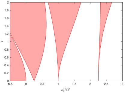
Figure 1: Ince-Strutt diagram showing the classical resonance tongues (shaded) for particular combinations of $\varepsilon$ and $\omega_{0}^{2}/\Omega^{2}$, for Mathieu’s equation 1. Transition frequencies at $\omega_{0}^{2}/\Omega^{2}=(n/2)^{2}$. Stability boundaries are computed using Hill’s infinite determinant approach [10].

1.1 Motivation

One important parametrically excited system in ocean engineering, and our motivating example, is ship rolling in the presence of random seas [11, 1, 2, 3, 4, 12, 13]. The first modern theoretical description of parametric rolling was given in [14] and the first experimental observation of the phenomenon in [15]. For ship rolling, the parametric resonance phenomena is a considerable threat to the safety of a vessel. Indeed, ever since the investigation into the post-Panamax C11 class cargo ship accident on October 20th, 1998, which was confirmed to have undergone severe roll motions in head seas during a storm, causing extensive loss and damage to the vessel (see [16] for details), interest in the problem has been renewed. This has lead to developments of important guidelines and criteria assessing the risk and susceptibility of vessels to roll motions [17]. As such, the problem of parametric rolling has been an important factor in the present debate on the second generation intact stability criteria (see [18] for the current status of the IMO criteria on rolling).

It is now well understand that large amplitude roll motions can occur through parametric resonance, even when there are no direct wave-induced roll moments. This is most prominent in head or following seas, where roll-restoring characteristics can vary significantly in time compared to still water conditions. When a wave crest is amid-ship, stability is reduced as the bow and stern are likely to have emerged, which reduce roll-restoring moments. The effects are most pronounced for wave lengths comparable to the ship length and increase for steeper waves.

The roll motion of a ship in following or head seas, for small pitch and heave motions, can be modeled by,

$$I\ddot{\phi}(t)+B(\dot{\phi}(t))+\Delta GZ(\phi(t))=F(t),$$ (2)

where $\phi(t)$ is the roll angle, $I$ is the inertia term including added mass, $B(\dot{\phi}(t))$ is the damping moment, $F(t)$ is a small wave excitation term, and $\Delta GZ(\phi(t))$ is the restoring moment term. The time-dependent restoring moments in irregular seas may, sometimes, be approximated by (see e.g. [11, 4])

$$\Delta GZ(\phi(t))=(\alpha+\xi(t))\phi(t)-\beta\phi^{3}(t),$$ (3)

where $\xi(t)$ is the random wave excitation, with a narrowbanded spectrum $S_{\xi}(\omega)$ around a frequency $\Omega$; thus we expect the parametric resonance phenomena to be important when the encounter frequency $\Omega$ is roughly twice the natural natural frequency of rolling. In addition, $B(\dot{\phi}(t))$ is a nonlinear function of the roll velocity. Since our goal is to model the leading order probabilistic dynamics that occur due to the interaction of the random time-dependent restoring term and the vessel’s roll angle, we neglect the assumed small nonlinear terms in the restoring and damping moments:

$$\phi(t)+f\dot{\phi}(t)+(\alpha+\xi(t))\phi(t)=F(t);$$ (4)

this choice is motivated by the fact that stochastic roll resonance, in this context, is a consequence of the multiplicative excitation term, and not nonlinearities in the restoring or damping terms. However, it is worthwhile to remark on the theoretical nature of eq. 4; system nonlinearities are important in accurate models of ship rolling and play a role in modifying the instability zones [19]. The inclusion of the cubic term in the restoring moment would, for one, impact the underlying shape at the very tail ends of the response probability density function by suppressing their magnitude. Furthermore, the excitation in roll motion is coupled with pitch and heave motions, and this requires at least three degrees of freedom. Despite these remarks, the model in eq. 4 serves as a useful prototype system for analytical work investigating the complex heavy-tailed probabilistic properties of roll resonance in random seas; and is motivated by the desire in design to have simple and accurate analytic predictors of dynamic stability that account for extreme conditions [20].

This summarizes the basic equation that govern the leading-order ship roll dynamics in the presence of irregular seas. Finally, we note the following: in certain parametric regimes, solutions of eq. 4 exhibit random periods of large amplitude roll motions (intermittency). It is this parametric regime we are interested in investigating here.

1.2 Stochastic generalization of Mathieu’s equation

While Mathieu’s equation and its variants have been extensively analyzed [21, 10], generalizations incorporating stochasticity are less well understood, but have been studied in various contexts [22, 9, 23, 24, 25]. A very important dynamical transition that occurs in the presence of random parametric forcing is intermittent resonance; that is, randomly occurring short-lived periods when the system experience parametric resonance. Deterministic models based on some time-averaged property of the noise would fail to capture this important dynamical transition, since this is an essentially transient phenomena.

To explore the effects of noise in parametric forcing, motivated by section 1.1, we consider the following generalization of eq. 1:

$$\ddot{x}(t)+2\zeta\omega_{0}\dot{x}(t)+\omega_{0}^{2}(1+\kappa(t))x(t)=F(t),$$ (5)

where $\kappa(t)$ is a narrowbanded random process, $F(t)$ is a broadbanded forcing term of low intensity, e.g. white noise, and $\zeta$ is the damping coefficient. For example, $\kappa(t)$ can be thought of as $\kappa(t)=\alpha(t)\sin(\Omega t)$, with frequency ratio near one of the resonance regions and $\alpha(t)$ a random process, such that the dominant energy in the spectrum $S_{\kappa}(\omega)$ is concentrated near $\Omega$; in other words, the noise has a dominant frequency component at $\Omega$. We explain later in detail the motivation behind this selection, for now we note that this spectrum follows quite naturally when modeling physical processes, in particular, random seas.

1.3 Perspective

Our goal here is to derive an analytical approximation to the probability density function (pdf) for the generalized Mathieu’s equation in eq. 5 when forced parametrically by a correlated random process near the principal resonance region; in particular, we are interested in the stationary probability distribution of the response in the regime undergoing intermittency. As mentioned, this is challenging since the system exhibits transient resonance, which can be identified by large amplitude spikes in the time-series of the response; as a result of intermittency, the resulting pdf is non-Gaussian with heavy-tailed characteristics. Recently, there have been efforts to quantify the heavy-tailed statistical structures for systems undergoing intermittent instabilities [26, 27, 6, 7]. Here, we apply a recently developed technique designed to approximate the pdf of systems exhibiting intermittent instabilities: the probabilistic decomposition-synthesis method [27, 26]. Since the system we investigate is low-dimensional, with linear damping and restoring terms, we apply the formulation in [26] to approximate the probability measure of the response. This approach provides us with analytical results, taking into account the correlated nature of the multiplicative excitation process $\kappa(t)$.

The benefits of this approach are numerous. For systems, such as in eq. 4, we can derive analytical results for the non-Gaussian response pdf, for both the main probability mass and the heavy-tailed structure. For systems where nonlinearities are important, we can adapt the method and apply the probabilistic decomposition-synthesis method in a computational setting, as described in [27], for a fast approximation of the response pdf that accounts for system nonlinearities.

While several methods can be applied to solve for the stationary measure for systems excited by multiplicative noise, for the case of transient instabilities, as might occur in parametric rolling 4, they are severely limited in practicality due to their large computational demands and/or limitations in dealing with the strongly transient nature of intermittent instabilities. For example, the Monte-Carlo approach (direct sampling of long time realizations of the system), while very attractive since it provides the most accurate results, is a very computationally intensive procedure, requiring many realizations for accurately resolved tail statistics. Another technique is to formulate the associated Fokker-Planck-Kolmogorov (FPK) equation for eq. 5 [28]. This can be performed by utilizing shape filtering to approximate the correlated excitation process. However, using filtered Gaussian white noise is prone to introduce significant errors in the tails of the response (even small numerical errors in time-series simulations of $\kappa(t)$ lead to large inaccuracies in the tail statistics of $x(t)$ [29]). In any case, this approach requires solving a demanding FPK equation [30], which also has to be done to high accuracy (tail events have extremely low probabilities).

Stochastic averaging is another widely used method [31]; the typical approach here would be to first derive a set of equations for the slowly varying variables and then to apply the stochastic averaging procedure to arrive at a set of Itō stochastic differential equations for the transformed coordinates. The Fokker-Plank-Kolmogorov equation can then be used to solve for the response pdf [9, 32]. Clearly, this approach is not valid in parametric regimes undergoing intermittent resonance, since it averages away the time dependent nature of the multiplicative excitation, leading to Gaussian statistics, which is decidedly not the case.

1.4 Outline

In section 2 we formulate the problem and provide the problem statement; we explain the particular form of the excitation noise structure and its interaction with the system dynamics in the parametric regime of interest. Following this discussion, in section 3, we derive equations that govern the slow dynamics of the problem. The equations for the slowly varying variables are the starting point of our application of the probabilistic decomposition-synthesis method, which we briefly give an overview in section 4. In section 5 we apply the method to derive the analytical formula that approximates the pdf of Mathieu’s equation in the parametric regime of interest, and in section 6 we compare the analytical formula with numerical results from Monte-Carlo simulations.

2 Problem formulation

We consider the following stochastic generalization of Mathieu’s equation:

$$\ddot{x}(t)+2\zeta\omega_{0}\dot{x}(t)+\omega_{0}^{2}(1+\kappa(t))x(t)=F(t),$$ (6)

where $\omega_{0}$ is the undamped natural frequency of the system, $\zeta$ is the damping coefficient, $\kappa(t)$ is a narrowbanded random process around $\Omega$, and $F(t)$ is an additive broadbanded random excitation term; we assume both $\kappa(t)$ and $F(t)$ are stationary Gaussian processes.

As mentioned, the deterministic form of Mathieu’s equation,

$$\ddot{x}(t)+2\zeta\omega_{0}\dot{x}(t)+\omega_{0}^{2}(1+\alpha\sin\Omega t)x(t)=0,$$ (7)

has unstable solutions depending upon the parametric excitation frequency $\Omega$ and amplitude $\alpha$ parameters. Near $\Omega/2\omega_{0}=1/n$, for positive integers $n$, we have regions of instabilities, with the widest instability region being for $n=1$. Damping has the effect of raising the instability regions from the $\Omega/2\omega_{0}$ axis by $2(2\zeta)^{1/n}$. Therefore, for $\zeta\ll 1$ the instability region near $n=1$ is of greatest practical importance [9, 10].

Furthermore, since we are interested in analyzing the response pdf in the regime where the system is undergoing intermittent resonance, we assume $\kappa(t)$ is a narrowbanded random process around the most important resonant region at frequency $\Omega=2\omega_{0}$. The approach can be extended if the frequency is detuned, but for simplicity of the presentation we consider no detuning. In this case, intermittent resonance is a possibility since the stochastic process $\kappa(t)$ may randomly cross into the instability tongue. In other words, for the regime of interest, on average $\kappa(t)$ is in a state such that the variance of the response $x(t)$ is associated with the background attractor, however with low probability $\kappa(t)$ can transition to a critical regime, producing an intermittently unstable response of severe magnitude. Thus, through this regime switching, we have randomly occurring periods of large amplitude responses, which are finite-time instabilities with positive Lyapunov exponent; a typical time-series is shown in fig. 2. The severity of these instabilities depends upon the magnitude of the damping term and the amplitude and characteristic time-scale of the multiplicative noise term.

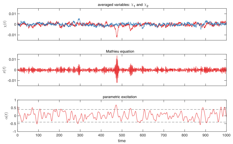
Figure 2: Sample realization of Mathieu’s equation (middle, eq. 8) under the prarametric excitation term (bottom) and the corresponding averaged variables $\chi_{1}$ and $\chi_{2}$ (top, eqs. 16 and 17). The random amplitude forcing term $\alpha(t)$ triggers intermittent resonance when it crosses above or below the instability thresholds (dashed lines).

2.1 Excitation process

For concreteness we assume the excitation process takes a canonical form $\kappa(t)=\alpha(t)\sin(2\omega_{0}t)$, where $\alpha(t)$ is a stationary Gaussian process with a non-oscillatory correlation function. Additionally, $\mkern 1.0mu\overline{\mkern-1.0mu\alpha(t)\mkern-1.0mu}\mkern 1.0mu=0$ and $R(\tau)=\mkern 1.0mu\overline{\mkern-1.0mu\alpha(t)\alpha(t+\tau)\mkern-1.0mu}\mkern 1.0mu=\sigma_{\alpha}^{2}e^{-\tau^{2}/2\ell_{\alpha}^{2}}$, where $\ell_{\alpha}$ is the characteristic time-scale of the process and $\sigma_{\alpha}^{2}$ its variance.

Problem statement

With these considerations, the problem is to derive an approximation for the stationary probability distribution for the system:

$$\ddot{x}(t)+2\zeta\omega_{0}\dot{x}(t)+\omega_{0}^{2}(1+\alpha(t)\sin(2\omega_{0}t))x(t)=F(t),$$ (8)

in the parametric regime undergoing intermittent resonance. The final result is given in eq. 44.

3 Derivation of the slow dynamics

We proceed by assuming a narrow band response around $\omega_{0}$ and averaging over this fast frequency the governing system 8. By introducing the coordinate transformation

$$x(t) =\chi_{1}(t)\cos(\omega_{0}t)+\chi_{2}(t)\sin(\omega_{0}t),$$ (9)

$$\dot{x}(t) =-\omega_{0}\chi_{1}(t)\sin(\omega_{0}t)+\omega_{0}\chi_{2}(t)\cos(\omega_{0}t),$$

in eq. 8 and using the additional relation $\dot{\chi}_{1}(t)\cos(\omega_{0}t)+\dot{\chi}_{2}(t)\sin(\omega_{0}t)=0$, we obtain the following pair of equations for the slow variables $\chi_{1}(t)$ and $\chi_{2}(t)$:

$$\begin{multlined}\dot{\chi}_{1}=-\biggl{[}2\zeta\omega_{0}\biggl{(}\chi_{1}\sin^{2}(\omega_{0}t)-\frac{1}{2}\chi_{2}\sin(2\omega_{0}t)\biggr{)}-\frac{\omega_{0}\alpha}{2}\chi_{1}\sin^{2}(2\omega_{0}t)\\ -\omega_{0}\alpha\chi_{2}\sin^{2}(\omega_{0}t)\sin(2\omega_{0}t)\biggr{]}-\frac{1}{\omega_{0}}\sin(\omega_{0}t)F(t),\end{multlined}\dot{\chi}_{1}=-\biggl{[}2\zeta\omega_{0}\biggl{(}\chi_{1}\sin^{2}(\omega_{0}t)-\frac{1}{2}\chi_{2}\sin(2\omega_{0}t)\biggr{)}-\frac{\omega_{0}\alpha}{2}\chi_{1}\sin^{2}(2\omega_{0}t)\\ -\omega_{0}\alpha\chi_{2}\sin^{2}(\omega_{0}t)\sin(2\omega_{0}t)\biggr{]}-\frac{1}{\omega_{0}}\sin(\omega_{0}t)F(t),$$ (12)

$$\begin{multlined}\dot{\chi}_{2}=\biggl{[}2\zeta\omega_{0}\biggl{(}\frac{1}{2}\chi_{1}\sin(2\omega_{0}t)-\chi_{2}\cos^{2}(\omega_{0}t)\biggr{)}-\frac{\omega_{0}\alpha}{2}\chi_{2}\sin^{2}(2\omega_{0}t)\\ -\omega_{0}\alpha\chi_{1}\cos^{2}(\omega_{0}t)\sin(2\omega_{0}t)\biggr{]}+\frac{1}{\omega_{0}}\cos(\omega_{0}t)F(t).\end{multlined}\dot{\chi}_{2}=\biggl{[}2\zeta\omega_{0}\biggl{(}\frac{1}{2}\chi_{1}\sin(2\omega_{0}t)-\chi_{2}\cos^{2}(\omega_{0}t)\biggr{)}-\frac{\omega_{0}\alpha}{2}\chi_{2}\sin^{2}(2\omega_{0}t)\\ -\omega_{0}\alpha\chi_{1}\cos^{2}(\omega_{0}t)\sin(2\omega_{0}t)\biggr{]}+\frac{1}{\omega_{0}}\cos(\omega_{0}t)F(t).$$ (15)

Averaging the deterministic terms in brackets over the fast frequency in eqs. 12 and 15 gives,

$$\dot{\chi}_{1}(t) =-\biggl{(}\zeta-\frac{\alpha(t)}{4}\biggr{)}\omega_{0}\chi_{1}(t)-\frac{1}{\omega_{0}}\sin(\omega_{0}t)F(t),$$ (16)

$$\dot{\chi}_{2}(t) =-\biggl{(}\zeta+\frac{\alpha(t)}{4}\biggr{)}\omega_{0}\chi_{2}(t)+\frac{1}{\omega_{0}}\cos(\omega_{0}t)F(t).$$ (17)

The equations above for the slow variables provide good pathwise and statistical agreement with eq. 8. Furthermore, these equations make it clear that an instability is expected when $\lvert\alpha(t)\rvert>4\zeta$ (shown in dashed lines in fig. 2); this instability criterion is nothing more than the well-known instability condition of the deterministic case (for fixed in time $\alpha$), which to leading order is given by: $\delta=1/4\pm 1/2\sqrt{\alpha^{2}\delta^{2}-4\zeta^{2}\delta}$, where $\delta=\omega_{0}^{2}/\Omega^{2}$ (see left plot in fig. 3)

Next, we apply a stochastic averaging procedure to the additive forcing term, also known as the diffusion approximation [9, 33, 34]. More specifically, if the governing dynamics act on a sufficiently slower time scale than the memory of the additive stochastic process, then the independent increment approximation is valid. This is the case if the stochastic process $F(t)$ is broadbanded, and leads to the following set of Itō stochastic differential equations for the slow variables:

$$\dot{\chi}_{1}(t) =-\biggl{(}\zeta-\frac{\alpha(t)}{4}\biggr{)}\omega_{0}\chi_{1}(t)+\sqrt{2\pi K}\,\dot{W}_{1}(t),$$ (18)

$$\dot{\chi}_{2}(t) =-\biggl{(}\zeta+\frac{\alpha(t)}{4}\biggr{)}\omega_{0}\chi_{2}(t)+\sqrt{2\pi K}\,\dot{W}_{2}(t),$$ (19)

with $K=S_{F}(\omega_{0})/2\omega_{0}^{2}$, where $S_{F}(\omega_{0})$ is the spectral density of the additive excitation $F(t)$ at frequency $\omega_{0}$, and $\dot{W}_{1}$ and $\dot{W}_{2}$ are independent white noise processes of unit intensity [9]. The slowly varying variables, after averaging the forcing term, transform to two decoupled stochastic differential equations. Equations 18 and 19 are a good statistical approximation to the original system 8 (but provide poor pathwise agreement).

We emphasize that the broadband hypothesis for the additive stochastic process is a convenient setup that leads to the derived white-noise formulation. However, the analysis and results that follow do not require the white-noise formulation and are directly applicable for the general case of an (non white-noise) additive stochastic forcing. Such a case could be, for example, an additive narrowbanded forcing term with spectral content distributed around $\omega_{0}$.

4 The probabilistic decomposition-synthesis method

The analysis in section 2 provides the dynamics of the slow variables and reveals the interaction of the parametric excitation process $\alpha(t)$ with the slow variables. Starting from these equations we can apply the probabilistic decomposition-synthesis method to analytically approximate the stationary measure of $\chi(t)$. To be self-contained, we provide a very brief overview of the probabilistic decomposition-synthesis method adapted to the current problem; further details can be found in [26] and a detailed description of the method in a general context in [27].

The main idea of the method is to decompose the system response as:

$$x(t)=x_{b}(t)+x_{r}(t),$$ (20)

where $x_{r}$ is the solution when a rare event due to an instability occurs and $x_{b}$ is the stochastic response otherwise, i.e. the background dynamics. To be more specific $x_{r}$ will be the response of the system when the following two conditions are satisfied: (i) $\lVert x\rVert>\zeta$, where $\zeta$ is the extreme event threshold with respect to a chosen norm $\lVert\,\cdot\,\rVert$, and (ii) the parametric excitation obtains values that lead to an instability, i.e. $\alpha(t)\in R_{e}$, where $R_{e}$ describes the critical region of values for $\alpha(t)$ that induce an instability.

Together with this decomposition into rare events and the stochastic background, we also adopt the following assumptions:

1. The existence of intermittent events has negligible effect on the statistical characteristics of the stochastic attractor and can be ignored when analyzing the background state $x_{b}$;

2. Rare events are statistically independent from each other.

With this setup we can analyze the two states separately and probabilistically synthesize the information obtained from this analysis. This is completed using a total probability argument to obtain the statistics for an arbitrary quantity of interest $q$ by

$$\operatorname{\rho}(q)=\operatorname{\rho}(q\mid{\lVert x\rVert>\zeta,\alpha\in R_{e}})\operatorname{\mathbb{P}}_{r}+\operatorname{\rho}(q\mid x=x_{b})(1-\operatorname{\mathbb{P}}_{r}).$$ (21)

In this paper, the quantity of interest is the system response $x$. The first term expresses the contribution of rare events due to instabilities and is the heavy-tailed portion of the distribution for $q$ and the second term expresses the contribution of the background state, which contributes the main probability mass in the pdf for $q$. Moreover, $\operatorname{\mathbb{P}}_{r}\equiv\operatorname{\mathbb{P}}(\lVert x\rVert>\zeta,\alpha\in R_{e})$ is the total probability of a rare event, which is defined as the ratio between the time the system spends in rare event responses over the total time. Note that the temporal duration of rare transitions also includes a decay or relaxation phase to the background attractor, where the instability is no longer active but the system response still has important magnitude.

5 The probability distribution for the response

Here we apply the various steps of the probabilistic decomposition-synthesis method to derive analytical results that approximate the heavy-tailed distribution of the response for the system in eq. 8. In particular, we apply the method directly on the slow variables, since the fast frequency we averaged over is inconsequential in the pdf of the response.

Firstly, because $\alpha(t)$ is a zero mean process both $\chi_{1}(t)$ and $\chi_{2}(t)$ follow the same probability distribution. Consider the following equation that represents the slowly varying variables:

$$\dot{\chi}(t)=-\biggl{(}\zeta-\frac{\alpha(t)}{4}\biggr{)}\omega_{0}\chi(t)+\sqrt{2\pi K}\,\dot{W}(t)$$ (22)

We write eq. 22 as

$$\dot{\chi}(t)=-\gamma(t)\chi(t)+\sigma_{F}\,\dot{W}(t),$$ (23)

where $\sigma_{F}=\sqrt{2\pi K}$ and $\gamma(t)=\zeta\omega_{0}-\omega_{0}\alpha(t)/4$ is a Gaussian process with mean $\zeta\omega_{0}$ and standard deviation $\sigma_{\alpha}\omega_{0}/4$. Equation 23 will be the starting point for the application of the decomposition-synthesis method.

5.1 Decomposition and the instability region

Equation 23 makes it clear that intermittency is due to the parametric forcing term $\gamma(t)$ switching signs from positive to negative values. This sign switching causes $\chi(t)$ to transition from its regular response to a domain where the likelihood of an instability is high. This switching in $\gamma(t)$ is the mechanism behind instabilities in the variable $\chi(t)$. Therefore, we define the instability region as

$$R_{e}\coloneqq\{\gamma(t)\mid\gamma(t)<0\}.$$ (24)

In addition, for convenience, we define an instability threshold by $\eta\coloneqq 4\zeta/\sigma_{\alpha}$, the ratio of the mean over the standard deviation of the process $\gamma$.

5.2 Conditional distribution of the background dynamics

In the background state $R_{e}^{c}$, by definition, we have no rare events. We can approximate the background dynamics by replacing $\gamma(t)$ with its average value in this regime. The conditional average of $\gamma(t)$ in $R_{e}^{c}$ is

$$\mkern 1.0mu\overline{\mkern-1.0mu\gamma\mkern-1.0mu}\mkern 1.0mu|_{\gamma>0}=\zeta\omega_{0}+\frac{\sigma_{\alpha}\omega_{0}}{4}\frac{\phi(\eta)}{\Phi(\eta)},$$ (25)

where $\phi(\,\cdot\,)$ is the normal probability density function and $\Phi(\,\cdot\,)$ is the normal cumulative distribution function; thus the background dynamics is described by the Ornstein-Uhlenbeck process:

$$\dot{\chi}(t)=-\mkern 1.0mu\overline{\mkern-1.0mu\gamma\mkern-1.0mu}\mkern 1.0mu|_{\gamma>0}\chi(t)+\sigma_{F}\,\dot{W}(t).$$ (26)

Now the dynamics are globally stable in $R_{e}^{c}$ and we can directly obtain the stationary distribution for eq. 26:

$$\operatorname{\rho}_{\chi}(\chi\mid R_{e}^{c})=\sqrt{\frac{\mkern 1.0mu\overline{\mkern-1.0mu\gamma\mkern-1.0mu}\mkern 1.0mu|_{\gamma>0}}{\pi\sigma_{F}^{2}}}\exp\biggl{(}{-\frac{\mkern 1.0mu\overline{\mkern-1.0mu\gamma\mkern-1.0mu}\mkern 1.0mu|_{\gamma>0}}{\sigma_{F}^{2}}}\chi^{2}\biggr{)},$$ (27)

which is Gaussian distributed. To formulate our result in terms of the system variable $x$, we refer to the narrowbanded approximation made when averaging the governing system 8. This gives, approximately, $x=\chi\cos\varphi,$ where $\varphi$ is a uniform random variable distributed between 0 and $2\pi$. The probability density function for $z=\cos\varphi$ is given by $\operatorname{\rho}_{z}(z)=1/(\pi\sqrt{1-z^{2}}),$ $z\in[-1,1].$ To avoid additional integrations for the computation of the pdf, we approximate the distribution for $z$ by $\operatorname{\rho}_{z}(z)=\frac{1}{2}(\delta(z+1)+\delta(z-1)).$ This gives the following approximation for the background statistics

$$\operatorname{\rho}(x\mid R_{e}^{c})=\operatorname{\rho}_{\chi}(x\mid R_{e}^{c})=\sqrt{\frac{\mkern 1.0mu\overline{\mkern-1.0mu\gamma\mkern-1.0mu}\mkern 1.0mu|_{\gamma>0}}{\pi\sigma_{F}^{2}}}\exp\biggl{(}{-\frac{\mkern 1.0mu\overline{\mkern-1.0mu\gamma\mkern-1.0mu}\mkern 1.0mu|_{\gamma>0}}{\sigma_{F}^{2}}}x^{2}\biggr{)}.$$ (28)

Therefore, the conditional distribution of the background dynamics is Gaussian distributed.

5.3 Conditional distribution of rare events

Here we derive the conditional distribution of the response when an instability occurs. We characterize localized instabilities by a growth phase, corresponding directly to $\gamma(t)<0$, and a relaxation phase that brings the system back to the background state; both phases follow the same distribution [26]. Additionally, during the occurrence of an instability we neglect additive excitation and damping, and approximate the magnitude of the envelope as $\xi\equiv|\chi|\ \simeq\xi_{0}e^{\Lambda T_{\gamma<0}}$, where $\xi_{0}$ is the magnitude of the position’s envelope, $|\chi_{0}|$ right before the instability has begun to emerge, $\Lambda$ is a random variable that represents the Lyapunov exponent, and $T_{\gamma<0}$ is the random length of time that the process $\gamma$ spends below the zero level.

We first determine the statistical characteristics of $\Lambda$ and $T_{\gamma<0}$ (which we assume are independent). By substituting the representation $\xi\equiv|\chi|\simeq|\chi_{0}|e^{\Lambda T_{\gamma<0}}$ into eq. 23 we obtain $\Lambda=-\gamma$ so that

$$\operatorname{\rho}_{\Lambda}(\lambda)=\operatorname{\mathbb{P}}(-\gamma\mid\gamma<0)=\frac{4}{\sigma_{\alpha}\omega_{0}(1-\Phi(\eta))}\phi\biggl{(}4\frac{\lambda+\zeta\omega_{0}}{\sigma_{\alpha}\omega_{0}}\biggr{)}.$$ (29)

The distribution of the duration of time the process $\gamma(t)$ spends below an arbitrary threshold level $\eta$ is not in general available. However, one can show that the asymptotic expression in the limit of rare crossings, $\eta\to\infty$, is [35]

$$\operatorname{\rho}_{T_{\gamma<0}}(t)=\frac{\pi t}{2\mkern 1.0mu\overline{\mkern-1.0muT\mkern-1.0mu}\mkern 1.0mu^{2}}e^{-\pi t^{2}/4\mkern 1.0mu\overline{\mkern-1.0muT\mkern-1.0mu}\mkern 1.0mu^{2}},$$ (30)

and in our case this is a good approximation since we assume instabilities are rare events. In eq. 30 $\mkern 1.0mu\overline{\mkern-1.0muT\mkern-1.0mu}\mkern 1.0mu$ represents the average length of an instability, which for a Gaussian process is given by the ratio between the probability of $\gamma<0$ and the average number of downcrossings of the zero level per unit time $\mkern 1.0mu\overline{\mkern-1.0mu{N}^{-}_{\gamma}\mkern-1.0mu}\mkern 1.0mu(0)$ by $\gamma$ [35]

$$\mkern 1.0mu\overline{\mkern-1.0muT\mkern-1.0mu}\mkern 1.0mu=\frac{\operatorname{\mathbb{P}}(\gamma<0)}{\mkern 1.0mu\overline{\mkern-1.0mu{N}^{-}_{\gamma}\mkern-1.0mu}\mkern 1.0mu(0)}=\frac{1-\Phi(\eta)}{\frac{1}{2\pi}\sqrt{-R_{\alpha}^{\prime\prime}(0)}\exp(-\eta^{2}/2)},$$ (31)

where we have used Rice’s formula for the expected number of upcrossings [36] and $R_{\alpha}(\tau)$ is the correlation function of $\alpha(t)$ and $R_{\alpha}^{\prime\prime}(0)$ is the second derivative of the correlation function evaluated at $\tau=0$.

With these results we can determine the distribution of $\xi$ in $R_{e}$; the derived distribution is given by:

$$\operatorname{\rho}(\xi\mid\xi_{0},\alpha\in R_{e})=\frac{1}{\xi}\int\limits_{0}^{\infty}\frac{1}{y}\operatorname{\rho}_{\Lambda}(y)\operatorname{\rho}_{T}\biggl{(}\frac{\log(\xi/\xi_{0})}{y}\biggr{)}\,dy,\quad\xi>\xi_{0}.$$ (32)

Substituting in eqs. 29 and 30 gives,

$$\operatorname{\rho}(\xi\mid\xi_{0},\alpha\in R_{e})=\frac{2\pi\log(\xi/\xi_{0})}{\sigma_{\alpha}\omega_{0}\mkern 1.0mu\overline{\mkern-1.0muT\mkern-1.0mu}\mkern 1.0mu^{2}(1-\Phi(\eta))\xi}\int\limits_{0}^{\infty}\frac{1}{y^{2}}\phi\biggl{(}4\frac{y+\zeta\omega_{0}}{\sigma_{\alpha}\omega_{0}}\biggr{)}\exp{\bigg{(}-\frac{\pi}{4\mkern 1.0mu\overline{\mkern-1.0muT\mkern-1.0mu}\mkern 1.0mu^{2}y^{2}}\log(\xi/\xi_{0})^{2}\bigg{)}}\,dy,\quad\xi>\xi_{0}.$$ (33)

The variable $\xi_{0}$ corresponds to the magnitude of the background state $x_{b}$ before an instability occurs. Since, the background state is a narrowbanded Gaussian process, the magnitude of the envelope $\xi_{0}$ can be modeled as a Rayleigh distribution (see [37]) with scale parameter equal to the standard deviation of the Gaussian process 28.

Note, however, that in eq. 21 we are interested in the conditional statistics of events caused by instabilities which also have important magnitude. As described in [26], if the envelope’s magnitude when an instability occurs is small, then even though we have an instability we do not necessarily have a rare event, i.e. a response that is distinguishable from the typical background state response. This requires us to consider background states $\xi_{0}$, which are sufficiently large to result in a rare event $\lVert x\rVert>\zeta$. To this end, we consider only background states such that $\xi_{0}>\zeta=\sigma_{F}/\sqrt{2\mkern 1.0mu\overline{\mkern-1.0mu\gamma\mkern-1.0mu}\mkern 1.0mu|_{\gamma>0}}$, i.e. we consider extreme responses with magnitude at least one standard deviation of the background statistics when an instability also occurs. We emphasize that the exact choice for $\zeta$ plays little role on the approximation properties of the derived analytical expression. This requirement gives the final distribution for $\xi_{0}$,

$$\operatorname{\rho}_{\xi_{0}}(\xi_{0}\mid\xi_{0}>\zeta)=\frac{2\mkern 1.0mu\overline{\mkern-1.0mu\gamma\mkern-1.0mu}\mkern 1.0mu|_{\gamma>0}}{\sigma_{F}^{2}}(\xi_{0}-\zeta)\exp\biggl{(}-\frac{\mkern 1.0mu\overline{\mkern-1.0mu\gamma\mkern-1.0mu}\mkern 1.0mu|_{\gamma>0}}{\sigma_{F}^{2}}(\xi_{0}-\zeta)^{2}\biggr{)},\quad\xi_{0}>\zeta.$$ (34)

Using eq. 34 in eq. 33 we obtain

$$\operatorname{\rho}(\xi\mid\xi>\zeta,\alpha\in R_{e})=\int\operatorname{\rho}(\xi\mid\xi_{0},\alpha\in R_{e})\operatorname{\rho}_{\xi_{0}}(\xi_{0}\mid\xi_{0}>\zeta)\,d\xi_{0}.$$ (35)

In the last step, we transform the envelope representation back to the real variable $x$ through the same narrowbanded argument used in section 5.2 for the background state distribution; this gives the final result for the distribution of the rare event regime:

$$\operatorname{\rho}(x\mid\left\|x\right\|>\zeta,\alpha\in R_{e}) \simeq\frac{1}{2}\int\operatorname{\rho}(\left|x\right|\mid\xi_{0},\alpha\in R_{e})\operatorname{\rho}_{\xi_{0}}(\xi_{0}\mid\xi_{0}>\zeta)\,d\xi_{0},$$ (36)

$$\begin{multlined}=\frac{\sqrt{2\pi}\mkern 1.0mu\overline{\mkern-1.0mu\gamma\mkern-1.0mu}\mkern 1.0mu|_{\gamma>0}}{\sigma_{F}^{2}\sigma_{\alpha}\omega_{0}\ \mkern 1.0mu\overline{\mkern-1.0muT\mkern-1.0mu}\mkern 1.0mu^{2}(1-\Phi(\eta))}\int\limits_{\zeta}^{\lvert x\rvert}\!\int\limits_{0}^{\infty}\frac{\log(\lvert x\rvert/\xi_{0})}{y^{2}(\lvert x\rvert/(\xi_{0}-\zeta))}\exp\biggl{(}-8\frac{(y+\zeta\omega_{0})^{2}}{\sigma_{\alpha}^{2}\omega_{0}^{2}}\\ -\frac{\pi}{4\mkern 1.0mu\overline{\mkern-1.0muT\mkern-1.0mu}\mkern 1.0mu^{2}y^{2}}\log(\lvert x\rvert/\xi_{0})^{2}-\frac{\mkern 1.0mu\overline{\mkern-1.0mu\gamma\mkern-1.0mu}\mkern 1.0mu|_{\gamma>0}}{\sigma_{F}^{2}}(\xi_{0}-\zeta)^{2}\bigg{)}\,dy\,d\xi_{0},\end{multlined}=\frac{\sqrt{2\pi}\mkern 1.0mu\overline{\mkern-1.0mu\gamma\mkern-1.0mu}\mkern 1.0mu|_{\gamma>0}}{\sigma_{F}^{2}\sigma_{\alpha}\omega_{0}\ \mkern 1.0mu\overline{\mkern-1.0muT\mkern-1.0mu}\mkern 1.0mu^{2}(1-\Phi(\eta))}\int\limits_{\zeta}^{\lvert x\rvert}\!\int\limits_{0}^{\infty}\frac{\log(\lvert x\rvert/\xi_{0})}{y^{2}(\lvert x\rvert/(\xi_{0}-\zeta))}\exp\biggl{(}-8\frac{(y+\zeta\omega_{0})^{2}}{\sigma_{\alpha}^{2}\omega_{0}^{2}}\\ -\frac{\pi}{4\mkern 1.0mu\overline{\mkern-1.0muT\mkern-1.0mu}\mkern 1.0mu^{2}y^{2}}\log(\lvert x\rvert/\xi_{0})^{2}-\frac{\mkern 1.0mu\overline{\mkern-1.0mu\gamma\mkern-1.0mu}\mkern 1.0mu|_{\gamma>0}}{\sigma_{F}^{2}}(\xi_{0}-\zeta)^{2}\bigg{)}\,dy\,d\xi_{0},$$ (39)

5.4 Probability of rare events

Next we determine the total probability of rare events, that is the ratio of time that the system response spends in rare transitions over the total time, which we denote by $\operatorname{\mathbb{P}}_{r}$. This quantity can be computed by analyzing the duration of transitions into $R_{e}$, i.e. the duration of instabilities, but also including the time it takes for the response to return to the background attractor.

Consider a representative extreme event with an average growth rate $\mkern 1.0mu\overline{\mkern-1.0mu\Lambda\mkern-1.0mu}\mkern 1.0mu_{+}$ and decay rate $\mkern 1.0mu\overline{\mkern-1.0mu\Lambda\mkern-1.0mu}\mkern 1.0mu_{-}$. During the growth phase the dynamics are approximated by:

$$\xi_{p}=\xi_{0}\exp({\mkern 1.0mu\overline{\mkern-1.0mu\Lambda\mkern-1.0mu}\mkern 1.0mu_{+}T_{\gamma<0}}),$$ (40)

where $T_{\gamma<0}$ is the duration of the growth event and $\xi_{p}$ the peak value of the response. Similarly, over the decay phase:

$$\xi_{0}=\xi_{p}\exp({-\mkern 1.0mu\overline{\mkern-1.0mu\Lambda\mkern-1.0mu}\mkern 1.0mu_{-}T_{\text{decay}}}).$$ (41)

This gives that:

$$\frac{T_{\text{decay}}}{T_{\gamma<0}}=\frac{\mkern 1.0mu\overline{\mkern-1.0mu\Lambda\mkern-1.0mu}\mkern 1.0mu_{+}}{\mkern 1.0mu\overline{\mkern-1.0mu\Lambda\mkern-1.0mu}\mkern 1.0mu_{-}}=\frac{-\mkern 1.0mu\overline{\mkern-1.0mu\gamma\mkern-1.0mu}\mkern 1.0mu|_{\gamma<0}}{\mkern 1.0mu\overline{\mkern-1.0mu\gamma\mkern-1.0mu}\mkern 1.0mu|_{\gamma>0}}=\frac{-\zeta\ +\frac{\sigma_{\alpha}}{4}\frac{\phi(\eta)}{1-\Phi(\eta)}}{\zeta\ +\frac{\sigma_{\alpha}}{4}\frac{\phi(\eta)}{\Phi(\eta)}}\equiv\upsilon.$$ (42)

The average duration of rare transitions is thus given by $T_{e}=(1+\mkern 1.0mu\overline{\mkern-1.0mu\Lambda\mkern-1.0mu}\mkern 1.0mu_{+}/\mkern 1.0mu\overline{\mkern-1.0mu\Lambda\mkern-1.0mu}\mkern 1.0mu_{-})T_{\gamma<0}$. Dividing over the total length of time $T$, gives the final result for the probability of rare transitions:

$$\operatorname{\mathbb{P}}_{r}\simeq(1+\mkern 1.0mu\overline{\mkern-1.0mu\Lambda\mkern-1.0mu}\mkern 1.0mu_{+}/\mkern 1.0mu\overline{\mkern-1.0mu\Lambda\mkern-1.0mu}\mkern 1.0mu_{-})\operatorname{\mathbb{P}}(\gamma<0)=(1+\upsilon)(1-\Phi(\eta)).$$ (43)

5.5 Summary of the analytical results

With the analysis above, we synthesize the results by a total probability law argument:

$$\operatorname{\rho}_{x}(x)=(1-\operatorname{\mathbb{P}}_{r})\sqrt{\frac{\mkern 1.0mu\overline{\mkern-1.0mu\gamma\mkern-1.0mu}\mkern 1.0mu|_{\gamma>0}}{\pi\sigma_{F}^{2}}}\exp\biggl{(}\frac{-\mkern 1.0mu\overline{\mkern-1.0mu\gamma\mkern-1.0mu}\mkern 1.0mu|_{\gamma>0}}{\sigma_{F}^{2}}x^{2}\biggr{)}\\ +\operatorname{\mathbb{P}}_{r}\frac{\sqrt{2\pi}\mkern 1.0mu\overline{\mkern-1.0mu\gamma\mkern-1.0mu}\mkern 1.0mu|_{\gamma>0}}{\sigma_{F}^{2}\sigma_{\alpha}\omega_{0}\ \mkern 1.0mu\overline{\mkern-1.0muT\mkern-1.0mu}\mkern 1.0mu^{2}(1-\Phi(\eta))}\int\limits_{\zeta}^{\lvert x\rvert}\!\int\limits_{0}^{\infty}\frac{\log(\lvert x\rvert/\xi_{0})}{y^{2}(\lvert x\rvert/(\xi_{0}-\zeta))}\\ \times\exp\biggl{(}-8\frac{(y+\zeta\omega_{0})^{2}}{\sigma_{\alpha}^{2}\omega_{0}^{2}}-\frac{\pi}{4\mkern 1.0mu\overline{\mkern-1.0muT\mkern-1.0mu}\mkern 1.0mu^{2}y^{2}}\log(\lvert x\rvert/\xi_{0})^{2}-\frac{\mkern 1.0mu\overline{\mkern-1.0mu\gamma\mkern-1.0mu}\mkern 1.0mu|_{\gamma>0}}{\sigma_{F}^{2}}(\xi_{0}-\zeta)^{2}\bigg{)}\,dy\,d\xi_{0},$$ (44)

where the integral is zero for $\lvert x\rvert<\zeta$. Note that $\sigma_{F}^{2}=\pi S_{F}(\omega_{0})/\omega_{0}^{2}$ for the case of a broadbanded additive excitation and $\sigma_{F}^{2}=\nu^{2}/2\omega_{0}^{2}$ for the case of a white noise additive excitation with intensity $\nu$ (i.e. $F(t)=\nu\dot{W}(t)$).

We emphasize that eq. 44 is a heavy-tailed and symmetric probability measure (non-negative and integrates to one). In fig. 3 we present the stability diagram for constant (in time) $\alpha$ and for finite damping $\zeta=0.1$ (red shaded region in the left plot). For the case where $\Omega=2\omega_{0}$ we apply a random amplitude parametric excitation with pdf for $\alpha(t)$ shown in the middle plot for two different values of $\sigma_{\alpha}$. (Note that there are other important factors that play an important role in the form of the tails, not captured in the stability diagram or the pdf of $\alpha(t)$, such as the correlation function of the process $\alpha(t)$.) In the right plot, the corresponding response pdf as computed through eq. 44 for the same two values of $\sigma_{\alpha}$ are shown, illustrating the heavy-tailed component, due to the conditionally rare dynamics, and the core of the pdf, due to the conditionally background state. It is clear that transient instabilities, rare responses, fully determine the tails of the pdf, while the background dynamics specify the core of the distribution, but contribute essentially zero probability to the tails.

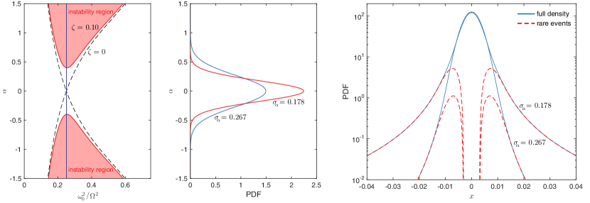
Figure 3: (Left) Stability diagram for constant (in time) $\alpha$ and for finite damping $\zeta=0.1$ (red shaded region); (Middle) pdf of the excitation $\alpha(t)$ for two different values of $\sigma_{\alpha}$; (Right) The corresponding analytical pdf of Mathieu’s equation according to the decomposition-sythesis method 44, where we have highlighted the conditionally rare event component (dashed red) in the full pdf (solid blue), showing that the tails are completely described by rare events, whereas the background dynamics fully determine the core (the response pdf is shown assuming $\ell_{\alpha}=10.0$, other parameters are described in section 6).

6 Comparisons with Monte-Carlo simulations

To illustrate the accuracy of our approximation 44, we compare the analytical formula obtained via the probabilistic-decomposition technique with direct Monte-Carlo simulations of the original system. To perform comparisons we use a unit white noise $\dot{W}(t)$ process with intensity $\nu$ for the additive forcing term $F(t)$, and furthermore non-dimensionalize time by $\omega_{0}$ in eq. 8 so that,

$$\ddot{x}(t)+2\zeta\dot{x}(t)+(1+\alpha(t)\sin 2t)x(t)=\nu\dot{W}(t).$$ (45)

Thus, for this additive forcing we have $\sigma_{F}^{2}=\nu^{2}/2\omega_{0}^{2}$.

To perform the Monte-Carlo simulations, we compute $3000$ realization of the above equation using the Euler-Maruyama method with time step $dt=5\times 10^{-3}$ from $t=0$ to $t=5500$ and discard the first $500$ time units, to ensure a statistical steady state. Moreover, we generate realizations of the stochastic process $\alpha(t)$ directly from the autocorrelation function by a statistically exact and efficient method using the circulant embedding technique [38].

In fig. 4 we show nine cases of varying intermittency levels. We fix the system parameters $\zeta=0.1$ and $\nu\ =0.002$. In the figure, we show the response pdf for three different correlation times $\ell_{\alpha}=2.5,\,5.0,\,10.0$ of and for three different values of the standard deviation of the parametric excitation $\alpha(t)$: $\sigma_{\alpha}=0.178,\,0.229,\,0.267$; For the least intermittent case the standard deviation of $\alpha(t)$ is $\sigma_{\alpha}=0.178$ so that rare event transitions occur with probability $\operatorname{\mathbb{P}}_{r}=0.0141$, for $\sigma_{\alpha}=0.229$ with probability $\operatorname{\mathbb{P}}_{r}=0.0488$, and for the most intermittent case $\operatorname{\mathbb{P}}_{r}=0.0847$.

Overall, the results presented, along with additional numerical comparisons, show good quantitative agreement for both the tails and the core of the distribution between our analytic formula in eq. 44 and the ‘true’ density from Monte-Carlo simulations; indeed, the quantitative agreement between our formula and the actual density is found to be robust across a range of parameters that satisfy the assumptions. We observe our result performs better with the averaged system, on which we directly derived the density, than the original system for cases with larger correlation times $\ell_{\alpha}$ and larger variance $\sigma_{\alpha}^{2}$ in the parametric excitation process $\alpha(t)$; this behavior is expected since averaging introduces well known errors that increase for more intermittent regimes, because the instabilities in such cases lead to even larger amplitude responses. Moreover, we observe that even in extremely intermittent regimes, where our assumptions start to be violated, namely the statistical independence of rare events, our analytical formula is still able to capture the asymptotic behavior of the tails.

Clearly, the results show that the response pdf is far from Gaussian, and highlight the non-Gaussianity of roll motions during parametric resonance. Despite the simplicity and theoretical nature of our model, the overall characteristics and shape of the distribution is the same as that observed in Monte-Carlo simulations using advanced hydrodynamic codes with three degrees of freedom that account for coupled pitch, heave, and roll motions [39, 40].

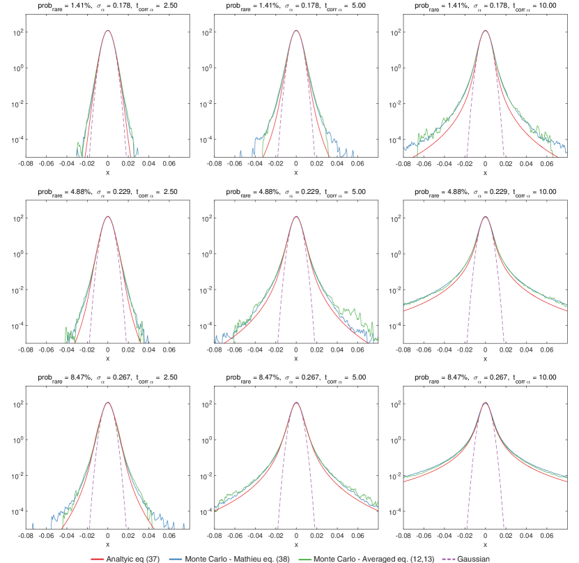
Figure 4: Comparisons of Monte-Carlo simulations (blue curve) of Mathieu’s eq. 45 the ‘true’ density, the averaged system eqs. 16 and 17 (green curve), and our analytical formula 44 (red curve), along with a Gaussian approximation (dashed purple curve), where the variance is obtained by a traditional averaging procedure. The left column corresponds to a parametric excitation process with correlation time-scale of $\ell_{\alpha}=2.5$, the middle column $\ell_{\alpha}=5.0$, and the right column $\ell_{\alpha}=10.0$; note the time scale of damping is $t_{\text{damp}}\sim 1/\zeta=10.0$. In the top row the excitation standard deviation is $\sigma_{\alpha}=0.148$, middle row $\sigma_{\alpha}=0.229$, and the bottom row $\sigma_{\alpha}=0.267$. Fixed system parameters: $\zeta=0.01$ and $\nu=0.002$.

7 Conclusions

In this work we derived an analytical approximation to the heavy-tailed stationary measure of Mathieu’s equation under parametric excitation by a correlated stochastic process in a regime undergoing intermittent parametric resonances. We derived the formula for the case when the spectrum of the noise is peaked at the main resonant frequency. To derive the pdf for the response we averaged the governing equation over the fast frequency to arrive at a set of parametrically excited processes that govern the slow dynamics. We then applied the probabilistic decomposition-synthesis method to the slow variables. We demonstrated the accuracy of the final formula for the pdf through direct comparisons with Monte-Carlo results for a range parameters that influence the rare event transition probability level and severity of the resonance phenomena; the analytical formula showed excellent quantitative agreement with results from numerical simulations across a wide range of intermittency levels. The approach is also directly applicable for the determination of the local maxima of the response.

The presented analysis paves the way for the analytical treatment of more realistic ship roll models. Future work includes the inclusion of nonlinear terms, in particular, softening nonlinearity in the restoring force, which would modify the statistical characteristics of the tails. Such a problem could be considered through the current framework by analytical modeling of the nonlinear terms during the rare transitions, in combination with appropriate nonlinear closures for the background stochastic attractor. Additional work will include application of the decomposition-synthesis method in a data-driven context using models containing model error to derive tail estimates.

References

- [1] W. Chai, A. Naess, B. J. Leira, Stochastic nonlinear ship rolling in random beam seas by the path integration method, Probabilistic Engineering Mechanics.
- [2] H. Lin, S. C. Yim, Chaotic roll motion and capsize of ships under periodic excitation with random noise, Applied Ocean Research 17 (3) (1995) 185–204.
- [3] I. A. Kougioumtzoglou, P. D. Spanos, Stochastic response analysis of the softening Duffing oscillator and ship capsizing probability determination via a numerical path integral approach, Probabilistic Engineering Mechanics 35 (2014) 67–74.
- [4] E. Kreuzer, W. Sichermann, The effect of sea irregularities on ship rolling, Computing in Science and Engineering May/June (2006) 26–34.
- [5] A. J. Majda, Y. Lee, Conceptual dynamical models for turbulence., Proceedings of the National Academy of Sciences of the United States of America 111 (18) (2014) 6548–53.
- [6] A. J. Majda, X. Tong, Intermittency in Turbulent Diffusion Models with a Mean Gradient, Nonlinearity 28 (11).
- [7] D. Qi, A. J. Majda, Predicting Fat-Tailed Intermittent Probability Distributions in Passive Scalar Turbulence with Imperfect Models through Empirical Information Theory, accepted Communications in Mathematical Sciences.
- [8] A. Abou-Rayan, A. Nayfeh, Stochastic response of a buckled beam to external and parametric random excitations, in: AIAA/ASME/ASCE/AHS/ASC 34th Structures, Structural Dynamics, and Materials Conference, Vol. 1, 1993, pp. 1030–1040.
- [9] Y. K. Lin, C. Q. Cai, Probabilistic structural dynamics : advanced theory and applications, New York: McGraw-Hill, 2004.
- [10] A. H. Nayfeh, D. T. Mook, Nonlinear Oscillations, Wiley-Interscience, New York, 1984.
- [11] V. L. Belenky, N. B. Sevastianov, Stability and Safety of Ships: Risk of Capsizing, Society of Naval Architects and Marine Engineers, Jersey City, NJ, 2007.
- [12] L. Arnold, I. Chueshov, G. Ochs, Stability and capsizing of ships in random sea - a survey, Nonlinear Dynamics 36 (2004) 135–179.
- [13] T. I. Fossen, H. Nijmeijer (Eds.), Parametric resonance in dynamical systems, Springer-Verlag New York, 2012.
- [14] J. R. Paulling, R. M. Rosenberg, On unstable ship motions resulting from nonlinear coupling, Journal of Ship Research 3 (1) (1959) 36 – 46.
- [15] J. Paulling, O. H. Oakley, P. Wood, Ship capsizing in heavy seas: the correlation of theory and experiments, in: Proceedings of the 1st International Conference on Stability of Ships and Ocean Vehicles, Glasgow, 1975.
- [16] W. France, M. Levadou, T. Treakle, J. Paulling, R. Michel, C. Moore, An investigation of head-sea parametric rolling and its influence on container lashing systems., Marine Technology and SNAME news 40 (1) (2003) 1 – 19.
- [17] American Bureau of Shipping, Guide for the assessment of parametric roll resonance in the design of container carriers (2004 - original publication, 2008 - amendment).
- [18] A. Francescutto, Intact stability of ships past present and future, in: Proceedings of the 12th International Conference on Stability of Ships and Ocean Vehicles, Glasgow, U.K., 2015, pp. 1199–1209.
- [19] M. A. Neves, C. A. Rodírguez, Influence of non-linearities on the limits of stability of ships rolling in head seas, Ocean Engineering 34 (11 - 12) (2007) 1618 – 1630.
- [20] P. A. D. Spyrou, K. J., Ship design for dynamic stability, in: Proceedings of the 7th International Marine Design Conference, Kyongju, Korea, 199, pp. 167–178.
- [21] A. Champneys, Dynamics of parametric excitation, in: R. A. Meyers (Ed.), Encyclopedia of Complexity and Systems Science, Springer New York, 2009, pp. 2323–2345.
- [22] T. Soong, M. Grigoriu, Random Vibration of Mechanical and Structural Systems, PTR Prentice Hall, 1993.
- [23] F. J. Poulin, G. R. Flierl, The stochastic mathieu’s equation, Proceedings of the Royal Society of London A: Mathematical, Physical and Engineering Sciences 464 (2095) (2008) 1885–1904.
- [24] F. C. Adams, A. M. Bloch, Hill’s equation with random forcing terms, SIAM Journal on Applied Mathematics 68 (4) (2008) 947–980.
- [25] R. L. Stratonovich, Topics in the theory of random noise. vol. 2., Mathematics and its applications, Gordon and Breach, New York, 1967.
- [26] M. A. Mohamad, T. P. Sapsis, Probabilistic description of extreme events in intermittently unstable dynamical systems excited by correlated stochastic processes, SIAM/ASA Journal on Uncertainty Quantification 3 (1) (2015) 709–736.
- [27] M. A. Mohamad, W. Cousins, T. P. Sapsis, A probabilistic decomposition-synthesis method for the quantification of rare events due to internal instabilities, Journal of Computational Physics 322 (2016) 288–308.
- [28] C. Soize, The Fokker-Planck equation for stochastic dynamical systems and its explicit steady state solutions, World Scientific, 1994.
- [29] A. J. Majda, M. Branicki, Lessons in uncertainty quantification for turbulent dynamical systems, Discrete and Continuous Dynamical Systems 32 (2012) 3133–3221.
- [30] A. Masud, L. A. Bergman, Solution of the four dimensional Fokker-Planck Equation: Still a challenge, ICOSSAR 2005 (2005) 1911–1916.
- [31] G. A. Pavliotis, A. Stuart, Multiscale Methods: Averaging and Homogenization, Springer Science & Business Media, 2008.
- [32] C. Floris, Stochastic stability of damped mathieu oscillator parametrically excited by a gaussian noise., Mathematical Problems in Engineering 2012 (2012) 1–18.
- [33] V. I. Klyatskin, Stochastic equations through the eye of the physicist, Elsevier Publishing Company, Amsterda, The Netherlands, 2005.
- [34] T. P. Sapsis, A. F. Vakakis, L. A. Bergman, Effect of stochasticity on targeted energy transfer from a linear medium to a strongly nonlinear attachment, Probabilistic Engineering Mechanics 26 (2011) 119–133.
- [35] S. O. Rice, Distribution of the duration of fades in radio transmission: Gaussian noise model, Bell System Tech. J. 37 (1958) 581–635.
- [36] I. F. Blake, W. C. Lindsey, Level-crossing problems for random processes, IEEE Trans. Information Theory IT-19 (1973) 295–315.
- [37] R. Langley, On various definitions of the envelope of a random process., Journal of Sound and Vibration 105 (3) (1986) 503 – 512.
- [38] D. P. Kroese, Z. I. Botev, Spatial process simulation, in: Stochastic Geometry, Spatial Statistics and Random Fields, Springer, 2015, pp. 369–404.
- [39] V. Belenky, K. M. Weems, W.-M. Lin, J. Paulling, Probabilistic analysis of roll parametric resonance in head seas, in: M. Almeida Santos Neves, V. L. Belenky, J. O. de Kat, K. Spyrou, N. Umeda (Eds.), Contemporary Ideas on Ship Stability and Capsizing in Waves, Vol. 97 of Fluid Mechanics and Its Applications, Springer Netherlands, 2011, pp. 555–569.
- [40] V. Belenky, K. M. Weems, Probabilistic properties of parametric roll, in: T. I. Fossen, H. Nijmeijer (Eds.), Parametric Resonance in Dynamical Systems, Springer New York, 2012, pp. 129–145.