Symmetrization and extension of planar bi-Lipschitz maps

Abstract.

We show that every centrally symmetric bi-Lipschitz embedding of the circle into the plane can be extended to a global bi-Lipschitz map of the plane with linear bounds on the distortion. This answers a question of Daneri and Pratelli in the special case of centrally symmetric maps. For general bi-Lipschitz embeddings our distortion bound has a combination of linear and cubic growth, which improves on the prior results. The proof involves a symmetrization result for bi-Lipschitz maps which may be of independent interest.

1. Introduction

A map $f\colon X\to Y$ between subsets of Euclidean spaces is called a bi-Lipschitz embedding if there exist positive constants $L$ and $\ell$ such that

(1.1) $$\ell\lvert a-b\rvert\leq\lvert f(a)-f(b)\rvert\leq L\lvert a-b\rvert,\quad a,b\in X.$$

To emphasize the role of constants, $f$ may be called $(L,\ell)$-bi-Lipschitz. The lower bound $\ell$ is often taken to be $1/L$ in the literature but for our purpose keeping track of two constants separately is more natural.

The Lipschitz Schoenflies theorem was proved by Tukia in [23, 24] (see also [14, 17]). It asserts that every bi-Lipschitz embedding $f\colon\mathbb{T}\to\mathbb{C}$, where $\mathbb{T}$ is the unit circle, can be extended to a global bi-Lipschitz map $F$. In its original form this theorem was not quantitative in that it did not provide Lipschitz constants $(L^{\prime},\ell^{\prime})$ for the extension.

Daneri and Pratelli [8] obtained a quantitative bi-Lipschitz extension theorem: an $(L,1/L)$-bi-Lipschitz embedding $f\colon\mathbb{T}\to\mathbb{C}$ has a $(CL^{4},1/(CL^{4}))$-bi-Lipschitz extension with a universal constant $C$. They asked whether linear control of the distortion constants is possible, which is a natural question considering that linear distortion bounds are standard for Lipschitz extension problems [7]. The following theorem provides such a result for the upper Lipschitz constant $L^{\prime}$, while the lower constant $\ell^{\prime}$ is cubic (which is still an improvement on the aforementioned $4$th degree estimate).

Theorem 1.1.

Every $(L,\ell)$-bi-Lipschitz embedding $f\colon\mathbb{T}\to\mathbb{C}$ can be extended to an $(L^{\prime},\ell^{\prime})$-bi-Lipschitz automorphism $F\colon\mathbb{C}\to\mathbb{C}$ with $L^{\prime}=10^{28}L$ and $\ell^{\prime}=10^{-25}\ell^{2}/L$.

If the distortion is measured by the ratio of upper and lower Lipschitz constants, then Theorem 1.1 provides a quadratic bound, namely $L^{\prime}/\ell^{\prime}\leq 10^{53}(L/\ell)^{2}$.

A map $f$ is centrally symmetric if $f(-z)=-f(z)$ for all $z$ in the domain of $f$. For such maps we can settle the problem completely.

Theorem 1.2.

A centrally symmetric $(L,\ell)$-bi-Lipschitz embedding $f\colon\mathbb{T}\to\mathbb{C}$ can be extended to a centrally symmetric $(L^{\prime},\ell^{\prime})$-bi-Lipschitz automorphism $F\colon\mathbb{C}\to\mathbb{C}$ with $L^{\prime}=10^{27}L$ and $\ell^{\prime}=10^{-23}\ell$.

Recent papers on quantitative bi-Lipschitz extension include [2, 3, 4, 5, 15, 16, 18, 22]. In particular, Alestalo and Väisälä [4] observed that the bi-Lipschitz form of the Klee trick incurs quadratic distortion growth; it is unclear whether this can be made linear. In [16] the author proved that bi-Lipschitz extension with linear distortion bounds is possible for maps $f\colon\mathbb{R}\to\mathbb{C}$. It should be noted that while conjugation by a Möbius map appears to reduce the extension problem for $\mathbb{T}$ to the same problem for $\mathbb{R}$, this is not so when linear distortion bounds are desired. Conjugating, extending, and conjugating back yields nonlinear bounds such as $CL^{9}$.

The paper is structured as follows. Section 2 relates harmonic measure to metric properties of sets, following the Beurling-Nevanlinna theorem. Section 3 uses harmonic measure to estimate the derivative of a conformal map that will be used in the extension process. In §4 we study the properties of an extension of a circle homeomorphism obtained by the Beurling-Ahlfors method [6]. It would be interesting to employ the conformally natural Douady-Earle extension [9] instead, but its nonlocal nature presents an obstacle.

In §5 the aforementioned results are combined to produce an extension of a centrally symmetric embedding of $\mathbb{T}$ to a bi-Lipschitz map of the unit disk $\mathbb{D}$. The exterior domain $\mathbb{C}\setminus\overline{\mathbb{D}}$ requires a separate treatment; as noted above, Möbius conjugation is not an option for us. The required estimates for harmonic measure and conformal maps of $\mathbb{C}\setminus\overline{\mathbb{D}}$ are obtained in §6, and this allows the proof of Theorem 1.2 to be completed in §7. To derive Theorem 1.1 from Theorem 1.2, we develop a symmetrization process for bi-Lipschitz maps in §8. The paper concludes with §9 presenting the proof of Theorem 1.1 and some open questions.

Throughout the paper, $D(a,r)$ is the open disk of radius $r$ with center $a$. As a special case, $\mathbb{D}=D(0,1)$ is the unit disk, and $\mathbb{T}=\partial\mathbb{D}$ is the unit circle.

2. Harmonic measure estimates

Our starting point is a classical harmonic measure estimate [21, Corollary 4.5.9] which is a consequence of the Beurling-Nevanlinna projection theorem.

Proposition 2.1.

Let $\Omega\subset\mathbb{C}\setminus\{0\}$ be a simply connected domain. Pick a point $\zeta\in\Omega$ and let $\rho>0$.

(a) If $\lvert\zeta\rvert<\rho$, then

(2.1) $$\omega(\zeta,\partial\Omega\cap D(0,\rho),\Omega)\geq\frac{2}{\pi}\sin^{-1}\left(\frac{\rho-\lvert\zeta\rvert}{\rho+\lvert\zeta\rvert}\right).$$

(b) If $\lvert\zeta\rvert>\rho$, then

(2.2) $$\omega(\zeta,\partial\Omega\cap\overline{D}(0,\rho),\Omega)\leq\frac{2}{\pi}\cos^{-1}\left(\frac{\lvert\zeta\rvert-\rho}{\lvert\zeta\rvert+\rho}\right).$$

We need the following corollary of Proposition 2.1.

Corollary 2.2.

Let $\Omega\subset\mathbb{C}$ be a simply connected domain. Consider a point $\zeta\in\Omega$ and a subset $\Gamma\subset\partial\Omega$. Suppose that $\omega(\zeta,\Gamma,\Omega)\geq\epsilon>0$. Then

(2.3) $$\operatorname{dist}(\zeta,\Gamma)\leq\csc^{2}\left(\frac{\pi\epsilon}{4}\right)\operatorname{dist}(\zeta,\partial\Omega);$$

(2.4) $$\operatorname{diam}\Gamma\geq\tan^{2}\left(\frac{\pi\epsilon}{4}\right)\operatorname{dist}(\zeta,\Gamma).$$

Proof.

To prove (2.3), translate $\Omega$ so that $0$ is a nearest boundary point to $\zeta$, that is $0\in\partial\Omega$ and $\operatorname{dist}(z,\Omega)=\lvert\zeta\rvert$. Let $\rho=\operatorname{dist}(\zeta,\Gamma)-\lvert\zeta\rvert$. If $\rho\leq\lvert\zeta\rvert$, then $\operatorname{dist}(\zeta,\Gamma)\leq 2\operatorname{dist}(z,\Omega)$ and so  (2.3) holds. Otherwise, (2.1) implies

(2.5) $$\frac{2}{\pi}\sin^{-1}\left(\frac{\rho-\lvert\zeta\rvert}{\rho+\lvert\zeta\rvert}\right)\leq\omega(\zeta,\partial\Omega\cap D(0,\rho),\Omega)\leq 1-\epsilon$$

where the second inequality holds because $D(0,\rho)$ is disjoint from $\Gamma$. Rearranging (2.5) yields $\rho/\lvert\zeta\rvert\leq\cot^{2}(\pi\epsilon/4)$, which implies  (2.3).

To prove (2.4), translate $\Omega$ so that $0\in\Gamma$. Let $\rho=\operatorname{diam}\Gamma$ and note that $\Gamma\subset\overline{D}(0,\rho)$. If $\lvert\zeta\rvert\leq\rho$, then $\operatorname{dist}(\zeta,\Gamma)\leq\operatorname{diam}\Gamma$ and so (2.4) holds. Otherwise, by (2.2),

$$\frac{2}{\pi}\cos^{-1}\left(\frac{\lvert\zeta\rvert-\rho}{\lvert\zeta\rvert+\rho}\right)\geq\omega(\zeta,\partial\Omega\cap D(0,\rho),\Omega)\geq\epsilon$$

which implies $\lvert\zeta\rvert/\rho\leq\cot^{2}(\pi\epsilon/4)$, i.e., (2.4). ∎

Given a point $z=re^{i\theta}$ with $e^{-2\pi}<r<1$, let $\delta=\log(1/r)$ and introduce four arcs of the unit circle $\mathbb{T}$:

(2.6) $$\begin{split}&\gamma_{1}=\{e^{it}\colon\theta-2\delta\leq t\leq\theta-\delta\}\\ &\gamma_{2}=\{e^{it}\colon\theta-\delta\leq t\leq\theta-\delta/2\}\\ &\gamma_{3}=\{e^{it}\colon\theta+\delta/2\leq t\leq\theta+\delta\}\\ &\gamma_{4}=\{e^{it}\colon\theta+\delta\leq t\leq\theta+2\delta\}\end{split}$$

Since the length of each arc is comparable to its distance from $z$, one expects its harmonic measure with respect to $z$ to be bounded below by a positive constant. The following lemma makes this explicit. The constraints on $\lvert z\rvert$ in (2.7) and  (2.8) are imposed so that the arcs involved are contained in a semicircle, which will be important later.

Lemma 2.3.

Using notation (2.6) for $j=1,\dots,4$, we have

(2.7) $$\omega(z,\gamma_{j},\mathbb{D})\geq\frac{1}{30\pi}\quad\text{if $j=1,4$ and $e^{-\pi/4}<|z|<1$}$$

and

(2.8) $$\omega(z,\gamma_{j},\mathbb{D})\geq\frac{1}{64\pi}\quad\text{if $j=2,3$ and $e^{-2\pi}<|z|<1$}$$

Proof.

Since the logarithmic function is concave, the function $x\mapsto\log x/(x-1)$ is decreasing for $x>1$. Therefore,

(2.9) $$1<\frac{\log(1/r)}{1-r}<\frac{\pi/4}{1-e^{-\pi/4}}<2\quad\text{for }\ e^{-\pi/4}<r<1.$$

and

(2.10) $$1<\frac{\log(1/r)}{1-r}<\frac{2\pi}{1-e^{-2\pi}}<7\quad\text{for }\ e^{-2\pi}<r<1.$$

For $\zeta\in\gamma_{j}$, $j=1,4$, the triangle inequality and  (2.9) imply

$$\lvert\zeta-z\rvert^{2}\leq|1-r+2\delta||1-r+2\delta|<5(1-r)(3\delta)=15(1-r)\delta$$

This leads to Poisson kernel estimates, using the explicit form of the kernel [12, Theorem I.1.3]:

$$P_{z}(\zeta)=\frac{1}{2\pi}\frac{1-r^{2}}{\lvert\zeta-z\rvert^{2}}\geq\frac{1}{2\pi}\frac{1-r}{15(1-r)\delta}=\frac{1}{30\pi\delta}$$

Since the length of $\gamma_{j}$ is $\delta$, inequality (2.7) follows.

Similarly, for $j=2,3$ we use (2.10) to obtain

$$\lvert\zeta-z\rvert^{2}\leq|1-r+\delta||1-r+\delta|<8(1-r)(2\delta)=16(1-r)\delta$$

hence $P_{z}(\zeta)\geq 1/(32\pi\delta)$. Since the length of $\gamma_{j}$ is $\delta/2$, inequality (2.8) follows. ∎

3. Conformal map onto a Jordan domain

The harmonic measure estimates in §2 allow us to control the derivative of a conformal map in terms of the images of boundary arcs $\gamma_{j}$ introduced in (2.6).

Lemma 3.1.

Let $\Omega\subsetneq\mathbb{C}$ be a Jordan domain. Fix a conformal map $\Phi$ of $\mathbb{D}$ onto $\Omega$ and consider a point $z=re^{i\theta}$ with $e^{-2\pi}<r<1$. Referring to notation (2.6), let $\Gamma_{j}\subset\partial\Omega$ be the image of $\gamma_{j}$ under the boundary map induced by $\Phi$. Also let $\zeta=\Phi(z)$ and $\rho=\operatorname{dist}(\zeta,\partial\Omega)$. Then

(3.1) $$\lvert\Phi^{\prime}(z)\rvert\geq\frac{\operatorname{dist}(\Gamma_{1},\Gamma_{4})}{60000\log(1/r)},\quad e^{-\pi/4}<r<1,$$

and

(3.2) $$\lvert\Phi^{\prime}(z)\rvert\leq 2\cdot 10^{6}\,\dfrac{\min(\operatorname{diam}\Gamma_{2},\operatorname{diam}\Gamma_{3})}{\log(1/r)},\quad e^{-2\pi}<r<1.$$

Proof.

The Koebe $1/4$ theorem and the Schwarz lemma imply the standard estimate [20, Corollary 1.4]

(3.3) $$\rho\leq(1-r^{2})|\Phi^{\prime}(z)|\leq 4\rho.$$

A concavity argument similar to (2.9)–(2.10) yields

(3.4) $$\frac{1}{2}<\frac{\log(1/r)}{1-r^{2}}<\frac{\pi/4}{1-e^{-\pi/2}}<1\quad\text{for }\ e^{-\pi/4}<r<1,$$

and

(3.5) $$\frac{1}{2}<\frac{\log(1/r)}{1-r^{2}}<\frac{2\pi}{1-e^{-4\pi}}<7\quad\text{for }\ e^{-2\pi}<r<1.$$

Proof of  (3.1) for $e^{-\pi/4}<r<1$. From  (2.3) and  (2.7) it follows that

$$\operatorname{dist}(\Gamma_{1},\Gamma_{4})\leq\operatorname{dist}(\zeta,\Gamma_{1})+\operatorname{dist}(\zeta,\Gamma_{4})\leq 2\csc^{2}\left(\frac{1}{120}\right)\rho\leq 30000\rho$$

which in view of (3.3) and (3.4) implies

$$\lvert\Phi^{\prime}(z)\rvert\geq\frac{\rho}{1-r^{2}}\geq\frac{\operatorname{dist}(\Gamma_{1},\Gamma_{4})}{30000(1-r^{2})}\geq\frac{\operatorname{dist}(\Gamma_{1},\Gamma_{4})}{60000\log(1/r)}$$

proving (3.1).

Proof of  (3.2) for $e^{-2\pi}<r<1$. From  (2.4) and  (2.8) it follows that

$$\min(\operatorname{diam}\Gamma_{2},\operatorname{diam}\Gamma_{3})\geq\tan^{2}\left(\frac{1}{256}\right)\rho$$

hence

$$\lvert\Phi^{\prime}(z)\rvert\leq\frac{4\rho}{1-r^{2}}\leq\frac{4\min(\operatorname{diam}\Gamma_{2},\operatorname{diam}\Gamma_{3})}{\tan^{2}\left(\frac{1}{256}\right)(1-r^{2})}<2\cdot 10^{6}\frac{\min(\operatorname{diam}\Gamma_{2},\operatorname{diam}\Gamma_{3})}{\log(1/r)}$$

where the last step uses  (3.5). ∎

4. Extension of a circle homeomorphism

A key element of the proof, going back to Tukia [24], is pre-composing a conformal map with a disk homeomorphism obtained by extending a suitable circle homeomorphism. This extension is carried out below. Lemma 4.1 is where the assumption of central symmetry is crucial: it ensures that the image of any set contained in a semicircle is also contained in a semicircle, enabling the comparison of intrinsic and extrinsic distances on $\mathbb{T}$.

A sense-preserving circle homeomorphism $\psi\colon\mathbb{T}\to\mathbb{T}$ lifts to an increasing homeomorphism $\chi$ of the real line onto itself, which satisfies $\psi(e^{it})=e^{i\chi(t)}$ for all $t\in\mathbb{R}$, and $\chi(t+2\pi)=\chi(t)+2\pi$. As a consequence,

(4.1) $$\lvert\chi(t)-t-\chi(0)\rvert\leq 2\pi,\quad t\in\mathbb{R}.$$

Let $\chi_{e}$ denote the following variant of the Beurling-Ahlfors extension of $\chi$:

(4.2) $$\chi_{e}(x+iy)=\frac{1}{2}\int_{-1}^{1}\chi(x+ty)(1+2i\operatorname{sign}t)\,dt.$$

This is a diffeomorphism of the upper halfplane onto itself [1, 6]. It differs from the map considered in  [1] only by the factor of $2$ in front of the imaginary part. The contribution of this factor is that the derivative matrix $D\chi_{e}$ is multiplied by $\left(\begin{smallmatrix}1&0\\ 0&2\end{smallmatrix}\right)$ on the left. Due to the submultiplicativity of operator norm, the inequalities (4.9) and (4.11) from [16] still apply to this variant of the extension, with an extra factor of $2$:

(4.3) $$\lVert D\chi_{e}(x+iy)\rVert\leq 2\,\frac{\chi(x+y)-\chi(x-y)}{y}$$

(4.4) $$\lVert D\chi_{e}(x+iy)^{-1}\rVert\leq\frac{4y}{\min(\chi(x+y)-\chi(x+\frac{y}{2}),\chi(x-\frac{y}{2})-\chi(x-y))}$$

The reason for inserting $2$ in front of $i\operatorname{sign}t$ in (4.2) is the following estimate, which employs (4.1); it asserts that $\chi_{e}$ maps each horizontal line onto a curve with a bounded distance from the line.

(4.5) $$\begin{split}\lvert\operatorname{Im}\chi_{e}(x+iy)-y\rvert&=\left|\int_{-1}^{1}(\chi(x+ty)-ty)\operatorname{sign}t\,dt\right|\\ &=\left|\int_{-1}^{1}(\chi(x+ty)-(x+ty+\chi(0)))\operatorname{sign}t\,dt\right|\\ &\leq 4\pi\end{split}$$

Since $\chi$ commutes with translation by $2\pi$, so does $\chi_{e}$: that is, $\chi_{e}(z+2\pi)=\chi_{e}(z)+2\pi$. This allows us to define a map $\Psi$ of the unit disk $\mathbb{D}$ onto itself as follows.

(4.6) $$\Psi(e^{iz})=\exp(i\chi_{e}(z)),\quad\Psi(0)=0$$

This is a diffeomorphism of the punctured disk $\mathbb{D}\setminus\{0\}$ onto itself, and also a homeomorphism of $\mathbb{D}$ onto $\mathbb{D}$. According to (4.5),

(4.7) $$e^{-4\pi}\lvert\zeta\rvert\leq\lvert\Psi(\zeta)\rvert\leq e^{4\pi}\lvert\zeta\rvert,\quad\zeta\in\mathbb{D}.$$

Using the chain rule and (4.7), we obtain

(4.8) $$\lVert D\Psi(e^{iz})\rVert\leq e^{4\pi}\lVert D\chi_{e}(z)\rVert,\qquad\lVert D\Psi(e^{iz})^{-1}\rVert\leq e^{4\pi}\lVert D\chi_{e}(z)^{-1}\rVert.$$

Lemma 4.1.

Let $\psi\colon\mathbb{T}\to\mathbb{T}$ be a sense-preserving circle homeomorphism such that

(4.9) $$\psi(-z)=-\psi(z),\quad z\in\mathbb{T}$$

Let $\Psi\colon\mathbb{D}\to\mathbb{D}$ be the extension of $\psi$ defined by (4.6). Fix a point $z=re^{i\theta}$ with $0<r<1$. Referring to notation (2.6), let $\sigma_{j}\subset\mathbb{T}$ be the image of $\gamma_{j}$ under $\psi$. Then the derivative matrix $D\Psi(z)$ satisfies

(4.10) $$\lVert D\Psi(z)\rVert\leq\begin{cases}e^{4\pi}\pi\dfrac{\operatorname{dist}(\sigma_{1},\sigma_{4})}{\log(1/r)},\quad&e^{-\pi/4}<r<1;\\ 20e^{4\pi},\quad&0<r\leq e^{-\pi/4}\end{cases}$$

and

(4.11) $$\lVert D\Psi(z)^{-1}\rVert\leq\begin{cases}\dfrac{4e^{4\pi}\log(1/r)}{\min(\operatorname{diam}\sigma_{2},\operatorname{diam}\sigma_{3})},\quad&e^{-2\pi}<r<1;\\ 16e^{4\pi},\quad&0<r\leq e^{-2\pi};\end{cases}$$

Proof.

Note that $\Psi(re^{i\theta})=\exp(i\chi_{e}(\theta+i\delta))$ where $\delta=\log(1/r)$. The central symmetry property  (4.9) implies that the lifted homeomorphism $\chi\colon\mathbb{R}\to\mathbb{R}$ satisfies

(4.12) $$\chi(t+\pi)=\chi(t)+\pi$$

and the same holds for its extension $\chi_{e}$. Consequently, $\Psi$ inherits the central symmetry.

Proof of (4.10). In view of (4.8), the estimate  (4.3) yields

(4.13) $$\lVert D\Psi(z)\rVert\leq 2e^{4\pi}\,\frac{\chi(\theta+\delta)-\chi(\theta-\delta)}{\delta}.$$

Suppose $r>e^{-\pi/4}$. Then the union $\gamma_{1}\cup\gamma_{4}$ is contained in a semicircle. Since $\psi$ is centrally symmetric, it maps a semicircle to another semicircle. Within a semicircle, Euclidean distance is comparable to arcwise distance. Specifically,

(4.14) $$\operatorname{dist}(\sigma_{1},\sigma_{4})\geq\frac{2}{\pi}(\chi(\theta+\delta)-\chi(\theta-\delta)).$$

From  (4.13) and (4.14), the inequality (4.10) follows.

Now consider the case $0<r\leq e^{-\pi/4}$. By virtue of  (4.12),

$$\chi(\theta+\delta)-\chi(\theta-\delta)\leq\pi\left(\left\lfloor\frac{2\delta}{\pi}\right\rfloor+2\right).$$

Since $2\leq 8\delta/\pi$, it follows that

$$\chi(\theta+\delta)-\chi(\theta-\delta)\leq\pi\left(\frac{2\delta}{\pi}+\frac{8\delta}{\pi}\right)=10\delta.$$

Returning to (4.13), we get $\lVert D\Psi(z)\rVert\leq 20e^{4\pi}$ in this case.

Proof of (4.11). In view of (4.8), the estimate  (4.4) yields

(4.15) $$\lVert D\Psi(z)^{-1}\rVert\leq\frac{4e^{4\pi}\delta}{\min(\chi(\theta+\delta)-\chi(\theta+\delta/2),\chi(\theta-\delta/2)-\chi(\theta-\delta))}.$$

First suppose $r>e^{-2\pi}$. The denominator of  (4.15) is the length of the shorter of the arcs $\sigma_{2},\sigma_{3}$. Hence it is bounded from below by the minimum of $\operatorname{diam}\sigma_{2}$ and $\operatorname{diam}\sigma_{3}$, which yields  (4.11).

Now consider the case $0<r\leq e^{-2\pi}$. Then $\delta/2\geq\pi$, which by  (4.12) implies

$$\chi(\theta+\delta)-\chi(\theta+\delta/2)\geq\pi\left\lfloor\frac{\delta/2}{\pi}\right\rfloor\geq\frac{\delta}{4}.$$

The same bound holds for $\chi(\theta-\delta/2)-\chi(\theta-\delta)$, which shows that the right hand side of  (4.15) is bounded above by $16e^{4\pi}$ and thus completes the proof of  (4.11). ∎

5. Bi-Lipschitz extension in the unit disk

In this section we prove a half of Theorem 1.2, constructing an extension of $f$ in the unit disk $\mathbb{D}$.

Theorem 5.1.

Any centrally symmetric $(L,\ell)$-bi-Lipschitz embedding $f\colon\mathbb{T}\to\mathbb{C}$ can be extended to a centrally symmetric embedding $F\colon\overline{\mathbb{D}}\to\mathbb{C}$ such that $F$ is differentiable in $\mathbb{D}\setminus\{0\}$ and its derivative matrix $DF$ satisfies $\lVert DF\rVert\leq 10^{13}L$ and $\lVert DF^{-1}\rVert\leq 10^{11}/\ell$ in $\mathbb{D}\setminus\{0\}$.

Proof.

There is no loss of generality in assuming $f$ is sense-preserving; that is, the Jordan curve $f(\mathbb{T})$ is traversed counter-clockwise. This curve divides the plane in two domains, one of which, denoted $\Omega$, is bounded and contains $0$. Note that

(5.1) $$B(0,\ell)\subset\Omega\subset B(0,L)$$

because the quantity

$$\lvert f(z)\rvert=\frac{\lvert f(z)-f(-z)\rvert}{\lvert z-(-z)\rvert},\quad z\in\mathbb{T}$$

is bounded between $\ell$ and $L$.

Let $\Phi$ a conformal map of $\mathbb{D}$ onto $\Omega$ such that $\Phi(0)=0$. Note that $\Phi(-z)=-\Phi(z)$ by the uniqueness of such a map (up to rotation of the domain $\mathbb{D}$). The inclusion (5.1) implies $\ell\leq\lvert\Phi^{\prime}(0)\rvert\leq L$ by the Schwarz lemma. The distortion theorem [10, Theorem 2.5] states that

(5.2) $$\ell\,\frac{1-\lvert z\rvert}{(1+\lvert z\rvert)^{3}}\leq\lvert\Phi^{\prime}(z)\rvert\leq L\,\frac{1+\lvert z\rvert}{(1-\lvert z\rvert)^{3}},\quad z\in\mathbb{D}.$$

By Carathéodory’s theorem, $\Phi$ extends to a homeomorphism between $\overline{\mathbb{D}}$ and $\overline{\Omega}$. Let $\phi\colon\mathbb{T}\to\partial\Omega$ be the induced boundary map.

Define $\psi\colon\mathbb{T}\to\mathbb{T}$ by $\psi=f^{-1}\circ\phi$. This is a sense-preserving circle homeomorphism, which is centrally symmetric because $f$ and $\phi$ are. Lemma 4.1 provides its extension $\Psi$ to the unit disk. For $e^{-\pi/4}<\lvert z\rvert<1$, the estimates (3.1) and  (4.10) yield

(5.3) $$\lVert D\Psi(z)\rVert\leq 60000e^{4\pi}\pi\frac{\operatorname{dist}(\sigma_{1},\sigma_{4})}{\operatorname{dist}(\Gamma_{1},\Gamma_{4})}\lvert\Phi^{\prime}(z)\rvert.$$

Note that $\Gamma_{j}=f(\sigma_{j})$ for $j=1,\dots,4$ because $f=\phi\circ\psi^{-1}$. The bi-Lipschitz property of $f$ will be used here in the form

(5.4) $$\operatorname{diam}\Gamma_{j}\leq L\operatorname{diam}\sigma_{j}\quad\text{and}\quad\operatorname{dist}(\Gamma_{j},\Gamma_{k})\geq\ell\operatorname{dist}(\sigma_{j},\sigma_{k}).$$

Hence (5.3) simplifies to

(5.5) $$\lVert D\Psi(z)\rVert\leq 60000e^{4\pi}\pi\ell^{-1}\lvert\Phi^{\prime}(z)\rvert\leq 10^{11}\ell^{-1}\lvert\Phi^{\prime}(z)\rvert.$$

For $0<\lvert z\rvert\leq e^{-\pi/4}$, we combine (4.10) and  (5.2) to obtain

(5.6) $$\lVert D\Psi(z)\rVert\leq 20e^{4\pi}\frac{(1+e^{-\pi/4})^{3}}{1-e^{-\pi/4}}\ell^{-1}\lvert\Phi^{\prime}(z)\rvert\leq 10^{11}\ell^{-1}\lvert\Phi^{\prime}(z)\rvert.$$

The composition $F=\Phi\circ\Psi^{-1}$ extends $f=\phi\circ\psi^{-1}$. By (5.5),  (5.6) and the chain rule, $\lVert DF^{-1}\rVert\leq 10^{11}/\ell$ in $\mathbb{D}\setminus\{0\}$.

For $e^{-2\pi}<\lvert z\rvert<1$ we use  (3.2) and  (4.11) to obtain

$$\lVert D\Psi(z)^{-1}\rVert\leq 8e^{4\pi}\cdot 10^{6}\,\frac{\min(\operatorname{diam}\Gamma_{2},\operatorname{diam}\Gamma_{3})}{\min(\operatorname{diam}\sigma_{2},\operatorname{diam}\sigma_{3})}\lvert\Phi^{\prime}(z)\rvert^{-1}\leq 10^{13}L\lvert\Phi^{\prime}(z)\rvert^{-1}$$

hence $\lVert DF\rVert\leq 10^{13}L$. When $0<\lvert z\rvert<e^{-2\pi}$ use  (4.11) and  (5.2) instead:

$$\lVert D\Psi(z)^{-1}\rVert\leq 16e^{4\pi}\frac{1+e^{-2\pi}}{(1-e^{-2\pi})^{3}}L\lvert\Phi^{\prime}(z)\rvert^{-1}$$

leading to the same conclusion $\lVert DF\rVert\leq 10^{13}L$. ∎

6. Harmonic measure and conformal mapping of an exterior domain

In this section $\Omega\subset\mathbb{C}$ is a domain such that $\mathbb{C}\setminus\Omega$ is compact, connected, and contains more than one point. Our goal is to obtain harmonic measure estimates similar to Corollary 2.2 and use them to prove an analog of Lemma 3.1. This will be done by applying a suitably chosen Möbius transformation that maps $\Omega$ onto a simply connected domain in $\mathbb{C}$ minus one point (the image of $\infty$). Since removing one point does not change the harmonic measure, it can be ignored.

Lemma 6.1.

Let $\Omega\subset\mathbb{C}$ be a domain with compact connected complement containing more than one point. Let $K=\partial\Omega$ and consider a point $\zeta\in\Omega$ and a subset $\Gamma\subset K$ such that $\omega(\zeta,\Gamma,\Omega)\geq\epsilon>0$. Then

(6.1) $$\operatorname{dist}(\zeta,\Gamma)\leq 4\csc^{2}\left(\frac{\pi\epsilon}{4}\right)\operatorname{dist}(\zeta,K);$$

(6.2) $$\operatorname{diam}\Gamma\geq\frac{1}{4}\tan^{2}\left(\frac{\pi\epsilon}{4}\right)\frac{(\operatorname{diam}K-\operatorname{diam}\Gamma)^{2}}{\operatorname{diam}K(\operatorname{diam}K+\operatorname{dist}(\zeta,\Gamma))}\operatorname{dist}(\zeta,\Gamma).$$

Proof.

In order to prove (6.1), translate $K$ so that $0\in K$ and $0$ is the point of $K$ that is furthest from $\zeta$. Let $z_{1}$ be a point of $K$ that is closest to $\zeta$. If $\lvert\zeta\rvert<2\lvert z_{1}-\zeta\rvert$, then (6.1) holds in the stronger form $\operatorname{dist}(\zeta,\Gamma)<2\operatorname{dist}(\zeta,K)$. So we may assume $\lvert\zeta\rvert\geq 2\lvert z_{1}-\zeta\rvert$, hence $\lvert z_{1}\rvert\geq\lvert\zeta\rvert/2$.

Under the Möbius transformation $z\mapsto 1/z$ the sets $\Gamma$ and $K$ are mapped onto sets $\tilde{\Gamma}$ and $\tilde{K}$, with the latter certain to be unbounded. Since the harmonic measure is invariant under this transformation, Corollary 2.2 yields

(6.3) $$\operatorname{dist}(1/\zeta,\tilde{\Gamma})\leq\csc^{2}\left(\frac{\pi\epsilon}{4}\right)\operatorname{dist}(1/\zeta,\tilde{K}).$$

Using the point $z_{1}\in K$ chosen above, we get

(6.4) $$\operatorname{dist}(1/\zeta,\tilde{K})\leq\lvert 1/\zeta-1/z_{1}\rvert=\frac{\lvert\zeta-z_{1}\rvert}{\lvert\zeta\rvert\lvert z_{1}\rvert}\leq\frac{2\operatorname{dist}(\zeta,K)}{\lvert\zeta\rvert^{2}}.$$

Let $w\in\tilde{\Gamma}$ be a point realizing the distance $\operatorname{dist}(1/\zeta,\tilde{\Gamma})$. Since $1/w\in K$ and $0$ is the furthest point of $K$ from $\zeta$, it follows that $\lvert 1/w\rvert\leq 2\lvert\zeta\rvert$. Hence

(6.5) $$\operatorname{dist}(\zeta,\Gamma)\leq\lvert\zeta-1/w\rvert=\frac{\lvert w-1/\zeta\rvert\lvert\zeta\rvert}{\lvert w\rvert}\leq 2\lvert\zeta\rvert^{2}\operatorname{dist}(1/\zeta,\tilde{\Gamma}).$$

Combining (6.3)–(6.5) yields (6.1).

Proof of (6.2). If $\operatorname{diam}\Gamma=\operatorname{diam}K$ there is nothing to prove. Otherwise, let $\delta=(\operatorname{diam}K-\operatorname{diam}\Gamma)/2$ and observe that there exists a point $z_{1}\in K$ such that $\operatorname{dist}(z_{1},\Gamma)\geq\delta$. Translate $K$ so that $z_{1}=0$.

Under the transformation $z\mapsto 1/z$ the sets $\Gamma$ and $K$ are mapped onto sets $\tilde{\Gamma}$ and $\tilde{K}$, where $\tilde{K}$ is unbounded. By Corollary 2.2,

(6.6) $$\operatorname{diam}\tilde{\Gamma}\geq\tan^{2}\left(\frac{\pi\epsilon}{4}\right)\operatorname{dist}(1/\zeta,\tilde{\Gamma}).$$

Here

(6.7) $$\operatorname{diam}\tilde{\Gamma}=\sup_{a,b\in\Gamma}\frac{\lvert a-b\rvert}{\lvert a\rvert\lvert b\rvert}\leq\frac{\operatorname{diam}\Gamma}{\delta^{2}}.$$

Also,

(6.8) $$\operatorname{dist}(1/\zeta,\tilde{\Gamma})=\inf_{z\in\Gamma}\frac{\lvert z-\zeta\rvert}{\lvert z\rvert\lvert\zeta\rvert}\geq\frac{\operatorname{dist}(\zeta,\Gamma)}{\operatorname{diam}K(\operatorname{diam}K+\operatorname{dist}(\zeta,\Gamma))}$$

because $\lvert z\rvert\leq\operatorname{diam}K$. Combining (6.6)–(6.8) yields (6.2). ∎

Since the inequality (6.2) is more involved than its counterpart (2.4), we need an additional estimate in order to use it effectively.

Corollary 6.2.

Under the assumptions of Lemma 6.1, let $\Phi\colon\mathbb{C}\setminus\overline{\mathbb{D}}\to\Omega$ be a conformal map and let $z\in\mathbb{C}\setminus\overline{\mathbb{D}}$ be the point such that $\Phi(z)=\zeta$. Then

(6.9) $$\operatorname{diam}\Gamma\geq\frac{1}{32\lvert z\rvert}\tan^{2}\left(\frac{\pi\epsilon}{4}\right)\operatorname{dist}(\zeta,\Gamma).$$

Proof.

First observe that

(6.10) $$\operatorname{dist}(\zeta,\Gamma)\leq\lvert z\rvert\operatorname{diam}K.$$

Indeed, for any $w_{0}\in\Gamma$ the function $f(w)=(w-w_{0})/\Phi^{-1}(w)$ is holomorphic in $\Omega$, bounded at infinity, and bounded by $\operatorname{diam}K$ on the boundary of $\Omega$. Hence $\lvert f(w)\rvert\leq\operatorname{diam}K$, which yields (6.10) by letting $w=\zeta$.

If $\operatorname{diam}\Gamma>\frac{1}{2}\operatorname{diam}K$, then (6.9) holds by virtue of (6.10). It remains to consider the case $\operatorname{diam}\Gamma\leq\frac{1}{2}\operatorname{diam}K$. Since

$$\frac{(\operatorname{diam}K-\operatorname{diam}\Gamma)^{2}}{\operatorname{diam}K(\operatorname{diam}K+\operatorname{dist}(\zeta,\Gamma))}\geq\frac{(\operatorname{diam}K)^{2}/4}{\operatorname{diam}K(\operatorname{diam}K+\lvert z\rvert\operatorname{diam}K)}\geq\frac{1}{8\lvert z\rvert}$$

the estimate (6.2) simplifies to (6.9). ∎

Given a point $z=Re^{i\theta}$ with $1<R<e^{2\pi}$, let $\delta=\log R$ and introduce four arcs $\gamma_{1},\dots,\gamma_{4}\subset\mathbb{T}$ as in (2.6). The conformal invariance of harmonic measure yields an analog of Lemma 2.3 for this situation:

(6.11) $$\omega(z,\gamma_{j},\mathbb{C}\setminus\overline{\mathbb{D}})\geq\frac{1}{30\pi}\quad\text{if $j=1,4$ and $1<|z|<e^{\pi/4}$},$$

(6.12) $$\omega(z,\gamma_{j},\mathbb{C}\setminus\overline{\mathbb{D}})\geq\frac{1}{64\pi}\quad\text{if $j=2,3$ and $1<|z|<e^{2\pi}$}.$$

We proceed to the main result of the section: distortion estimates for a conformal map of $\mathbb{C}\setminus\overline{\mathbb{D}}$.

Lemma 6.3.

Let $\Omega\subset\mathbb{C}$ is a domain with compact connected boundary $K=\partial\Omega$. Fix a conformal map $\Phi$ of $\mathbb{C}\setminus\overline{\mathbb{D}}$ onto $\Omega$ and consider a point $z=Re^{i\theta}$ with $R>1$. Referring to notation (2.6), let $\Gamma_{j}\subset K$ be the image of $\gamma_{j}$ under the boundary map induced by $\Phi$. Also let $\zeta=\Phi(z)$. Then

(6.13) $$\lvert\Phi^{\prime}(z)\rvert\geq\begin{cases}\dfrac{\operatorname{dist}(\Gamma_{1},\Gamma_{4})}{600000\log R},\quad&1<R<e^{\pi/4};\\ (\operatorname{diam}K)/6,\quad&R\geq e^{\pi/4}\end{cases}$$

and

(6.14) $$\lvert\Phi^{\prime}(z)\rvert\leq\begin{cases}5\cdot 10^{9}\,\dfrac{\min(\operatorname{diam}\Gamma_{2},\operatorname{diam}\Gamma_{3})}{\log R},\quad&1<R<e^{2\pi};\\ \operatorname{diam}K,\quad&R\geq e^{2\pi}.\end{cases}$$

Proof.

The conformal map $\Phi$ has the asymptotic behavior $\Phi(z)=c/z+O(1)$ as $z\to\infty$, where $|c|$ is the logarithmic capacity of $K$, denoted $\operatorname{cap}K$. For a compact connected set $K$, the logarithmic capacity is comparable to diameter:

(6.15) $$2\operatorname{cap}K\leq\operatorname{diam}K\leq 4\operatorname{cap}K,$$

see [19, §11.1]. A distortion theorem due to Loewner (see section IV.3 in [13] or Corollary 3.3 in [19]) states that a univalent function $F\colon\mathbb{C}\setminus\overline{\mathbb{D}}\to\mathbb{C}$, normalized by $F(z)/z\to 1$ as $z\to\infty$, satisfies

(6.16) $$1-\frac{1}{\lvert z\rvert^{2}}\leq\lvert F^{\prime}(z)\rvert\leq\frac{1}{1-1/\lvert z\rvert^{2}}.$$

Combining (6.15) with (6.16) yields

$$\frac{1}{4}\operatorname{diam}K\left(1-\frac{1}{\lvert z\rvert^{2}}\right)\leq\lvert\Phi^{\prime}(z)\rvert\leq\frac{1}{2}\frac{\operatorname{diam}K}{1-1/\lvert z\rvert^{2}}$$

which takes care of the second half of (6.13) and (6.14).

Our next step is to prove the following distortion bounds, where $R=\lvert z\rvert$ and $\rho=\operatorname{dist}(\Phi(z),K)$:

(6.17) $$\lvert\Phi^{\prime}(z)\rvert\geq\frac{\rho}{5\log R},\quad 1<R<e^{\pi/4};$$

(6.18) $$\lvert\Phi^{\prime}(z)\rvert\leq\frac{4\rho}{\log R},\quad R>1.$$

Indeed, $(R^{2}-1)\lvert\Phi^{\prime}(z)\rvert\geq\rho$ is a consequence of the Schwarz-Pick lemma applied to $1/\Phi^{-1}$ in the disk $D(\Phi(z),\rho)$. The function $\log R/(R^{2}-1)$ is decreasing on the interval $(1,e^{\pi/4})$, hence is bounded below by its value at $e^{\pi/4}$, which is greater than $1/5$. The inequality (6.17) follows. To prove (6.18), apply the Koebe $1/4$ theorem to $\Phi$ in the disk $D(z,R-1)$. It yields $4\rho\geq(R-1)\lvert\Phi^{\prime}(z)\rvert\geq(\log R)\lvert\Phi^{\prime}(z)\rvert$ as claimed.

Proof of  (6.13) for $1<R<e^{\pi/4}$. From  (6.1) and  (6.11) it follows that

$$\operatorname{dist}(\Gamma_{1},\Gamma_{4})\leq\operatorname{dist}(\zeta,\Gamma_{1})+\operatorname{dist}(\zeta,\Gamma_{4})\leq 8\csc^{2}\left(\frac{1}{120}\right)\rho\leq 120000\rho$$

which in view of (6.17) implies

$$\lvert\Phi^{\prime}(z)\rvert\geq\frac{\rho}{5\log R}\geq\frac{\operatorname{dist}(\Gamma_{1},\Gamma_{4})}{600000\log R}$$

proving (6.13).

Proof of  (6.14) for $1<R<e^{2\pi}$. It follows from  (6.9) and  (6.12) that

$$\min(\operatorname{diam}\Gamma_{2},\operatorname{diam}\Gamma_{3})\geq\frac{1}{32e^{2\pi}}\tan^{2}\left(\frac{1}{256}\right)\rho$$

which in view of  (6.18) implies

$$\lvert\Phi^{\prime}(z)\rvert\leq\frac{4\rho}{\log R}\leq 5\cdot 10^{9}\frac{\min(\operatorname{diam}\Gamma_{2},\operatorname{diam}\Gamma_{3})}{\log R}$$

as claimed. ∎

7. Bi-Lipschitz extension of a centrally symmetric map

Proof of Theorem 1.2.

It suffices to work with a sense-preserving map $f\colon\mathbb{T}\to\mathbb{C}$. Our goal is to produce an extension $F\colon\mathbb{C}\to\mathbb{C}$ with the derivative bounds

(7.1) $$\lVert DF\rVert\leq 10^{27}L\quad\text{and}\quad\lVert DF^{-1}\rVert\leq 10^{23}/\ell.$$

Indeed, the desired Lipschitz properties of both $F$ and $F^{-1}$ follow by integration along line segments. Theorem 5.1 provides an extension that satisfies (7.1) in $\mathbb{D}\setminus\{0\}$. It remains to do the same in the exterior domain $\mathbb{C}\setminus\overline{\mathbb{D}}$.

Let $\Omega_{e}$ be the unbounded domain with the boundary $f(\mathbb{T})$, and let $\Phi$ a conformal map of $\mathbb{C}\setminus\overline{\mathbb{D}}$ onto $\Omega_{e}$. As in the proof of Theorem 5.1, we consider the induced boundary homeomorphism $\phi\colon\mathbb{T}\to f(\mathbb{T})$ and define $\psi\colon\mathbb{T}\to\mathbb{T}$ by $\psi=f^{-1}\circ\phi$. Lemma 4.1 provides an extension $\Psi\colon\mathbb{D}\to\mathbb{D}$ of $\psi$. Let $F=\Phi\circ r\circ\Psi^{-1}\circ r$ where $r(z)=1/\bar{z}$ is the reflection in $\mathbb{T}$. It is easy to see that $F$ extends $f$.

For $\zeta\in\mathbb{C}\setminus\overline{\mathbb{D}}$ let $z=\Psi^{-1}(r(\zeta))$. By the chain rule,

$$\lVert DF(\zeta)\rVert=\frac{\lvert\Phi^{\prime}(r(z))\rvert\lVert D\Psi(z)^{-1}\rVert}{\lvert\zeta\rvert^{2}\lvert z\rvert^{2}}\quad\text{and}\quad\lVert DF(\zeta)^{-1}\rVert=\lvert\zeta\rvert^{2}\lvert z\rvert^{2}\frac{\lVert D\Psi(z)\rVert}{\lvert\Phi^{\prime}(r(z))\rvert}.$$

According to (4.7),

(7.2) $$e^{-8\pi}\leq\lvert\zeta\rvert^{2}\lvert z\rvert^{2}\leq e^{8\pi}.$$

The claimed estimate for $\lVert DF(\zeta)^{-1}\rVert$ for $1<\lvert\zeta\rvert<e^{\pi/4}$ follows from the inequalities (4.10),  (5.4),  (6.13), and (7.2):

$$\lVert DF(\zeta)^{-1}\rVert\leq 600000e^{12\pi}\pi/\ell\leq 10^{23}/\ell.$$

When $\lvert\zeta\rvert\geq e^{\pi/4}$, we do not need  (5.4) but use  (5.1) to obtain $\operatorname{diam}\partial\Omega\geq 2\ell$, which is used in (6.13). Hence

$$\lVert DF(\zeta)^{-1}\rVert\leq 180e^{12\pi}/\ell\leq 10^{23}/\ell.$$

Next, to estimate $\lVert DF(\zeta)\rVert$ for $1<\lvert\zeta\rvert<e^{2\pi}$ we use  (4.11),  (5.4),  (6.14), and (7.2):

$$\lVert DF(\zeta)\rVert\leq 5\cdot 10^{9}\cdot 4e^{12\pi}L\leq 10^{27}L.$$

The case $\lvert\zeta\rvert\geq e^{2\pi}$ involves (5.1), according to which $\operatorname{diam}\partial\Omega\leq 2L$. Hence the combination of  (4.11),  (7.2) and  (6.14) yields

$$\lVert DF(\zeta)\rVert\leq 2Le^{8\pi}\cdot 16e^{4\pi}\leq 10^{27}L$$

completing the proof of Theorem 1.2. ∎

8. Symmetrization of a bi-Lipschitz embedding

The winding map $W\colon\mathbb{C}\to\mathbb{C}$ is defined in polar coordinates as $W(re^{i\theta})=re^{2i\theta}$.

Definition 8.1.

Consider a homeomorphism $f\colon\mathbb{T}\to\mathbb{C}\setminus\{0\}$ such that $f(\mathbb{T})$ separates $0$ from $\infty$. The winding symmetrization of $f$ is a homeomorphism $g\colon\mathbb{T}\to\mathbb{C}\setminus\{0\}$ such that

(8.1) $$f\circ W=W\circ g.$$

It is easy to see that $g$ is determined up to the sign, since $-g$ also satisfies (8.1).

To show the existence of $g$, observe that the winding number of $f$ about $0$ is $\pm 1$, which implies that the multivalued argument function $\arg f(e^{2it})$ increases by $\pm 4\pi$ as $t$ increases from $0$ to $2\pi$. Hence, we can define $g$ by

(8.2) $$g(e^{it})=\exp\left(\frac{i}{2}\arg f(e^{2it})\right)$$

Note that $g(-z)=-g(z)$ by construction, hence $g(-z)\neq g(z)$. This implies $g$ is injective, because if $z,\zeta\in\mathbb{T}$ are such that $\zeta\neq\pm z$, then

$$W(g(z))=f(W(z))\neq f(W(\zeta))=W(g(\zeta)).$$

The goal of this section is to determine what happens to the upper and lower Lipschitz constants of $f$ under symmetrization.

The following example illustrates that there is an issue with the lower Lipschitz bound for $g$.

Example 8.2.

Let $f(z)=z+0.9$, which is obviously an isometry. Its symmetrization yields a map $g\colon\mathbb{T}\to\mathbb{C}$ such that $g(\pm i)=\pm 0.1$; thus, the lower Lipschitz constant of $g$ is at most $1/10$. The curve $g(\mathbb{T})$ is shown in Figure 1.

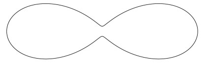
Figure 1. Non-isometric symmetrization of isometry

Figure 1 also demonstrates that convexity may be lost in the process of winding symmetrization, and thus clarifies the difference between winding symmetrization and central symmetrization [11, p. 101] which transforms closed convex curves into centrally symmetric closed convex curves.

The issue with Example 8.2 is that the curve $f(\mathbb{T})$ is too close to $0$. This distance can be controlled with the following lemma, which is well-known but is proved here for completeness.

Lemma 8.3.

Let $f\colon\mathbb{T}\to\mathbb{C}$ be an $(L,\ell)$-bi-Lipschitz embedding. Denote by $R_{I}$ the inradius of the domain $\Omega$ bounded by $f(\mathbb{T})$, that is the largest radius of a disk contained in $\Omega$. Then

(8.3) $$\ell\leq R_{I}\leq L.$$

Proof.

By the Kirszbraun theorem [7, Theorem 1.34], $f$ extends to an $L$-Lipschitz map $F\colon\mathbb{C}\to\mathbb{C}$. This extension need not be a homeomorphism, but we still have $\Omega\subset F(\mathbb{D})$ because $F_{\mathbb{T}}=f$ has nonzero degree with respect to each point of $\Omega$. It follows that every point of $\Omega$ is within distance $L$ of $F(\mathbb{T})=\partial\Omega$, which means $R_{I}\leq L$.

Similarly, extending $f^{-1}$ to an $\ell^{-1}$-Lipschitz map $G\colon\mathbb{C}\to\mathbb{C}$ we find that the inradius of $G(\Omega)$ is at most $\ell^{-1}R_{I}$. Since $G(\Omega)\supset\mathbb{D}$, the lower bound $R_{I}\geq\ell$ follows. ∎

Proposition 8.4.

Let $f\colon\mathbb{T}\to\mathbb{C}\setminus\{0\}$ be an $(L,\ell)$-bi-Lipschitz embedding. Define $r=\min_{\mathbb{T}}|f|>0$. Then the symmetrized embedding $g$, defined by (8.1), is $(\pi L,r\ell/(2\pi L))$-bi-Lipschitz.

Proof.

Outside of $0$, the map $W$ is differentiable and its derivative matrix has singular values $2$ and $1$. Hence $W$ is $2$-Lipschitz and locally invertible, with the inverse being $1$-Lipschitz. If the homeomorphism $f$ is $L$-Lipschitz, then its symmetrization $g$, which can be locally defined by $W^{-1}\circ f\circ W$, is locally $2L$-Lipschitz on $\mathbb{T}$. It follows that $g$ is $2L$-Lipschitz with respect to the path metric on $\mathbb{T}$:

(8.4) $$\lvert g(z)-g(\zeta)\rvert\leq 2L\,\rho_{\mathbb{T}}(z,\zeta)$$

where $\rho_{\mathbb{T}}(z,\zeta)$ is the infimum of lengths of curves joining $z$ to $\zeta$ and contained in $\mathbb{T}$. Since any two points $z,\zeta\in\mathbb{T}$ are joined by an arc of length at most $(\pi/2)\lvert z-\zeta\rvert$, we have $\rho_{\mathbb{T}}(z,\zeta)\leq(\pi/2)\lvert z-\zeta\rvert$, hence

$$\lvert g(z)-g(\zeta)\rvert\leq\pi L\lvert z-\zeta\rvert.$$

To prove the lower Lipschitz bound, fix $\zeta\in\mathbb{T}$. Note that $\lvert g(\zeta)\rvert\geq r$ since $W$ preserves the absolute value. Consider two cases:

Case 1. $\rho_{\mathbb{T}}(z,\zeta)\geq\pi-r/(2L)$. Then $\rho_{\mathbb{T}}(-z,\zeta)\leq r/(2L)$, which by inequality (8.4) implies $\lvert g(-z)-g(\zeta)\rvert\leq r$. Using the relation $g(-z)=-g(z)$ we obtain

$$\lvert g(z)-g(\zeta)\rvert=\lvert 2g(\zeta)+g(-z)-g(\zeta)\rvert\geq\lvert 2g(\zeta)\rvert-\lvert g(-z)-g(\zeta)\rvert\geq r\geq\frac{r}{2}\lvert z-\zeta\rvert.$$

Case 2. $\rho_{\mathbb{T}}(z,\zeta)<\pi-r/(2L)$. An elementary geometric argument shows that the restriction of $W$ to an arc of $\mathbb{T}$ of size $\beta<\pi$ has lower Lipschitz constant $2\cos(\beta/2)$ with respect to the Euclidean metric. Therefore,

$$\lvert f(W(z))-f(W(\zeta))\rvert\geq 2\ell\cos\left(\frac{\pi}{2}-\frac{r}{4L}\right)\lvert z-\zeta\rvert=2\ell\sin\left(\frac{r}{4L}\right)\lvert z-\zeta\rvert.$$

Since $f\circ W=W\circ g$ and $W$ is $2$-Lipschitz, it follows that

$$\lvert g(z)-g(\zeta)\rvert\geq\frac{1}{2}\lvert f(W(z))-f(W(\zeta))\rvert\geq\ell\sin\left(\frac{r}{4L}\right)\lvert z-\zeta\rvert.$$

The estimate $\sin x\geq 2x/\pi$, $0<x<\pi/2$, completes the proof. ∎

Remark 8.5.

The first part of the proof of Proposition 8.4 can also be applied to $g^{-1}$, showing that $g^{-1}=W^{-1}\circ f^{-1}\circ W$ is $2L$-Lipschitz with respect to the path metric on $g(\mathbb{T})$. However, this does not yield a bound on the Lipschitz constant of $g^{-1}$ in the Euclidean metric, since the shape of $g(\mathbb{T})$ is unknown.

Combining Proposition 8.4 with Lemma 8.3 we arrive at the following result.

Corollary 8.6.

For every $(L,\ell)$-bi-Lipschitz embedding $f\colon\mathbb{T}\to\mathbb{C}$ there exists a point $w_{0}\in\mathbb{C}$ such that the winding symmetrization of $f-w_{0}$ is a $(\pi L,\ell^{2}/(2\pi L))$ bi-Lipschitz map.

The point $w_{0}$ can be taken to be an incenter of the domain bounded by $f(\mathbb{T})$.

9. Conclusion

Proof of Theorem 1.1.

Given an $(L,\ell)$-bi-Lipschitz embedding $f\colon\mathbb{T}\to\mathbb{C}$, let $g$ be the winding symmetrization of $f-w_{0}$ as in Corollary 8.6. Theorem 1.1 provides its bi-Lipschitz extension $G\colon\mathbb{C}\to\mathbb{C}$ which is also centrally symmetric. Therefore there exists $F\colon\mathbb{C}\to\mathbb{C}$ such that $F\circ W=W\circ G$. Since the singular values of the derivative matrix $DW$ are $1$ and $2$, it follows that $\sup\lVert DF\rVert\leq 2\sup\lVert DG\rVert$ and $\sup\lVert DF^{-1}\rVert\leq 2\sup\lVert DG^{-1}\rVert$. Recalling the Lipschitz bounds of Corollary 8.6 and Theorem 1.2, we arrive at

$$\lVert DF\rVert\leq 2\pi\cdot 10^{27}L\leq 10^{28}L$$

and

$$\lVert DF^{-1}\rVert^{-1}\geq\frac{1}{2}\cdot 10^{-23}\frac{\ell^{2}}{2\pi L}\geq 10^{-25}\frac{\ell^{2}}{L}.$$

One of the maps $F$ and $-F$ provides the desired extension of $f$. ∎

The source of nonlinearity in Theorem 1.1 is the symmetrization process of section 8. It is thus natural to seek an form of Corollary 8.6 with a linear bound for the lower Lipschitz constant. The following example shows that such an improvement will require a better way of choosing the center point $w_{0}$ for symmetrization.

Example 9.1.

Let $f\colon\mathbb{T}\to\mathbb{C}$ be the map described by Figure 2, where $f(a)=A$, $f(b)=B$ and both boundary curves $AB$ and $BA$ are traced counterclockwise with constant speed. The Euclidean distances $\lvert a-b\rvert$ and $\lvert A-B\rvert$ are equal to a small parameter $\epsilon$. The speed at which $AB$ is traced is about $1/\epsilon$, while the speed of $BA$ is about $1$. One can see that $f$ is bi-Lipschitz with respect to the Euclidean metric with constants approximately $(1/\epsilon,1)$.

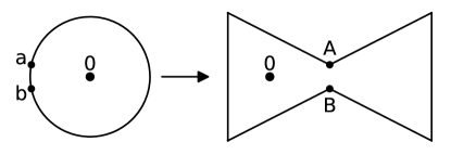
Figure 2. Bi-Lipschitz constants about $(1/\epsilon,1)$

The map obtained after winding symmetrization is shown on Figure 3. Both distances $\lvert A_{1}-B_{1}\rvert$ and $\lvert A_{2}-B_{2}\rvert$ are of order $\epsilon$. However, $\lvert a_{1}-b_{1}\rvert$ and $\lvert a_{2}-b_{2}\rvert$ are approximately $2$. Thus, the lower Lipschitz constant of the symmetrized map decays with $\epsilon$. The ratio of upper and lower Lipschitz constants gets squared in the process of winding symmetrization, as is does in Corollary 8.6.

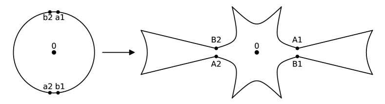
Figure 3. Bi-Lipschitz constants about $(1/\epsilon,\epsilon)$

However, if the map on Figure 2 was translated so that $0$ is in the center of the right half of the bowtie, the winding symmetrization would not incur a nonlinear growth of distortion. This motivates the following question.

Question 9.2.

Is there a universal constant $C$ such that for every $(L,\ell)$-bi-Lipschitz embedding $f\colon\mathbb{T}\to\mathbb{C}$ there exists a point $w_{0}\in\mathbb{C}$ such that the winding symmetrization of $f-w_{0}$ is a $(CL,\ell/C)$ bi-Lipschitz map?

A positive answer to Question 9.2 would provide linear distortion bounds in Theorem 1.1, thus answering the question of Daneri and Pratelli [8].

References

- [1] L. V. Ahlfors, Lectures on quasiconformal mappings, 2nd ed. Amer. Math. Soc., Providence, RI, 2006.
- [2] P. Alestalo, D. A. Trotsenko, and J. Väisälä, The linear extension property of bi-Lipschitz mappings, Sibirsk. Mat. Zh. 44 (2003), no. 6, 1226–1238; translation in Siberian Math. J. 44 (2003), no. 6, 959–968.
- [3] P. Alestalo, D. A. Trotsenko, and J. Väisälä, Plane sets allowing bilipschitz extensions, Math. Scand. 105 (2009), no. 1, 134–146.
- [4] P. Alestalo and J. Väisälä, Uniform domains of higher order. III, Ann. Acad. Sci. Fenn. Math. 22 (1997), no. 2, 445–464.
- [5] J. Azzam and R. Schul, Hard Sard: quantitative implicit function and extension theorems for Lipschitz maps. Geom. Funct. Anal. 22 (2012), no. 5, 1062–1123.
- [6] A. Beurling and L. Ahlfors, The boundary correspondence under quasiconformal mappings, Acta Math. 96 (1956), 125–142.
- [7] A. Brudnyi and Yu. Brudnyi, Methods of geometric analysis in extension and trace problems, vol. 1, Birkhäuser, 2011.
- [8] S. Daneri and A. Pratelli, A planar bi-Lipschitz extension theorem, Adv. Calc. Var. 8 (2015), no. 3, 221–266.
- [9] A. Douady and C. J. Earle, Conformally natural extension of homeomorphisms of the circle, Acta Math. 157 (1986), no. 1–2, 23–48.
- [10] P. Duren, Univalent functions, Springer-Verlag, New York, 1983.
- [11] H. G. Eggleston, Convexity, Cambridge Univ. Press, Cambridge, 1958.
- [12] J. B. Garnett and D. E. Marshall, Harmonic measure, Cambridge Univ. Press, Cambridge, 2005.
- [13] G. M. Goluzin, Geometric theory of functions of a complex variable, Translations of Mathematical Monographs, Vol. 26, American Mathematical Society, Providence, R.I.
- [14] D. S. Jerison and C. E. Kenig, Hardy spaces, , and singular integrals on chord-arc domains, Math. Scand. 50 (1982), no. 2, 221–247.
- [15] D. Kalaj, Radial extension of a bi-Lipschitz parametrization of a starlike Jordan curve, Complex Var. Elliptic Equ. 59 (2014), no. 6, 809–825.
- [16] L. V. Kovalev, Sharp distortion growth for bilipschitz extension of planar maps. Conform. Geom. Dyn. 16 (2012), 124–131.
- [17] T. G. Latfullin, Continuation of quasi-isometric mappings, Sibirsk. Mat. Zh. 24 (1983), no. 4, 212–216.
- [18] P. MacManus, Bi-Lipschitz extensions in the plane, J. Anal. Math. 66 (1995), 85–115.
- [19] Ch. Pommerenke, Univalent functions, Vandenhoeck & Ruprecht, Göttingen, 1975.
- [20] Ch. Pommerenke, Boundary behaviour of conformal maps, Springer-Verlag, Berlin, 1992.
- [21] T. Ransford, Potential theory in the complex plane, Cambridge Univ. Press, Cambridge, 1995.
- [22] D. A. Trotsenko, Extendability of classes of maps and new properties of upper sets, Complex Anal. Oper. Theory 5 (2011), no. 3, 967–984.
- [23] P. Tukia, The planar Schönflies theorem for Lipschitz maps, Ann. Acad. Sci. Fenn. Ser. A I Math. 5 (1980), no. 1, 49–72.
- [24] P. Tukia, Extension of quasisymmetric and Lipschitz embeddings of the real line into the plane, Ann. Acad. Sci. Fenn. Ser. A I Math. 86 (1981), 89–94.