Inelastic cross-section and survival probabilities at LHC in mini-jet models

Abstract

Recent results for the total and inelastic hadronic cross-sections from LHC experiments are compared with predictions from a single channel PDF driven eikonal mini-jet model and from an empirical model. The role of soft gluon resummation in the infrared region in taming the rise of mini-jets and their contribution to the increase of the total cross-sections at high energies are discussed. Survival probabilities at LHC, whose theoretical estimates range from circa 10% to a few per mille, will be estimated in this model and compared with results from QCD inspired models and from multichannel eikonal models. We revisit a previous calculation and examine the origin of these discrepancies.

I Introduction

In this paper we present an estimate of survival probabilties in hadronic collisions, obtained with the eikonal mini-jet model first proposed in Durand and Pi (1989), and later implemented with soft gluon resummation in Corsetti et al. (1996); Grau et al. (1999); Godbole et al. (2005). We shall make use of latest measurements by the TOTEM Collaboration Antchev et al. (2013a), at 7 TeV for all 3 cross-sections, and at 8 TeV in the Coulomb region and with luminosity independent measurements Antchev et al. (2016, 2013b), by CMS Chatrchyan et al. (2013a) and LHCb Aaij et al. (2015) for the inelastic cross-section at 7 TeV, by the ALICE Collaboration for the inelastic cross section at 2.76 and 7 TeV Abelev et al. (2013), by the ATLAS Collaboration for the total, inelastic and elastic $pp$ cross-sections at 7 Aad et al. (2014) and 8 TeV Aaboud et al. (2016a), and by measurements of the inelastic part at $13$ TeV by CMS Van Haevermaet (2016) and ATLAS Aaboud et al. (2016b).

Survival probabilities were originally discussed in Dokshitzer et al. (1992); Bjorken (1993) to estimate the probability associated with a hard process when no low transverse momentum particle production is present in the central region. In Bjorken (1993), such a probability was estimated to be around $5\%$ at the Superconducting Super Collider SSC ($\sqrt{s}=40$ TeV), but with an overall possible uncertainty of a factor three in either direction. Presently, for LHC data up to $\sqrt{s}=13$ TeV, estimates vary between those of a QCD inspired model Block et al. (2015) where the survival probability is calculated to be 13 %, to calculations within the Regge-Pomeron approach which range between $(0.7\div 2)\%$ in Khoze et al. (2013) and between $(0.25\div 3)\%$ in Gotsman et al. (2016). Such large discrepancies arise due to (i) the choice of the impact parameter distribution of partons involved in the scattering and, to a lesser extent, to (ii) the estimate of the inelastic total cross-section. As for data on rapidity gaps, LHC measurements at 7 TeV by ATLAS Aad et al. (2016) and CMS Chatrchyan et al. (2013b) Collaborations are affected by rather large errors and cannot yet discriminate between models.

In the following, in the quest for a clearer definition of survival probabilities (SPs), we shall employ eikonal mini-jet models to clarify and sharpen the physical meaning of the survival probability concept. Comparison with other models will also be made.

Mini-jets were first introduced in estimates of hadronic physics in Horgan and Jacob (1980); Pancheri and Rubbia (1984); Sjostrand and van Zijl (1987); Durand and Pi (1989) but were not yet recognized as dominant in proton-proton collisions when the earlier estimates of SPs appeared Bjorken (1993). Since then a better understanding of the role played by mini-jets in high energy collisions has been achieved, including proposal for beyond the leading power calculations Kotko et al. (2017).

In the following, after a brief summary of the main features of the PDF (Parton Density Function) driven mini-jet model that we employ, we examine the most recent data for the total cross-sections, and address the question of the inelastic cross-section in single channel eikonal models. We then apply our model to discuss SPs for hard and soft distributions of partons in the protons and clarify the difference arising from using different impact parameter distributions.

Revisiting a previous calculation in Achilli et al. (2008), we put forward a new proposal, which reduces the estimate of $\simeq 10\%$ at LHC energies by almost an order of magnitude. This proposal is based on the physical meaning of the survival probability concept in mini-jet models and on explicit inclusion in the calculation of the soft gluon effects accompanying mini-jet processes. Our resummation procedure is based on Poisson distributed soft gluon emissions and on an hypothesis of maximal singularity of the soft gluon spectrum.

II Accelerator data and the total $pp$ cross-section in a PDF driven eikonal model

We consider an eikonal model, such as

$$\sigma_{total}=2\int d^{2}{\bf b}[1-e^{-\chi_{I}(b,s)}]$$ (1)

where the eikonal function is taken to be purely imaginary at high energies, and contains contributions from both soft and semi-hard collisions.

For the imaginary part of the eikonal, $\chi_{I}(b,s)$, we write

$$2\chi_{I}(b,s)={\bar{n}}_{soft}(b,s)+{\bar{n}}_{hard}(b,s)=A_{FF}(b)\sigma_{soft}(s)+A_{BN}(b,s)\sigma_{mini-jet}(s,p_{tmin})$$ (2)

where $2\chi_{I}(b,s)$ can be seen to correspond to the average number of Poisson distributed parton-parton collisions Durand and Pi (1989); Achilli et al. (2011); Fagundes et al. (2015).The distinction between the two terms at the right hand side of Eq. (2) is done on the basis of using a perturbative QCD (pQCD) calculation for the mini-jet cross-section, i.e. for all interacting partons with $p_{t}\geq p_{tmin}$ Grau et al. (1999). Namely, $p_{tmin}$ is the scale of O(1-2 GeV) which phenomenologically separates collisions between partons exiting the scattering with final momenta $p_{t}>p_{tmin}$, aka mini-jets.

Hadronic activity not associated to mini-jet production can be included in ${\bar{n}}_{soft}(b,s)$, such as collisions leading to final partons with $p_{t}<p_{tmin}$. However, notice that the hadronic activity with partons with $p_{t}<p_{tmin}$ can come both through ${\bar{n}}_{hard}(b,s)$ and ${\bar{n}}_{soft}(b,s)$, because of the soft gluon emission accompanying the hard (mini-jet) processes, as we shall describe below. We should also point out that the two-component separation of Eq. (2) misses to include Single Diffraction, which has an energy dependence different from the mini-jet cross-section. We shall return to this point later in the paper.

The term, ${\bar{n}}_{hard}(b,s)$, is obtained from QCD, with the distribution $A_{BN}(b,s)$ to describe the contribution of soft gluon emission accompanying collisions between partons with final momenta $p_{t}>p_{tmin}$. The subscript $BN$ refers to our choice of exploiting the full range of soft gluon momenta, down to $k_{t}=0$, in the spirit of the Bloch and Nordsieck description of soft quanta emission in QED Bloch and Nordsieck (1937). Our application to QCD has been described in a number of previous publications, starting from Nakamura et al. (1984a) until recently in Fagundes et al. (2015), where we provide details about our calculation of ${\bar{n}}_{hard}(b,s)$. In Eq. (2) both $A_{FF}(b)$ and $A_{BN}(b,s)$ are normalized to 1.

Together with soft gluon resummation, to which we shall turn shortly, the distinctive element of our model is that the mini-jet cross-section is not parametrized but calculated (at Leading Order (LO)) from the QCD standard expression, and with standard PDFs, DGLAP evoluted, $f_{i|A}(x_{1},p_{t}^{2})$, i.e.

$$\sigma^{AB}_{\rm jet}(s;p_{t_{min}})=\int_{p_{tmin}}^{\sqrt{s}/2}dp_{t}\int_{4p_{t}^{2}/s}^{1}dx_{1}\int_{4p_{t}^{2}/(x_{1}s)}^{1}dx_{2}\sum_{i,j,k,l}f_{i|A}(x_{1},p_{t}^{2})f_{j|B}(x_{2},p_{t}^{2})~{}~{}\frac{d\hat{\sigma}_{ij}^{kl}(\hat{s})}{dp_{t}}.$$ (3)

with $i,\ j,\ k,\ l$ to denote the partons and $x_{1},\ x_{2}$ the fractions of the parent particle momentum carried by the parton. $\sqrt{\hat{s}}=\sqrt{x_{1}x_{2}s}$, $\hat{\sigma}$ are the center of mass energy of the two parton system and the hard parton scattering cross–section respectively. Following the argument given above, this expression sums only collisions with outgoing partons of momentum with $p_{t}>p_{tmin}$, where $p_{tmin}$ is defined as the region of validity of perturbative QCD, i.e. the coupling is given by the asymptotic freedom expression for running $\alpha_{s}(p^{2}_{t})$. When the cut-off $p_{tmin}\gtrsim 1-2$ GeV, it is usual to refer to these type of processes as mini-jets Horgan and Jacob (1980).

The result of our calculation is shown in Fig.  1 for three different LO PDF sets, together with presently available data for the total cross-section Antchev et al. (2016); Aaboud et al. (2016a); Aad et al. (2014); Abreu et al. (2012); Abbasi et al. (2015).

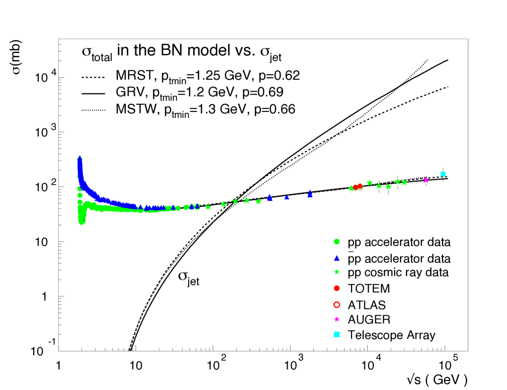
Figure 1: The figure shows how the mini-jet cross-section compares with presently available data for $\sigma_{total}$. The continuous, dashed and dotted curves correspond to three different parton density functions, such as Glück, Reya and Vogt (GRV) Glück et al. (1998, 1992), Martin, Roberts, Stirling and Thorne (MRST) Martin et al. (1998) and Martin, Stirling, Thorne and Watt (MSTW) Martin et al. (2009). The corresponding curves over the total cross-section data are obtained with the BN model referred to in the text.

The comparison between the energy rise of $\sigma_{jet}(s;p_{tmin})$, [from here on, the terms jet and mini-jet are used interchangeably], and the actual total cross-section highlights the well known fact that, around ISR energies, hard QCD collsions, as calculated to LO, start becoming important, but then rising too much. This difficulty is solved in the BN model by dressing the mini-jet cross-section with the phenomenon of soft gluon emission which dampens the rise of the parton-parton cross-sections, and embedding them in the formalism of eikonalization, which ensures unitarity. Soft gluon emission in impact parameter space then provides the large distance cut-off which allows satisfaction of the Froissart bound Grau et al. (2009). For partial completeness, we shall outline here the main points of our approach to resummation of soft gluon emission in hadronic process.

II.1 Soft gluon resummation in the infrared region

Together with the PDF driven mini-jet contribution, the core feature of our working model lies in the impact parameter distribution of the pQCD term, $A_{BN}(b,s)$, which was obtained as the Fourier transform of the resummed probability for soft gluon emissions accompanying any QCD scattering process. As we discuss next, the subscript $BN$ refers to our choice of exploiting the full range of soft gluon momenta, down to $k_{t}=0$, in the spirit of the Bloch and Nordsieck description of soft quanta emission.

For the resummed soft gluon distribution, we had proposed Corsetti et al. (1996) to start from the semi-classical expression Etim et al. (1967)

$$\Pi(K_{t},s)=\int\frac{d^{2}{\bf b}}{(2\pi)^{2}}e^{-i{\bf K}_{t}\cdot{\bf b}-h(b,s)}$$ (4)

$$h(b,s)=\int d^{3}{\bar{n}}({\bf k},s)[1-e^{i{\bf k}_{\perp}\cdot{\bf b}}]$$ (5)

with $d^{3}{\bar{n}}({\bf k})$ being the single soft quantum spectrum, which is exponentiated and regularized through resummation. Eqs. (4) and (5) exhibit a crucial result of the resummation technique developed in Etim et al. (1967), i.e. the cancellation at semi-classical level of the QED singularities arising from infrared emission and virtual exchanges. Such cancellation follows from imposing energy-momentum conservation to resummation of soft quanta emitted through Poisson distributions, as we outline in Appendix A.

Unlike $\Pi(K_{t},s)$, which can be obtained through a semiclassical calculation, the application of the above technique to elementary particle processes requires the spectrum $d^{3}{\bar{n}}({\bf k})$ to be determined from quantum field theory, in particular from QCD, in the case of soft gluon emission.

Within the context of the Bloch-Nordsieck approach, one can find an early discussion of the probability distribution $\Pi(K_{t},s)$ for particle production in strong interactions with a constant large coupling in Pancheri-Srivastava and Srivastava (1977). Applied to Drell-Yan production processes, the QCD case of running $\alpha_{s}$ was examined in Dokshitzer et al. (1978) and Soper and Collins (1981) in the Leading Logarithmic Approximation, and by Parisi and Petronzio (PP) Parisi and Petronzio (1979) within the context of the Bloch-Nordsieck approach. In particular, the expression proposed in Parisi and Petronzio (1979) for the function $h(b,s)$ reads:

$$h^{(PP)}(b,s)=\frac{4}{3\pi^{2}}\int_{M^{2}}^{Q^{2}}d^{2}{\bf k}_{\perp}[1-e^{i{\bf k}_{\perp}\cdot{\bf b}}]\alpha_{s}(k_{\perp}^{2})\frac{\ln(Q^{2}/k_{\perp}^{2})}{k_{\perp}^{2}}$$ (6)

with a lower limit of integration $M^{2}\neq 0$ and using the asymptotic freedom expression for $\alpha_{s}$. The contribution of the infrared region, $k_{\perp}^{2}\leq M^{2}$ was incorporated in an intrinsic transverse momentum factor, with the assumption that the neglected terms coming from this region would not have a singular behavior which could affect the result.

On the other hand, our long held proposal Nakamura et al. (1984b); Corsetti et al. (1996) is to calculate the probability resummation function $\Pi(K_{t},s)$ down into the infrared region, as relevant to the large $b$-behaviour of the total cross-section, since this is a region where a singular behavior might manifest itself, through a confining potential. Thus, in our approach the single gluon spectrum depends on the coupling $\alpha_{IR}(k_{t})$ in the infrared region. Our modeling of such behavior has been discussed in many papers, in particular we have a thorough discussion in Grau et al. (1999) and Pancheri and Srivastava (2017).

Let $\Lambda$ be an infrared scale separating the asymptotic freedom QCD regime from the non perturbative one, then our phenomenological ansatz for the coupling as $k_{t}\rightarrow 0$ Nakamura et al. (1984b); Corsetti et al. (1996), leads to

$$\alpha_{IR}(k_{t})\propto[\frac{\Lambda}{k_{t}}]^{2p}\ \ \ \ \ \ \ \ k_{t}<<\Lambda$$ (7)

The above limit can be justified by a semi-classical argument about confining potentials Nakamura et al. (1984b); Grau et al. (1999), and the parameter $p$ could be considered as parametrizing such complex processes as resummation of multi soft gluon couplings. For integrability of the rhs in Eq. (5) on the one hand, and for a correspondence to a rising potential on the other, the parameter $p$ is limited to the range $1/2<p<1$ Grau et al. (2009).

With such ansatz for $\alpha_{s}(k_{t}\rightarrow 0)$, one can calculate the function $h(b,s)$ down into the infrared region. The final calculation of the normalized function $A_{BN}(b,s)$, with the subscript BN to indicate the resummation approach we follow, is done by choosing an appropriate value for the singularity parameter $p$ and specifying the upper limit of integration in Eq. (5), appropriate to the perturbative QCD processes of mini-jets. Calling it ${q_{max}}$, it represents the maximum momentum allowed to single gluon emission; it depends on the energy distribution of the emitting partons (hence on the PDFs), and the perturbative parton-parton cross-section (it was Drell-Yan in Parisi and Petronzio (1979)), and ultimately from $p_{tmin}$. In our simplified realization of this model, $q_{max}$ is obtained from the expression proposed in Chiappetta and Greco (1981) as discussed in Grau et al. (1999).

One can then proceed to calculate the average number of hard collisions for the BN model as

$${\bar{n}}_{hard}(b,s)=A_{BN}(b,s)\sigma^{pp}_{\rm jet}(s;p_{tmin})=\frac{e^{-h(b,s)}}{\int d^{2}{\bf b}e^{-h(b,s)}}\sigma^{pp}_{\rm jet}(s;p_{tmin})$$ (8)

In Fig. 2 we show the distribution $A_{BN}(b,s)$ for different c.m.energies of the $pp$ system, and compare it with an often used impact parameter distribution in total cross-section calculation, namely the convolution of proton form factors

$$A_{FF}(b)=\frac{\mu^{2}}{96\pi}(\mu b)^{3}K_{3}(\mu b)\\$$ (9)

with $\mu^{2}=0.71$ GeV. In the figure, two different parametrizations of the PDFs are used to calculate $q_{max}$ (and hence $A_{BN}(b,s)$), MSTW and GRV. The point of interest is two-fold here : for central collisions, i.e. $b\simeq 0$, the form factor type distribution (dot-dashed curve) is much lower than for the mini-jet process, whereas only a proton form factor type distribution survives at large $b$ values.

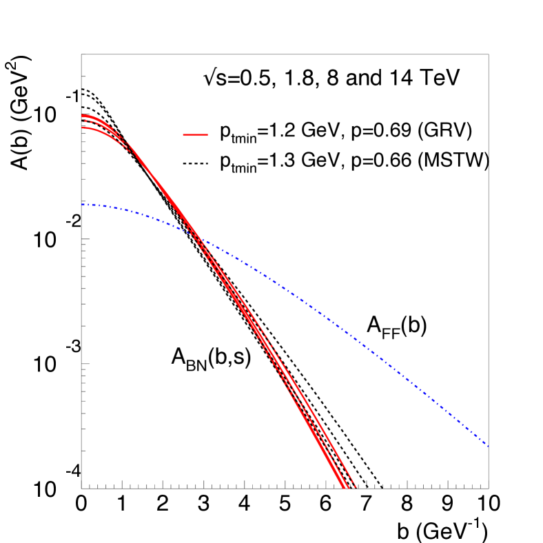
Figure 2: The dot-dashed line shows the normalized impact parameter distribution obtained from the convolution of proton form factors, compared with the BN model for two different PDFs, and parameters as indicated. As the energy increases, the distributions in the MSTW case (black dashes) shift more and more towards $b=0$, whereas GRV curves (full red) flatten out, with 8 and 14 TeV curves practically indistinguishable.

II.2 The total cross-section in the BN model

As well known, and as apparent from Fig. 1, the mini-jet contributions, with their energy dependence, are not sufficient to describe the normalization of the total cross-section. Total cross-section data at low energy, i.e. $\sqrt{s}\leq 5\div 10$ GeV, suggest to include an additional contribution which can be given, in this model, by the term ${\bar{n}}_{soft}$ as in Eq.  (2), with $\sigma_{soft}(s)$ parametrized through a best fit to the total cross-section, as

$$\sigma_{soft}(s)=48.2+\frac{101.66}{E_{lab}^{0.99}}-\frac{27.89}{E_{lab}^{0.59}}\ \ \ \ (mb)$$ (10)

The reader would note that in Godbole et al. (2005) a different parametrization of ${\bar{n}}_{soft}$ had been proposed. We leave to a forthcoming paper a discussion of these two different approaches.

We now see that the calculation of the total cross-section in the BN model, depends on two different sets of parameters: those extracted from the low-energy regime, with $\sigma_{soft}$ described by a constant and one or more decreasing powers in energy, and those for the high energy region, the latter being: (i) the choice of the PDFs, (ii) the separation scale between hard and soft processes, $p_{tmin}$, and (iii) the infrared parameter $p$. The high energy set characterizes the energy behavior of the total cross-section as it increases with energy, a behavior driven by QCD mini-jets but regulated by soft gluon emission, modeled by the parameter $p$, as $k_{t}^{single-gluon}\rightarrow 0$.

We also notice, in Fig.  1, that the different trend of the mini-jet cross-sections in the high energy region, due to the small-x behavior of the parton-parton cross-section from different PDFs, is much smoothed down in the total cross-section. This is due to the interplay between mini-jet rise and the accompanying soft gluon emission which dampens it. Such interplay enters through the maximum single gluon momentum $q_{max}$ which is proportional to $p_{tmin}$, the fixed mini-jet scale. The dependence on densities and $p_{tmin}$ however is not eliminated completely. This appears clearly in Fig.  3, where the actual calculation of the total cross-section from Eq. (1) is presented in a linear-log scale (rather than log-log as in Fig. 1).

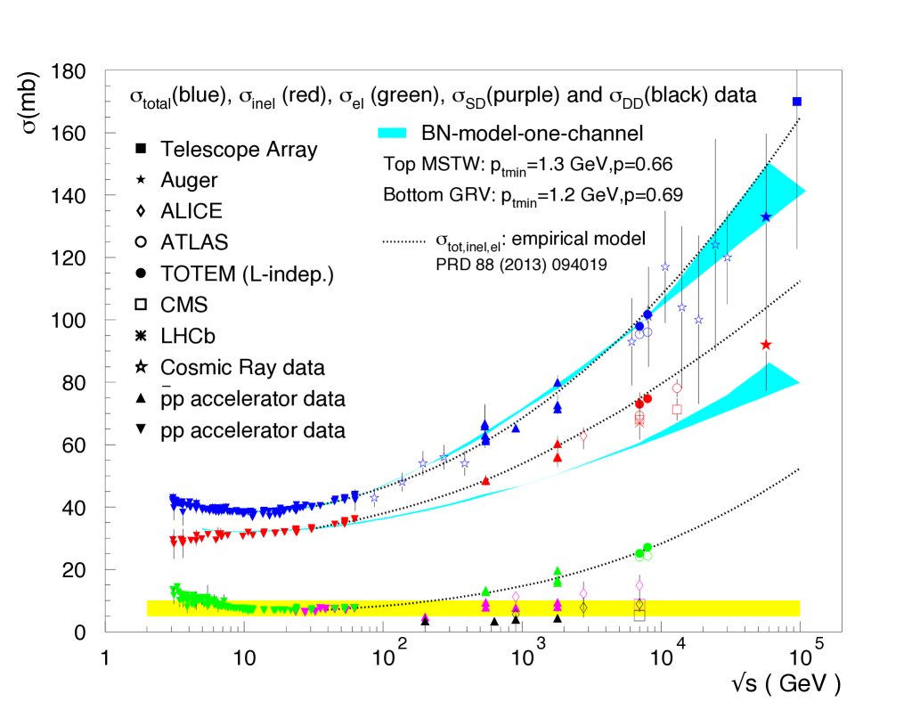
Figure 3: The figure shows the band of expected results for the total and inelastic cross-section for the BN model for two sets of PDFs, and predictions from the empirical model of Fagundes et al. (2013) for total, elastic and inelastic cross-sections. For the inelastic cross-section, only data with extrapolation to the full phase space are shown. Other data and references for the inelastic cross-section measurements at LHC are summarized in Table 1. For a comparison, diffractive data are also shown, with a constant yellow band to guide the eye.

As discussed and seen in Fagundes et al. (2015), tuning of the parameters leads to an optimal description of the total cross-section data up to $\sqrt{s}=7$ and $8$ TeV, both using “old” densities, such as GRV, as well as using more recent parametrizations such as MSTW. However, the small-x behavior of the parton-parton cross-section still leads to $(10\div 20)\%$ uncertainties when extrapolation is done to higher energies such as those reachable through cosmic ray experiments.

In the next subsection, we shall discuss the other data and curves appearing in this figure.

II.3 The inelastic cross-sections

For estimates of the survival probabilities Bjorken (1993), the quantity of interest is the inelastic cross-section in impact parameter space. In single channel models this can be obtained through the elastic amplitude

$${\cal F}(s,t)=i\ \int bdbJ_{o}(qb)[1-e^{-\chi_{I}(b,s)}]\\$$ (11)

with $q^{2}=-t$,namely from the equation

$$\sigma_{inelastic}=\int d^{2}{\bf b}[1-e^{-2\chi_{I}(b,s)}]\equiv\int d^{2}{\bf b}[1-P_{no-inel}(b,s)]$$ (12)

with

$$P_{no-inel}(b,s)=e^{-{\bar{n}}(b,s)}\equiv e^{-{\bar{n}}_{soft}(b,s)-{\bar{n}}_{hard}(b,s)}$$ (13)

in a two-component eikonal as described before. However one problem arises: as discussed in Fagundes et al. (2015) and clearly seen in Fig. 3 the inelastic cross-section obtained from Eqs. (12) and (13), and estimated with the parameters leading to the good description of $\sigma_{total}$, reproduces LHC inelastic data only in a limited range, $\xi=M^{2}_{X}/s\gtrsim 5\times 10^{-6}$ falling short of the full phase space extrapolated data.

A model independent estimate of the inelastic cross-section is shown by the dotted lines in Fig. 3. This estimate is obtained as $\sigma_{inel}=\sigma_{tot}^{emp}-\sigma_{el}^{emp}$ by mean of an empirical parametrization of all the differential $pp$ cross-section data from ISR to LHC, based on the elastic amplitude

$${\cal A}(s,t)=i[F^{2}_{P}(t/t_{0})\sqrt{A(s)}e^{B(s)t/2}+e^{i\phi(s)}\sqrt{C(s)}e^{D(s)t/2}]$$ (14)

where $F^{2}_{P}(t)$ is the square of the proton form factor, i.e. $F_{P}(t/t_{0})=1/[(1+|t|/t_{0})]^{2}$. Details of this model, which is a modified version of the 1974 Phillips and Barger proposal Phillips and Barger (1973), can be found in Fagundes et al. (2013) and are reproduced here in the Appendix B. For a new version of the model, now augmented to describe the $\rho$ parameter, see Ruiz Arriola and Broniowski (2017).

Thus, the empirical model applied to the inelastic cross-section confirms the extrapolations to the full phase space as obtained through MC simulations or other models. At the same time, the single channel two-component BN model, we just described, has so far not included energy dependent diffraction processes. Data for these type of events are displayed in Fig. 3, respectively from ISR Armitage et al. (1982), UA5 Ansorge et al. (1986), UA4 Bernard et al. (1987), CDFAbe et al. (1994), Abelev et al. (2013) and CMSKhachatryan et al. (2015).

One obvious missing element in the single channel model we have proposed is Single Diffraction. As seen from Fig. 3, this process, unlike Double Diffraction, shows an energy dependence characteristic of QCD processes, namely its contribution increases with energy. Indeed, while the BNmodel so far includes QCD processes such as gluon-gluon collisions and the accompanying resummed soft gluon emission, it misses one more process which can give energy dependence to the cross-section through perturbative QCD, namely hard gluon bremsstrahlung from the proton and its accompanying soft gluon emission, as well. This process, at the origin of Single Diffraction contributions, is correlated to the emitting proton and its inclusion in a single-channel model has so far been difficult.

However, lacking a clear understanding of diffraction in mini-jet type models, we propose that the quantity $P_{no-inel}$ thus calculated can be used to estimate survival probabilities when Single Diffractive events are not excluded, and proceed to do so in the next section.

We conclude this section with a comparison of our single channel BN model with recent experimental results for the inelastic cross-section, in the measured phase regions, as shown in Table 1.

Table 1: The inelastic cross-section at LHC obtained from the single channel two-component BN model, and its comparison with existing data at LHC and cosmic ray energies. The last column shows the estimate obtained (by subtraction) from the empirical model of Fagundes et al. (2013).

$\sqrt{s}$	$\sigma_{inel}$	Kinematic range	Experiment	$\sigma_{inel}^{BN}$	Emp.
TeV	mb	$\xi_{X}=M^{2}_{X}/s$		mb	mb
		and $\xi_{Y}=M^{2}_{Y}/s$		GRV-MSTW	Fagundes et al. (2013)
2.76	$62.8^{+2.7}_{-4.2}$	full- sim.	ALICE Abelev et al. (2013)
7		no SD		59.8-60.5
	$60.3\pm 0.5(syst)\pm 2.1(lum)$	$\xi_{X}>5\times 10^{-6}$	ATLAS Aad et al. (2011)
	$60.2\pm 0.2(stat)\pm 1.1(sys)\pm 2.4(lum)$	$\xi_{X}>5\times 10^{-6}$	CMS Chatrchyan et al. (2013a)
	$62.1^{+1.0}_{-0.9}(sys)\pm 2.2(lum)$	$\xi_{X}>5\times 10^{-6}$	ALICE Abelev et al. (2013)
	$55.0\pm 2.4$	$p_{T}>0.2GeV/c,2.0<\eta<4.5$	LHCb Aaij et al. (2015)
	$71.34\pm 0.36(stat)\pm 0.83(syst)$	full-by subtraction	ATLAS Aad et al. (2014)		74.8
	$72.9\pm 1.5$	lum-independent -full	TOTEM Antchev et al. (2013a)
	$68.0\pm 4.0(model)\pm 2.0(sys)\pm 2.4(lum)$	full-MC simu;	CMS Zsigmond (2012)
	$66.9\pm 2.9(exp)\pm 4.4(extr)$	full-Pythia 6	LHCb Aaij et al. (2015)
	$73.2^{+2.0}_{-4.6}(model)\pm 2.6(lum)$	full -diff model	ALICE Abelev et al. (2013)
8		no SD		60.7-62.1
	$74.7\pm 1.7$	full-MC simul.	TOTEM Antchev et al. (2013b)
	$71.73\pm 0.15(stat)\pm 0.69(sys)$	full-by subtraction	ATLAS Aaboud et al. (2016a)		76.6
13		no SD		64.3- 66.6
	$65.77\pm 0.03(stat)\pm 0.76(sys)\pm 1.78(lum)$	HF $\xi>10^{-6}$	CMS Van Haevermaet (2016)
	$68.1\pm 0.6(exp)\pm 1.3(lum)$	$\xi>10^{-6}$	ATLAS Aaboud et al. (2016b)
	$66.85\pm 0.06(stat)\pm 0.44(sys)\pm 1.96(lum)$	HF+CASTOR $\xi_{X}>10^{-7},\xi_{Y}>10^{-6}$	CMS Van Haevermaet (2016)
	$71.26\pm 0.06(stat)\pm 0.47(sys)\pm 2.09(lum)\pm 2.72(ext)$	extr. all models	CMS Van Haevermaet (2016)
	$78.1\pm 0.6(exp)\pm 1.3(lum)\pm 2.6(ext)$	extr. - full	ATLAS Aaboud et al. (2016b)		82.9
14		No SD		64.8- 67.4
14					83.9
57		No SD		75.6-85.4
$57$	$92\pm^{13.4}_{14.8}$	full-from Glauber and other effects	AUGER Abreu et al. (2012)		103.8

III Survival Probabilities

Let us recall early discussions of survival probability Dokshitzer et al. (1992); Bjorken (1993) that arose in considerations of a hadronic collision at an impact parameter $b$ producing a final state characterized by energy scales much larger than those of the soft and semi-hard background of hadronic collision. Such a final state can be high $p_{t}$ jet pair production, or Higgs production, for instance, and, we look for events with no hadronic activity in the central region.

Let $S^{2}(b,s)$ be the distribution for observing one such high $p_{t}$ process with cross-section $\sigma_{hard-scale}(s)$ and no additional inelastic collisions Bjorken (1993). A simplified factorized model for such distribution can be written as

$$S^{2}(b,s)=\sigma_{hard-scale}^{AB}(s){\cal H}(b,s)P_{no-collisions}(b,s)$$ (15)

where ${\cal H}(b,s)$ is the distribution in impact parameter space of those partons participating to the collision leading to the production of H (the hard-scale process). Then the distribution $S^{2}(b,s)$ can be integrated and normalized and the average survival probability distribution is obtained from the simplified expression

$${\cal S}^{2}(s)\equiv<|S(b,s)|^{2}>=\int d^{2}{\bf b}A(b,s)e^{-{\bar{n}}(b,s)}$$ (16)

having used Eq. (13) and with

$$A(b,s)=\frac{{\cal H}(b,s)}{\int d^{2}{\bf b}{\cal H}(b,s)}$$ (17)

Leaving aside for the time being the question of the missing piece of the inelastic cross-section in single channel eikonal minjet models such as the one described earlier, we can write

$$P_{no-collisions}(b,s)=P_{no-soft-collisions}(b,s)P_{no-mini-jets}(b,s)$$ (18)

where the first factor on the r.h.s. excludes the presence of soft partons from events for which the cross-section is either constant or decreasing. This term alone does not exclude production of mini-jets. Instead, these processes, which can be described by perturbative QCD, as we have seen, and constitute the hadronic background for which partons exit the collision with $p_{t}>p_{tmin}\simeq 1\ GeV$ accompanied by the infrared initial state emission, are suppressed through the factor $P_{no-mini-jets}(b,s)=exp[-{\bar{n}}_{mini-jets}(b,s)]$.

In cases where one puts a $p_{t}$-cut (say, 1 GeV) to eliminate the mini-jet emission (as when the hard process to select is production of a color singlet, for instance), one would have to consider

$$S^{2}(b,s)=\sigma_{hard-scale}^{AB}(s){\cal H}^{mini-jets}(b,s)P_{no-mini-jets}(b,s)$$ (19)

but notice that not all low $p_{t}$ activity is excluded, since some hadronic activity from ${\bar{n}}_{soft}(b,s)$ has not been excluded.

If absence of both soft collisions and mini-jets is required, then one should use the full probability $P_{no-collisions}(b,s)$ as in Eq. (15). We shall now address the question as to which impact parameter distribution is appropriate to a given measurement. In what follows, we shall see what is involved in such calculations and compare with existing model predictions.

III.1 SP results from BN-2008 and Block et al.-2015 estimate from QCD inspired models

Let us start with SP estimates from the BN model, as done originally in 2008 Achilli et al. (2008) and revisit it in order to compare with (2015) results from Block and collaborators Block et al. (2015). For quark initiated processes, the total survival probability of the gap in this QCD inspired model is obtained from the expression

$$<|S(b)|^{2}>=\int d^{2}{\bf b}A(b,\mu_{qq})e^{-2\chi_{I}(b,s)}$$ (20)

with $A(b,\mu_{qq})$ the distribution of quarks in the proton, for which the relative parton-parton cross-section is decreasing. In this single channel eikonal model Block et al. (1992, 1999), $\chi_{I}(b,s)$ is obtained as the contribution from three terms: gluon-gluon, quark-gluon and quark-quark collisions, i.e.

$$\chi_{I}(b,s)=W(\mu_{gg})\sigma_{gg}(s)+W(\mu_{qg})\sigma_{qg}(s)+W(\mu_{qq})\sigma_{qq}(s)$$ (21)

with $W(\mu)$ obtained from a convolution of dipoles, and different scales $\mu_{ij}$ in correspondence with three basic cross-sections $\sigma_{ij}$, with different energy behaviors. These parameters were tuned to the large set of elastic and total cross-section data available before the LHC operation. As we shall see in more detail later, this model predicts rather large survival probabilities at LHC when compared with recent estimates from the Durham-St. Petersburg group, Khoze, Martin and Ryskin (KMR) in Khoze et al. (2013) and those from the Telaviv group of Gotsman, Levin and Maor (GLM) in Gotsman et al. (2016). In the following, we shall attempt to understand this difference.

Our earlier estimate of survival probabilities Achilli et al. (2008) was similar to a previous one by Block and Halzen Block and Halzen (2001), but we now believe that such estimates should be reconsidered. To understand why (and how), we notice that in Achilli et al. (2008) our estimate was done using

$$<|S(b)|^{2}>=\int d^{2}{\bf b}A_{soft}(b,s)e^{-2\chi_{I}(b,s)}$$ (22)

with $A_{soft}(b,s)$ obtained as the distribution of partons with final $p_{t}<p_{tmin}$ in correspondance with non mini-jet collisions. Following our present parametrization of ${\bar{n}}_{soft}(b,s)$, we now evaluate Eq. (22) using the convolution of proton form factors as discussed in the previous section, and the updated parametrization for $\chi_{I}(b,s)$ which led to the curves for the total cross-section in Fig. 3. With this procedure, which we can call the BN-2008 model for the survival probability, we show in Fig. 4 the agreement between the recent Block and collaborators results and the estimate from Eq. (22).

The reason for the approximate agreement between our calculation and the recent Block et al. result, lies in the very similar role played by the two distributions $A(b,\mu_{qq})$ and $A_{soft}(b)$ entering Eqs. (20) and (22): they both correspond to parton processes whose cross-section is not rising with energy. At the same time, in both models, $P_{no-inel}$ is constructed with contributions from both rising and constant parton cross sections, with an eikonal such as to reproduce the total cross-section. In the BN model, the decomposition of collisions corresponds to two types of soft hadronic activity, one coming from processes in which the production of soft partons is energy independent or decreasing, and one with mini-jet production [dressed with infra-red gluons whose number is increasing with energy] that drives the rise of the total cross-section. In a similar way, the Aspen model, used for the estimate in Block et al. (2015), includes three types of contributions, with $gg$ and $gq$ rising with energy, and $qq$ constant or decreasing.

However, this way to estimate the survival probability certainly needs revision for the following reason. To exclude all hadronic background processes which at high energy show an increase with energy, one needs to take into account the rising contribution from mini-jets or semi-hard collisions from partons whose $b$-distribution is very different, as shown in Fig. 2 for the BN model.

These estimates are also compared in Fig. 4 with the result by Bjorken at $\sqrt{s}=40$ TeV Bjorken (1993), where the lowest value was obtained with a multiplicative model (red line), as we summarize below.

Considering only independent collisions, and an expression as in Eq. (20), Bjorken estimated the survival probability to be about 10%, with numerical estimates from Block et al. (1992), and under the assumption of uncorrelated parton distributions.

However, when Bjorken included the possibility of hadronic activity clustered around the valence quarks, he suggested instead the following:

$$<|S|^{2}>_{Bj}\simeq\frac{\int d^{2}{\vec{B}}F(B)|S_{pp}(B)|^{2}\int d^{2}{\vec{b}}\ \sigma_{qq}^{Hard}|S_{qq}(b)|^{2}}{\int\ d^{2}{\vec{B}}F(B)\int d^{2}{\vec{b}\ \sigma_{qq}^{Hard}(b)}}=<|S|^{2}>_{pp}<|S|^{2}>_{qq}$$ (23)

where $<|S|^{2}>_{pp}$ is the survival probability estimated before, whereas $<|S|^{2}>_{qq}$ is an extra factor. The additional term could exclude collisions rising with energy and hadronic activity correlated with the valence quarks alone. In any case, an additional diminution of the survival probability was expected and a value of 5% was considered more likely (red dot in the figure), with a factor 3 uncertainty in either direction. This is what we have shown in the figure.

A comparison is also shown with the LO result by the CMS collaboration Chatrchyan et al. (2013b) for the survival probability in the measurement of the diffractive contribution to dijet production at $\sqrt{s}=7\ TeV$. CMS gives an estimate of $S^{2}=0.12\pm 0.05$ at LO, and a lower value of $S^{2}=0.08\pm 0.04$ at NLO. A similar more recent (2015) measurement by the ATLAS collaboration Aad et al. (2016), not shown in the plot, uses an estimate of $S^{2}=0.16\pm 0.04(stat)\pm 0.08(exp.syst)$ for dijet production in $\sqrt{s}=$ 7 TeV $pp$ collisions with large rapidity gaps, this estimate being considered to be also consistent with a central value of $0.15$.

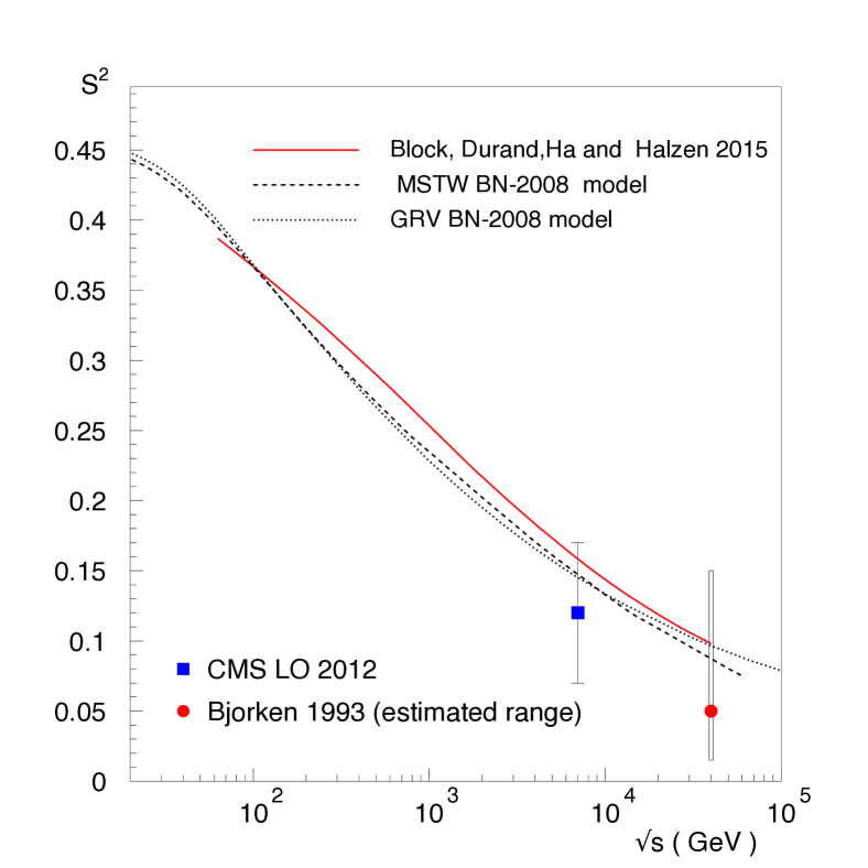
Figure 4: We show the survival probabilities obtained with the soft process impact parameter distributions from Block et al. (2015) (full line) and the BN model in Achilli et al. (2008), compared with the Bjorken’s estimate at 40 TeV Bjorken (1993), based on an impact parameter using a soft distribution first and then a multiplicative model for hard processes. We also show the LO estimate by CMS Chatrchyan et al. (2013b).

In the next subsection, we shall present a different proposal, in which first a split is made between soft and hard contributions and then, the fractioned (lack of) hadronic activity from each is summed to construct the SP. We shall compare -with plots and tables- our calculation with the Telaviv and Durham-St Petersburg models, labelled here, for short, as GLM and KMR.

III.2 Our proposal with all order resummation of soft gluons

Let us approach the calculation of the survival probability in a single channel two-component eikonal model such as our BN model, in which one splits the eikonal into a component rising with energy, and another component either constant or decreasing.

To exclude all hadronic uncorrelated activity, one can distinguish between $soft$ and $hard$ collisions as participating with different weights to the survival probability,

$$w_{soft/hard}(s)\equiv\frac{\sigma_{soft/jet}(s)}{\sigma_{soft}(s)+\sigma_{jet}(s)}\equiv\frac{\sigma_{soft/jet}(s)}{\sigma_{B}(s)}$$ (24)

with $\sigma_{B}$ to represent the “Born term” of the total cross-section, $\sigma_{jet}$ being obtained from Eq. (3) and $\sigma_{soft}$ from Eq. (10). As one can see from Fig. 1 , at low energy, $w_{soft}>>w_{hard}$, while their roles are exchanged at high energy. Then the contribution to the survival probability will depend on the relative weights as follows:

• in the case of emission coming from processes with a cross-section not rising with energy and final hadrons with $p_{t}<p_{tmin}$, in our phenomenological approach

  • (i) the $b-$distribution is given by $A_{FF}(b)$, namely follows the form factor distribution, with no extra energy dependence,

  • (ii) the probability of no such emission is given by $e^{-{\bar{n}}_{soft}}$,

  • (iii) the survival probability is obtained as

    $$<|S(b)|^{2}>_{soft}=\int d^{2}{\bf b}A_{FF}(b,s)e^{-{\bar{n}}_{soft}(b,s)}$$

• in the case of QCD mini-jet processes, for which final hadrons have $p_{t}>p_{tmin}$ and an increasing rising cross-section, the b-distribution is obtained through soft gluon emission accompanying the mini-jet collision, and

  $$<|S(b)|^{2}>_{hard}=\int d^{2}{\bf b}A_{BN}(b,s)e^{-{\bar{n}}_{hard}(b,s)}$$

Our proposal is that the survival probability -to exclude hadronic activity in the central region- is given by

$$\bar{\mathcal{S}}^{2}_{total}(s)=\bar{\mathcal{S}}^{2}_{soft}(s)+\bar{\mathcal{S}}^{2}_{hard}(s)\equiv w_{soft}(s)<|S(b)|^{2}>_{soft}+w_{hard}(s)<|S(b)|^{2}>_{hard}$$ (25)

With the caveat that diffractive events are either poorly or not at all described by the single channel model and hence are not excluded by $P_{no-inel}$, we now proceed to calculate the survival probabilities and compare it with other models.

We present the results of our proposal in Table 2 for the two types of densities used to describe the inelastic (and hence the total) cross-section,

Table 2: Survival probabilities, soft, hard and total, in the TeV region, in the additive model we propose, using MSTW densities ($p_{tmin}=1.3$ GeV and $p=0.66$), and GRV ($p_{tmin}=1.2$ GeV and $p=0.69$). All values are given in percentages, with the values taken by $\bar{\mathcal{S}}^{2}_{total}$ plotted Fig. 5.

$\sqrt{s}$	$\bar{\mathcal{S}}^{2}_{soft}$		$\bar{\mathcal{S}}^{2}_{hard}$		$\bar{\mathcal{S}}^{2}_{total}$
TeV	GRV	MSTW	GRV	MSTW	GRV	MSTW
1.8	3.17	4.77	1.53	2.70	4.70	7.47
2.76	2.15	3.38	1.06	1.95	3.21	5.33
7.0	0.942	1.32	0.490	0.810	1.43	2.13
8.0	0.839	1.17	0.440	0.722	1.28	1.89
13	0.554	0.681	0.297	0.433	0.851	1.11
14	0.526	0.669	0.282	0.425	0.808	1.03
40	0.222	0.182	0.124	0.121	0.346	0.303

and show in Fig. 5 the values taken by $\bar{\mathcal{S}}^{2}_{total}$ for GRV and MSTW densities, in comparison with GLM and KMR estimated ranges. We also show comparison with the NLO CMS estimate Chatrchyan et al. (2013b). Since our present proposal is obtained by resummation of soft gluons to all orders, the comparison with NLO result is the appropriate one. Please notice the change in scales.

Figure 5: The (black and red) curves indicate the estimated Survival Probabily Rapidity Gaps (in percentage) in the LHC region, in the additive model we propose in Eq. (25), using impact parameter distributions obtained from the BN model for the mini-jet component, with MSTW (dashes) or GRV (full) LO PDFs, with all order Soft Gluon (SG) resummation. Comparison with ranges estimated in the models by GLM (cyan band) and KMR (yellow band), and with LHC measurements at 7 TeV by CMS at NLO Chatrchyan et al. (2013b) is also shown.

These results are now summarized in Table 3, and Fig. 6, where we compare our proposal with the experimental estimates by ATLAS and CMS collaborations, with those by Block, Durand, Ha and Halzen, the two Reggon-Pomeron models we have mentioned, and the 40 TeV range of values estimated by Bjorken Bjorken (1993). For the BN model, we also show the separate estimates for $\bar{\mathcal{S}}^{2}_{soft}$ and $\bar{\mathcal{S}}^{2}_{hard}$.

Table 3: Survival probability predictions of the models by Block-Durand-Ha-Halzen (BDHH) Block et al. (2015), Khoze-Martin-Ryskin (KMR) Khoze et al. (2013) and Gotsman-Levin-Maor (GLM) Gotsman et al. (2016), and the range of prediction by Bjorken (BJ) Bjorken (1993). All values are given in percentages.The BN model range includes calculation with two different PDFs.

$\sqrt{s}$	$\bar{\mathcal{S}}^{2}_{BDHH}$	$\bar{\mathcal{S}}^{2}_{KMR}$	$\bar{\mathcal{S}}^{2}_{GLM}$	$\bar{\mathcal{S}}^{2}_{BN}(I)$	$\bar{\mathcal{S}}^{2}_{BJ}$
TeV				GRV-MSTW
0.063	38.7 $\pm$ 0.6	$8.7-20.8\ (10)$	$-$
0.546	28.6 $\pm$ 0.5	$4.1-10.3\ (4.7)$	$-$
0.630	27.8 $\pm$ 0.5	$-$	$-$
1.8	22.2 $\pm$ 0.5	$2.3-6.3\ (2.8)$	$0.86-7.6\ (3.34)$	4.70 - 7.47
7.0	$-$	$1.1-3.2\ (1.5)$	$0.3-3.63\ (3.1)$	1.43-2.13
13				0.851-1.11
14	13.1 $\pm$ 0.3	$0.7-2.2\ (1.0)$	$0.25-2.3\ (3.05)$	0.808-1.03
40	9.8 $\pm$ 0.2	$-$	$-$	0.346 - 0.303	1.5-15 (5)

Figure 6: Comparison of the predictions for the survival probability gaps estimates (in percentage) in the context of the BN model, with other models described in the text and with CMS Chatrchyan et al. (2013b) and ATLAS Aad et al. (2016) measurements at LHC7.

As already discussed our estimate is close to Block’s only when the soft distribution, which we take to be the folding of two proton form factors, is used. On the other hand, we find our results to be consistent with the range of values coming from different models by the Durham Khoze et al. (2013) and Telaviv group Gotsman et al. (2016).

In the table, the Durham model results are obtained using the GW formalism in a two channel eikonal model, which includes low mass diffractive dissociation, and is able to predict both elastic and diffractive cross-sections. Four different models are discussed, all of which give similar good fit to the various cross-sections, but have different values for $|S|^{2}$. The difference is ascribed to depend on the details of the Good and Walker splitting and hence to the impact parameter density of the GW states. The authors’ favored model is indicated between parentheses and corresponds to energy dependent coupling of the triple Pomeron.

The table also displays a band of prediction for GLM, such as given by the values in Table 3 of Ref. Gotsman et al. (2016). In this case the values in parenthesis represent the model for which new parameters of their model were provided (Model IIn) - the ones describing the total, elastic and diffractive cross sections (low and high mass) at LHC. As emphasized by them that model gives higher values for the survival probability. The spread in values given by the Telaviv group depends on the impact parameter distribution of the hard amplitude, with a Gaussian $e^{-b^{2}/4B}$ behaviour , which leads to the correct Froissart limit, and on different sets of parameters (called “new” and “old”), and also on the inclusion of kinematics corrections. This work develops in the context of a CGC/saturation approach for soft interactions at high energy and is detailed in Ref.Gotsman et al. (2016).

On the other hand, it is rather clear what our present single-channel model can predict. The integrand in Eq. (16) depends on two quantities:

1. $P_{no-inelastic}$ which is fixed by the fit to the total cross-section, i.e. in single channel by the function $\chi_{I}(b,s)$ which describes $\sigma_{total}(s)$; in our interpretation, missing part or all of diffraction, $P_{no-inelastic}\equiv P_{only-diffractive-events}$

2. the impact parameter distribution of partons which can come from either soft collisions, with $A_{FF}(b)$, or hard, mini-jet collisions, with $A_{BN}(b,s)$. In our single channel eikonal, we have seen in Grau et al. (2009) that $A_{BN}(b,s)\sim e^{-(b\bar{\lambda})^{2p}}$. With the singularity parameter $1/2<p<1$ [our phenomenology indicates $p\simeq(0.6\div 0.7)$], one can see that the cut off in b-space is midway between a gaussian and an exponential, leading to an asymptotic behavior of the total cross-section $\sigma_{total}\lesssim[\ln s]^{1/p}$, satisfying the Froissart bound. Please notice that an improvement of the Froissart limit in the context of the AdS/CFT correspondence has recently been proposed in Errasti Diez et al. (2015).

From this discussion, it is not completely clear which model gives the best representation for the survival probabilities. While we are convinced that previous estimates of survival probabilities through mini-jet or QCD inspired models should be calculated using our proposal Eq. (25) rather than Eq. (20) or (22), at the same time we are aware of the limitations of the single-channel model. We expect that full exclusion of the hadronic background may further reduce the survival probability.

IV Final comments and conclusions

The survival probability concept implies the need to be able to select processes which are unaccompanied by the usual hadronic activity. This may be useful for a selected process such as Higgs production, high $p_{t}$ jets, or any hard process which one wants to isolate from the background. The quantity to look for is therefore a no-collision probability which is characterized by the presence of rapidity gaps, around the central region. Such quantity is easily calculated in the eikonal formulation. However, the single channel formulation of the inelastic cross-section given in Eq. (12) fails to reproduce the totality of the inelastic cross-section, as the energy increases towards LHC regime. At energies lower than those attained at LHC, data for the full inelastic cross-section are obtained by subtraction from two well measured quantities, the total and the elastic, i.e. $\sigma_{inel}=\sigma_{total}-\sigma_{el}$. This quantity includes events with different topologies, distinguished in various groups, such as soft, hard diffraction, and central diffraction. The contribution from processes in the very forward direction is not uniquely measurable by the different experiments, and data are provided in terms of the covered phase space or through model extrapolations.

Here we propose that the least ambiguous way to use the concept of survival probability is through selecting events which do not have hadronic activity outside the diffractive region. In early release of elastic cross-section data at LHC, a common phase space limitation $\xi=M_{X}^{2}/s\geq 5\times 10^{-6}$ was shown to be well described by a single channel model such as ours. Therefore one can now turn this fact around and define this region as the one for which the present single channel BN model can provide an estimate for the survival rapidity gaps in the central region. Namely, if ${\bar{n}}(b,s)\equiv 2\chi_{I}(b,s)$ is chosen so as to describe the total cross-section, then

$$P_{no-inel}(b,s)=e^{-{\bar{n}}(b,s)}$$ (26)

gives the probability distribution for no independently distributed collisions at impact parameter value $b$, and given c.m. energy. The survival probability at any given impact value $b$ is then dependent on the density of partons in the overlapping area in b-space. For central collisions, the hadronic matter is denser (confinement dilutes gluonic matter in the peripheral regions) and vice versa for the peripheral collisions. By integrating the probability of no collisions with the hadronic matter distribution in the hadron, we have calculated the survival probability [for the case in which Single Diffraction is not excluded] and found an estimate of $\sim 1\%$ at LHC8 and LHC13.

The result we have presented obtains through an all order resummation procedure applied to soft gluon emission in mini-jet collisions.

Finally, we notice that results similar to the ones we are proposing for the BN model, can be expected in the model of Block et al. Block and Halzen (2001) when this model is applied using our prescription.

Appendix A Derivation of semi-classical resummation formula

In this Appendix, we present a derivation of Eq. (4) following Etim et al. (1967). In the scattering of high energy charged particles, a considerable portion of the energy is radiated away in the form of of either hard or soft radiation, photons in QED, gluons in QCD. In this appendix, we shall outline the method of soft quanta resummation we use in QCD.

When a charged particle is bent in its path by the electromagnetic field, the cloud of soft photons accompanying the motion of the charged particle is not affected by the external field and continues its path, tangent to the trajectory at the point when the charged particle entered the bending field. This is true in QED where the external field has no effect on the soft photons surrounding the traveling electron, but it is more difficult to see it in QCD. However, this is true also in this case, because of the infrared catastrophe, as can be seen through a reading of the Block and Nordsieck theorem Bloch and Nordsieck (1937) which demonstrates that only the emission of an infinite number of soft photons has a finite probability. This argument can be applied as well to soft gluon emission, being based on ignoring the recoil of the emitting particles and summing of all the Poisson distributed number of soft quanta. Thus in the emission, when the gluon energy goes to zero, the number of emitted gluons is infinite and the emitted energy accompanying this infinite number of gluons is color neutral and the soft gluon cohort does not interact with the external field.

In the language of quantum field theory, we can describe the process of soft gluon emission as a process in which straightforward perturbation theory does not apply in the sense that only the emitted energy-momentum is a finite quantity, not the single soft gluons. In order to resum this infinite number of soft gluons (or soft quanta emitted by a charged source) we can start from the theory of emission from a classical source as given by Bloch and Nordsieck, in which the distribution of soft photons is shown to be given by a Poisson distribution, i.e.

$$P(\{n_{\bf k}\})=\Pi_{\bf k}\frac{[{\bar{n}}_{\bf k}]^{n_{\bf k}}}{n_{\bf k}!}e^{-{\bar{n}}_{\bf k}}$$ (27)

where $P(\{n_{\bf k}\})$ can now be taken to corresponds to the probability that the emitted massless quanta are emitted with $n_{{\bf k}_{1}}$ gluons with momentum ${\bf k}_{1}$, $n_{{\bf k}_{2}}$ gluons with momentum ${\bf k}_{2}$, etc. The next step is to consider the overall energy-momentum loss $K$ accompanying the scattering and impose energy-momentum conservation to the sum of all the possible Poisson distributions, i.e.

$$d^{4}P(K)=\sum_{n_{\bf k^{\prime}}}P(\{n_{\bf k^{\prime}}\})\delta^{4}(\sum_{k^{\prime}}k^{\prime}{n_{\bf k^{\prime}}}-K)d^{4}K$$ (28)

The sum over all the distributions runs again along the lines of a classical derivation, using the four-dimension integral representation of the $\delta$ function, which allows to exchange the order of product of distributions and their summation. One thus reaches the expression

$$d^{4}P(K)=\frac{d^{4}K}{(2\pi)^{4}}\int d^{4}x\ e^{-h(x)+iK\cdot x}$$ (29)

with

$$h(x)=\sum_{k}(1-e^{-ik\cdot x}){\bar{n}}_{\bf k}$$ (30)

Going from the discrete to the continuum limit and integrating Eqs. (29) and(30) on the unobserved variables of energy $K_{0}$ and longitudinal momentum $K_{3}$, one obtains Eq. (4). The derivation can be applied to gluons or photons, provided the resulting integrand in Eq. (6) be an integrable function. In QED this quantity is not just integrable but is also finite. The QCD limit is discussed in the text, with the proposal, put forward in Nakamura et al. (1984b), that the integrand in Eq. (6) be singular but integrable. This leads to the condition that the infrared limit of the soft gluon coupling to the emitting source be no more singular than $(k_{\perp}^{2})^{-p}$ with $p<1$ and to the adoption of this limit in the phenomenological approach, which we have called the BN model.

Appendix B The full inelastic cross-section from the empirical model

For the case when background emission in a wider phase space has to be excluded, a simple way to estimate the full inelastic cross-section can be obtained from the empirical model of Fagundes et al. (2013). We present here the results of this model, although we shall not use it to estimate the survival probabilities, in absence of a clear indication of how to calculate the impact parameter distribution of partons to associate to this model. We consider an empirical model based on the improved parametrization of the elastic amplitude following the Phillips and Barger Phillips and Barger (1973) proposal. As TOTEM data Antchev et al. (2011) for the differential elastic cross-section appeared, we discussed the validity of this model in Grau et al. (2012) and, in Fagundes et al. (2013), we revised it, proposing two different modifications, labelled $mBP1$ and $mBP2$, aimed to ameliorate the description of the amplitude at $t=0$, and obtain a better fit of the total cross-section.

Our improved expression is based on a best fit to all $pp$ differential cross-section data from ISR energies up to $\sqrt{s}=7$ TeV, using a parametrization of the elastic amplitude, which, in the $mBP2$ version of the empirical model, was proposed to be

$${\cal A}(s,t)=i[F^{2}_{P}(t/t_{0})\sqrt{A(s)}e^{B(s)t/2}+e^{i\phi(s)}\sqrt{C(s)}e^{D(s)t/2}]$$ (31)

where $F^{2}_{P}(t)$ is the square of the proton form factor, i.e. $F_{P}(t/t_{0})=1/[(1+|t|/t_{0})]^{2}$ with $t_{0}$ a parameter with weak energy dependence, approaching $0.7\ GeV^{2}$ at high energies. The introduction of this factor in the first term at the right hand side of Eq.  (31) modifies the Phillips and Barger proposal to give a better agreement with total cross-section data.

This model has 6 real parameters: two amplitudes, $A(s)$ and $C(s)$, two slopes, $B(s)$ and $D(s)$, one phase $\phi$ and one scale $t_{0}$. The model was able to give an excellent description of available data up to $\sqrt{s}=7$ TeV, and can be used to extrapolate to higher energies. Using the full range of ISR and LHC7 data, we can make predictions for the two amplitudes and the two slopes at higher energies by means of asymptotic theorems. As for the phase and the scale, while the phase was kept constant, for the energy dependence of $t_{0}(s)$ we use the interpolation/extrapolation fit result: $t_{0}=0.66+15.4/\log^{2}(s/1\ \text{GeV}^{2})$, which gives a good description of the $t_{0}$ parameter in Fagundes et al. (2013). The values we propose to be used for the parameters in the LHC energy range are given in Table 4.

Using the amplitude of Eq. (31) and the asymptotic projections for the two amplitudes $A(s),\ C(s)$ and the two slopes $B(s)$ and $D(s)$, we calculate the total cross-section at much higher than present energies, and compare it with data. And then, always from the above amplitude, one can also calculate and predict values for the elastic total cross-section, and, by default, for the inelastic, $\sigma_{inel}^{emp}=\sigma_{tot}^{emp}-\sigma_{el}^{emp}$. These expectations are shown as dotted lines in Fig. 3.

We see that both the elastic and the total cross-section are well described by the empirical model parametrization at all energies - in fact the 8 TeV TOTEM values for the total cross-section is correctly predicted to be 103 mb vs. the TOTEM value at 102.9 mb - while the inelastic cross-section appears slightly higher than the TOTEM data and clearly higher than CMS.

Table 4: Energy evolution of the mBP2 empirical model parameters used in Fig. 3. We have assumed a nearly constant phase, $\phi\simeq 2.9$ rad, throughout in our calculations.

$\sqrt{s}$ (TeV)	A (mbGeV2)	B (GeV-2)	C (mbGeV2)	D (GeV-2)	$t_{0}$ (GeV2)
0.5	197	4.83	0.217	3.19	0.760
2.0	344	6.50	0.693	4.00	0.727
8.0	597	8.78	1.30	4.80	0.708
13	719	9.71	1.51	5.08	0.703
20	846	10.6	1.69	5.33	0.699
50	1180	12.6	2.06	5.87	0.693

References

- Durand and Pi (1989) L. Durand and H. Pi, Phys. Rev. D40, 1436 (1989).
- Corsetti et al. (1996) A. Corsetti, A. Grau, G. Pancheri, and Y. N. Srivastava, Phys. Lett. B382, 282 (1996), arXiv:hep-ph/9605314 .
- Grau et al. (1999) A. Grau, G. Pancheri, and Y. Srivastava, Phys.Rev. D60, 114020 (1999), arXiv:hep-ph/9905228 [hep-ph] .
- Godbole et al. (2005) R. M. Godbole, A. Grau, G. Pancheri, and Y. N. Srivastava, Phys. Rev. D72, 076001 (2005), arXiv:hep-ph/0408355 [hep-ph] .
- Antchev et al. (2013a) G. Antchev et al. (TOTEM), Europhys. Lett. 101, 21004 (2013a).
- Antchev et al. (2016) G. Antchev et al. (TOTEM), Eur. Phys. J. C76, 661 (2016), arXiv:1610.00603 [nucl-ex] .
- Antchev et al. (2013b) G. Antchev et al. (TOTEM), Phys. Rev. Lett. 111, 012001 (2013b).
- Chatrchyan et al. (2013a) S. Chatrchyan et al. (CMS), Phys. Lett. B722, 5 (2013a), arXiv:1210.6718 [hep-ex] .
- Aaij et al. (2015) R. Aaij et al. (LHCb), JHEP 02, 129 (2015), arXiv:1412.2500 [hep-ex] .
- Abelev et al. (2013) B. Abelev et al. (ALICE), Eur. Phys. J. C73, 2456 (2013), arXiv:1208.4968 [hep-ex] .
- Aad et al. (2014) G. Aad et al. (ATLAS), Nucl. Phys. B889, 486 (2014), arXiv:1408.5778 [hep-ex] .
- Aaboud et al. (2016a) M. Aaboud et al. (ATLAS), Phys. Lett. B761, 158 (2016a), arXiv:1607.06605 [hep-ex] .
- Van Haevermaet (2016) H. Van Haevermaet (CMS), Proceedings, 24th International Workshop on Deep-Inelastic Scattering and Related Subjects (DIS 2016): Hamburg, Germany, April 11-15, 2016, PoS DIS2016, 198 (2016), arXiv:1607.02033 [hep-ex] .
- Aaboud et al. (2016b) M. Aaboud et al. (ATLAS), Phys. Rev. Lett. 117, 182002 (2016b), arXiv:1606.02625 [hep-ex] .
- Dokshitzer et al. (1992) Y. L. Dokshitzer, V. A. Khoze, and T. Sjostrand, Phys. Lett. B274, 116 (1992).
- Bjorken (1993) J. D. Bjorken, Phys. Rev. D47, 101 (1993).
- Block et al. (2015) M. M. Block, L. Durand, P. Ha, and F. Halzen, Phys. Rev. D92, 014030 (2015), arXiv:1505.04842 [hep-ph] .
- Khoze et al. (2013) V. A. Khoze, A. D. Martin, and M. G. Ryskin, Eur. Phys. J. C73, 2503 (2013), arXiv:1306.2149 [hep-ph] .
- Gotsman et al. (2016) E. Gotsman, E. Levin, and U. Maor, Eur. Phys. J. C76, 177 (2016), arXiv:1510.07249 [hep-ph] .
- Aad et al. (2016) G. Aad et al. (ATLAS), Phys. Lett. B754, 214 (2016), arXiv:1511.00502 [hep-ex] .
- Chatrchyan et al. (2013b) S. Chatrchyan et al. (CMS), Phys. Rev. D87, 012006 (2013b), arXiv:1209.1805 [hep-ex] .
- Horgan and Jacob (1980) R. Horgan and M. Jacob, in CERN School Phys.1980:65 (1980) p. 65.
- Pancheri and Rubbia (1984) G. Pancheri and C. Rubbia, Nucl. Phys. A418, 117c (1984).
- Sjostrand and van Zijl (1987) T. Sjostrand and M. van Zijl, Phys. Rev. D36, 2019 (1987).
- Kotko et al. (2017) P. Kotko, A. M. Stasto, and M. Strikman, Phys. Rev. D95, 054009 (2017), arXiv:1608.00523 [hep-ph] .
- Achilli et al. (2008) A. Achilli, R. Hegde, R. M. Godbole, A. Grau, G. Pancheri, and Y. Srivastava, Phys. Lett. B659, 137 (2008), arXiv:0708.3626 [hep-ph] .
- Achilli et al. (2011) A. Achilli, R. M. Godbole, A. Grau, G. Pancheri, O. Shekhovtsova, et al., Phys.Rev. D84, 094009 (2011), arXiv:1102.1949 [hep-ph] .
- Fagundes et al. (2015) D. A. Fagundes, A. Grau, G. Pancheri, Y. N. Srivastava, and O. Shekhovtsova, Phys. Rev. D91, 114011 (2015), arXiv:1504.04890 [hep-ph] .
- Bloch and Nordsieck (1937) F. Bloch and A. Nordsieck, Phys. Rev. 52, 54 (1937).
- Nakamura et al. (1984a) A. Nakamura, G. Pancheri, and Y. N. Srivastava, Phys. Rev. D29, 1936 (1984a).
- Abreu et al. (2012) P. Abreu et al. (Pierre Auger), Phys. Rev. Lett. 109, 062002 (2012), arXiv:1208.1520 [hep-ex] .
- Abbasi et al. (2015) R. U. Abbasi et al. (Telescope Array), Phys. Rev. D92, 032007 (2015), arXiv:1505.01860 [astro-ph.HE] .
- Glück et al. (1998) M. Glück, E. Reya, and A. Vogt, Eur. Phys. J. C5, 461 (1998), arXiv:hep-ph/9806404 [hep-ph] .
- Glück et al. (1992) M. Glück, E. Reya, and A. Vogt, Z. Phys. C53, 127 (1992).
- Martin et al. (1998) A. D. Martin, R. G. Roberts, W. J. Stirling, and R. S. Thorne, Eur. Phys. J. C4, 463 (1998), arXiv:hep-ph/9803445 [hep-ph] .
- Martin et al. (2009) A. D. Martin, W. J. Stirling, R. S. Thorne, and G. Watt, Eur. Phys. J. C63, 189 (2009), arXiv:0901.0002 [hep-ph] .
- Grau et al. (2009) A. Grau, R. M. Godbole, G. Pancheri, and Y. N. Srivastava, Phys. Lett. B682, 55 (2009), arXiv:0908.1426 [hep-ph] .
- Etim et al. (1967) G. Etim, G. Pancheri, and B. F. Touschek, Nuovo Cim. 51B, 276 (1967).
- Pancheri-Srivastava and Srivastava (1977) G. Pancheri-Srivastava and Y. Srivastava, Phys. Rev. D15, 2915 (1977).
- Dokshitzer et al. (1978) Y. L. Dokshitzer, D. Diakonov, and S. I. Troian, Phys. Lett. B79, 269 (1978).
- Soper and Collins (1981) D. E. Soper and J. C. Collins, Proceedings, 20th International Conference on High-Energy Physics: Madison, Wisconsin, July 17-23, 1980, AIP Conf. Proc. 68, 185 (1981).
- Parisi and Petronzio (1979) G. Parisi and R. Petronzio, Nucl. Phys. B154, 427 (1979).
- Nakamura et al. (1984b) A. Nakamura, G. Pancheri, and Y. N. Srivastava, Z. Phys. C21, 243 (1984b).
- Pancheri and Srivastava (2017) G. Pancheri and Y. N. Srivastava, Eur. Phys. J. C77, 150 (2017), arXiv:1610.10038 [hep-ph] .
- Chiappetta and Greco (1981) P. Chiappetta and M. Greco, Phys. Lett. B106, 219 (1981), [Erratum: Phys. Lett.B107,456(1981)].
- Fagundes et al. (2013) D. A. Fagundes, A. Grau, S. Pacetti, G. Pancheri, and Y. N. Srivastava, Phys. Rev. D88, 094019 (2013), arXiv:1306.0452 [hep-ph] .
- Phillips and Barger (1973) R. Phillips and V. D. Barger, Phys.Lett. B46, 412 (1973).
- Ruiz Arriola and Broniowski (2017) E. Ruiz Arriola and W. Broniowski, Phys. Rev. D95, 074030 (2017), arXiv:1609.05597 [nucl-th] .
- Armitage et al. (1982) J. C. M. Armitage et al., Nucl. Phys. B194, 365 (1982).
- Ansorge et al. (1986) R. E. Ansorge et al. (UA5), Z. Phys. C33, 175 (1986).
- Bernard et al. (1987) D. Bernard et al. (UA4), Phys. Lett. B186, 227 (1987).
- Abe et al. (1994) F. Abe et al. (CDF), Phys. Rev. D50, 5535 (1994).
- Khachatryan et al. (2015) V. Khachatryan et al. (CMS), Phys. Rev. D92, 012003 (2015), arXiv:1503.08689 [hep-ex] .
- Aad et al. (2011) G. Aad et al. (ATLAS), Nature Commun. 2, 463 (2011), arXiv:1104.0326 [hep-ex] .
- Zsigmond (2012) A. J. Zsigmond (CMS), in Proceedings, 20th International Workshop on Deep-Inelastic Scattering and Related Subjects (DIS 2012): Bonn, Germany, March 26-30, 2012 (2012) pp. 781–784, arXiv:1205.3142 [hep-ex] .
- Block et al. (1992) M. M. Block, F. Halzen, and B. Margolis, Phys. Rev. D45, 839 (1992).
- Block et al. (1999) M. M. Block, E. M. Gregores, F. Halzen, and G. Pancheri, Phys. Rev. D60, 054024 (1999), arXiv:hep-ph/9809403 [hep-ph] .
- Block and Halzen (2001) M. M. Block and F. Halzen, Phys. Rev. D63, 114004 (2001), arXiv:hep-ph/0101022 [hep-ph] .
- Errasti Diez et al. (2015) V. Errasti Diez, R. M. Godbole, and A. Sinha, Phys. Lett. B746, 285 (2015), arXiv:1504.05754 [hep-ph] .
- Antchev et al. (2011) G. Antchev et al. (TOTEM), Europhys. Lett. 95, 41001 (2011), arXiv:1110.1385 [hep-ex] .
- Grau et al. (2012) A. Grau, S. Pacetti, G. Pancheri, and Y. N. Srivastava, Phys. Lett. B714, 70 (2012), arXiv:1206.1076 [hep-ph] .