Effects of Turbulence on the Critical Conditions of Explosion

How Turbulence Enables Core-Collapse Supernova Explosions

Abstract

An important result in core-collapse supernova (CCSN) theory is that spherically-symmetric, one-dimensional simulations routinely fail to explode, yet multi-dimensional simulations often explode. Numerical investigations suggest that turbulence eases the condition for explosion, but how is not fully understood. We develop a turbulence model for neutrino-driven convection, and show that this turbulence model reduces the condition for explosions by about 30%, in concordance with multi-dimensional simulations. In addition, we identify which turbulent terms enable explosions. Contrary to prior suggestions, turbulent ram pressure is not the dominant factor in reducing the condition for explosion. Instead, there are many contributing factors, ram pressure being only one of them, but the dominant factor is turbulent dissipation (TD). Primarily, TD provides extra heating, adding significant thermal pressure, and reducing the condition for explosion. The source of this TD power is turbulent kinetic energy, which ultimately derives its energy from the higher potential of an unstable convective profile. Investigating a turbulence model in conjunction with an explosion condition enables insight that is difficult to glean from merely analyzing complex multi-dimensional simulations. An explosion condition presents a clear diagnostic to explain why stars explode, and the turbulence model allows us to explore how turbulence enables explosion. Though we find that turbulent dissipation is a significant contributor to successful supernova explosions, it is important to note that this work is to some extent qualitative. Therefore, we suggest ways to further verify and validate our predictions with multi-dimensional simulations.

1 Introduction

Understanding how massive stars end their lives still remains an important astrophysical problem. Observations indicate that most massive stars likely explode as core-collapse supernovae (Li et al., 2011; Horiuchi et al., 2011), but the theoretical details of the explosion mechanism are still uncertain. The most certain part of the theory is that the Fe core collapses, bounces at nuclear densities forming a proto-neutron star, and launches a shock wave (Janka et al., 2016). However, this shock wave quickly stalls (Hillebrandt & Mueller, 1981; Mazurek, 1982; Mazurek et al., 1982). For over three decades, the most prominent mechanism has been the delayed-neutrino mechanism in which neutrinos reheat the matter below the stalled shock and relaunch it into an explosive blast wave (Bethe & Wilson, 1985). For all but the least massive stars, the neutrino mechanism fails in one-dimensional, spherically-symmetric simulations (Liebendörfer et al., 2001b, a, 2005; Rampp & Janka, 2002; Buras et al., 2003; Thompson et al., 2003; Kitaura et al., 2006; Buras et al., 2006a; Radice et al., 2017) but multi-dimensional simulations do explode (Herant et al., 1994; Janka & Müller, 1995; Burrows et al., 1995; Janka & Müller, 1996; Burrows et al., 2007; Melson et al., 2015; Dolence et al., 2015; Müller, 2016; Roberts et al., 2016; Bruenn et al., 2016) and initial analyses suggest that multi-dimensional instabilities and turbulence aid the neutrino mechanism toward explosion (Murphy & Burrows, 2008; Marek & Janka, 2009; Murphy & Meakin, 2011a; Hanke et al., 2012; Murphy et al., 2013; Radice et al., 2016; Couch & Ott, 2015; Melson et al., 2015). Therefore, understanding the explosion mechanism requires an understanding of the conditions between failed and successful explosions and how turbulence aids the explosion. There appears to be a critical condition for explosion (Burrows & Goshy, 1993; Murphy & Burrows, 2008; Murphy & Dolence, 2017), and the critical condition for explosion is easier to obtain in multi-dimensional simulations (Herant et al., 1994; Janka & Müller, 1995, 1996; Burrows et al., 1995; Murphy & Burrows, 2008; Melson et al., 2015). In this manuscript, we propose an analytic model for turbulence and investigate how it reduces the condition for explosion.

For a thorough review on the status and problems of CCSN theory, see Müller (2017) and Janka et al. (2016). Here, we motivate our work with some of the most salient points. We know that the core collapses, but not yet how the collapse reverses into explosion. Whether a massive star explodes or not, the Fe core collapses at the end of the massive star’s life. Prior to collapse, the overlying Si-burning layer adds Fe onto the iron core. As the iron core grows in size, the electrons which supply much of the electron degeneracy pressure become more and more relativistic. As the core nears the Chandrasekhar mass limit, the relativistic electron degeneracy pressure becomes less effective at supporting the core against gravitational collapse. Meanwhile, neutrino losses reduce the lepton number, decreasing the number of electrons available to supply pressure. The iron core becomes gravitationally unstable and contracts down to a sea of nucleons, forming a proto-neutron star, and is thus supported mostly by the strong force. At these nuclear densities, the equation of state for the core stiffens, and the core abruptly bounces, slamming into the rest of the star which is collapsing supersonically onto the bouncing proto-neutron star. This creates an outward moving shock wave. As the shock wave propagates outward, it loses energy via photodissociation of Fe, electron capture, and neutrino losses. The shock stalls into an accretion shock, but if the star is to explode, this stalled accretion shock must relaunch into an explosive blast wave.

One proposed solution to relaunching the blast wave was the delayed-neutrino mechanism (Bethe & Wilson, 1985). During the stalled shock phase, the neutron star is cooling with a neutrino luminosity of a few $\times$ $10^{52}$ ergs/s, but only about 10% of this luminosity is recaptured in a net heating region, the gain region. This volume is above the proto-neutron star but below the shock. If neutrino heating were the only effect, then this would be sufficient to relaunch the explosion. However, the region below the shock is in sonic contact, and so the structure satisfies a boundary-value problem. While the neutrino heating adds heat that would drive explosion, the neutrino cooling at the base and the ram pressure of matter accreting through the shock keeps the shock stalled. The hope has been that for high enough neutrino luminosities or low accretion rates, the neutrinos may overwhelm the ram pressure and relaunch the explosion. Alas, spherically symmetric simulations show that this mechanism fails in in all but the least massive progenitors (Liebendörfer et al., 2001b, a, 2005; Rampp & Janka, 2002; Buras et al., 2003; Thompson et al., 2003; Kitaura et al., 2006; Buras et al., 2006a; Müller et al., 2017; Radice et al., 2017).

While one-dimensional simulations fail, many multi-dimensional simulations seem to succeed (sometimes weakly) (Herant et al., 1994; Janka & Müller, 1995; Burrows et al., 1995; Janka & Müller, 1996; Burrows et al., 2007; Melson et al., 2015; Dolence et al., 2015; Müller, 2016; Roberts et al., 2016; Bruenn et al., 2016; Burrows et al., 2016), and the best indications are that turbulence plays an important role in aiding the delayed-neutrino mechanism toward explosion (Bethe & Wilson, 1985; Janka & Müller, 1996; Marek & Janka, 2009; Murphy et al., 2013; Murphy & Meakin, 2011a). Therefore, to truly understand the explosion mechanism of massive stars, we need to identify the conditions for explosion and how turbulence affects these conditions.

There are many attempts to characterize these conditions, some are empirical (O’Connor & Ott, 2011; Ott et al., 2013; Ertl et al., 2016), some are heuristic (Janka & Keil, 1998; Thompson, 2000; Thompson et al., 2005; Buras et al., 2006b; Müller et al., 2016), and others attempt to derive a condition from fundamentals (Burrows & Goshy, 1993; Pejcha & Thompson, 2012; Murphy & Dolence, 2017). Of these, the most illuminating to date has been the neutrino-luminosity and accretion-rate critical curve (Burrows & Goshy, 1993). During the stalled shock phase, Burrows & Goshy (1993) noted that one may derive steady-state solutions for the stalled shock structure. The governing equations describe a boundary value problem in which the lower boundary is set by the neutron star surface (the neutrino-sphere) and the outer boundary is the shock. They parameterized the problem in terms of the accretion rate, $\dot{\mathcal{M}}$, onto the shock, and the neutrino luminosity, $L_{\nu}$, emanating from the core. In this two-dimensional parameter space they found steady-state solutions below a critical curve. Above this curve, they did not find steady-state stalled solutions, and suggested, but did not prove, that the solutions above the critical neutrino-luminosity and accretion-rate curve are dynamic and explosive.

Murphy & Dolence (2017) take a step closer to proving that the solutions above the curve are explosive by showing that the only steady solutions above this curve indeed have a positive shock velocity ($v_{s}>0$). Burrows & Goshy (1993) focused on just $\dot{\mathcal{M}}$ and $L_{\nu}$, but there are five parameters that define the steady solutions. They are neutrino luminosity ($L_{\nu}$), mass accretion rate ($\dot{\mathcal{M}}$), neutron star mass ($M_{NS}$), neutron star radius ($R_{NS}$), and the neutrino temperature ($T_{\nu}$). Murphy & Dolence (2017) point out that the critical condition is not a critical curve but a critical hypersurface; most importantly, they find that this critical hypersurface is described by one dimensionless parameter, $\Psi$. In essence, $\Psi$ is an integral condition related to the balance of pressure and gravity behind the shock. For a given set of the five parameters, $\Psi$ may be negative, zero, or positive, which correspond to $v_{s}<0$, $v_{s}=0$, and $v_{s}>0$. There is always a minimum $\Psi$, and if $\Psi_{\rm min}<0$, then there is always a stable steady-state stalled solution such that $\Psi=0$. The critical condition is where $\Psi_{\rm min}=0$. Above this critical condition, $\Psi_{\rm min}>0$, and all steady solutions have $v_{s}>0$. Assuming that these $v_{s}>0$ steady solutions correspond to explosion, they use $\Psi_{\rm min}$ to define an explodability parameter.

Using one- and two-dimensional simulations Murphy & Burrows (2008), empirically confirmed that criticality is a useful condition for explosion in core-collapse simulations. Furthermore, they found that the critical condition is $\sim$30% lower in two-dimensional simulations. Subsequently, others have confirmed these findings and that the reduction is similar in three-dimensional simulations (Fernández, 2015a; Hanke et al., 2012; Dolence et al., 2013; Handy et al., 2014).

Initial indications are that turbulence causes this reduction but these investigations were mostly suggestive and not conclusive. Decades ago, Bethe (1990) recognized the potential importance of neutrino-driven convection aiding explosion. This initial investigation suggested that turbulent ram pressure behind the material would push against the shock. In the early 90s, the first two-dimensional simulations with crude neutrino transport exploded while the one-dimensional simulations did not. These investigators speculated that neutrino-driven convection aided the explosion (Burrows et al., 1995; Janka & Müller, 1996; Janka, 2001; Colgate & Herant, 2004).

Blondin et al. (2003) identified a new instability that can also drive turbulence: the standing accretion shock instability (SASI). Linear analyses suggest that this instability results from an advective-acoustic feedback cycle (Foglizzo & Tagger, 2000; Foglizzo et al., 2006; Sato et al., 2009a, b; Guilet et al., 2010), and subsequent investigations considered the possibility that the SASI aids the delayed neutrino mechanism toward explosion (Marek & Janka, 2009; Hanke et al., 2012, 2013; Fernández et al., 2014). Instead, Murphy et al. (2013) found that in simplified simulations convection dominates just before and during neutrino-driven explosions. Further analyses with less simplistic neutrino approaches found that the SASI does dominate at times, but convection likely dominates for most but not all explosion conditions (Müller, 2016; Radice et al., 2016; Burrows et al., 2012; Murphy et al., 2013; Murphy & Meakin, 2011a).

In one attempt to find the reason why turbulence aids explosion, Murphy & Burrows (2008) found that entropy is higher in the multi-dimensional case. At the time, they as well as others suggested that a longer dwell time in the gain region causes this higher entropy (Thompson et al., 2005; Marek & Janka, 2009; Buras et al., 2006b), however, these investigations did not show that these dwell-time distributions actually lead to enhanced entropy in the gain region. Couch & Ott (2015) revisited the idea of turbulent ram pressure being the main multi-dimensional contribution, but speculated it as an effective ram pressure, not distinguishing between multi-dimensional effects. At this point many of these suggestions seem plausible, but it is not clear which, if any, explain why turbulence aids explosions. In fact, we will show that none of these explanations truly captured the role of turbulence. However, we do note that the higher entropy profiles of multi-dimensional turbulence should have hinted that turbulent dissipation plays an important role.

Part of the reason it was difficult to assess how turbulence aids explosion is the complexity of multi-dimensional simulations. In these large, non-linear simulations it is difficult to isolate the causes and effects of turbulence. In this paper, we propose a different, more illuminating approach. We model turbulence in the context of the critical condition. Because we have direct control over how turbulence affects the equations, we can directly assess the causes and effects of our turbulence model in reducing the critical condition.

To do this, we extend the explodability parameter of Murphy & Dolence (2017) to multiple dimensions by including a turbulence model. Currently, a turbulence model exists for neutrino driven convection (Murphy & Meakin, 2011a; Murphy et al., 2013), but one does not yet exist for the SASI. Thus, the only viable avenue of an analytic investigation of turbulence is through neutrino-driven convection. Investigations on how turbulence driven by the SASI affects the condition will have to wait until we have a valid turbulence model for the SASI. Therefore, we use the neutrino-driven convection turbulence model of Murphy et al. (2013) in the critical condition of Murphy & Dolence (2017).

In section 2, we revisit criticality, present the neutrino-driven turbulence model, derive the equations, and describe the solution method. Furthermore, we derive an analytic upper limit on the Reynolds stress. In section 3 we present how turbulence modifies the structure of the post-shock flow and how it affects the critical condition. Finally, in section 4, we conclude and discuss implications for the core-collapse mechanism and future investigations. Our main conclusions are that turbulent ram pressure is not the primary turbulent term aiding explosions, rather it is one of a few and the dominant turbulent effect aiding explosions is turbulent dissipation.

2 Methods

In this section, we outline the method for deriving the critical condition including the effects of neutrino-driven convection. Our primary goal is to incorporate a turbulence model in the integral explosion condition of Murphy & Dolence (2017) which is a generalization of the foundational work of Burrows & Goshy (1993).

Our attempt is not the first to include turbulence in calculations of critical conditions. Yamasaki & Yamada (2005) and Yamasaki & Yamada (2006) considered several effects that might reduce the explosion condition, including rotation and convection. However, their attempt to model turbulence only included a term representing turbulent enthalpy flux. A more self-consistent derivation of a turbulence model should include three terms at a minimum: the turbulent enthalpy flux, the turbulent ram pressure, and turbulent dissipation. Without including all of these effects, it is unclear how turbulence would actually effect the critical condition for explosion. In this manuscript, we incorporate the turbulence model of Murphy et al. (2013) which includes these three terms and has been validated with core-collapse simulations.

First, in subsection 2.1, we revisit criticality and present the relevant equations and assumptions. Next, in section 2.2, we present our methods for incorporating turbulence into these equations. To find the solutions for both the average background flow and the turbulent flow, we decompose the equations into the average and turbulent quantities, commonly called Reynolds decomposition. By decomposing the variables into average and turbulent flows, we introduce extra variables. To close the system of equations, we motivate a turbulence model in 2.3, and we specify our assumptions. In 2.4 we describe our method for solving this system of equations. As it turns out, there is maximum allowable Reynolds stress in the stalled shock solutions. Even though this upper limit does not affect the critical condition, we derive an analytic expression for it in section 2.5 and include it in our critical condition calculations. Finally, in section 2.6, we discuss some of our assumptions and parameters that need to be verified by multi-dimensional simulations

2.1 The Critical Curve

Two explosion conditions which start from first principles are the critical curve of Burrows & Goshy (1993) and a generalization of this condition, the $\Psi$ condition of Murphy & Dolence (2017). We will modify these critical conditions to include turbulence, so first we revisit what constitutes a critical condition.

Burrows & Goshy (1993) introduced a critical curve that divides steady-state solutions from no solutions in the $L_{\nu}-\dot{\mathcal{M}}$ plane. Below this curve, one can find steady-state stalled shock solutions that satisfy all boundary conditions. Above the curve, there are no stalled-shock solutions which satisfy all of the boundary conditions. In detail, the main discriminant for finding steady-state solutions is whether or not they could match the density at the neutrinosphere with the stalled shock solution. They suggested, but did not prove, that the solutions above the $L_{\nu}-\dot{\mathcal{M}}$ curve are explosive.

Murphy & Dolence (2017) took one step closer in proving that the solutions above the critical curve are explosive. They showed that the only steady solutions above the curve have $v_{s}>0$, lending support to the supposition of Burrows & Goshy (1993). They did this by connecting the discriminant of Burrows & Goshy (1993) (the $\tau=2/3$ condition) to a new dimensionless parameter $\Psi$. This $\Psi$ parameter is a measure of overpressure compared to hydrostatic equilibrium and directly indicates whether the shock would move out, in, or stay stationary. Because it is more straightforward, we do our calculations in the Burrows & Goshy (1993) formalism, using the neutrino density discriminant, but we will also present our results in the context of $\Psi$, the overpressure. While the method of Burrows & Goshy (1993) is simpler, Murphy & Dolence (2017) provides a more direct connection to $v_{s}$, and thus explosion.

The first step in finding the critical curve is finding steady-state solutions to the Euler equations. The steady state equations are

$$\nabla\cdot(\rho u)=0\,,$$ (1)

$$\nabla\cdot(\rho u\otimes u)=-\nabla P-\rho\nabla\Phi\,,$$ (2)

and

$$\nabla\cdot\left[\rho u\left(h+\frac{u^{2}}{2}\right)\right]=-\rho u\cdot\nabla\Phi+\rho q\,.$$ (3)

Where $\rho$ is mass density, $u$ is velocity, $P$ is pressure, $\Phi$ is gravitational potential, $h$ is enthalpy, and $q$ is the total heating. In general, heating and cooling by neutrinos is best described by neutrino transport (Janka, 2017; Tamborra et al., 2017); we simplify neutrino transport by invoking a simple light-bulb prescription for neutrino heating and a local cooling (Janka, 2001)

$$q=\frac{L_{\nu}\kappa}{4\pi r^{2}}-C_{0}\left(\frac{T}{2MeV}\right)^{6}\,.$$ (4)

I.e., we’ve adopted a spherically symmetric neutrino source. r is the radius from this source, $L_{\nu}$ is the neutrino luminosity emitted from the core of the star, and

$$\kappa=7.5\times 10^{-28}\left(\frac{T_{\nu}}{4MeV}\right)^{2}(Y_{n}+Y_{p})[g\cdot cm^{2}]$$ (5)

is the neutrino opacity (Murphy et al., 2013); where $Y_{n}$ and $Y_{p}$ are the neutrino and proton fractions per baryon. $\kappa$ is related to the optical depth by

$$\tau=\int\limits_{r_{g}}^{r_{s}}\rho\kappa dr\,,$$ (6)

which dictates the absorptivity of the material in the gain region; $r_{s}$ and $r_{g}$ are the positions of the shock and gain radius, respectively. T is the matter temperature, and $C_{0}$ is the cooling factor ($1.399\times 10^{20}$ ergs/g/s).

Following in the steps of Burrows & Goshy (1993) equations (1-3) represent a boundary value problem with the boundaries being the neutron star surface and the shock. At the shock, we want the pre-shock, inflowing material to match the post-shock material through the Rankine-Hugoniot jump conditions. For the moment, let us assume that $v_{s}$ is zero, and in this case, the jump conditions become:

$$\rho_{1}u_{1}=\rho_{2}u_{2}\,,$$ (7)

$$\rho_{1}u_{1}^{2}+P_{1}=\rho_{2}u_{2}^{2}+P_{2}\,,$$ (8)

and

$$\rho_{1}u_{1}\left(e_{1}+\frac{1}{2}u_{1}^{2}+\frac{P_{1}}{\rho_{1}}\right)=\rho_{2}u_{2}\left(e_{2}+\frac{1}{2}u_{2}^{2}+\frac{P_{2}}{\rho_{2}}\right)\,.$$ (9)

Where $e$ is the internal eneregy and the subscripts 1 and 2 indicate the downstream and upstream flows at the jump, respectively. Normally, one uses eq. (7) in eq. (9) to eliminate the mass flux in the Hugoniot-Rankine jump condition. Here, we explicitly include it because this term can not be neglected when we Reynolds decompose and derive the jump conditions including the turbulent terms. One then integrates inward to the neutron star surface where the density profile must match the neutron star surface such that the neutrino optical depth is $2/3$. If the neutrino optical depth is not $2/3$, then one searches for a new $r_{s}$ so that the shock and neutron star boundary conditions are met. In practice, Yamasaki & Yamada (2005) noticed that the density at the neutrinosphere has about the same value in most situations. For the opacities used in this manuscript, Murphy & Burrows (2008) calculated the density in one-dimensional and two-dimensional simulations to be about $7\times 10^{10}$ g cm^-3 at the neutron star “surface.” Since this density condition is faster to integrate, we use it instead of the neutrino optical depth condition.

While Burrows & Goshy (1993) provide an elegant one-dimensional explosion condition, it does not accurately diagnose realistic supernova explosions in multiple dimension (Murphy & Burrows, 2008). However, subsequent multi-dimensional work suggests that one might be able to augment the technique for finding the critical curve to include turbulence (Murphy et al., 2013; Murphy & Meakin, 2011a; Hanke et al., 2012; Couch, 2013; Radice et al., 2016). To do this, we build on the work of Murphy & Meakin (2011a) and Murphy et al. (2013), and use the Reynolds decomposed continuity equations to find a multi-dimensional critical curve.

2.2 Reynolds Decomposed Equations

A standard method to incorporate turbulence is through Reynolds decomposition. The primary goal is to derive mean-field, steady-state equations for turbulence. The first step is to Reynolds decompose the variables into background and perturbed components; i.e. $u=u_{0}+u^{\prime}$, where $0$ denotes the background component and the prime indicates the turbulent term. Next, one substitutes these terms into the time-dependent Navier-Stokes equations. To obtain the mean-field correlations for turbulence, one averages the equations both in time and solid angle. For simplicity, we denote both of these averages by the operator $\langle\cdot\rangle$. Since $\langle u\rangle=u_{0}$ and $\langle u^{\prime}\rangle=0$, terms that involve one component of a turbulent variable are zero. All non-zero turbulent terms are higher order correlations of turbulent variables.

Technically, the turbulence represents a time-dependent fluctuation. However, the mean-field variables, or turbulent correlations are time-averaged correlations and can be in steady-state. For core-collapse simulations, the turbulent correlations are effectively in steady-state, so one may drop the time derivatives in the Reynolds-averaged equations. The resulting equations represent steady-state equations for the background flow and the mean-field turbulent correlations. In this manuscript, we highlight the important correlations and steady-state equations. For a more thorough derivation of the equations from the Navier-Stokes equations, see Meakin & Arnett (2007) or Murphy & Meakin (2011b).

The three dominant Reynolds turbulent correlations are the Reynolds Stress (R), turbulent dissipation ($\epsilon_{k}$), and turbulent luminosity ($L_{e}$) (Murphy & Meakin, 2011a; Murphy et al., 2013). The Reynolds stress is the turbulent fluctuation in momentum stress, turbulent luminosity is the transport of turbulent internal energy, and turbulent dissipation is the viscous conversion of mechanical energy to heat. These terms are

$$R_{ij}=u_{i}^{\prime}u_{j}^{\prime}\,,$$ (10)

$$L_{e,i}=4\pi r^{2}\rho_{0}\langle u_{i}^{\prime}e^{\prime}\rangle=4\pi r^{2}F_{e,i}\,,$$ (11)

and in the limit of small viscosity, turbulent dissipation is

$${\bm{\epsilon}}=2\nu(\nabla u^{\prime})\cdot(\nabla u^{\prime})\,.$$ (12)

The turublent kinetic energy dissipation is $\epsilon_{k}=tr({\bm{\epsilon}})/2$. Note that this definition is slightly different from the Murphy & Meakin (2011b) definition which presented a confusing sign and needlessly included turbulent diffusion in the turbulent dissipation term. Here, we take the limit of small viscosity so the turbulent diffusion term goes away, but turbulent dissipation remains. Furthermore, we corrected the sign so that a positive $\epsilon$ corresponds to taking energy from the kinetic energy equation and putting it in the internal energy equation. Since this term requires higher order correlations, we model it using Kolmogorov’s assumptions (see section 2.3 or refer to the result of Canuto (1993) for a more robust description).

The resulting steady-state, Reynolds-decomposed equations are

$$\nabla\cdot(\rho_{0}\vec{u}_{0}+\langle\rho^{\prime}\vec{u}^{\prime}\rangle)=0\,,$$ (13)

$$\langle\rho\vec{u}\rangle\cdot\nabla\vec{u}_{0}=-\nabla P_{0}+\rho_{0}\vec{g}-\nabla\cdot\langle\rho\textbf{R}\rangle\,,$$ (14)

and

$$\langle\rho u\rangle\cdot\nabla e_{0}+\langle P_{0}\nabla\cdot u_{0}\rangle+\langle P^{\prime}\nabla\cdot u^{\prime}\rangle=$$ (15)

$$-\nabla\cdot F_{e}+\rho_{0}q+\rho_{0}\epsilon_{k}\,.$$

To see the exact equation, please refer to Meakin & Arnett (2007). There, they have fully expanded the above equation into their background and perturbed components. The internal energy flux and Reynolds stress are

$$F_{e}=\langle\rho ue^{\prime}\rangle$$ (16a)

and

$$\langle\rho R\rangle=\langle\rho uu^{\prime}\rangle\,.$$ (16b)

Alternative and common definitions are $F_{e}=\rho_{0}\langle u^{\prime}e^{\prime}\rangle$ and $\langle\rho R\rangle=\rho_{0}\langle u^{\prime}u^{\prime}\rangle$. We use eq. (16a) because it gives the same result but is much simpler and cleaner to calculate in numerical simulations. Expanding equations (16a) and (16b) gives

$$F_{e}=\rho_{0}\langle u^{\prime}e^{\prime}\rangle+\langle\rho^{\prime}u^{\prime}e^{\prime}\rangle+u_{0}\langle\rho^{\prime}e^{\prime}\rangle$$ (17a)

and

$$\langle\rho R\rangle=\rho_{0}\langle u^{\prime}u^{\prime}\rangle+\langle\rho^{\prime}u^{\prime}u^{\prime}\rangle+u_{0}\langle\rho^{\prime}u^{\prime}\rangle\,.$$ (17b)

Within the convective region, Murphy & Meakin (2011b) and Murphy et al. (2013) found that the first term is the dominant term. However, just using the first term creates a large spike at the aspherical shock which has nothing to do with convection and everything to do with the jump conditions across the aspherical shock. However, using eq. (16a) mitigates this problem and gives the correct turbulent energy flux within the convective region.

The Decomposed boundary conditions are:

$$\rho_{1}u_{1}^{2}+P_{1}+\rho_{1}R_{rr}=\rho_{2}u_{2}^{2}+P_{2}$$ (18)

and

$$\frac{P_{1}}{\rho_{1}}+e_{1}+\frac{L_{e}}{\dot{\mathcal{M}}}+\frac{L_{k}}{\dot{\mathcal{M}}}+\frac{1}{2}u_{1}^{2}+R_{rr}=\frac{P_{2}}{\rho_{2}}+e_{2}+\frac{1}{2}u_{2}^{2}\,,$$ (19)

where $\dot{\mathcal{M}}=4\pi r^{2}\rho u$ is the mass accretion rate, $L_{e}=4\pi r^{2}\rho_{0}\langle u^{\prime}e^{\prime}\rangle$ is the internal energy luminosity, and $L_{k}(=\rho_{0}u_{0}\langle u^{\prime 2}/2\rangle)$ is the kinetic energy luminosity. Now that we have introduced three new turbulent variables, we have a total of six unknown variables and only three equations, necessitating more equations.

2.3 Turbulence Models

Including the turbulent components, the Reynolds-decomposed conservation equations, (13-15), now have more variables than equations. These extra variables are the Reynolds stress, turbulent luminosity, and turbulent dissipation. Therefore, to find a solution to these equations, we need a turbulence closure model. Turbulence depends upon the bulk macroscopic flow, so the equations for turbulence represent a boundary value problem that depends upon the specifics of the background flow. For this reason, Murphy et al. (2013) developed a global turbulence model for neutrino-driven convection. The steady-state equations require local turbulent expressions and derivatives. Therefore, to use the global model, we must make some assumptions and translate the global model to a local model.

In the core-collapse problem, there may be two sources of turbulence: convection and the SASI (Bethe, 1990; Blondin et al., 2003). In principle, to correctly model turbulence in the core-collapse problem, we need a turbulence model that addresses both driving mechanisms: convection and the SASI. While there are nonlinear models to describe turbulent convection, there are no nonlinear models yet to describe SASI turbulence. Thus, we proceed with a convection based analysis of turbulence.

There are five turbulent variables ($\textbf{R},L_{e},\epsilon_{k}$), three of them are Reynolds stress terms ($R_{rr}$, $R_{\phi\phi}$, and $R_{\theta\theta}$); therefore, we invoke five constraints. Our five global constraints are as follows. First, we eliminate the tangential components of the Reynolds stress. In neutrino-driven convection, the radial Reynolds stress is in rough equipartition with both of the tangential components (Murphy et al., 2013):

$$R_{rr}\sim R_{\phi\phi}+R_{\theta\theta}\,.$$ (20)

Similar simulations showed that the transverse components are roughly the same scale:

$$R_{\phi\phi}\sim R_{\theta\theta}$$ (21)

Using Kolmogorov (1941)’s hypothesis we relate the Reynolds stress to the turbulent dissipation:

$$\epsilon_{k}\approx\frac{u^{\prime 3}}{\mathcal{L}}\ =\frac{R_{rr}^{3/2}}{\mathcal{L}}\,,$$ (22)

where $\mathcal{L}$ is the largest turbulent dissipation scale. From Murphy & Meakin (2011a), we note that buoyant driving roughly balances turbulent dissipation:

$$W_{b}\approx E_{k}\,,$$ (23)

where the buoyant driving is the total work done by buoyant forces in the convective region,

$$W_{b}=\int\limits_{r_{g}}^{r_{s}}\langle\rho^{\prime}u^{\prime}_{i}\rangle g^{i}dV\,,$$ (24)

and the total power of dissipated turbulent energy is

$$E_{k}=\int\limits_{r_{g}}^{r_{s}}\rho\epsilon_{k}dV\,.$$ (25)

Lastly, three-dimensional simulations from Murphy et al. (2013) show that the source of neutrino-driven convection, the neutrino power, is related to the turbulent dissipation and the turbulent luminosity by

$$L_{\nu}\tau\approx E_{k}+L_{e}^{max}$$ (26)

Together, equations (20-23) and (26) represent our turbulence closure model.

Now that we have combined a series of global conditions to close our global model, we must relate these back to local functions in order to incorporate them into our conservation equations. We do this by making assumptions about the local profile for each term and scaling them by one parameter for each turbulent term. In translating from global to local, we introduce three parameters of the turbulent region: a constant Reynolds stress (R), a constant dissipation rate ($\epsilon_{k}$), and a maximum for the turbulent luminosity ($L_{e}^{max}$); the corresponding local terms are $\nabla\cdot\langle\rho\textbf{R}\rangle$, $\rho_{0}\epsilon_{k}$, and $\nabla\cdot\langle\vec{L}_{e}\rangle$ respectively (see equations (14-15)). Thus, the final solution for turbulence boils down to finding these three parameters.

To find the three parameters, we insert the profiles for the turbulent terms and their parameters into the global conditions, equations (20-23) and (26). This then leads to a set of equations for the parameters, and we use simple algebra to solve for the scale of the parameters that satisfies those global conditions. We solve for these in the order they are presented: the Reynolds stress, turbulent dissipation, and finally the turbulent luminosity.

Our first task is to reduce the three Reynolds stress terms down to one. In neutrino-driven convection, there is a preferred direction (i.e. in the direction of gravity) and simulations show that there is an equipartition between the radial direction and both of the tangential directions (Murphy et al., 2013). Simulations also show that the two tangential directions have the same scale (Murphy et al., 2013). Evaluating these assumptions in equations (20-21) reduces the representation of the Reynolds stress as three variables down to one:

$$R=2R_{rr}\,.$$ (27)

Kolmogorov’s theory of turbulence predicts the turbulent dissipation rate scales as the perturbed velocity cubed over the characteristic length of the instabilities, equation (22). Numerical simulations suggest that the largest dissipation scale in convection is the size of the convective zone (Couch & O’Connor, 2014; Foglizzo et al., 2015; Fernández, 2015b), or the gain region in the core-collapse case. Moreover, eqs. (23-26) have a global definition of $\epsilon_{k}$, and so we assume that $\epsilon_{k}$ is roughly constant over the gain region. Therefore, from equation (25),

$$E_{k}=\int_{r_{g}}^{r_{s}}\rho\epsilon_{k}dV\,,$$ (28)

we have

$$\epsilon_{k}\approx\frac{E_{k}}{M_{gain}}=\frac{W_{b}}{M_{gain}}\,.$$ (29)

The final missing piece is the Turbulent Luminosity, $L_{e}$, and we connect this to the turbulent dissipation by rewriting the buoyant work in terms of the turbulent luminosity. We combine the observation that buoyant work is approximately equal to the turbulent dissipation power (Murphy et al., 2013) and that this energy can be converted to heat (Murphy & Meakin, 2011a). Ignoring compositional perturbations, the density perturbation in terms of the perturbed energy and pressure is

$$\rho^{\prime}=e^{\prime}\big{(}\frac{\partial\rho}{\partial e}\big{)}_{P}+P^{\prime}\big{(}\frac{\partial\rho}{\partial P}\big{)}_{e}\,.$$ (30)

Convective flows are generally dominated by buoyant perturbations and not pressure perturbations. Even for high mach number convection, buoyancy tends to dominate; see Murphy et al. (2013). Therefore, one may express the density perturbation in terms of the energy perturbation alone. Applying the above step and some algebra to (24), we obtain

$$W_{b}=\int\frac{(\gamma-1)L_{e}\Phi\rho}{P}\frac{dr}{r}\,.$$ (31)

Now that we have an equation for the buoyant driving as a function of the turbulent luminosity ($L_{e}$), we now need the radial profile for $L_{e}$ to complete the connection between turbulent luminosity and buoyant driving. Initial numerical investigations of $L_{e}$ suggest that it rises from zero at the gain radius to a nearly constant value above the gain radius until the shock (Murphy et al., 2013). Therefore, we develop an ansatz for $L_{e}$ which roughly satisfies the shape seen in simulations

$$L_{e}=L_{e}^{max}\tanh\bigg{(}\frac{r-r_{g}}{\textbf{h}}\bigg{)}\,.$$ (32)

Where h is the distance it takes for the turbulent luminosity to increase from zero to roughly $L_{e}^{max}$. Thus, our buoyant driving power becomes

$$W_{b}=(\gamma-1)L_{e}^{max}\int\tanh\left(\frac{r-r_{g}}{h}\right)\frac{\Phi\rho}{P}\frac{dr}{r}\,.$$ (33)

Finally, relating this back to our global condition (26) and (29), we can find the maximum turbulent luminosity

$$L_{e}^{max}\approx\frac{L_{\nu}\tau}{1+(\gamma-1)\int\tanh\left(\frac{r-r_{g}}{h}\right)\frac{\Phi\rho}{P}\frac{dr}{r}}\,.$$ (34)

Within the context of our assumptions, equation (34) is our final algebraic expression which gives the scale of turbulence in terms of the background structure and the driving neutrino power. The second term in the denominator is a weak function of shock radius and is of order unity. Therefore, the turbulent luminosity is a fraction of the neutrino-driving power $L_{e}^{max}\approx L_{\nu}\tau/(1+f(R_{s}))$, and the turbulent dissipation is also a fraction of the driving neutrino power $E_{k}\approx L_{\nu}\tau f(R_{s})/(1+f(R_{s}))$.

Though we have successfully closed our set of equations, we did employ several assumptions about the local structure of turbulence. Many of the assumptions made in this section have been verified by simulations individually (Murphy et al., 2013) and, since we have been careful in being self-consistent, should have equal validity when combined. However, there are some assumptions that require further verification, and in section 2.4, we discuss these details.

2.4 Solution Method Including Turbulence

We seek steady-state solutions for the background flow including turbulence equations (13-15). This is a global boundary value problem, and in this section, we describe our solution strategy. In essence, the equations for the turbulence model represent a boundary value problem for turbulence embedded within the larger boundary-value problem of the background solution. As is standard, to find the steady-state solutions including turbulence, we represent this boundary value problem as a set of coupled first order differential equations and use the shooting method to find the global solution.

To ”shoot” for our solution, we first designate the boundary conditions at the shock for temperature, pressure, and density. We then integrate inward to the neutron star surface and apply our final boundary condition. To find the steady-state stalled solution, the density at the inner boundary should satisfy $\tau=2/3$. In the cases that the density does not match the inner boundary, then these “solutions” represent pseudo steady-state solutions, and the ratio of the inner density to the desired inner density provides an indication of whether the shock would move out or in (see equations (18-21) of Murphy & Dolence (2017)).

Now that we have suitable boundary conditions, we can find the cases for which steady-state solutions exist. Since we have several free physical parameters ($L_{\nu}$, $\dot{\mathcal{M}}$, $M_{NS}$, $R_{NS}$, $T_{\nu}$), we fix three of them at reasonable values, iterate over a fourth parameter, and calculate the critical value of the fifth which satisfies the tau condition. For example, in the spirit of Burrows & Goshy (1993), we fix $M_{NS}$, $R_{NS}$, $T_{\nu}$, vary $\dot{\mathcal{M}}$, and find a critical $L_{\nu}$. As is detailed in Murphy & Dolence (2017), this critical curve corresponds to where $\Psi_{\rm min}=0$ (which also corresponds to $v_{s}=0$).

Previously, calculating this critical point only required local terms in the equations. Since our turbulence model relies on global quantities ($M_{g}$, $W_{b}$, $\tau$), we must specify realistic values for these global quantities initially, then use the density and temperature profiles from the previous iteration to calculate them for the following pseudo-solutions. This method is a valid approximation since the boundaries and constituents of each integral varies a negligible amount after each step.

2.5 A New Upper Bound on the Reynolds Stress

We have discovered that there is an upper bound on the Reynolds stress in the core-collapse problem. This comes from the fact that the Reynolds stress applies a turbulent ram pressure at the shock, and for large enough shock radii, there is an upper limit to the Reynolds stress that allows solutions to the stalled shock jump conditions. Of course, the Reynolds stress depends upon the driving neutrino power, but otherwise, we find that as one increases the shock radius, the Reynolds stress only goes up slightly; however, the scale of the ram pressure at the shock is set by the gravitational potential energy, which decreases as 1/r. Eventually, the ratio of the Reynolds stress to the gravitational potential becomes so large that there are no longer solutions to the steady-state jump conditions. We now derive the analytic upper bound to the Reynolds stress and describe our implementation of this limit into our solution method.

To quantify this upper bound, we start with our three jump conditions (7-9) that include turbulence, and make some assumptions so that we can derive an analytic expression. Our first assumption is that the fluxes of internal energy and kinetic energy at the shock are small relative to the other terms (Meakin & Arnett, 2007, 2010; Murphy & Meakin, 2011b). Our new decomposed boundary conditions are thus:

$$P_{1}+\rho_{1}u_{1}^{2}+\rho_{1}R_{rr}=P_{2}+\rho_{2}u_{2}^{2}$$ (35)

and

$$\frac{P_{1}}{\rho_{1}}+e_{1}+\frac{1}{2}u_{1}^{2}+R_{rr}\approx\frac{P_{2}}{\rho_{2}}+e_{2}+\frac{1}{2}u_{2}^{2}$$ (36)

Here we have omitted the 0 subscript, where all non-perturbed terms are implied to be the background. Since all of the perturbed components have either canceled or been defined, there is no need to differentiate with a ₀ or ^′

Using a $\gamma$-law equation of state we can solve for a solution of the ratio of densities:

$$\beta=\frac{\gamma+1}{\gamma+\mathcal{M}_{2}^{-2}-\sqrt{(1-\mathcal{M}_{2}^{-2})^{2}-(\gamma+1)\frac{2R_{rr}}{u_{2}^{2}}}}$$ (37)

Where $\beta$ is the compression factor, $\beta=\rho_{1}/\rho_{2}$. For physical solutions of $\beta$, the term under the radical needs to be positive. This sets an upper limit on the second term which is an upper limit on the Reynolds stress.

We now make some approximations to derive a simple, analytic limit for the Reynolds stress. If we assume that the velocity of in-falling matter onto the shock is roughly in free fall:

$$\frac{1}{2}v_{2}^{2}\approx\Phi(r_{s})$$ (38)

an upper limit on our Reynolds stress becomes

$$R_{rr}\leq\frac{(1-\mathcal{M}_{2}^{-2})^{2}}{\gamma+1}\Phi(r_{s})\,,$$ (39)

or in dimensionless form:

$$\mathcal{R}=\frac{(\gamma+1)R_{rr}}{\Phi(r_{s})(1-\mathcal{M}^{-2})^{2}}\leq 1\,.$$ (40)

Above this limit, there can be no stalled shock solutions, and since our method takes this assumption as an intermediate step, above this limit, we can not find these quasi-steady solutions. Thus, we terminate our $\Psi$ curve at the radius for which our $\mathcal{R}$ parameter crosses this threshold. In practice, we had numerical difficulty when $\mathcal{R}$ got close to one. So to avoid that numerical difficulty, we set a cap of 0.6 of this value (see fig. 4).

This upper limit on the Reynolds stress could have affected the critical curve, however it does not. To reiterate: the critical neutrino luminosity curve is determined by the point of the minimum of the $\Psi$ curve. Theoretically, if the imposed upper limit on $\mathcal{R}$ were to be at a shock radius smaller than our $\Psi_{\rm min}$, an entirely new critical curve might have to be defined in order to ensure that the above constraint was not being violated. Luckily, in all cases where an actual cap is necessary, this happens to be at a shock radius greater than $\Psi_{\rm min}$. Thus, the cutoff point that we use, $\sim$60%, is synonymous with the condition of Eq. (39). Though imposing an upper limit on $R_{rr}$ would ostensibly mitigate its affect on the critical curve, we have just shown that all pseudo-solutions after $\Psi_{\rm min}$ are irrelevant. Hence, we are only constraining the Reynolds stress for pseudo-solutions which are already non-steady state. That said, it is possible that once we start looking at the explodability of a set of initial conditions, our upper limit may start to interfere with predictions. This upper limit will be treated accordingly with more rigor in future publications.

2.6 Discussion, Parameters, & Limitations of the Method

The approach that we outline in this manuscript provides a unique way to investigate how turbulence affects the critical condition for explosion, but it will require further validation. At the moment, this approach is more of a proof of concept; to make it more quantitative and predictive, there are some parameters and limitations that must be explored and calibrated with more realistic multi-dimensional simulations. The primary parameters are associated with the size of the convective region, $\mathcal{L}$ in eq. (22), and the length scale for the turbulent luminosity, h in eq. (32).

Since the relation between the Reynolds stress and turbulent dissipation is modified solely by the length scale of convection, it is imperative to treat $\mathcal{L}$ properly. Kolmogorov (1941) argued it to be the size of the largest eddies formed. Since neutrino-driven convection and SASI both exhibit eddies and sloshing on the order of the gain region (Couch & O’Connor, 2014; Foglizzo et al., 2015; Fernández, 2015b; Radice et al., 2016), taking the full length of the gain region is not disingenuous. Furthermore, simulations show that the inertial range scaling spans several orders of magnitude, so even the largest eddies should contribute appropriately to the conversion of kinetic energy to heat, assuming fast cascade times (Armstrong et al., 1995).

Contrarily, there is little work done in developing an analytic turbulence model for core-collapse, thus finding an appropriate length scale for which the turbulent luminosity is relevant becomes another parameter of our problem. For the sake of consistency, only one value of h has been used throughout this paper. However, varying values of h yield the same characteristic results (within realistic lengths).

Moreover, since the majority of multi-dimensional effects are confined to the gain region, we approximate the effects to be zero below the gain radius and above the shock. Additionally, simulations have shown that the increase in entropy due to turbulence is seen to be strictly within the gain region, further supporting our isolation of the additional heating to the gain region (Murphy et al., 2013).

In general, we started with an integral model for turbulence, but for the solutions, we require local solutions and made some significant approximations. For the most part, these approximations seem to be consistent with multi-dimensional simulations. To validate these assumptions, the community will need to test these assumptions with multi-dimensional simulations.

3 Results & Discussion

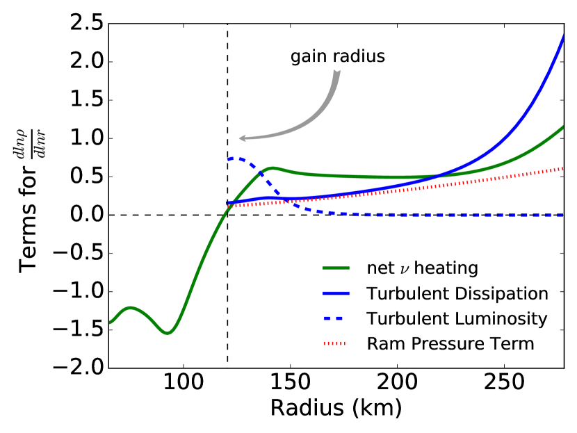
Figure 1: The effects of neutrinos and turbulence on the density and temperature profiles. Specifically, we show the dimensionless terms that appear in the equation for $\frac{d\ln\rho}{d\ln r}$, A1. We omit the pressure and gravity terms which combine to give a power-law slope of about $-3$. Instead we show the net neutrino heating and cooling term (solid-green line) and the effect of each turbulent term. The turbulent dissipation (solid, blue line) and the turbulent luminosity (dashed, blue line) terms originate from the energy equation, and the ram pressure term (dotted, red line) comes from the momentum equation. In our model, we assume that turbulence is driven only in the gain region. In general, the turbulent terms associated with the energy equation are larger than ram pressure. More specifically, turbulent dissipation generally affects the profile more than the ram pressure.

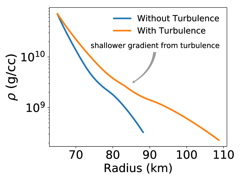
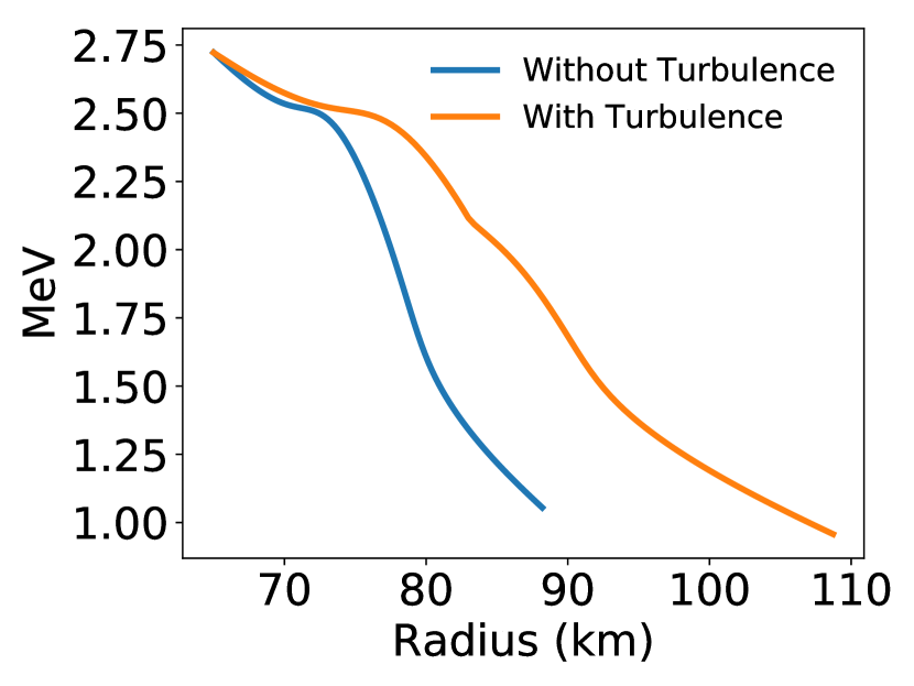
Figure 2: The density and temperature profiles for stalled shock solutions with and without the convection. Generally, convection causes shallower gradients and higher temperatures. While technically all of the terms contribute to this effect, the most dominant term is turbulent dissipation which provides extra heating.

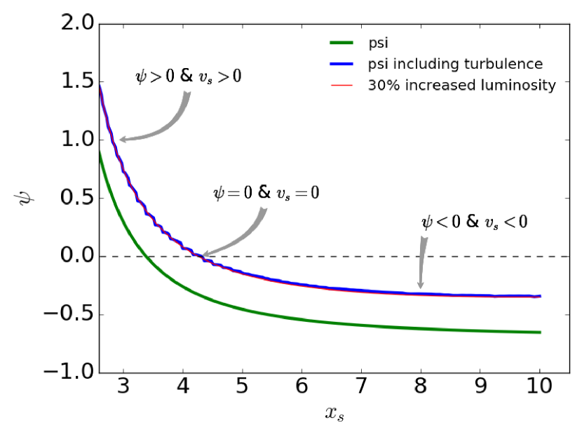
Figure 3: $\Psi$ parameter as a function of shock radius, $x_{s}=R_{s}/R_{\rm NS}$. $\Psi$ is roughly the over pressure compared to hydrostatic equilibrium normalized by the pre-shock ram pressure. The shock velocity is related to $\Psi$ by $v_{s}\approx 1-\sqrt{1+\Psi}$. Therefore, the sign of $\Psi$ determines whether the shock recedes, expands, or is stalled. There is always a minimum for $\Psi$, $\Psi_{\rm min}$. If $\Psi_{\rm min}<0$, then there is always a stalled solution. On the other hand, when $\Psi_{\rm min}>0$, then only $v_{s}>0$ solutions exist. Murphy & Dolence (2017) propose that $\Psi_{\rm min}=0$ is the explosion condition. Adding turbulence has the effect of raising $\Psi_{\rm min}$, making it easier to reach the explosion condition. Adding turbulence has a similar effect as increasing the neutrino luminosity by 30% (red line).

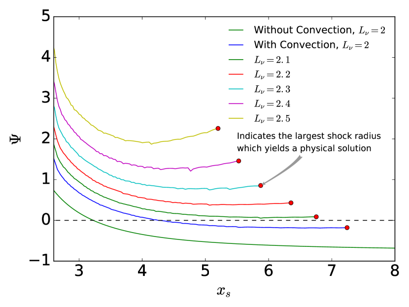
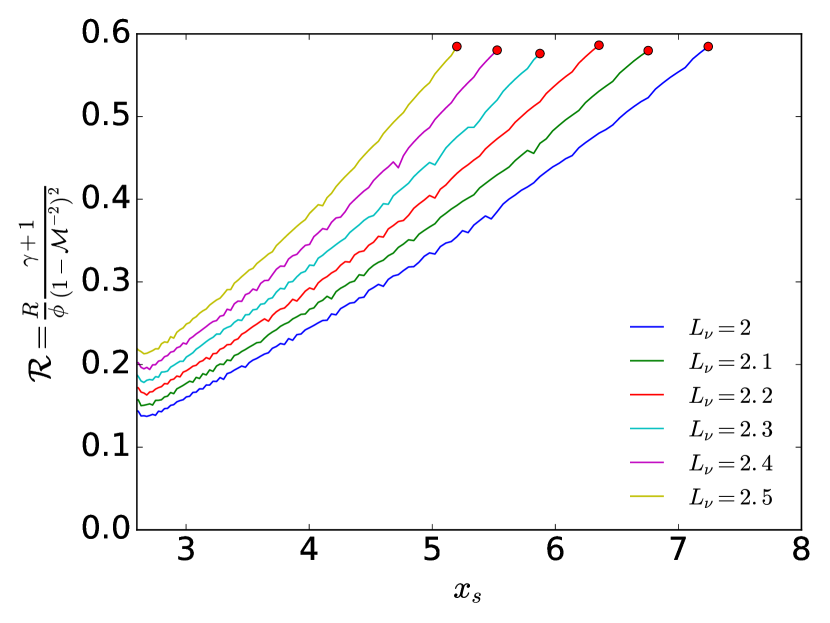
Figure 4: $\Psi$ and corresponding dimensionless Reynolds stress, $\mathcal{R}$, as a function of shock radius ($x_{s}$ = r/$r_{s}$). There is an upper limit for the dimensionless Reynolds stress which we derive in section 2.5 (see equation (40)). Here, we show the behavior of the normalized Reynolds stress vs. $x_{s}$ and how it affects the explodability parameter $\Psi$. In the bottom panel, each $\mathcal{R}$ increases until it reaches an unphysical point and terminates at the red dot. The same termination points can be seen above in the top panel, where each dot corresponds to its respective unphysical shock radius for a given $L_{\nu}$. If the cap had occurred to the left of $\Psi_{\rm min}$ then this upper bound on R would have affected the critical curve. However, the upper limit occurs to the right of $\Psi_{\rm min}$, therefore it does not affect the critical curve. Thus, the critical point of explosion is still dominated by non-ram pressure terms.

Figure 5: How turbulence affects the $\Psi_{\rm min}=0$ explosion condition. $\Psi_{\rm min}$ depends upon five parameters of the core-collapse problem: the neutrino luminosity, $L_{\nu}$, mass accretion rate, $\dot{\mathcal{M}}$, neutron star radius or more specifically the neutrino-sphere radius, $R_{\nu}$, the neutrino temperature, $T_{\nu}$, and the neutron star mass, $M_{\rm NS}$. Therefore, the explosion condition $\Psi_{\rm min}>0$ represents a hypersurface in this five-dimensional parameter space. By fixing 3 of the 5 parameters, one may construct “critical curves” with the other 2 parameters. The critical $L_{\nu}-\dot{\mathcal{M}}$ (lower left panel) is one such example. In each panel, the solid line shows the critical condition $\Psi_{\rm min}=0$, and for all but the top panel explosions occur in the upper portion of the parameter space. The dashed line shows the reduction of the critical condition due to neutrino-driven convection for each critical curve.

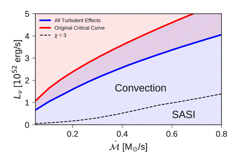
Figure 6: Comparing the relative thresholds of the critical curves and the $\chi=3$ line. Above this line, all stalled solutions have $\chi>3$ (convection dominated), and below this line, $\chi<3$ (SASI dominated). The fact that convection dominates near the critical curve validates our use of a convection-based turbulence model to explore how turbulence affects the critical condition for explosions.

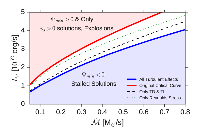
Figure 7: Diagnosing how turbulence affects a critical curve for explosion. Here we show how the various terms affect one particular slice of the $\Psi_{\rm min}=0$ condition, the neutrino-luminosity vs. mass-accretion-rate critical curve. The thick red line is the original critical curve (Burrows & Goshy, 1993), and the thick blue line shows the turbulence induced reduction in the critical curve. The red-shaded region is where $\Psi_{\rm min}>0$ and thus where no steady state solutions exist. The blue-shaded region is the region of stalled shock solutions when including convection. To assess the effects of each of the turbulence terms, we reproduce the critical curve by isolating the turbulent terms in the energy and momentum equations. In the energy equation, the terms are the turbulent dissipation and turbulent luminosity (TD and TL), and in the momentum equation, the only turbulent term is the Reynolds stress (or turbulent ram pressure). The dotted line corresponds to only including Reynolds stress, and the dashed line corresponds to only including the effects of TD and TL. From these results we draw two main conclusions. One, the necessary neutrino energy required for a supernova explosion is less when considering multi-dimensional effects. Two, most of the reduction in the critical condition comes from the energy equation terms, in particular the turbulent dissipation.

Our primary objective is to understand how turbulence affects the conditions for explosion. To fully understand this influence, we also need to understand how turbulence affects the background structure, so we first show how the turbulent terms affects the density and temperature profiles. We then show that turbulence raises the $\Psi$ parameter, implying an easing of the explosion condition. We then consider how this affects the critical hypersurface. To connect to previous investigations, we focus on the neutrino-luminosity and accretion-rate slice of this critical hypersurface. We find that this reduction in the critical curve is $\sim$30%, in concordance with multi-dimensional simulations. To investigate how turbulence reduces the condition for explosion, we calculate the critical condition with each term included and omitted. Lastly, we provide evidence that our upper limit on the Reynolds stress does not affect the actual reduction of the critical curve.

In Figure 1, we illustrate how turbulence affects the density profile; in particular, we show the neutrino and convective terms in the derivative for the density. Since the density profile most closely matches a power-law, we plot terms of d $\ln\rho/$d $\ln r$ to compare how neutrinos and turbulence affect the slope in the log. To reduce the clutter, we do not plot all of the terms; for the full ODE, see equation (A1). In general, the missing terms give a slope that is about -3. In the gain region, both neutrinos and the convective terms make the slope shallower. In the cooling region, neutrino cooling makes the slope steeper. Turbulent dissipation and luminosity terms ultimately originate from the energy equation (3). The turbulent ram pressure term comes from the momentum equation. While turbulent ram pressure does modify the density structure, the two turbulent terms from the energy equation, turbulent dissipation and turbulent luminosity, have a considerably larger effect on the structure.

Figure 2 shows how turbulence affects the density and temperature profiles of the steady-state stalled shock solutions. The net effect of turbulence is to make the profiles much shallower. In part, turbulent ram pressure explains some of the difference, but for the most part, turbulence provides extra heating through dissipation in the convective region. One consequence is that the temperature (and entropy) are higher with turbulence. This is consistent with the entropy profiles of multi-dimensional simulations (Murphy & Meakin, 2011a; Murphy et al., 2013). In agreement with simulations (Murphy et al., 2013; Abdikamalov et al., 2016), Figure 2 also shows that the solution including turbulence has a larger shock radius. The shock radius is a monotonic function of $L_{\nu}$, and since $\rho R_{rr}$ and $\rho\epsilon$ effectively add energy in the same fashion as the luminosity, we intuitively retrieve a larger shock radius. Note that this larger shock radius is not just a consequence of turbulent ram pressure. Instead, the post shock profile is shallower pushing out the shock.

Now that we understand how turbulence affects the density and temperature profiles, we now present how turbulence affects the critical curve in three figures. One, Figure 3 shows how turbulence raises the dimensionless overpressure parameter, $\Psi$, in Murphy & Dolence (2017). Two, Figure 5, shows how turbulence reduces the five-dimensional critical hypersurface for explosion Finally, Figure 7 shows that the dominant turbulent term in reducing the critical condition is turbulent dissipation.

In Figure 3 we plot $\Psi$ to show that the increase in the dimensionless parameter due to turbulence is roughly equivalent to increasing the neutrino luminosity by 30%. To clarify, the $\Psi$ parameter is a measure of the overpressure compared to the hydrostatic equilibrium. This integral condition is normalized by the pre-shock ram pressure. This dimensionless parameter maps directly to the shock velocity in that when $\Psi$ is positive, the shock expands, when $\Psi$ is negative, the shock stalls, and when $\Psi$ = 0, the shock has zero velocity. Note that there is always a minimum $\Psi$, and if this $\Psi_{\rm min}$ is greater than zero, then there are no stalled shock solutions, only steady expanding shocks. For the case where the minimum of $\Psi$ is exactly zero, this set of solutions defines our critical explosion condition for all parameters. Clearly turbulence raises the minimum $\Psi$, and therefore would affect the critical curve.

In figure 4, we show how the Reynolds stress upper limit affects the explodability parameter and the critical curve. We suspected that, at high enough neutrino luminosities, the additional ram pressure at the shock would prevent finding solutions to the boundary conditions. Figure 4 demonstrates that we consistently encounter this cap, but only for pseudo-solutions which have already found a critical $L_{\nu}$. We present several sets of solutions at different neutrino luminosities to emphasize that our $L_{\nu}-\dot{\mathcal{M}}$ critical curve is in fact not affected by the upper limit on $\mathcal{R}$, even at unrealistic luminosities. The sole determination of the critical curve is on $\Psi_{\rm min}=\Psi(r_{\rm s}^{\rm crit})$, and since this threshold is only reached when $r_{\rm s}>r_{\rm s}^{\rm crit}$, there is no effect on the critical curve.

Figure 5 shows how turbulence modifies the critical hypersurface. Murphy & Dolence (2017) points out that the critical condition for explosion is not a critical curve, but a critical hypersurface in a five-dimensional space that is defined by one dimensionless condition: $\Psi_{\rm min}=0$. The neutrino-luminosity-accretion-rate curve is one slice of this critical hypersurface. In Fig. 5, we show six slices of this hypersurface. Note that in all panels except the top-left panel ($M_{\rm NS}$ vs. $\dot{\mathcal{M}}$), the region of explosion is above the curve. For $M_{\rm NS}$ vs. $\dot{\mathcal{M}}$, it is below the curve; a lower mass neutron star has a lower potential to overcome to explode. Because turbulence raises the $\Psi$ curves, it also reduces the critical hypersurface for explosion.

In figure 6, we make a case for the validity of using a convection-based turbulence model. The $\chi$ parameter, first introduced by Foglizzo et al. (2006), is a measure of the linear stability of the convective region in the presence of advection. For $\chi<3$, advection stablizes the flow and convection does not mainfest. The assumption is that since convection is suppressed, the SASI dominates the turublence. The $\chi$ parameter is defined as

$$\chi\equiv\int_{r_{g}}^{r_{s}}\left|\frac{\omega_{buoy}}{u}\right|\,dr$$ (41)

where $\omega_{buoy}$ is the Brunt-Väisälä frequency, defined as

$$\omega^{2}_{buoy}\equiv\left[\frac{1}{p}\left(\frac{\partial p}{\partial S}\right)_{\rho,Y_{e}}\frac{dS}{dr}+\frac{1}{p}\left(\frac{\partial p}{\partial Y_{e}}\right)_{\rho,S}\frac{dY_{e}}{dr}\right]\frac{g}{\Gamma_{1}}\,$$ (42)

and

$$\Gamma_{1}\equiv\left(\frac{\partial\ln P}{\partial\ln\rho}\right)_{S,Y_{e}}\,.$$ (43)

In Figure 6, above the $\chi=3$ dashed line, all stalled solutions have $\chi>3$ (convection dominated) and below this dashed line, all stalled solutions have $\chi<3$ (SASI dominated). To calculate this line, we use a similar approach as deriving the critical luminosity curves: we input all of our parameters, and numerically solve for the luminosity which gives a value of $\chi=3$. According to these models, convection dominates for all scenarios near explosion. Recent simulations seem to support this conclusion (Abdikamalov et al., 2015; Lentz et al., 2015; Couch & O’Connor, 2014; Burrows et al., 2012; Iwakami et al., 2014; Ott et al., 2013; Roberts et al., 2016). The results of Figure 6 validate our exploration of how convection-based turbulence affects the critical condition. However, we do encourage future explorations of the SASI and $\chi$ in simulations to validate wether convection is indeed dominant near the critical condition.

In figures 3 and 5, we considered the overall effect of turbulence on the critical condition, but this does not illuminate how turbulence reduces the condition for explosion. In figure 7, we focus exclusively on the $L_{\nu}-\dot{\mathcal{M}}$ critical curve and explore the effect of each term in this slice of the critical condition. We find that turbulent dissipation within the gain region acts as an even greater driving force for explosion than the turbulent ram pressure. That is not to say that the Reynolds stress is negligible; both terms are indeed needed to obtain the critical curve reduction predicted by multi-dimensional simulations. Though this result relies upon some assumptions in the turbulence model, we suspect that the qualitative outcome will persist: turbulent dissipation can not be dismissed.

3.1 Buoyancy Driven Heating

We argue that turbulent dissipation adds another heat source which aids explosion. Since neutrinos are the ultimate source of energy, it may seem that we are asking neutrinos to do twice the work. However, this is not the case. Using a simple convective model, we propose that in one dimension, some of the neutrino energy goes into heating the material, and some of it goes into creating a higher potential profile. In multiple dimensions, this higher potential profile is unstable, goes to a lower potential profile, and the excess energy goes into kinetic energy, which in turn dissipates as heat via turbulent dissipation.

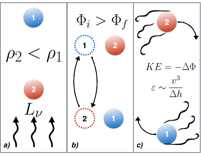
Figure 8: Neutrinos heat the gain region and setup a higher potential state, which turbulence taps and dissipates as heat. Panel a): when a parcel of matter advects through the gain region, neutrinos heat it, which sets up a buoyantly unstable situation. Panel b): Parcel 1 wants to buoyantly sink and parcel 2 wants to buoyantly rise. The final state has a lower potential energy than the final state. Panel c): This change in potential energy is converted to turbulent kinetic energy which dissipates via turbulent dissipation. Therefore, in 1D, part of the energy of neutrinos heats the gain region and part of the neutrino energy goes into setting up the higher potential profile. Multi-dimensional turbulence taps into this higher potential energy by allowing for a lower potential state and turbulent kinetic energy. Then that turbulent kinetic energy is dissipated through viscosity.

Rayleigh-Bénard convection is a simple convective model which can clearly demonstrate this conversion from potential to kinetic to dissipated internal energy. Figure 8 illustrates the fundamental physics of convection. First, neutrinos provide a source of heating and drives a convective instability. In this cartoon model, we consider two parcels; the lower one receives more neutrino heating, has a higher entropy, and lower density compared to its surroundings. The parcel at a higher height has a lower entropy and higher density compared to its surroundings. If one switches the positions of these two parcels, then one finds that the gravitational potential is lower. Therefore, neutrino heating causes a higher potential structure that is unstable to convective overturn. The difference in potentials between the two states gets converted into kinetic energy of the parcels. Kolmogorov’s hypothesis suggests that the dissipation of this kinetic energy is $R^{3/2}/\mathcal{L}$ and happens on the order of one turnover timescale. Burrows et al. (1995) also considered this idea in which two layers of varying densities are swapped, inducing a buoyant work being done on the system. This energy is then converted into kinetic energy in the form of eddies, and in turn dissipated into heat. Therefore, not only do neutrinos heat the gain region, but they also create a higher potential system. This higher potential gets converted to kinetic energy and consequently dissipated as internal energy.

To illustrate this more clearly, consider the energy equation (3). It is more illuminating if we rewrite the equation considering a constant mass accretion rate:

$$\dot{\mathcal{M}}\partial_{i}\left[h+\frac{u^{j}u_{j}}{2}-\Phi\right]=\rho q$$ (44)

Neutrinos heat the convective region of the star, changing the enthalpy and gravitational potential. This gives rise to an entropy and density gradient such that $S_{2}>S_{1}$ and $\rho_{2}<\rho_{1}$ (thus satisfying the Schwarzschild condition for convection). We then treat the potential energy of two parcels in a similar manner to Burrows et al. (1995). Before the exchange of parcels, the gravitational potential energy is

$$\Phi_{1}=gV(\rho_{1}h_{1}+\rho_{2}h_{2})$$ (45)

But after the top parcel sinks and the bottom parcel buoyantly rises, the potential is then

$$\Phi_{2}=gV(\rho_{2}h_{1}+\rho_{1}h_{2})$$ (46)

Thus, the change in potential is

$$\Delta\Phi=gV(\rho_{2}-\rho_{1})(h_{1}-h_{2})$$ (47)

Since $h_{1}>h_{2}$ and $\rho_{1}>\rho_{2}$, $\Delta\Phi<0$. Conservation of energy suggests that K.E.$\approx$-$\Delta\Phi$, and via turbulent dissipation, this energy from buoyant driving is converted into heat. In summary, neutrinos heat the gain region and setup a higher potential profile. Turbulence allows a lower potential state and the kinetic energy is converted into thermal energy via turbulent dissipation, aiding explosion.

4 Conclusion

A major result of core-collapse theory is that one-dimensional simulations fizzle for all but the least massive stars, while multi-dimensional simulations explode for the most part. Even though there are still some differences between the simulations, there is a general consensus that turbulence makes the difference between a fizzled outcome and a successful explosion. To explain how turbulence aids explosion, we develop a turbulence model for neutrino-driven convection (Murphy et al., 2013) and investigate how turbulence reduces the critical condition for explosion (Burrows & Goshy, 1993; Murphy & Dolence, 2017). Our turbulence model reduces the critical condition for explosion by $\sim$30%, in general agreement with simulations. By modeling each turbulent term, we are able to investigate the effect of each turbulent term on the critical condition. We find that although ram pressure plays a role in reducing the critical curve, it is not the dominant term. The dominant term in reducing the critical curve is turbulent dissipation. Furthermore, we are not the first to suggest that turbulent dissipation is important in aiding neutrino-driven explosions. Thompson et al. (2005) suggested that MRI driven turbulence for very rapidly rotating proto-neutron stars could add significant heating and aid explosion.

In the turbulence model, we include all turbulent terms, both in the background solution and in the boundary conditions. The three main turbulent terms are turbulent dissipation, Reynolds stress, and turbulent luminosity. Overall, we find that all three play an important role in modifying the background structure and the critical condition for explosion. However, it is the terms in the energy equation, the combined turbulent luminosity and turbulent dissipation, which give the largest reduction in the critical curve. Of these two, the turbulent dissipation provides the largest effect in reducing the critical condition.

The ultimate source of power for convection and turbulent dissipation is the neutrino driving power. This may seem as if we are double counting the power supplied by neutrinos. However, we are not. Instead, we propose that neutrinos heat the gain region and setup a higher potential, convectively unstable structure. In multi-dimensional simulations, convection converts this higher potential structure to a lower potential structure. The change in potential energy is converted to kinetic turbulent energy, which in turn dissipates as heat. We suggest that CCSN modelers check the structures of their one-dimensional and multi-dimensional simulations to test this supposition.

The turbulence model is a global, integral model, and provides little constraint on the local structure of turbulence, but a local model is necessary in solving the background equations and deriving a critical condition. Therefore, we made some fairly straightforward assumptions to translate the global model to a local model. For example, we assumed that the specific turbulent dissipation rate is constant throughout the gain region. We also had to assume a specific spatial profile for the turbulent luminosity. These assumptions probably do not affect our qualitative results. However, our results have large implications regarding how turbulence aids explosion. In particular, we propose that turbulent dissipation is a key contributor to reviving a stalled shock to a successful supernova. Therefore, these assumptions shoud be verified with multi-dimensional simulations and treated more rigorously in future investigations.

To verify the predictions of this manuscript, we identify at least three open questions that multi-dimensional simulations should address. One, does turbulent dissipation actually lead to significant heating? In multiple dimensions, the entropy profile should be a result of neutrino heating and cooling, turbulent entropy flux, and turbulent dissipation. One can easily calculate the turbulent entropy flux, and the heating and cooling by neutrinos. What ever is left should be equal to the expected entropy generated by turbulent dissipation. Second, do the one-dimensional profiles have a higher potential compared to their multi-dimensional counterparts? Third, do the local details of the turbulent model matter? We suspect that the local details do not change the qualitative result. However, one should compare our local assumptions with multi-dimensional simulations, and assess how (if at all) the quantitative results vary from this work.

In summary, combining a turbulence model and critical condition analyses helps to illuminate how turbulence aids explosions. Specifically, by modeling each turbulent term we are able to assess the effect of each term in the conditions for explosion. Contrary to prior suppositions, we find that turbulent ram pressure is not the dominant effect. Rather, each of the three terms are quite large in their effect with turbulent dissipation being the largest. Presently, these conclusions are qualitative. To be predictive, the community will need to verify these conclusions with multi-dimensional simulations. Eventually, we may be able to use these turbulence models to make one-dimensional simulations explode under similar conditions as multi-dimensional simulations, thereby enabling rapid and systematic exploration of the explosion of massive stars.

Appendix A Full ODEs

Here, we present the full set of ordinary differential equations that we solve to find pseudo steady-state solutions. The equation for density is

$$\scalebox{1.3}{$\frac{dln\rho}{dlnr}=\frac{\frac{2v^{2}}{\Phi}-1+\mathcal{RS}+\frac{y}{l}\frac{\frac{\partial lny}{\partial lnT}}{\frac{\partial lnl}{\partial lnT}}\big{(}1+\mathcal{H}-\mathcal{C}+\mathcal{TD}-\mathcal{TL}+\frac{2v^{2}}{\Phi}\big{)}}{y-\frac{v^{2}}{\Phi}+y\frac{\partial lny}{\partial ln\rho}+\frac{\frac{\partial lny}{\partial lnT}}{\frac{\partial lnl}{\partial lnT}}\big{(}\frac{yv^{2}}{\Phi l}-\frac{\partial lnl}{\partial ln\rho}\big{)}}$}\,,$$ (A1)

and in terms of the density equation, the temperature ODE is

$$\scalebox{1.3}{$\frac{\partial\ln T}{\partial\ln r}=\frac{\big{(}1+\mathcal{H}-\mathcal{C}+\mathcal{TD}-\mathcal{TL}+\frac{2v^{2}}{\Phi}\big{)}}{l\frac{\partial lnl}{\partial lnT}}+\frac{\frac{\partial ln\rho}{\partial lnr}}{\frac{\partial lnl}{\partial lnT}}\bigg{(}\frac{v^{2}}{\Phi l}-\frac{\partial lnl}{\partial ln\rho}\bigg{)}$}\,.$$ (A2)

In this form, these equations seem some what unwieldy, but they would be even more so if we had not made the following shorthand for the important physics. To further help illustrate the important scales in the problem, we present each important physics in terms of a dimensionless variable. The Reynolds stress (or ram pressure) appears in the above equations as

$$\mathcal{RS}=\frac{2x^{2}R_{rr}}{(x_{s}-x_{g})\Phi_{1}}\,.$$ (A3)

In these expressions, the subscript 1 indicates the base of the solution. In our particular case, that is the neutrino-sphere radius. Neutrino heating and cooling are

$$\mathcal{H}=\frac{L_{\nu}\kappa\rho r_{1}x^{2}}{\dot{\mathcal{M}}\Phi_{1}}\,,$$ (A4)

and

$$\mathcal{C}=\frac{C_{0}\big{(}\frac{T}{T_{0}}\big{)}^{6}4\pi r_{1}^{3}x^{4}\rho}{\dot{\mathcal{M}}\Phi_{1}}\,.$$ (A5)

The two turbulent terms from the energy equation are the turbulent dissipation and turbulent luminosity:

$$\mathcal{TD}=\frac{L_{e}^{max}r_{1}^{3}\rho w_{b}4\pi}{M_{g}\dot{\mathcal{M}}\Phi_{1}}$$ (A6)

and

$$\mathcal{TL}=\frac{L_{e}^{max}r_{1}x^{2}}{cosh^{2}\big{(}\frac{(r_{1}(x-x_{g}))}{h}\big{)}h\dot{\mathcal{M}}\Phi_{1}}\,.$$ (A7)

Two dimensionless measures of the pressure and enthalpy are

$$y=\frac{P}{\rho\Phi}$$ (A8)

and

$$l=\frac{e+\frac{P}{\rho}}{\Phi}$$ (A9)

$$P_{,\rho}=\frac{\partial\ln P}{\partial\ln\rho}\bigg{|}_{T}$$ (A10)

The normalized radius is

$$x=\frac{r}{r_{NS}}\,.$$ (A11)

A dimensionless measure of the bouyant driving is

$$w_{b}=\int\limits_{x_{g}}^{x_{s}}\frac{tanh\big{(}\frac{r_{1}(x-x_{g})}{h}\big{)}}{3yx}dx\,.$$ (A12)

To observe and distinguish the effects of each turbulent term, we add the capability to turn each term on or off in the equations. In doing so, we investigate the effect of each term on the solutions and critical curves.

References

- Abdikamalov et al. (2016) Abdikamalov, E., Zhaksylykov, A., Radice, D., & Berdibek, S. 2016, ArXiv e-prints, arXiv:1605.09015
- Abdikamalov et al. (2015) Abdikamalov, E., Ott, C. D., Radice, D., et al. 2015, ApJ, 808, 70
- Armstrong et al. (1995) Armstrong, J. W., Rickett, B. J., & Spangler, S. R. 1995, ApJ, 443, 209
- Bethe (1990) Bethe, H. A. 1990, Reviews of Modern Physics, 62, 801
- Bethe & Wilson (1985) Bethe, H. A., & Wilson, J. R. 1985, ApJ, 295, 14
- Blondin et al. (2003) Blondin, J. M., Mezzacappa, A., & DeMarino, C. 2003, ApJ, 584, 971
- Bruenn et al. (2016) Bruenn, S. W., Lentz, E. J., Hix, W. R., et al. 2016, ApJ, 818, 123
- Buras et al. (2006a) Buras, R., Janka, H.-T., Rampp, M., & Kifonidis, K. 2006a, A&A, 457, 281
- Buras et al. (2006b) —. 2006b, A&A, 457, 281
- Buras et al. (2003) Buras, R., Rampp, M., Janka, H.-T., & Kifonidis, K. 2003, Physical Review Letters, 90, 241101
- Burrows et al. (2007) Burrows, A., Dessart, L., Ott, C. D., & Livne, E. 2007, Phys. Rep., 442, 23
- Burrows et al. (2012) Burrows, A., Dolence, J. C., & Murphy, J. W. 2012, ApJ, 759, 5
- Burrows & Goshy (1993) Burrows, A., & Goshy, J. 1993, ApJ, 416, L75
- Burrows et al. (1995) Burrows, A., Hayes, J., & Fryxell, B. A. 1995, ApJ, 450, 830
- Burrows et al. (2016) Burrows, A., Vartanyan, D., Dolence, J. C., Skinner, M. A., & Radice, D. 2016, ArXiv e-prints, arXiv:1611.05859
- Canuto (1993) Canuto, V. M. 1993, ApJ, 416, 331
- Colgate & Herant (2004) Colgate, S. A., & Herant, M. E. 2004, in Cosmic explosions in three dimensions, ed. P. Höflich, P. Kumar, & J. C. Wheeler, 199
- Couch (2013) Couch, S. M. 2013, ApJ, 775, 35
- Couch & O’Connor (2014) Couch, S. M., & O’Connor, E. P. 2014, ApJ, 785, 123
- Couch & Ott (2015) Couch, S. M., & Ott, C. D. 2015, ApJ, 799, 5
- Dolence et al. (2013) Dolence, J. C., Burrows, A., Murphy, J. W., & Nordhaus, J. 2013, ApJ, 765, 110
- Dolence et al. (2015) Dolence, J. C., Burrows, A., & Zhang, W. 2015, ApJ, 800, 10
- Ertl et al. (2016) Ertl, T., Janka, H.-T., Woosley, S. E., Sukhbold, T., & Ugliano, M. 2016, ApJ, 818, 124
- Fernández (2015a) Fernández, R. 2015a, MNRAS, 452, 2071
- Fernández (2015b) —. 2015b, MNRAS, 452, 2071
- Fernández et al. (2014) Fernández, R., Müller, B., Foglizzo, T., & Janka, H.-T. 2014, MNRAS, 440, 2763
- Foglizzo et al. (2006) Foglizzo, T., Scheck, L., & Janka, H.-T. 2006, ApJ, 652, 1436
- Foglizzo & Tagger (2000) Foglizzo, T., & Tagger, M. 2000, A&A, 363, 174
- Foglizzo et al. (2015) Foglizzo, T., Kazeroni, R., Guilet, J., et al. 2015, PASA, 32, e009
- Guilet et al. (2010) Guilet, J., Sato, J., & Foglizzo, T. 2010, ApJ, 713, 1350
- Handy et al. (2014) Handy, T., Plewa, T., & Odrzywołek, A. 2014, ApJ, 783, 125
- Hanke et al. (2012) Hanke, F., Marek, A., Müller, B., & Janka, H.-T. 2012, ApJ, 755, 138
- Hanke et al. (2013) Hanke, F., Müller, B., Wongwathanarat, A., Marek, A., & Janka, H.-T. 2013, ApJ, 770, 66
- Herant et al. (1994) Herant, M., Benz, W., Hix, W. R., Fryer, C. L., & Colgate, S. A. 1994, ApJ, 435, 339
- Hillebrandt & Mueller (1981) Hillebrandt, W., & Mueller, E. 1981, A&A, 103, 147
- Horiuchi et al. (2011) Horiuchi, S., Beacom, J. F., Kochanek, C. S., et al. 2011, ApJ, 738, 154
- Iwakami et al. (2014) Iwakami, W., Nagakura, H., & Yamada, S. 2014, ApJ, 793, 5
- Janka (2001) Janka, H.-T. 2001, A&A, 368, 527
- Janka (2017) —. 2017, ArXiv e-prints, arXiv:1702.08825
- Janka & Keil (1998) Janka, H.-T., & Keil, W. 1998, in Supernovae and cosmology, ed. L. Labhardt, B. Binggeli, & R. Buser, 7
- Janka et al. (2016) Janka, H.-T., Melson, T., & Summa, A. 2016, ArXiv e-prints, arXiv:1602.05576
- Janka & Müller (1995) Janka, H.-T., & Müller, E. 1995, ApJ, 448, L109
- Janka & Müller (1996) —. 1996, A&A, 306, 167
- Kitaura et al. (2006) Kitaura, F. S., Janka, H.-T., & Hillebrandt, W. 2006, A&A, 450, 345
- Kolmogorov (1941) Kolmogorov, A. 1941, Akademiia Nauk SSSR Doklady, 30, 301
- Lentz et al. (2015) Lentz, E. J., Bruenn, S. W., Hix, W. R., et al. 2015, ArXiv e-prints, arXiv:1505.05110
- Li et al. (2011) Li, W., Leaman, J., Chornock, R., et al. 2011, MNRAS, 412, 1441
- Liebendörfer et al. (2001a) Liebendörfer, M., Mezzacappa, A., & Thielemann, F.-K. 2001a, Phys. Rev. D, 63, 104003
- Liebendörfer et al. (2001b) Liebendörfer, M., Mezzacappa, A., Thielemann, F.-K., et al. 2001b, Phys. Rev. D, 63, 103004
- Liebendörfer et al. (2005) Liebendörfer, M., Rampp, M., Janka, H.-T., & Mezzacappa, A. 2005, ApJ, 620, 840
- Marek & Janka (2009) Marek, A., & Janka, H.-T. 2009, ApJ, 694, 664
- Mazurek (1982) Mazurek, T. J. 1982, ApJ, 259, L13
- Mazurek et al. (1982) Mazurek, T. J., Cooperstein, J., & Kahana, S. 1982, in NATO Advanced Science Institutes (ASI) Series C, Vol. 90, NATO Advanced Science Institutes (ASI) Series C, ed. M. J. Rees & R. J. Stoneham, 71–77
- Meakin & Arnett (2007) Meakin, C. A., & Arnett, D. 2007, ApJ, 667, 448
- Meakin & Arnett (2010) Meakin, C. A., & Arnett, W. D. 2010, Ap&SS, 328, 221
- Melson et al. (2015) Melson, T., Janka, H.-T., & Marek, A. 2015, ApJ, 801, L24
- Müller (2016) Müller, B. 2016, ArXiv e-prints, arXiv:1608.03274
- Müller (2017) —. 2017, ArXiv e-prints, arXiv:1702.06940
- Müller et al. (2016) Müller, B., Heger, A., Liptai, D., & Cameron, J. B. 2016, MNRAS, 460, 742
- Müller et al. (2017) Müller, B., Melson, T., Heger, A., & Janka, H.-T. 2017, ArXiv e-prints, arXiv:1705.00620
- Murphy & Burrows (2008) Murphy, J. W., & Burrows, A. 2008, ApJ, 688, 1159
- Murphy & Dolence (2017) Murphy, J. W., & Dolence, J. C. 2017, ApJ, 834, 183
- Murphy et al. (2013) Murphy, J. W., Dolence, J. C., & Burrows, A. 2013, ApJ, 771, 52
- Murphy & Meakin (2011a) Murphy, J. W., & Meakin, C. 2011a, ApJ, 742, 74
- Murphy & Meakin (2011b) —. 2011b, ApJ, 742, 74
- O’Connor & Ott (2011) O’Connor, E., & Ott, C. D. 2011, ApJ, 730, 70
- Ott et al. (2013) Ott, C. D., Abdikamalov, E., Mösta, P., et al. 2013, ApJ, 768, 115
- Pejcha & Thompson (2012) Pejcha, O., & Thompson, T. A. 2012, ApJ, 746, 106
- Radice et al. (2017) Radice, D., Burrows, A., Vartanyan, D., Skinner, M. A., & Dolence, J. C. 2017, ArXiv e-prints, arXiv:1702.03927
- Radice et al. (2016) Radice, D., Ott, C. D., Abdikamalov, E., et al. 2016, ApJ, 820, 76
- Rampp & Janka (2002) Rampp, M., & Janka, H.-T. 2002, A&A, 396, 361
- Roberts et al. (2016) Roberts, L. F., Ott, C. D., Haas, R., et al. 2016, ArXiv e-prints, arXiv:1604.07848
- Sato et al. (2009a) Sato, J., Foglizzo, T., & Fromang, S. 2009a, ApJ, 694, 833
- Sato et al. (2009b) Sato, J., Foglizzo, T., & Fromang, S. 2009b, in SF2A-2009: Proceedings of the Annual meeting of the French Society of Astronomy and Astrophysics, ed. M. Heydari-Malayeri, C. Reyl’E, & R. Samadi, 175
- Tamborra et al. (2017) Tamborra, I., Hüdepohl, L., Raffelt, G. G., & Janka, H.-T. 2017, ApJ, 839, 132
- Thompson (2000) Thompson, C. 2000, ApJ, 534, 915
- Thompson et al. (2003) Thompson, T. A., Burrows, A., & Pinto, P. A. 2003, ApJ, 592, 434
- Thompson et al. (2005) Thompson, T. A., Quataert, E., & Burrows, A. 2005, ApJ, 620, 861
- Yamasaki & Yamada (2005) Yamasaki, T., & Yamada, S. 2005, ApJ, 623, 1000
- Yamasaki & Yamada (2006) —. 2006, ApJ, 650, 291