Biased Importance Sampling for Deep Neural Network Training

Abstract

Importance sampling has been successfully used to accelerate stochastic optimization in many convex problems. However, the lack of an efficient way to calculate the importance still hinders its application to Deep Learning.

In this paper, we show that the loss value can be used as an alternative importance metric, and propose a way to efficiently approximate it for a deep model, using a small model trained for that purpose in parallel.

This method allows in particular to utilize a biased gradient estimate that implicitly optimizes a soft max-loss, and leads to better generalization performance. While such method suffers from a prohibitively high variance of the gradient estimate when using a standard stochastic optimizer, we show that when it is combined with our sampling mechanism, it results in a reliable procedure.

We showcase the generality of our method by testing it on both image classification and language modeling tasks using deep convolutional and recurrent neural networks. In particular, our method results in 30% faster training of a CNN for CIFAR10 than when using uniform sampling.

Introduction

The dramatic increase in available training data has made the use of Deep Neural Networks feasible, which in turn has significantly improved the state-of-the-art in many fields, in particular Computer Vision and Natural Language Processing. However, due to the complexity of the resulting optimization problem, computational cost is now the core issue in training these large architectures.

When training such models, it appears to any practitioner that not all samples are equally important; many of them are properly handled after a few epochs of training, and most could be ignored at that point without impacting the final model. To this end, we propose a novel importance sampling scheme that accelerates the training, in theory, of any Neural Network architecture.

For convex optimization problems, many works (?; ?; ?; ?; ?) have taken advantage of the difference in importance among the samples to improve the convergence speed of stochastic optimization methods. However, only recently, researchers (?; ?) have shifted their focus on using importance sampling for training Deep Neural Networks. Compared to these works, we propose an importance sampling scheme based on the loss and show that our method can be used to improve the convergence of various architectures on realistic text and image datasets, while at the same time using a minimal number of hyperparameters.

? ̵̃(?) prove that sampling with a distribution proportional to the gradient norm of each sample, is optimal in minimizing the variance of the gradients; thus resulting in a convergence speed-up for Stochastic Gradient Descent (SGD). However, using the gradient norm requires computing second-order quantities during the backward pass, which is computationally prohibitive. We show, theoretically, that using the loss, we can construct an upper bound to the gradient norm that is better than uniform. Nevertheless, computing the loss still requires a full forward pass, hence using it directly on all the samples remains intractable. In order to reduce the computational cost even more, we propose to use the prediction of a small network, trained alongside the deep model we want to eventually train, to predict an approximation of the importance of the training samples. The complexity of this surrogate allows us to modulate the cost / accuracy trade-off.

Finally, we also show a relationship between importance sampling and maximum-loss minimization, which can be used to improve the generalization ability of the trained Deep Neural Network.

In summary, the contributions of this work are:

• We show that using the loss, we can construct a sampling distribution that reduces the variance of the gradients compared to uniform sampling

• The creation of a model able to approximate the loss for a low computational overhead

• The development of an online algorithm that minimizes a soft max-loss in the training set through importance sampling

Related Work

Importance sampling for convex problems has received significant attention over the years. ? ̵̃(?) developed LASVM, which is an online algorithm that uses importance sampling to train kernelized support vector machines. Later ? ̵̃(?) and more recently ? ̵̃(?) developed more general importance sampling methods that improve the convergence of Stochastic Gradient Descent. In particular, the latter has crucially connected the convergence speed of SGD with the variance of the gradient estimator and has shown that the target sampling distribution is the one that minimizes this variance.

? ̵̃(?) are the first ones, to our knowledge, that attempted to use importance sampling for training Deep Neural Networks. They sample according to the exact gradient norm as computed by a cluster of GPU workers. Even with a cluster of GPUs they have to constrain the networks that they use to fully connected layers in order to be able to compute the gradient norm in a reasonable time. Compared to their approach, the proposed method achieves wall-clock time speed-up, for any architecture, requiring the same resources as plain uniform sampling.

? ̵̃(?) looked towards the loss value to build a sampling distribution for mini-batch creation for Deep Neural Networks. Their method provides the Neural Network with samples that have been previously seen to have high loss. The most important limitation of their work is the introduction of several hard to choose hyperparameters that also impede the generalization of their method to datasets other than MNIST. On the other hand, we conduct experiments with more challenging image and text datasets and show that our method generalizes well without the need to choose any hyperparameters.

? ̵̃(?) worked on improving the sampling procedure for importance sampling. They imposed a prior tree structure on the weights, and use a sampling procedure inspired by the Monte Carlo Tree Search algorithm, that handles properly the exploration / exploitation dilemma and converges asymptotically to the probability distribution of the weights. However, this method fully relies on the existence of the tree structure, that should reflect the regularity of the importance on the samples, which is in itself a quite complicated embedding problem.

Finally, there is another class of methods related to importance sampling that can be perceived as using an importance metric quite antithetical to most common methods. Curriculum learning (?) and its evolution self-paced learning (?) present the classifier with easy samples first (samples that are likely to have a small loss) and gradually introduce harder and harder samples.

Importance Sampling

Importance sampling aims at increasing the convergence speed of SGD by reducing the variance of the gradient estimates. In the following sections, we analyze how this works and present an efficient procedure that can be used to train any Deep Learning model. Moreover, we also show that our importance sampling method has a close relation to maximum loss minimization, which can result in improved generalization performance.

Exact Importance Sampling

Let $x_{i}$, $y_{i}$ be the $i$-th input-output pair from the training set, $\Psi(\cdot;\theta)$ a Deep Learning model parameterized by the vector $\theta$, and $L(\cdot,\cdot)$ the loss function to be minimized during training. The goal of training is to find

$$\theta^{*}=\operatorname*{arg\,min}_{\theta}\frac{1}{N}\sum_{i=1}^{N}L(\Psi(x_{i};\theta),y_{i})$$ (1)

where $N$ corresponds to the number of examples in the training set. Using Stochastic Gradient Descent with learning rate $\eta$, we iteratively update the parameters of our model, between two consecutive iterations $t$ and $t+1$, with

$$\theta_{t+1}=\theta_{t}-\eta\alpha_{i}\nabla_{\theta_{t}}L(\Psi(x_{i};\theta_{t}),y_{i})$$ (2)

where $i$ is a discrete random variable sampled according to a distribution $P$ with probabilities $p_{i}$ and $\alpha_{i}$ is a sample weight. For instance, plain SGD with uniform sampling is achieved with $\alpha_{i}=1$ and $p_{i}=\frac{1}{N}$ for all $i$.

If we define the convergence speed $S$ of SGD as the reduction of the distance of the parameter vector $\theta$ from the optimal parameter vector $\theta^{*}$ in two consecutive iterations $t$ and $t+1$

$$S=-\operatorname{\mathbb{E}}_{P}\left[\left\lVert\theta_{t+1}-\theta^{*}\right\rVert_{2}^{2}-\left\lVert\theta_{t}-\theta^{*}\right\rVert_{2}^{2}\right],$$ (3)

and if we have

$$\operatorname{\mathbb{E}}_{P}\left[\alpha_{i}\nabla_{\theta_{t}}L(\Psi(x_{i};\theta_{t}),y_{i})\right]=\nabla_{\theta_{t}}\frac{1}{N}\sum_{i=1}^{N}L(\Psi(x_{i};\theta_{t}),y_{i}),$$ (4)

and set $G_{i}=\alpha_{i}\nabla_{\theta_{t}}L(\Psi(x_{i};\theta_{t}),y_{i})$, then we get (this is a different derivation of the result by ? ̵̃(?))

$$S =-\operatorname{\mathbb{E}}_{P}\left[\left(\theta_{t+1}-\theta^{*}\right)^{T}\left(\theta_{t+1}-\theta^{*}\right)-\left(\theta_{t}-\theta^{*}\right)^{T}\left(\theta_{t}-\theta^{*}\right)\right]$$ (5)

$$=-\operatorname{\mathbb{E}}_{P}\left[\theta_{t+1}^{T}\theta_{t+1}-2\theta_{t+1}\theta^{*}-\theta_{t}^{T}\theta_{t}+2\theta_{t}\theta^{*}\right]$$

$$=-\operatorname{\mathbb{E}}_{P}\left[\left(\theta_{t}-\eta G_{i}\right)^{T}\left(\theta_{t}-\eta G_{i}\right)+2\eta G_{i}^{T}\theta^{*}-\theta_{t}^{T}\theta_{t}\right]$$

$$=-\operatorname{\mathbb{E}}_{P}\left[-2\eta\left(\theta_{t}-\theta^{*}\right)G_{i}+\eta^{2}G_{i}^{T}G_{i}\right]$$

$$=2\eta\left(\theta_{t}-\theta^{*}\right)\operatorname{\mathbb{E}}_{P}\left[G_{i}\right]-\eta^{2}\operatorname{\mathbb{E}}_{P}\left[G_{i}\right]^{T}\operatorname{\mathbb{E}}_{P}\left[G_{i}\right]-$$

$$\quad\,\eta^{2}\text{Tr}\left(\operatorname{\mathbb{V}}_{P}\left[G_{i}\right]\right)$$

From the last expression, we observe that it is possible to gain a speedup by sampling from the distribution that minimizes $\text{Tr}\left(\operatorname{\mathbb{V}}_{P}\left[G_{i}\right]\right)$. ? ̵̃(?) and ? ̵̃(?) show that this distribution has probabilities $p_{i}\propto\left\lVert\nabla_{\theta_{t}}L(\Psi(x_{i};\theta_{t}),y_{i})\right\rVert_{2}$. However, computing the norm of the gradient for each sample is computationally intensive. ? ̵̃(?) use a distributed cluster of workers and constrain their models to fully connected networks while ? ̵̃(?) only consider convex problems and sample according to the Lipschitz constant of the loss of each sample, which is an upper bound of the gradient norm.

To mitigate the computational requirement, we propose to use the loss itself as the importance metric instead of the gradient norm. Although providing the network with a larger number of confusing examples makes intuitive sense, we show that the loss can be used to create a tighter upper bound to the gradient norm than plain uniform sampling using the following theorem.

Theorem 1.

Let $G_{i}=\left\lVert\nabla_{\theta_{t}}L(\Psi(x_{i};\theta_{t}),y_{i})\right\rVert$ and $M=\max G_{i}$. There exist $K>0$ and $C<M$ such that

$$\frac{1}{K}L(\Psi(x_{i};\theta_{t}),y_{i})+C\geq G_{i}\quad\forall i$$ (6)

The above theorem is derived using the fact that the ordering of samples according to the loss is reflected by their ordering according to the gradient norm. A complete proof of the theorem is provided in the supplementary material. Despite the fact that theorem 2 only proves that sampling using the loss is an improvement compared to uniform sampling, in our experiments we show that it exhibits similar variance reducing properties to sampling according to the gradient norm thus resulting in convergence speed improvement compared to uniform sampling.

To sum up, we propose the following importance sampling scheme that creates an unbiased estimator of the gradient vector of Batch Gradient Descent with lower variance:

$$p_{i} \propto L(\Psi(x_{i};\theta_{t}),y_{i})$$ (7)

$$\alpha_{i} =\frac{1}{Np_{i}}.$$ (8)

Relation to Max Loss Minimization

Minimizing the average loss over the training set does not necessarily result in the best model for classification. ? ̵̃(?) argue that minimizing the maximum loss can lead to better generalization performance, especially if there exist a few “rare” samples in the training set. In this section, we show that introducing a minor bias inducing modification in the sample weights $\alpha_{i}$, we are able to focus on the high-loss samples with a variable intensity up to the point of minimizing the maximum loss.

Instead of choosing the sample weights $\alpha_{i}$ such that we get an unbiased estimator of the gradient, we define them according to

$$\alpha_{i}=\frac{1}{Np_{i}^{k}},\ \text{with}\ k\in(-\infty,1].$$ (9)

Using $L_{i}=L(\Psi(x_{i};\theta),y_{i})$ and $p_{i}\propto L_{i}$, we get

$$\operatorname{\mathbb{E}}_{P}\left[\alpha_{i}\nabla_{\theta}L_{i}\right] =\sum_{i=1}^{N}p_{i}\alpha_{i}\nabla_{\theta}L_{i}$$ (10)

$$=\sum_{i=1}^{N}\frac{p_{i}^{1-k}}{N}\nabla_{\theta}L_{i}$$ (11)

$$\propto\sum_{i=1}^{N}\frac{L_{i}^{1-k}}{N}\nabla_{\theta}L_{i}$$ (12)

$$\propto\sum_{i=1}^{N}\frac{1}{N}\nabla_{\theta}L_{i}^{2-k},$$ (13)

which is an unbiased estimator of the gradient of the original loss function raised to the power $2-k\geq 1$. When $2-k\gg 1$ we essentially minimize the maximum loss but as it will be analyzed in the experiments, smaller values can be helpful both in increasing the convergence speed and improving the generalization error.

Approximate Importance Sampling

 

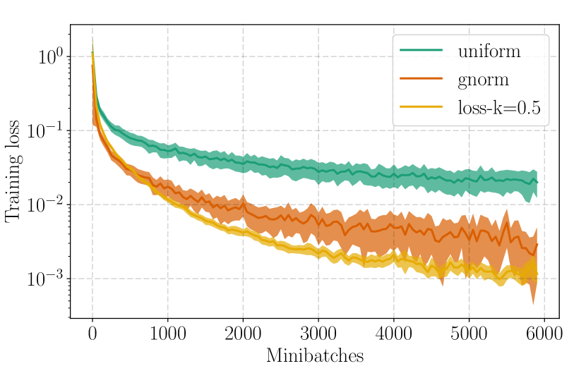
(a) Variance reduction

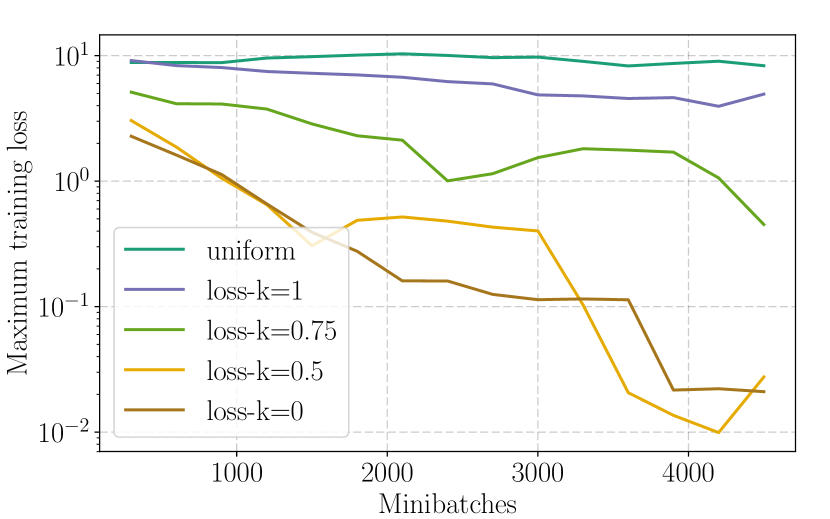
(b) Effect of $k$

Figure 1: Averaged results of $10$ independent runs on MNIST. Solid lines in Figure 1(a) show the moving average of the training loss and shaded areas show the moving standard deviation. Figure 1(b) shows the 5 point moving average of the maximum training loss for different values of the hyperparameter $k$. Smaller values of $k$ minimize the maximum loss in contrast to $k=1$, which corresponds to unbiased importance sampling, that behaves similar to uniform sampling.

Although by using the loss instead of the gradient norm, we simplify the problem and make it straightforward for use with Deep Learning models, calculating the loss for a portion of the training set is still prohibitively resource intensive. To alleviate this problem and make importance sampling practical, we propose approximating the loss with another model, which we train alongside our Deep Learning model.

Let $\mathcal{H}_{t}=\{(j,\tau,L_{j}^{\tau})\mid j\in\{0,1,\dots,N\},\tau\leq t\}$ be the history of the losses where the triplet $(j,\tau,L_{j}^{\tau})$ denotes the sample index $j$, the iteration index $\tau$ and the value of the loss for sample $j$ at iteration $\tau$ (samples seen in the same mini-batch appear in the history as triplets with the same $\tau$.).

Our goal is to learn a model $M(x_{i},y_{i},\mathcal{H}_{t-1})\approx L(\Psi(x_{i};\theta_{t}),y_{i})$ that has negligible computational complexity compared to $\Psi(x_{i};\theta_{t})$. The above formulation can be used to define any model, including approximations of the original neural network $\Psi(\cdot)$. In order to create lightweight models, that do not impact the performance of a single forward-backward pass (or impact it minimally), we focus on models that use the class information and the history of the losses. Specifically, we consider models that map the history and the class to two separate representations that are then combined with a simple linear projection.

To generate a representation for the history, we run an LSTM over the previous losses of a sample and return the hidden state. The use of an LSTM allows the history of other samples to influence the representation through the shared weights. Let this mapping be represented by $M_{h}(j,\mathcal{H}_{t-1};\pi_{h})$ parameterized by $\pi_{h}$. Regarding the class mapping, we use a simple embedding, namely we map each class to a specific vector in $\mathbb{R}^{D}$. Let this mapping be $M_{y}(y_{j};\pi_{y})$ parameterized by $\pi_{y}$.

Algorithm 1 Approximate importance sampling

1:Assume inputs $\eta$, $\pi_{0}$, $\theta_{0}$, $k\in(-\infty,1]$, $X=\{x_{1},x_{2},\dots,x_{N}\}$ and $Y=\{y_{1},y_{2},\dots,y_{N}\}$

2:$t\leftarrow 0$

3:repeat

4:     $S\sim\text{Uniform}(1,N)$ $\triangleright$ Sample a portion of the dataset for further speedup

5:     $p_{i}\propto M(i,y_{i},\mathcal{H}_{t})\,\forall i\in S$

6:     $s\sim\text{Multinomial}(P)$

7:     $\alpha\leftarrow\frac{1}{Np_{s}^{k}}$

8:     $\theta_{t+1}\leftarrow\theta_{t}-\eta\alpha\nabla_{\theta_{t}}L(\Psi(x_{s};\theta_{t}),y_{s})$

9:     $\pi_{t+1}\leftarrow\pi_{t}-\eta\nabla_{\pi_{t}}M(s,y_{s},\mathcal{H}_{t};\pi_{t})$

10:     $\mathcal{H}_{t+1}\leftarrow\mathcal{H}_{t}\cup\{(s,t,L(\Psi(x_{s};\theta_{t}),y_{s}))\}$

11:     $t\leftarrow t+1$

12:until convergence

Finally, we solve the following optimization problem and learn a function that predicts the importance of each sample for the next training iteration.

$$M_{i} =M\big{(}M_{h}(i,\mathcal{H}_{t-1};\pi_{h}),M_{y}(y_{i};\pi_{y});\pi\big{)}$$ (14)

$$L_{i} =L\big{(}\Psi(x_{i};\theta_{t}),y_{i}\big{)}$$

$$\pi^{*},\pi_{h}^{*},\pi_{y}^{*} =\operatorname*{arg\,min}_{\pi,\pi_{h},\pi_{y}}\frac{1}{N}\sum_{i=1}^{N}(M_{i}-L_{i})^{2}$$

The precise training procedure is described in pseudocode in algorithm 1 where, for succinctness, we use $M(\cdot;\pi)$ to denote the composition and the parameters of the models $M(\cdot)$, $M_{h}(\cdot)$ and $M_{y}(\cdot)$.

Smoothing

Modern Deep Learning models often contain stochastic layers, such as Dropout, that given a set of constant parameters and a sample can result into vastly different outputs for different runs. This fact, combined with the inevitable approximation error of our importance model, can result into pathological cases of samples being predicted to have a small importance (thus large weight $\alpha_{i}$) but ending up having high loss.

To alleviate this problem we use additive smoothing to influence the sampling distribution towards uniform sampling. We observe experimentally, that a good rule of thumb is to add a constant $c$ such that $c\leq\frac{1}{2N}\sum_{i=1}^{N}L(\Psi(x_{i};\theta_{t}),y_{i})$ for all iterations $t$.

Experiments

 

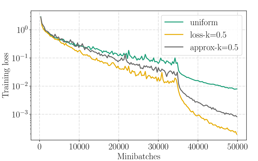
(a) Speed-up per epochs

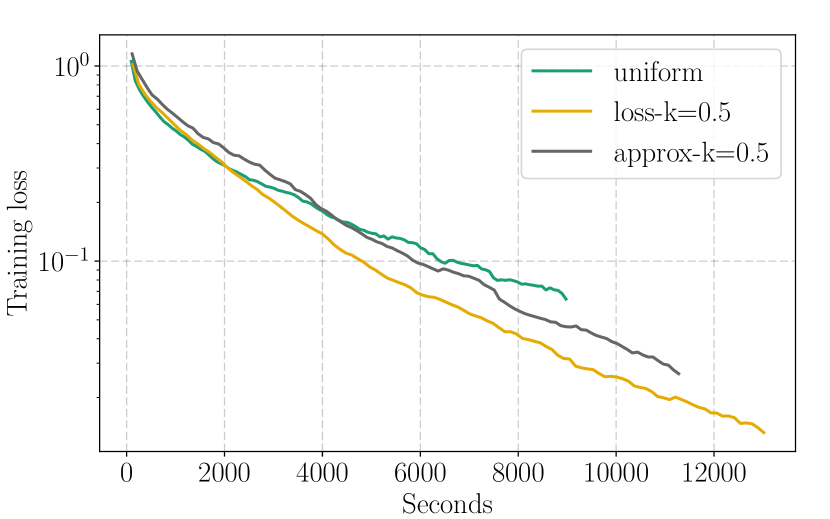
(b) Wall-clock time Speed-up

Figure 2: Training evolution results for CIFAR10 (average of $3$ runs). Figure 2(a) depicts the speed-up achieved with importance sampling in terms of epochs while Figure 2(b) shows the wall-clock time improvement achieved with importance sampling for the first $35,000$ iterations of training (before the learning rate reduction). Figure 2(b) shows an 11-point moving average.

In this section, we analyze experimentally the behaviour of the proposed importance sampling schemes. In the first subsection, we show the variance reduction followed by a comparison with the sampling using the gradient norm and an analysis of the effects of the hyperparameter $k$ (from equation 9), which controls the bias. In the following subsections, we present the attained improvements in terms of training time and test error reduction compared to uniform sampling. For our experiments, we use three well known benchmark datasets, MNIST (?), CIFAR10 (?) and Penn Treebank (?).

We compare the proposed sampling strategies, loss, which uses the actual model to calculate the importance and approx, which uses our approximation defined in the previous sections to uniform sampling which is our baseline and gnorm that uses the gradient norm as the importance.

In particular, the approx is implemented using an LSTM with a hidden state of size $32$. The input to the LSTM layer is at most the $10$ previously observed loss values of a sample (features of one dimension). Regarding the class label, it is initially projected in $\mathbb{R}^{32}$ and subsequently concatenated with the hidden state of the LSTM. The resulting $64$ dimensional feature is used to predict the loss with a simple linear layer.

In all the experiments, we deviate slightly from our theoretical analysis and algorithm by sampling mini-batches instead of single samples in line 6 of Algorithm 1, and using the Adam optimizer (?) instead of plain Stochastic Gradient Descent in lines 8 and 9 of Algorithm 1.

Experiments were conducted using Keras (?) with TensorFlow (?), and the code to reproduce the experiments will be provided under an open source license when the paper will be published. When wall clock time is reported, the experiment was run using an Nvidia K80 GPU and the reported time is calculated by subtracting the timestamps before starting one epoch and after finishing one; thus it includes the time needed to transfer data between CPU and GPU memory.

Behaviour of loss-based Importance Sampling

In this section, we present an in-depth analysis of our biased importance sampling, by performing experiments on the well know hand-written digit classification dataset, MNIST. Given the simplicity of the dataset, we choose a down-sized variant of the VGG architecture (?), with two convolutional layers with $32$ filters of size $3\times 3$, a max-pooling layer and a dropout layer with a dropout rate of $0.25$, without batch normalization, followed by the same combination of layers with twice the number of filters. Finally, we add two fully connected layers with $512$ neurons and dropout with rate $0.5$, and a final classification layer. All the layers use the ReLU activation function.

Comparison with the gradient norm

The first experiment of this section compares the loss to the gradient norm as importance metrics. We train each network for $6,000$ iterations with a mini-batch size of $128$. For each set of parameters we run $10$ independent runs with different random seeds and report the average. For the pre-sampling of Algorithm 1 we use $2B$ where $B$ is the size of the mini-batch, so in this case the importance is computed for $256$ randomly selected samples per parameter update.

In Figure 1(a), we observe that our importance sampling scheme accelerates the training in terms of epochs by $6\times$. It is also evident that the variance is reduced compared to uniform sampling. In this experiment, we observed that sampling with the gradient norm is more than $100$ times slower, with respect to wall-clock time, than sampling using the loss. Moreover, compared to the optimal sampling using the gradient norm, we show that gradient norm is very sensitive to randomness introduced by the Dropout layers and thus performs a bit worse than our proposed method. The above could be one of the reasons why no other work has ever used the gradient norm to train Deep Neural Network models with Dropout or Batch Normalization.

Analysis of the sampling bias

Using the loss as the importance metric for sampling our mini-batches allows us to efficiently minimize a surrogate to a soft max-loss, namely the original loss raised to the power $2-k$ (see equation 13). We theorize (based on (?)) that minimizing such a loss will be beneficial to the generalization ability of the trained model. Although this will be empirically tested in the last section of the experiments, in this section, we aim to empirically validate our theory that using a small $k$ focuses on the max-loss of the dataset.

For this experiment, we train, again, each network for $6,000$ iterations with $k\in\{0,0.5,0.75,1\}$. Every $300$ iterations, we compute the loss for each image in the training set. Figure 1(b) depicts the moving average of the maximum loss for all the parameter combinations. We observe that smaller values for $k$, indeed, minimize the maximum loss while $k=1$, which corresponds to unbiased importance sampling, ignores the maximum loss in the same way that uniform sampling does. In addition, using $k<0$ has been observed to result in noisy training, which can be explained by the fact that we increase the gradients of the samples with large gradient norm, thus resulting in very big steps per iteration. Due to the above, we use $k=0.5$ for all subsequent experiments, which has been found to be a good compromise between variance reduction and max-loss minimization.

Convergence speed-up

 

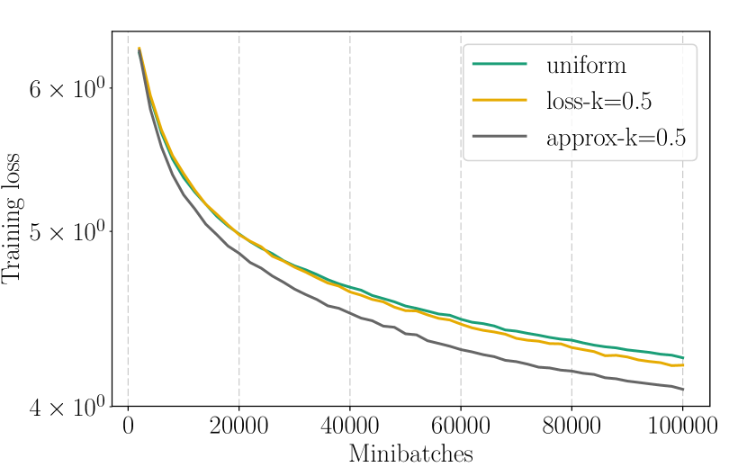
(a) Speed-up per epochs

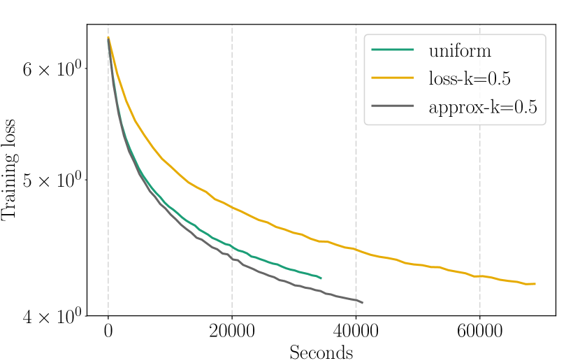
(b) Wall-clock time Speed-up

Figure 3: Training evolution results for Penn Treebank for $100,000$ iterations (average of $3$ runs). Figure 3(a) depicts the speed-up achieved with importance sampling in terms of epochs while Figure 3(b) shows the wall-clock time improvement.

Our second series of experiments aim to show the convergence speed-up achieved by sampling according to the loss (loss) and by our fast approximation trained alongside the full model (approx). To that end we perform experiments on CIFAR10 (?), an image classification dataset commonly used to evaluate new Deep Learning methods, and Penn Treebank (?), a widely used word prediction dataset.

Image classification

For the CIFAR10 dataset, we developed a VGG-inspired network, with batch normalization, which consists of three convolution-pooling blocks with $64$, $128$ and $256$ filters, two fully connected layers of sizes $1024$ and $512$, and a classification layer. Dropout is used in a similar manner as for the MNIST network with rates $0.25$ after each pooling layer and $0.5$ between the fully connected layers. The activation function in all layers is ReLU.

To compare the performance of the methods with respect to training epochs, each network is trained for $50,000$ iterations using a batch size of $128$ samples. After $35,000$ iterations we decrease the learning rate by a factor of $10$. We perform minor data augmentation by creating $500,000$ images generated by random flipping, horizontal and vertical shifting of the original images. For the importance sampling strategies, we use smoothing as described in the previous sections. In particular, the importance of each sample is incremented by $\frac{1}{2}\bar{L}$, where $\bar{L}$ is the mean of the training loss computed by the exponential moving average of the mini-batch losses. Furthermore, we run each method with $3$ different random seeds and report the mean. Similar to the previous experiment, we calculate the importance on a uniformly sampled set twice the batch size and resample with importance (see line 6 Algorithm 1). The results, which are depicted in Figure 2(a), show that importance sampling accelerates the training significantly in terms of epochs, resulting in an order of magnitude better training loss after $50,000$ iterations.

In order for our proposed method to be useful as is, we need to achieve speed-up with respect to wall clock time as well as epochs. In Figure 2(b), we plot the training loss with respect to the seconds passed for the initial $35,000$ iterations of training for CIFAR10. The experiment shows that our approx model is $\sim 10\%$ faster than loss and $\sim 20\%$ slower than uniform per epoch. However, we observe that approx reaches the final loss attained with uniform sampling in $\sim 15\%$ less time while loss in $\sim 30\%$ less time shaving off approximately $45$ minutes out of the $2.5$ hours of training.

One of the reasons that our approximation does not perform as well can be explained by observing the first epochs in Figure 2(a) or the first seconds in Figure 2(b). Our approximation needs to collect information on the evolution of the losses in the set $\mathcal{H}_{t}$ (see equation 14); thus it does not perform well in the initial epochs. Moreover, the GPU handles very well the small $32\times 32$ images thus the full loss incurs less than $50\%$ slowdown per epoch compared to uniform sampling.

Word prediction

Table 1: Experimental results across all datasets and methods. The results are averaged over multiple runs ($10$ for MNIST and $3$ for CIFAR10 and Penn Treebank) and we report the mean and the standard deviation. For the Penn Treebank we report the perplexity in the validation set and for the rest the classification error. The learning rate is chosen to maximize the performance of the uniform sampling strategy for all cases. Runs labeled as loss use the trained model to predict the loss while approx use a smaller model to approximate the loss as defined in the previous sections. An epoch is defined as $300$ mini-batches for MNIST/CIFAR10, and $2000$ for Penn Treebank respectively.

Epoch Method Uniform Loss k=1 Loss k=0.5 Approx k=1 Approx k=0.5 MNIST 5 0.79% $\pm$ 0.11 0.73% $\pm$ 0.11 0.56% $\pm$ 0.04 0.83% $\pm$ 0.06 0.65% $\pm$ 0.05 10 0.64% $\pm$ 0.10 0.56% $\pm$ 0.07 0.52% $\pm$ 0.05 0.60% $\pm$ 0.06 0.61% $\pm$ 0.04 20 0.56% $\pm$ 0.07 0.53% $\pm$ 0.08 0.47% $\pm$ 0.04 0.53% $\pm$ 0.06 0.54% $\pm$ 0.06 CIFAR10 50 12.33% $\pm$ 0.39 10.68% $\pm$ 0.65 9.58% $\pm$ 0.16 11.54% $\pm$ 0.55 10.78% $\pm$ 0.09 100 10.19% $\pm$ 0.24 9.74% $\pm$ 0.44 9.20% $\pm$ 0.55 9.71% $\pm$ 0.14 9.90% $\pm$ 0.47 150 7.97% $\pm$ 0.10 7.77% $\pm$ 0.14 7.44% $\pm$ 0.14 7.61% $\pm$ 0.07 7.64% $\pm$ 0.27 PTB 10 184.5 $\pm$ 1.56 178.3 $\pm$ 2.47 187.2 $\pm$ 1.61 179.4 $\pm$ 6.20 180.0 $\pm$ 4.78 30 138.6 $\pm$ 0.60 137.8 $\pm$ 1.53 139.0 $\pm$ 0.72 136.2 $\pm$ 2.98 134.3 $\pm$ 2.19 50 130.3 $\pm$ 0.63 129.9 $\pm$ 1.27 130.5 $\pm$ 0.21 128.2 $\pm$ 2.02 127.4 $\pm$ 1.45   

To assess the generality of our method, we conducted experiments on a language modeling task. We used the Penn Treebank language dataset, as preprocessed by ? ̵̃(?), and a recurrent neural network as the language model. Initially, we split the dataset into sentences and add an “End of sentence” token (resulting in a vocabulary of 10,001 words). For each word we use the previous 20 words, if available, as context for the neural network. Our language model is similar to the small LSTM used by ? ̵̃(?) with 256 units, a word embedding in $\mathbb{R}^{64}$ and dropout with rate 0.5.

In terms of training the language models, we use a batch size of 128 words and train each network for $100,000$ iterations. For the importance sampling strategies, we use constant smoothing instead of adaptive as in the CIFAR10 experiment. To choose the smoothing constant, we experiment with the values $\{0.5,1,2.5\}$ and choose 0.5 because it performs better in terms of variance minimization during training. Finally, we run each method with 3 different random seeds and report the mean. Similar to the two previous experiments, we pre-sample uniformly 256 words, namely twice the mini-batch size.

The results of the language modeling experiment are presented in Figures 3(a) and 3(b). We observe (from Figure 3(a)), that using importance sampling indeed improves the convergence speed in terms of epochs. However, using the full loss performs marginally better than uniform random sampling. The gradient variance is reduced more using the actual model in this case as well, which leads us to the following two explanations:

1. A small amount of noise is beneficial to the training procedure (we could add noise to the loss method by increasing the smoothing parameter)

2. The slower changes in sample importance between iterations (side effect of using the history for our approximation) are beneficial to importance sampling

Moreover, it is important to note in Figure 3(b) that even if using the loss performed better with respect to epochs than approx, it requires twice as much time to train a given number of epochs compared to uniform. On the other hand, approx is merely $\sim 10\%$ slower per epoch, resulting $\mathbf{20\%}$ less time to achieve the final training loss, shaving almost $2$ hours from the $9.5$ hours required for uniform sampling to perform $100,000$ iterations.

We have also attempted to compare our method with the method presented by ? ̵̃(?). Although we managed to find a set of hyperparameters that achieve comparable speed-ups for CIFAR10, their method completely fails to converge for Penn Treebank, for the parameters we tested. This behaviour, reflects the experiments of the original paper and can possibly be explained by the ad-hoc aggressive weighting of samples that they employ.

Generalization improvement

In this experimental section we analyze the performance of the previously trained models on unseen data. Our goal is to show that importance sampling does not cause overfitting or affect the performance on the test set in any negative way.

Towards this end, we report the classification error on the test set for experiments conducted using the MNIST and CIFAR10 datasets while for the language modeling task we report the perplexity on the validation set. The results, for all the experiments, are summarized in Table 1, where the values are depicted for the early stages, medium stages and final stages of training.

We observe that the test error is the same or better than using uniform sampling in all cases. More importantly, Table 1 shows that our added bias is indeed helpful in reducing the generalization error, especially in the first stages of training. For MNIST we observe a $0.2\%$ reduction in error at the 5-th epoch when using $k=0.5$ and for CIFAR10 approximately $1\%$ at the 30-th epoch. For Penn Treebank the case is not as clear although we observe a reduction of $2$ at the 30-th epoch when compared to the approx method with $k=1$.

Finally, we have empirically observed that using $k=0.5$ results in a robust procedure that requires less smoothing and is affected less by noisy importance estimation.

Conclusion

In this paper, we show theoretically and empirically that the loss can be used as an importance metric to accelerate the training of any Deep Neural Network architecture including recurrent ones. In particular, we propose a biased importance sampling scheme (with and without a lightweight approximation), that results in significant speed-up both in terms of wall-clock time and epochs. Using this sampling scheme, we train Deep Neural Networks for image classification and word prediction tasks $20\%$ to $30\%$ faster than using uniform sampling with Adam.

Two important points remain to be investigated thoroughly. The first is the construction of a more principled method to approximate the loss of the full model. Modern neural networks contain hundreds of layers; thus it is hard to imagine that there exists no approximation to their output that can fully take advantage of the cost/accuracy trade-off.

The second point is the exploitation of the reduced variance of the gradient estimator by some other part of the stochastic optimization procedure. Importance sampling, for instance, could be used to perform stochastic line search or improve the robustness of stochastic Quasi-Newton methods.

Appendix

Appendix A Justification for sampling with the loss

The goal of this analysis is to justify the use of the loss as the importance metric instead of the gradient norm and provide additional evidence (besides the experiments in the paper) that it is an improvement over uniform sampling.

Initially, we show that sampling with the loss is better at minimizing an upper bound to the variance of the gradients than uniform sampling. Subsequently, we provide additional empirical evidence that the loss is a surrogate for the gradient norm by computing the exact gradient norm for a limited number of samples and comparing it to the loss.

Theoretical justification

Initially, we show in lemma 2 that the most common loss functions for classification and regression define the same ordering as their gradient norm. Subsequently, we use this derivation together with an upper bound to the variance of the gradients and show that sampling according to the loss reduces this upper bound compared to uniform sampling.

Firstly, we prove two lemmas that will be later used in the analysis.

Lemma 1.

Let $f(x):\mathbb{R}\to\mathbb{R}$ be a strictly convex monotonically decreasing function then

$$f(x_{1})>f(x_{2})\iff\left|\frac{\partial f}{\partial x_{1}}\right|>\left|\frac{\partial f}{\partial x_{2}}\right|\ \forall\ x_{1},x_{2}\in\mathbb{R}.$$ (15)

Proof.

By the definition of $f(x)$ we have

$$\frac{\partial^{2}f}{\partial x^{2}}>0\ \forall\ x$$ (16)

$$\frac{\partial f}{\partial x}\leq 0\ \forall\ x,$$ (17)

which means that $\frac{\partial f}{\partial x}$ is monotonically increasing and non-positive. In that case we have

$$x_{1}<x_{2} \iff f(x_{1})>f(x_{2})$$ (18)

$$x_{1}<x_{2} \iff\frac{\partial f}{\partial x_{1}}<\frac{\partial f}{\partial x_{2}}\iff\left|\frac{\partial f}{\partial x_{1}}\right|>\left|\frac{\partial f}{\partial x_{2}}\right|$$ (19)

therefore proving the lemma. ∎

Lemma 2.

Let $L(\psi):D\to\mathbb{R}$ be either the negative log likelihood or the squared error loss function defined respectively as

$$L_{1}(\psi) =-y^{T}log(\psi) y\in\{0,1\}^{d}\ \text{s.t.}y^{T}y=1$$ (20)

$$D=[0,1]^{d}\ \text{s.t.}\left\lVert\psi\right\rVert_{1}=1$$

$$L_{2}(\psi) =\left\lVert y-\psi\right\rVert_{2}^{2} y\in\mathbb{R}^{d}\quad D=\mathbb{R}^{d}$$

where $y$ is the target vector. Then

$$L(\psi_{1})>L(\psi_{2})\iff\left\lVert\nabla_{\psi}L(\psi_{1})\right\rVert>\left\lVert\nabla_{\psi}L(\psi_{2})\right\rVert$$ (21)

Proof.

In the case of the squared error loss we have

$$\left\lVert\nabla_{\psi}L(\psi)\right\rVert_{2}^{2}=\left\lVert-2(y-\psi)\right\rVert_{2}^{2}=4L(\psi),$$ (22)

thus proving the lemma.

For the log likelihood loss we can use the fact that only one dimension of $y$ can be non-zero and prove it using lemma 1 because $f(x)=-log(x)$ is a strictly convex monotonically decreasing function. ∎

Main analysis

We can now prove theorem 2 which is also written below for completeness.

Theorem 2.

Let $G_{i}=\left\lVert\nabla_{\theta_{t}}L(\Psi(x_{i};\theta_{t}),y_{i})\right\rVert$ and $M=\max G_{i}$. There exist $K>0$ and $C<M$ such that

$$\frac{1}{K}L(\Psi(x_{i};\theta_{t}),y_{i})+C\geq G_{i}\quad\forall i$$ (23)

Proof.

The goal of importance sampling is to minimize

$$\text{Tr}\left(\operatorname{\mathbb{V}}\left[\nabla_{\theta}L(\Psi(x_{i};\theta),y_{i})\right]\right)=\operatorname{\mathbb{E}}\left[\left\lVert\nabla_{\theta}L(\Psi(x_{i};\theta),y_{i})\right\rVert_{2}^{2}\right].$$ (24)

To perform importance sampling, we sample according to the distribution $P$ with probabilities $p_{i}$ and use per sample weights $\alpha_{i}=\frac{1}{Np_{i}}$ in order to have an unbiased estimator of the gradients. Consequently, the variance of the gradients is

$$\operatorname{\mathbb{E}}_{P}\left[\left\lVert\alpha_{i}\nabla_{\theta}L(\Psi(x_{i};\theta),y_{i})\right\rVert_{2}^{2}\right] =$$ (25)

$$\sum_{i=1}^{N}p_{i}\alpha_{i}^{2}\left\lVert\nabla_{\theta}L(\Psi(x_{i};\theta),y_{i})\right\rVert_{2}^{2} =$$ (26)

$$\sum_{i=1}^{N}\frac{1}{Np_{i}}\frac{1}{N}\left\lVert\nabla_{\theta}L(\Psi(x_{i};\theta),y_{i})\right\rVert_{2}^{2} =$$ (27)

$$\sum_{i=1}^{N}\alpha_{i}\frac{1}{N}\left\lVert\nabla_{\theta}L(\Psi(x_{i};\theta),y_{i})\right\rVert_{2}^{2}.$$ (28)

Assuming that the neural network is Lipschitz continuous (assumption that holds when the weights are not infinite) with constant $K$, we derive the following upper bound to the variance

$$\operatorname{\mathbb{E}}_{P}\left[\left\lVert\alpha_{i}\nabla_{\theta}L(\Psi(x_{i};\theta),y_{i})\right\rVert_{2}^{2}\right]\leq$$ (29)

$$\sum_{i=1}^{N}\alpha_{i}\frac{1}{N}\left\lVert\nabla_{\theta}\Psi(x_{i};\theta)\right\rVert_{2}^{2}\left\lVert\nabla_{\Psi(x_{i};\theta)}L(\Psi(x_{i};\theta),y_{i})\right\rVert_{2}^{2}\leq$$ (30)

$$K^{2}\sum_{i=1}^{N}\alpha_{i}\frac{1}{N}\left\lVert\nabla_{\Psi(x_{i};\theta)}L(\Psi(x_{i};\theta),y_{i})\right\rVert_{2}^{2}.$$ (31)

Since we have a finite set of samples, there exists a constant $C$ such that

$$L(\Psi(x_{i};\theta),y_{i})+C \geq\left\lVert\nabla_{\Psi(x_{i};\theta)}L(\Psi(x_{i};\theta),y_{i})\right\rVert$$ (32)

$$\forall\ i\in\{1,2,\dots,N\}.$$

However, using lemma 2 we know that this upper bound is better than uniform because $L(\Psi(x_{i};\theta),y_{i})$ and $\left\lVert\nabla_{\Psi(x_{i};\theta)}L(\Psi(x_{i};\theta),y_{i})\right\rVert$ grow and shrink in tandem. In particular the following equation holds, where $M=\max\left\lVert\nabla_{\Psi(x_{i};\theta)}L(\Psi(x_{i};\theta),y_{i})\right\rVert$ and $C<M$

$$L(\Psi(x_{i};\theta),y_{i})+C-\left\lVert\nabla_{\Psi(x_{i};\theta)}L(\Psi(x_{i};\theta),y_{i})\right\rVert<$$ (33)

$$M-\left\lVert\nabla_{\Psi(x_{i};\theta)}L(\Psi(x_{i};\theta),y_{i})\right\rVert\quad\forall i.$$

Using equations 31, 32 and 33 and replacing the constants in 31 with $K$ we derive the original claim concluding the proof. ∎

Empirical justification

In this section, we provide empirical evidence regarding the use of the loss instead of the gradient norm as the importance metric. Specifically, we conduct experiments computing the exact gradient norm and the loss value for the first 20,000 samples during training. The gradient norm is normalized in each mini-batch to account for the changes in the norm of the weights.

Subsequently, we plot the loss sorted by the gradient norm. If there exists $C$ such that $L(\Psi(x_{i};\theta),y_{i})=C\left\lVert\nabla_{\theta}L(\Psi(x_{i};\theta),y_{i})\right\rVert$ we should see approximately a line. In case of order preservation we should see a monotonically increasing function.

   

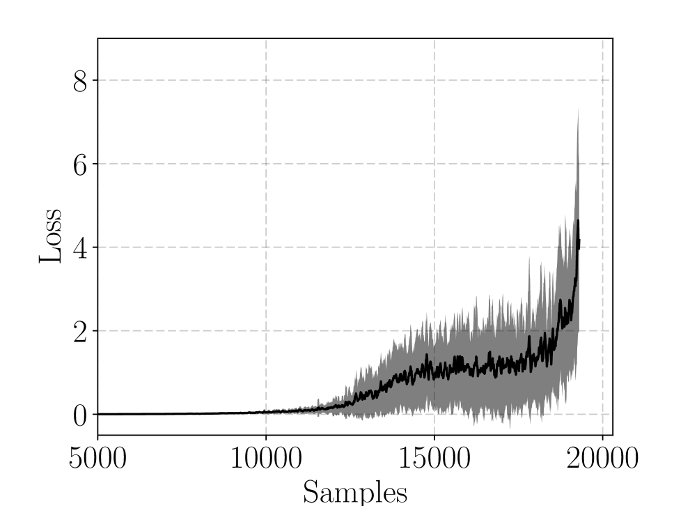
(a) MNIST

(b) CIFAR10

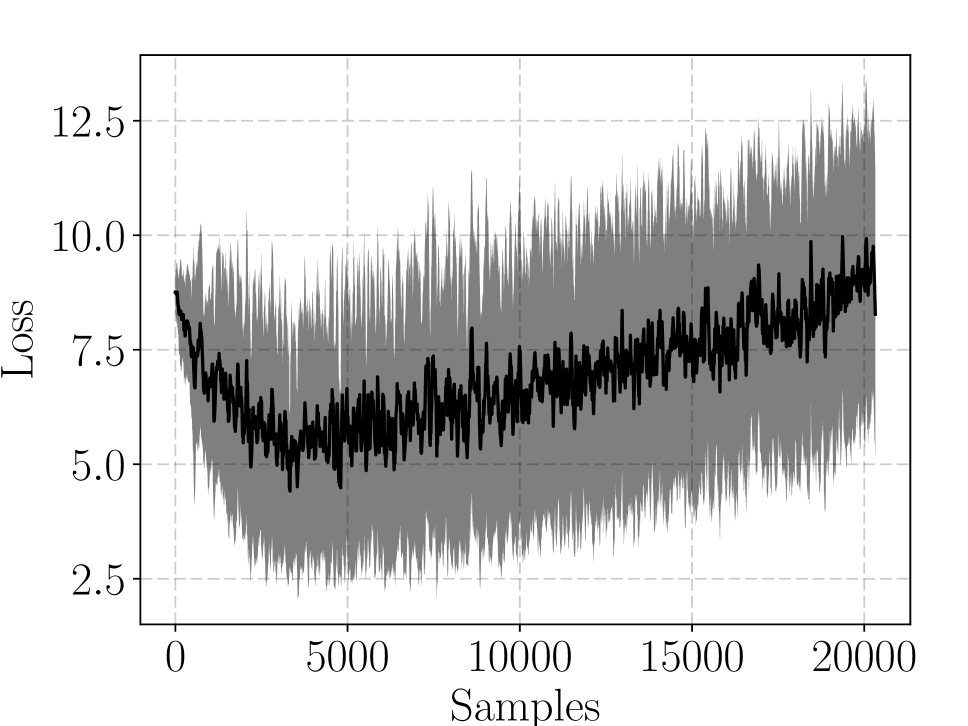
(c) Penn Treebank

Figure 4: Loss values sorted by gradient norm. The solid line is a moving average ($50$ samples window) and the shaded area denotes one standard deviation.

In figure 4, we observe a correlation between the gradient norm and the loss. In all cases, samples with high gradient norm also have high loss. In the Penn Treebank dataset, (Figure 4(c)), there exist some samples with high loss but very low gradient norm. This can be explained because LSTMs use the $\text{tanh}(\cdot)$ activation function which can have very low gradient but incorrect output. We note that this cannot hurt performance, it just means that we waste some CPU/GPU cycles on samples that are incorrectly classified but will not affect the parameters heavily.

Appendix B Loss tracking by our approximation

In this section, we present empirical evidence that the proposed approximate model predicts the loss with reasonable accuracy. In order to describe the experiment, we introduce the following notation. Let $\hat{L}_{i}$ be the loss value computed for the $i$-th sample and used as importance in the sampling procedure. In addition, let $L_{i}$ be the loss computed in the forward pass of the optimization procedure, with the same parameters and for the same sample. As mentioned in the paper, $L_{i}$ and $\hat{L}_{i}$ can differ even if we use the full network to compute $\hat{L}_{i}$, due to stochasticity introduced by Dropout layers and Batch Normalization.

To compute how well $\hat{L}_{i}$ “tracks” $L_{i}$ we solve the following least squares problem for every minibatch. The value of the coefficient $a$ shows how well $\hat{L}_{i}$ approximates $L_{i}$.

$$a^{*},b^{*}=\operatorname*{arg\,min}_{a,b}\sum_{i\in B}\left(a\hat{L}_{i}+b-L_{i}\right)^{2}$$ (34)

In Figure 5, we present the evolution of the coefficient $a$ for the experiments in CIFAR10 and Penn Treebank. Regarding CIFAR10, we observe that the loss is really hard to track, even using the full Neural Network. However, the approximation presents a positive correlation with $L_{i}$ which appears to be enough for reducing the variance of the gradients. Moreover, after $15,000$ mini-batches the approximation “tracks” the loss with the same accuracy as the full network. On the other hand, in the Penn Treebank experiment, there seems to be less noise and $L_{i}$ is predicted accurately by both methods. Once again, we observe, that as the training progresses our approximation seems to converge towards the same quality of predictions as using the full network.

   

(a) CIFAR10

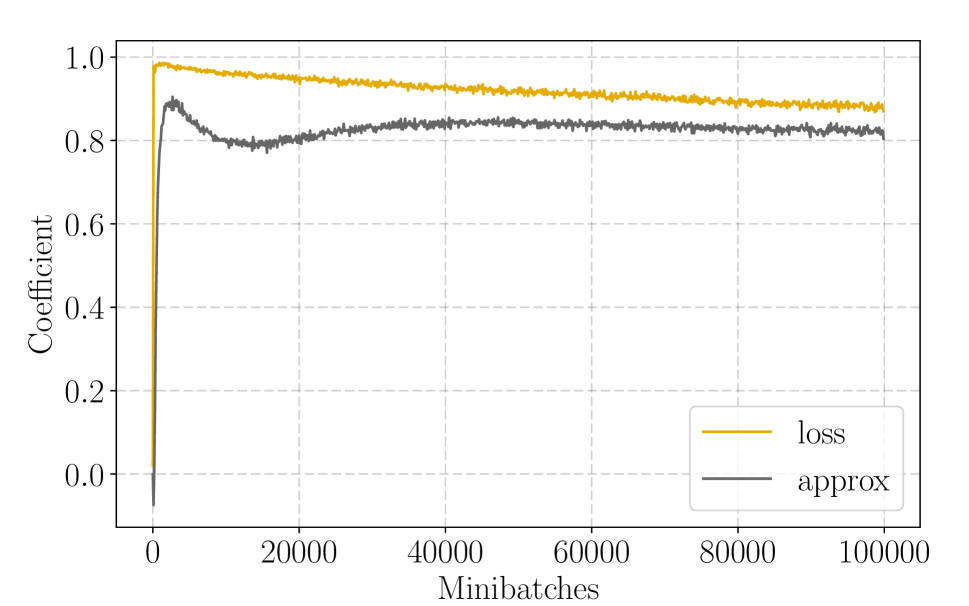
(b) Penn Treebank

Figure 5: The coefficient $a$ from equation 34 is plotted for loss and approx. A coefficient value of $1$ means that the loss is tracked perfectly while $0$ means almost uniform sampling. Due to randomness introduced by layers such as Dropout and Batch Normalization, even using the full network (loss) does not mean perfect prediction.

References

- [2016] Abadi, M.; Agarwal, A.; Barham, P.; Brevdo, E.; Chen, Z.; Citro, C.; Corrado, G. S.; Davis, A.; Dean, J.; Devin, M.; et al. 2016. Tensorflow: Large-scale machine learning on heterogeneous distributed systems. arXiv preprint arXiv:1603.04467.
- [2015] Alain, G.; Lamb, A.; Sankar, C.; Courville, A.; and Bengio, Y. 2015. Variance reduction in sgd by distributed importance sampling. arXiv preprint arXiv:1511.06481.
- [2009] Bengio, Y.; Louradour, J.; Collobert, R.; and Weston, J. 2009. Curriculum learning. In Proceedings of the 26th annual international conference on machine learning, 41–48. ACM.
- [2005] Bordes, A.; Ertekin, S.; Weston, J.; and Bottou, L. 2005. Fast kernel classifiers with online and active learning. Journal of Machine Learning Research 6(Sep):1579–1619.
- [2016] Canévet, O.; Jose, C.; and Fleuret, F. 2016. Importance sampling tree for large-scale empirical expectation. In Proceedings of the International Conference on Machine Learning (ICML), 1454–1462.
- [2015] Chollet, F., et al. 2015. keras. https://github.com/fchollet/keras.
- [2014] Kingma, D., and Ba, J. 2014. Adam: A method for stochastic optimization. arXiv preprint arXiv:1412.6980.
- [2009] Krizhevsky, A. 2009. Learning multiple layers of features from tiny images. Master’s thesis, Department of Computer Science, University of Toronto.
- [2010] Kumar, M. P.; Packer, B.; and Koller, D. 2010. Self-paced learning for latent variable models. In Advances in Neural Information Processing Systems, 1189–1197.
- [1998] LeCun, Y.; Cortes, C.; and Burges, C. J. 1998. The mnist database of handwritten digits.
- [2015] Loshchilov, I., and Hutter, F. 2015. Online batch selection for faster training of neural networks. arXiv preprint arXiv:1511.06343.
- [1993] Marcus, M. P.; Marcinkiewicz, M. A.; and Santorini, B. 1993. Building a large annotated corpus of english: The penn treebank. Computational linguistics 19(2):313–330.
- [2011] Mikolov, T.; Deoras, A.; Kombrink, S.; Burget, L.; and Černockỳ, J. 2011. Empirical evaluation and combination of advanced language modeling techniques. In Twelfth Annual Conference of the International Speech Communication Association.
- [2014] Needell, D.; Ward, R.; and Srebro, N. 2014. Stochastic gradient descent, weighted sampling, and the randomized kaczmarz algorithm. In Advances in Neural Information Processing Systems, 1017–1025.
- [2013] Richtárik, P., and Takáč, M. 2013. On optimal probabilities in stochastic coordinate descent methods. arXiv preprint arXiv:1310.3438.
- [2016] Shalev-Shwartz, S., and Wexler, Y. 2016. Minimizing the maximal loss: How and why. In Proceedings of the 32nd International Conference on Machine Learning.
- [2014] Simonyan, K., and Zisserman, A. 2014. Very deep convolutional networks for large-scale image recognition. CoRR abs/1409.1556.
- [2016] Wang, L.; Yang, Y.; Min, M. R.; and Chakradhar, S. 2016. Accelerating deep neural network training with inconsistent stochastic gradient descent. arXiv preprint arXiv:1603.05544.
- [2014] Zaremba, W.; Sutskever, I.; and Vinyals, O. 2014. Recurrent neural network regularization. arXiv preprint arXiv:1409.2329.
- [2015] Zhao, P., and Zhang, T. 2015. Stochastic optimization with importance sampling for regularized loss minimization. In Proceedings of the 32nd International Conference on Machine Learning (ICML-15), 1–9.