Evolution from few- to many-body physics in one-dimensional Fermi systems:
One- and two-body density matrices and particle-partition entanglement
Abstract
We study the evolution from few- to many-body physics of fermionic systems in one spatial dimension with attractive pairwise interactions. We determine the detailed form of the momentum distribution, the structure of the one-body density matrix, and the pairing properties encoded in the two-body density matrix. From the low- and high-momentum scaling behavior of the single-particle momentum distribution we estimate the speed of sound and Tan’s contact, respectively. Both quantities are found to be in agreement with previous calculations. Based on our calculations of the one-body density matrices, we also present results for the particle-partition entanglement entropy, for which we find a logarithmic dependence on the total particle number.
pacs:
03.65.Ud, 05.30.Fk, 03.67.MnI Introduction
In the last decade, the detailed experimental study of ultracold atoms has revealed a stunning array of phenomena in a wide range of situations. The ever-growing ability to control and measure the properties of atomic clouds has enabled the study of fermionic and bosonic systems in one, two, and three dimensions, lattices, and even mixed dimensions by carefully tuning external trapping potentials (see, e.g., Refs. Bloch et al. (2008); Haller et al. (2010); Liao et al. (2010)). As is well known, that versatility extends to changes in the interaction strength via Feshbach resonances Wu and Thomas (2012) as well as to control over the degree of polarization (pseudo-spin population imbalance) and mass asymmetry (by isotopic variations). Such an unprecedented plasticity makes the investigation of the challenging strongly coupled regimes both urgent and necessary.
On the computational side, the quantitative characterization of these quantum few- and many-body systems poses a formidable challenge. The complexity of quantum many-body physics presents itself in two ways. In non-stochastic methods, such as exact diagonalization, the memory requirements scale factorially with the size of the system (number of particles or spatial volume, depending on the algorithm), simply because that is how the dimension of the Hilbert space grows. In stochastic methods, namely quantum Monte Carlo (QMC) and all its incarnations, full access to eigenstates is relaxed in exchange for answers to specific questions (i.e. specific correlation functions) and so the memory limitations are much milder.
As far as computations of properties of 1D systems are concerned, there are several non-stochastic ways to arrive at the ground-state properties, such as the Bethe ansatz Guan et al. (2013), (density-matrix) renormalization group approaches Voit (1995); *RevModPhys.77.259, exact diagonalization Sowiński et al. (2013); *0295-5075-109-2-26005; *PhysRevA.94.042118, methods based on effective interactions Lindgren et al. (2014) as well as coupled-cluster approaches frequently applied in quantum chemistry Grining et al. (2015).
One of the main objectives of the present work is to set benchmarks that show quantitatively and in detail what is presently feasible with our lattice QMC approach. To this end, we expand on previous works Rammelmüller et al. (2015); Loheac et al. (2015) and consider a model for two-component Fermi gases in one dimension with an attractive contact interaction between the two species (see Sec. II for a brief discussion), focusing on systems with an equal population of spin-up and spin-down fermions. The algorithm we use relies on an auxiliary field transformation to decouple the spin species in the density channel. This allows for a relatively simple calculation of the one-body density matrix as well as the on-site two-body density matrix (i.e. the pair-correlation function). However, the latter requires taking the square of the one-body density matrix for each auxiliary field configuration, which increases the statistical noise significantly. Therefore, better statistics are needed to obtain a more accurate estimate for this quantity, which can be most easily tested and achieved in the one-dimensional (1D) limit.
In Sec. III, we present fully non-perturbative calculations of the one- and two-body density matrices along with the associated momentum distributions for our 1D system of fermions. We compute these quantities in the ground state for different particle content and across a number of coupling strengths ranging from the noninteracting case to the strongly-coupled regime. The fact that this specific problem is in principle exactly solvable by way of the Bethe ansatz Bethe (1931) is of great importance to us as it allows to benchmark our lattice QMC approach, e.g. with respect to the computation of the ground-state energy and the speed of sound. Since the exact analytic approaches successfully employed over decades in the 1D case do not possess a straightforward generalization to higher-dimensional systems, our present study aims to set the methodological stage for future quantitative studies of one- and two-body density matrices of Fermi gases in higher dimensions. In particular, for future studies of systems with a finite spin- and mass-imbalance, the computation of general correlation functions is of interest as the formation of an inhomogeneous ground state is expected to leave its imprint on these quantities, see, e.g., Refs. Casula et al. (2008); Lee and Guan (2011); Roscher and Braun (2016). Although our present 1D study does not fully generalize to higher dimensions, e.g. with respect to the scaling of the observables with the lattice size, we still consider it useful from a methodological point of view as it is possible to take vastly more data than in higher dimensions. This allows us to test how our algorithms perform against the background of the existing exact results in the 1D limit.
From a phenomenological point of view, 1D Fermi gases allow to study the transition from few- to many-body physics in detail, both experimentally Wenz et al. (2013); *2013PhRvL.111q5302Z and theoretically (see Ref. Zinner (2016) for a review). The exploration of this transition has been enriched by the concepts of quantum information, such as entanglement, entanglement entropy, mutual information, as well as corresponding methods to determine them. We rush to add that a direct comparison of our present results to experimental data would be qualitative at best. Indeed, we shall consider fermions in a box with periodic boundary conditions since they have been found to minimize finite-volume effects in relativistic model studies in the sense that the infinite-volume limit is approached faster than in case of antiperiodic boundary conditions (see, e.g., Ref. Braun et al. (2005)). Of course, the latter are only one representative of boundary conditions which do not allow for a zero-momentum mode. A rigorous proof of this observation for general boundary conditions and observables is difficult, if possible at all. In any case, for a quantitative comparison with experimental data in the future (in particular with respect to the few-body limit), the numerical implementation of trap potentials Berger et al. (2015, 2016) as used in experiments will be required. For example, harmonic traps are often considered in 1D experiments Wenz et al. (2013); *2013PhRvL.111q5302Z. Interestingly, we note that the realization of flat-bottom traps in experiments has now also become possible (see e.g. Hueck et al. (2017)). Compared to systems with periodic boundary conditions, however, the computational cost at fixed system size for studies involving such trapping geometries has been found to increase Berger et al. (2016); McKenney et al. (2016) in case of our present MC approach.
As a direct and nontrivial application of our results for the density matrix, we are able to push further and explore specific quantum-information aspects of this system by computing the one-particle partition-entanglement entropy. The so-called Rényi entanglement entropy has been a center of attention for the last few years as a possible order parameter for topological phase transitions Amico et al. (2008); *RevModPhys.81.865. Indeed, it was found that the so-called area-law violation (specifically, a logarithmic modification to the expected area law scaling with sub-system size) could signal such a phase change Eisert et al. (2010). Our motivation for considering the particle partition form of the Rényi entanglement entropy is based on the recent interest in this quantity and its scaling with the system size, which has been empirically found to follow a logarithmic law as in the case of spatial entanglement Haque et al. (2009); *PhysRevB.76.125310; *PhysRevLett.98.060401; Zozulya et al. (2008); Barghathi et al. (2017). While conventional studies of entanglement analyze the degree of spatial entanglement of a sub-system, circumscribed by a specific region of space, with the rest of the system, the kind of entanglement we study here is different. Particle-partition entanglement quantifies the degree of quantum correlation between a sub-set of particles (identified by labels of the density matrix) and the rest of the particles in the system. As in the case of spatial entanglement, the quantum correlation being measured includes statistical effects, which are non-trivial even for non-interacting systems. However, particle-partition entanglement features non-universal coefficients in the leading logarithms that vary with the particle statistics as well as with the interaction strength, which makes it a useful diagnostic tool for quantum correlations in strongly coupled matter Zozulya et al. (2008); Barghathi et al. (2017).
II Model and Scales
We focus on the attractive regime of the unpolarized Gaudin-Yang model Yang (1967); *GAUDIN196755 in a finite box with periodic boundary conditions which, in first quantization, is given by the Hamiltonian
| (1) |
The coupling is related to the -wave scattering length , , see, e.g., Ref. Barlette et al. (2000). We use conventions such that corresponds to an attractive interaction and work in units where with being the mass of the fermions, equal for both spins. As previously mentioned, our attention is restricted to the case with two fermion species interacting via a contact interaction, an example for a Luttinger liquid Luttinger (1963). For our ground-state calculations, we employ the techniques previously used in Refs. Rammelmüller et al. (2015); Drut (2012); Rammelmüller et al. (2016). Specifically, we formulate the given quantum many-body problem on a discretized Euclidean spacetime of dimensionless extent . Using a symmetric Trotter-Suzuki decomposition followed by an auxiliary field transformation, we arrive at path-integral expressions for our desired observables, which we evaluate via the Hybrid Monte Carlo (HMC) algorithm.
The calculations presented in this work have been carried out by projecting the ground state out of a guess wave function of fixed particle number . This even integer along with the ring circumference with lattice spacing and the attractive coupling strength comprise the physical input parameters where only the latter two are dimensionful. As is typical in 1D ground-state studies, from these two quantities we define a single intensive dimensionless parameter , where is the particle-number density. The extent of the imaginary time direction is , defining as the temporal lattice spacing. Therefore an extrapolation to the large limit is required, where and . Note that, in all cases, we have fixed the (spatial) lattice spacing to unity, which sets the length and momentum scales.
III Results
In this section, we discuss our results for all previously mentioned observables as a function of the dimensionless coupling . In general, we took lattice sites, consistent with previous studies for the 1D ground state Rammelmüller et al. (2015). Results were obtained by averaging decorrelated samples. Typical autocorrelation times for the total energy are of the order of and the sampling frequency of order , to ensure decorrelation also for other quantities under study. Unless otherwise noted, error estimates were obtained from statistical uncertainties by considering the standard deviation of the mean. For a discussion of lattice size and discretization effects, we refer the reader to the Appendix.
III.1 Ground-state energy
As a first cross-check, we re-computed the ground-state energy as a function of the coupling strength and particle number.
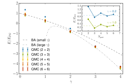
In Fig. 1, we compare our results for with the weak-coupling expansion,
| (2) |
and the strong-coupling expansion,
| (3) |
in the thermodynamic limit as obtained from the Bethe-ansatz Wadati and Iida (2007); Tracy and Widom (2016), where is the ground-state energy of the non-interacting two-component Fermi gas. We observe that our results are in excellent agreement with the weak-coupling expansion for and with the strong-coupling expansion for . Moreover, the thermodynamic limit appears to be approached rather rapidly, see also the inset of Fig. 1.
The exact (binding) energy of one spin-up and one spin-down fermion interacting via a contact interaction in the infinite-volume limit is given by Griffiths (2004), corresponding to . Thus, we observe that the ground-state energy per pair is simply given by the energy of the -body problem, , at leading order in the strong-coupling expansion. Loosely speaking, the dynamics in the strong-coupling limit may therefore be viewed as dominated by the formation of tightly bound pairs built up from one spin-up and one spin-down fermion. In the strict infinite-coupling limit , the many-body system can be viewed as a gas of composite bosons, the so-called Tonks-Girardeau gas Girardeau (1960).
In the weak-coupling limit, a finite gap has been found to emerge between the singlet ground state and the first triplet excited state together with gapless density fluctuations Lieb and Liniger (1963); *PhysRev.130.1616; Krivnov and Ovchinnikov (1965); Fuchs et al. (2004); Wadati and Iida (2007). Consequently, the dynamics of the many-body system in this limit is associated with a Bardeen-Cooper-Schrieffer (BCS) superfluid. For a detailed discussion of the many-body phase diagram, we refer the reader to Ref. Fuchs et al. (2004). Here, we only highlight that a smooth crossover from the formation of tight bosonic molecules in the limit to Cooper pairing in the limit is found to occur at in this system. At this point, the size of the bosonic pairs is of the order of the distance between the fermions Fuchs et al. (2004); Wadati and Iida (2007). Indeed, for the two-body problem in the infinite-volume limit, the “diameter" of the bosonic pair111We define the diameter as , where is the ground-state wave function. Note that is only a function of in the infinite-volume limit. is given by , see, e.g., Ref. Griffiths (2004). Thus, we have which may be viewed as a measure for the crossover point in terms of the coupling at which the properties of the system change significantly.
In the following subsections we do not aim at a detailed quantitative discussion of the phase diagram but focus on our results for the momentum distribution, the one- and two-body density matrices, and the particle partition entanglement entropy from few to many fermions.
.
III.2 One-body density matrix and momentum distribution
The one-body density matrix in principle allows us to compute all single-particle expectation values and is defined as ground-state expectation value of a creation and annihilation operator:
| (4) |
where refers to the spin index and the operators denote annihilation (creation) operators. In terms of a general -body wave function , the one-body density matrix associated with, e.g., the spin-up fermions is given by
| (5) |
and correspondingly for the spin-down fermions. The (single-particle) momentum distribution , i.e. the Fourier transform of the one-body density matrix, is implicitly defined as
| (6) |
where
| (7) |
and for the periodic box of extent considered in this work.
The one-body density matrix determines the overlap of a state, in which a fermion with spin has been removed from the ground state at point , with a state, in which a fermion with the same spin has been removed at point . Correspondingly, the associated single-particle momentum distribution determines the overlap of a state, in which a fermion with spin and momentum has been removed from the ground state, with a state, in which a fermion with the same spin but momentum has been removed. From the definition of the single-particle momentum distribution, it follows immediately that it is only finite for and in the non-interacting limit.
In a periodic box, the one-body density matrix of the non-interacting system can be computed analytically. We find
| (8) |
where for odd and for even .
For odd , we observe that the one-body density matrix of the non-interacting system is a translation-invariant quantity as it only depends on the distance between and . For even , however, the one-body density matrix of the non-interacting system is no longer translation-invariant in a periodic box but depends on and separately, see Eq. (8). Nevertheless, in the large- limit, the term breaking translation invariance is only subdominant, implying that the one-body density matrix becomes a translation-invariant quantity in the thermodynamic limit, as it should be. In fact, we have
| (9) |
for fixed with and .
We emphasize that the breaking of translation invariance in systems with even is a direct consequence of the fact that the ground-state wave function of the non-interacting system is not an eigenstate of the center-of-mass momentum operator ; it is, however, an eigenstate of . For odd , on the other hand, the ground-state wave function is an eigenstate of with zero eigenvalue.222As the Hamiltonian and parity operators commute with each other, the ground-state wave function (including the center-of-mass motion) can be chosen to be an eigenstate of the parity operator. Note that the part of the ground-state wave function describing the relative motion of the fermions has even parity whereas the parity of the center-of-mass wave function can be chosen at will. In our numerical implementation, conventions effectively correspond to choosing the center-of-mass wave function to have odd parity for even . For odd , we choose the center-of-mass wave function to have odd parity if is odd, and otherwise even. Since the ground-state wave function of the fully interacting system is effectively generated by exciting the ground-state wave function of the non-interacting system according to the momentum-conserving interaction, we conclude that translation invariance of the ground-state wave function is preserved in our QMC studies for systems with odd but is violated for systems with even , see also Ref. Kemler et al. (2017) for a discussion of this issue for systems in (anti)periodic boxes. We return to this below when discussing our results for the one-body density matrix.
From the one-body density matrix in Eq. (8), the momentum distribution of the non-interacting system is readily obtained. We find
| (10) | |||||
where for and otherwise.
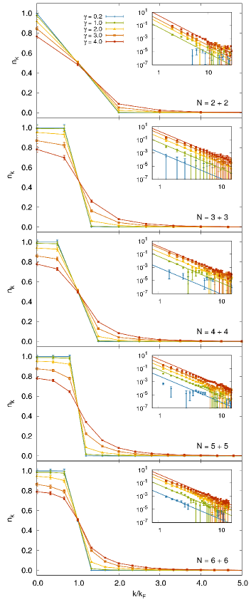
In Fig. 2, we show our results for the diagonal part of the momentum distribution as a function of for various particle numbers and coupling strengths . For small values of the coupling, , we observe that the momentum distribution is still well described by the non-interacting momentum distribution given in Eq. (10), independent of the total particle number . For stronger couplings, , the system is then dominated by the formation of tightly bound dimers where the crossover to this regime from the weakly coupled regime dominated by Cooper pairing occurs at , see our discussion in Sec. III.1. In the regime associated with , the momentum distributions clearly deviate from their non-interacting counterparts. More specifically, even states with very low momenta are now excited above the Fermi point . Loosely speaking, the momentum distributions effectively start to flatten out when the coupling is increased beyond and therefore these distributions lose their characteristic feature of a sharp drop present in the weak-coupling limit.
In order to further quantify the change in the momentum distributions when the coupling is increased, we analyze its scaling behavior close to the Fermi point . For spin-balanced systems, , and , the one-body density matrix in the thermodynamic limit is known to scale as follows Luther and Peschel (1974); Haldane (1981); Cazalilla (2004):
| (11) |
where . A comparison with the exact solution (9) for the free gas (i.e. ) immediately yields .
From Eq. (11), we obtain the scaling behavior of the single-particle momentum distribution (close) below the Fermi point in the thermodynamic limit, see also Ref. Giorgini et al. (2008):
| (12) |
The scaling exponent is directly related to the sound velocity of density fluctuations in our 1D Fermi gas. Indeed, we have with being the Fermi velocity Luther and Peschel (1974); Haldane (1981). With , we find for the free gas as expected.
For weak attractive interactions Krivnov and Ovchinnikov (1965), , the sound velocity is given by
| (13) |
whereas it reads
| (14) |
in the limit , i.e. in the strong-coupling limit Lieb and Liniger (1963). Assuming that the sound velocity is a monotonic function of the coupling , we conclude from these expansions that varies between at and in the limit . Recall our conventions for the sign of the coupling , see Eq. (1).
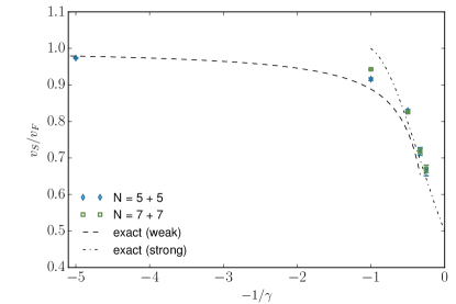
In this work, we exploit the scaling law (12) to estimate the sound velocity from a fit of our numerical data in the low-momentum regime to the ansatz based on the two parameters and . Of course, a high-precision determination of the low-momentum scaling behavior and the associated sound velocity requires to study larger particle numbers and even larger box sizes than considered in our present work in order to push the system closer to the thermodynamic limit.333In principle, the speed of sound can also be computed directly from the derivative of the chemical potential with respect to the density. However, the computation of the chemical potential defined as a derivative of the ground-state energy with respect to the particle number requires the computation of the ground-state energy of spin-imbalanced systems which is beyond the scope of the present work. Still, our present results for the sound velocity obtained from such a fit procedure already appear to be in reasonable agreement with the existing results for this quantity Fuchs et al. (2004), in particular with the weak- and strong coupling expansion given above, see Fig. 3. More specifically, we observe that the sound velocity remains close to the Fermi velocity for . For , the sound velocity then starts to decrease rapidly, suggesting that the systems enters the crossover regime between the “phase" dominated by Cooper pairing at small attractive couplings to a “phase" governed by the formation of a gas of tightly bound bosonic molecules, in accordance with earlier studies Fuchs et al. (2004).
| (this work) | (Ref. Rammelmüller et al. (2015)) | ||
|---|---|---|---|
| 2+2 | 0.2 | 0.003(1) | 0.00204(3) |
| 1.0 | 0.02(2) | 0.063(2) | |
| 2.0 | 0.36(2) | 0.35(1) | |
| 3.0 | 1.01(2) | 1.03(3) | |
| 4.0 | 2.3(3) | 2.36(2) | |
| 4+4 | 0.2 | 0.0013(2) | 0.00182(5) |
| 1.0 | 0.059(6) | 0.0582(6) | |
| 2.0 | 0.330(5) | 0.324(4) | |
| 3.0 | 0.99(3) | 0.99(1) | |
| 4.0 | 2.17(9) | 2.24(2) | |
| 6+6 | 0.2 | 0.0012(4) | 0.00178(3) |
| 1.0 | 0.055(2) | 0.0563(6) | |
| 2.0 | 0.33(1) | 0.311(4) | |
| 3.0 | 0.94(2) | 0.94(1) | |
| 4.0 | 2.20(8) | 2.14(2) |
We note that, as in the case of the ground-state energy, a fast convergence of our results to the thermodynamic limit is observed. In general, however, the convergence is faster for odd as terms violating translation invariance are absent in this case, see Eq. (8) and our discussion below.
Let us now turn to the scaling behavior of the momentum distribution at high momenta, which determines Tan’s contact density .444A detailed discussion of Tan’s relations for 1D systems can be found in Ref. Barth and Zwerger (2011). For the latter, we extracted estimates from the asymptotic behavior of the momentum distribution Tan (2008a); *Tan20082971; *Tan20082987,
| (15) |
by performing a linear fit of our results for for momenta with on a double-logarithmic scale, see also insets of Fig. 2. In our fits, we have only taken results for momenta with into account. Above this scale, we observe that the fits only exhibit a weak dependence on the actual fit range. Note that, for very dilute systems (i.e. small particle numbers) the high momentum part is subject to noise which explains the seemingly odd behavior at large momenta.
A priori, it is not evident where the above large-momentum asymptotics sets in. It was found in previous studies in 3D at unitarity Drut et al. (2011) that the onset scale is close to . In a QMC study of the corresponding 2D system Rammelmüller et al. (2016), it was observed that the onset scale increases with the coupling strength. At least in 1D, a rough estimate for this onset scale may be obtained by comparing the “diameter" of the bosonic bound state associated with the two-fermion problem with the de Broglie wavelength of a given fermion . The typical momentum of a fermion within the bound state may be estimated to be of the order of . This momentum scale should be compared to the momentum of a given fermion. If , then the fermion is not sensitive to the details of the short-range physics of our system but only to the long-range aspects. The long-range physics in our model is indeed immediately affected by an increase of the coupling, as indicated by our study of the scaling exponent of the single-particle momentum distribution determining the decay of the one-body density matrix in the long-range limit. If , then the fermion is sensitive to the details of the short-range physics of our 1D system. The latter case is associated with the dynamics which, e.g., determines Tan’s contact density.
In accordance with this simple argument, we indeed find in our numerical studies that the decay law sets in at higher scales when the coupling is increased for a fixed particle number, see also the insets of Fig. 2. In Tab. 1, results for the contact density for various couplings and particle numbers are provided. We note agreement with results previously obtained in Ref. Rammelmüller et al. (2015) for even using a different definition of Tan’s contact along with the Feynman-Hellmann theorem.
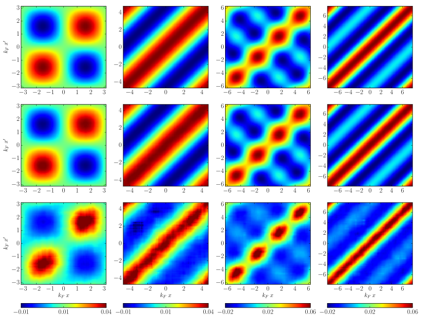
Finally, we discuss our results for the one-body density matrix being nothing but the Fourier transform of the momentum distribution , see Eq. 19. In Fig. 4, we present our results for as a function of the dimensionless coordinates and in a periodic box for fermions (from left to right) and (from top to bottom). The color coding is associated with the actual value of the one-body density matrix at the point . The results for finite represent numerical data from our QMC calculations, whereas the result for the non-interacting system () was obtained analytically, see Eq. (8).
The results shown in Fig. 4 exemplify our findings for other particle numbers. As suggested by the analytic solution (8) for the non-interacting limit, we observe that the number of oscillations at fixed coupling and box size increases with increasing particle number. The scale for these oscillations is set by the density. The main maxima of the one-body density matrix are found along the lines with , where . However, as already indicated above, we also clearly see that translation invariance is broken for even , whereas it is manifest for odd . This invariance is progressively restored as the particle number is increased. The mild violation of translation invariance for and odd in Fig. 4 is due to statistical uncertainties in our QMC calculations at strong couplings.
In Fig. 4, we also find that the width of the band associated with the lines of main maxima at is decreased with increasing coupling strength and the oscillations tend to flatten, leading to an increased localization of the one-body density matrix. This observation is consistent with the fact that the dynamics is governed by the formation of tightly bound bosonic molecules in the strong-coupling limit. Indeed, given our results for the single-particle momentum distribution, the increased localization of the one-body density matrix for increasing coupling strength does not come unexpected at all. It is, rather, a direct consequence of the fact that the single-particle momentum distribution is increasingly smeared out when is increased for fixed particle number. Quantitatively, this is measured by the increase of the critical exponent associated with the long-range scaling of the one-body density matrix, see Eq. (11), when is increased.
III.3 Pair-correlation function
In addition to the one-body density matrix, we have calculated the pair-correlation function, also known as the on-site two-body density matrix. In one-dimensional systems, this function has attracted a lot of interest for instance in the search for inhomogeneous ground states Casula et al. (2008). It is defined as
| (16) |
This expression can be rewritten in terms of the ground-state -body wave function :
| (17) |
Note that
| (18) |
where is the number of all possible combinations of one spin-up fermion with one spin-down fermion in a system with fermions.
The pair-correlation function determines the overlap of a state, in which a pair of one spin-up and one spin-down fermion has been removed from the ground state at point , with a state, in which such a pair has been removed at point . Correspondingly, the so-called pair-momentum distribution , which is the Fourier transform of the pair-correlation function, determines the overlap of a state, in which a pair of one spin-up and one spin-down fermion with momentum has been removed from the ground state, with a state, in which such a pair with momentum has been removed:
| (19) |
From Eq. (18), it follows immediately that
| (20) |
Note that, by definition, the pair-momentum distribution is related to the propagator of a pair of vanishing size.
In the non-interacting limit, the pair-correlation function is simply the product of the one-body density matrices associated with the spin-up and spin-down fermions:
| (21) |
We immediately conclude that the pair-correlation function in a periodic box also suffers from terms violating translation invariance for even . Thus, the convergence to the thermodynamic limit is in general expected to be faster for odd . For our discussion of the pair correlation function in this work, we shall focus on the latter case from now on. The associated pair-momentum distribution of the non-interacting system then reads
| (22) |
We note that for and vice versa for . Without loss of generality, we may now assume to obtain
| (23) | |||||
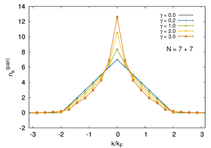
From this expression, we observe that, for spin-balanced systems, the pair-momentum distribution assumes a global maximum for (see also Fig. 5). Phenomenologically, this implies that removing an on-site pair with zero momentum is most favorable. This observation is in line with standard BCS theory where pairing of spin-up and spin-down fermions both located on the Fermi surface but with opposite momenta is most favorable in the presence of an infinitesimally weak but finite attractive coupling, eventually leading to a destabilization of the Fermi surfaces.
We note that, for spin-imbalanced systems, the pair-momentum distribution of the non-interacting system remains constant up to momenta and then decreases monotonically, where LOFF refers to Larkin, Ovchinnikov, Fulde, and Ferrell Fulde and Ferrell (1964); Larkin and Ovchinnikov (1964). For interacting spin-imbalanced systems, the pair-momentum distribution has even been found to develop maxima at , see Refs. Casula et al. (2008); Lee and Guan (2011). Since is associated with the center-of-mass momentum of the formed on-site pairs, the observation of such maxima may be viewed as a precursor for the formation of LOFF-type ground states, where sets the scale for the periodic structure of the ground state in the many-body phase diagram Fulde and Ferrell (1964); Larkin and Ovchinnikov (1964). A priori, however, the mere existence of such maxima in the pair-correlation function does not necessarily entail that pairs with momenta describe the lowest-lying two-body states in the spectrum and that a condensate is formed out of these states, see, e.g., Ref. Roscher and Braun (2016). Still, (pronounced) maxima at may be viewed as an indication that the formation of pairs with momenta is favored.
In Fig. 5, as a concrete example for the pair-momentum distribution, we show our results for as a function of the momentum for a spin-balanced system of fermions. For increasing coupling , we observe that the pair-momentum distribution progressively narrows, resulting in an increase of the maximum at vanishing momenta. This may be viewed as an indicator that pre-formed on-site pairs are favored to occupy the state of zero center-of-mass momentum. Indeed, we do not expect the formation of an inhomogeneous (LOFF-type) ground state for the spin-balanced Fermi gas studied in this work.
Finally we note that the observed progressive formation of a narrow maximum in the momentum distribution associated with the formation of on-site pairs is also consistent with the observation that the system is expected to undergo a smooth crossover from Cooper pairing at small attractive couplings to a gas of bosonic molecules at , see our discussion above.
III.4 Particle-partition entanglement
Knowledge of the one- and two-body density matrices, as presented above, enables the calculation of the particle-partition entanglement entropy. In this section, we show the evolution, with particle number, of the one-particle bipartite entanglement entropy. We define the -particle Rényi entanglement entropy via
| (24) |
where is typically an integer but could in principle take any value in between. The limit yields the von Neumann version of the entanglement entropy:
| (25) |
In this work we will focus on , as higher-particle density matrices become progressively noisier (and therefore more challenging to calculate stochastically) as is increased.
| 0.2 | 0.0011(9) | 0.0003(4) |
|---|---|---|
| 1.0 | 0.06(1) | 0.022(4) |
| 2.0 | 0.257(9) | 0.123(7) |
| 3.0 | 0.51(2) | 0.30(2) |
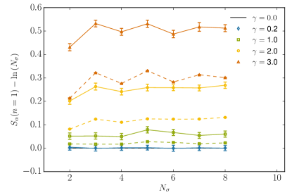
In Fig. 6, we show our results for the von Neumann entropy and the second Rényi entropy at as a function of . For the non-interacting case, we compare with the answer for spinless fermions Barghathi et al. (2017); *PhysRevA.78.042326 and find a similar behavior for very weakly coupled systems. Our results for the strongly interacting case show mild oscillations as a function of relative to the law obeyed by the noninteracting case. However, recall that our results for small even values of are contaminated with contributions that break translation invariance due to the presence of the boundaries.
To characterize the next-to-leading order behavior, a finite-size scaling law for fermions was proposed for in Ref. Barghathi et al. (2017); *PhysRevA.78.042326:
| (26) |
with . Our QMC calculations agree very well with this form, which further confirms the derivations of Ref. Barghathi et al. (2017). Dropping higher-order corrections in Eq. (26), we estimate the -independent offsets for and by fitting our numerical data for the respective entropies to the scaling law (26). The results for the -independent offsets for different values of the coupling can be found in Tab. 2. Note that the one-body density matrix narrows progressively such that with increasing coupling. As can be seen in Tab. 2, becomes larger relative to the non-interacting system for increasing coupling which may be traced back to the dominance of the diagonal elements of the one-body density matrix in this case. In other words, the entropies increase by interaction effects. Within our accuracy, the next-to-next-to-leading order corrections are not resolved, see also Fig. 6.
The procedure to obtain the uncertainties associated with our results for the entanglement entropy was carried out in a specifically designed way, as the diagonalization of the one-body density matrix makes error propagation cumbersome and generally unreliable. The procedure we utilized instead consisted of taking samples of the one-body density matrix around its QMC average with the associated statistical uncertainty (assumed to be gaussian), and then calculating the entanglement entropy for every sample so obtained. Averaging over those samples allowed us to estimate the statistical uncertainties propagated from the one-body density matrix to the entanglement entropies.
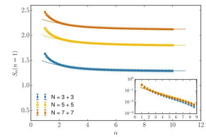
In Fig. 7, we present our results for as a function of for fixed particle numbers at and fixed partition . As in calculations of spatial entanglement in higher dimensions Porter and Drut (2016), we find that the large- limit of is reached rather quickly, as the variation between and is within of the value at for every case we explored. In fact, we observe an exponential decay of the form
| (27) |
which can be appreciated in the inset of Fig. 7.
IV Conclusions
Motivated by experimental and computational advances, we continued here our lattice QMC benchmarking of Fermi gases in 1D. Specifically, we applied lattice QMC methods to the calculation of the one-body density matrix and the associated single-particle momentum distribution, as well as the pair-correlation function and its associated momentum distribution. From the single-particle momentum distribution, we extracted estimates for the speed of sound as well as Tan’s contact. We studied systems at a fixed lattice size of and presented results for systems with varying particle content across a wide range of attractive couplings. We found that systems with small, even particle numbers per species display significant finite-size effects. This can be traced back to the fact that the ground state in this case breaks translation invariance in a periodic box, unlike systems with odd particle numbers per species. The latter appear to converge rapidly to the thermodynamic limit.
In general, our results are in line with earlier studies of two-component gases of fermions in 1D with an attractive contact interaction between the components. In particular, we have illustrated the excellent agreement of our results for the ground-state energy with the exact results from the Bethe ansatz. Moreover, we have found very good agreement for the contact parameter calculated differently in a previous study Rammelmüller et al. (2015). Even more, our first comparatively crude estimates for the speed of sound are in accordance with the well-known exact results of this quantity Krivnov and Ovchinnikov (1965); Lieb and Liniger (1963); Fuchs et al. (2004). Also in accordance with previous studies Fuchs et al. (2004); Wadati and Iida (2007), we find that, in the weakly-coupled regime with , the calculated correlation functions, and therefore also the momentum distributions, are still well approximated by the ones of the non-interacting system. The dynamics in this regime still appears to be dominated by the presence of the Fermi points. In the strongly-coupled regime with , we then find that the single-particle momentum distributions start to flatten out and the pair-momentum distribution develops a pronounced maximum at vanishing pair momentum relative to the corresponding distribution of the non-interacting system. Our estimates for the sound velocity reveal that the system undergoes a crossover from the weakly-coupled regime, where the sound velocity remains close to the Fermi velocity, to a strongly-coupled regime for , where the sound velocity drops drastically. In detailed analytic studies of the many-body phase diagram Lieb and Liniger (1963); Krivnov and Ovchinnikov (1965); Fuchs et al. (2004); Wadati and Iida (2007), this behavior was traced back to the fact that the dynamics of the system is governed by Cooper-type pairing in the weak-coupling limit and by the formation of tight bosonic molecules in the strong-coupling limit.
Finally, we have used our results for the one-body density matrix to provide testable predictions for the Rényi and von Neumann particle partition entanglement entropies for a partition of particles. Our calculations, for varying couplings, orders , and total particle numbers , display a logarithmic growth with and mild oscillations on top of that growth, which further confirms the results of recent analytic studies. Additionally, we explored the -dependence of for several and found that it decays exponentially to the limiting value with an approximately -independent decay amplitude and rate.
One of the goals of the present work is to benchmark our lattice QMC approach for the computation of ground-state properties with known exact results. Indeed, we have found very good agreement with the exact results for the observables considered here. Our present study therefore sets the methodological stage for future studies of correlation functions of Fermi gases in higher dimensions, where exact results for, e.g., correlation functions, are urgently needed. In particular, for studies of systems with a finite spin- and mass-imbalance, the computation of general correlation functions is of interest as the formation of an inhomogeneous (LOFF-type) ground state is expected to leave its imprint on these quantities.
Acknowledgments.– J.B. and L.R. are grateful to H.-W. Hammer and A. Volosniev for useful discussions and are grateful to A. Volosniev for comments on the manuscript. This work was supported by HIC for FAIR within the LOEWE program of the State of Hesse. Moreover, this material was based upon work supported by the National Science Foundation under Grant No. PHY1452635 (Computational Physics Program).
Appendix A Systematics
In this appendix we discuss the behavior of our results as a function of the lattice size and the imaginary projection time . Although, in principle, one should compute quantities in the limit of infinite and to guarantee full convergence to the respective physical limit, it is often sufficient to carry out calculations at finite, but large, parameter values, as shown below. Comparisons between different systems are shown for a representative system with particles with strong and weak interactions. As mentioned in the main text, the shown error bars reflect statistical uncertainties of samples. The associated typical autocorrelation times for the energy are of the order of . In our discussion below, decorrelation between points at different in the momentum distribution is tacitly assumed. However, an explicit detailed analysis of the autocorrelation times for this quantity has not been performed and therefore the true error bar on the results may be (slightly) underestimated as the autocorrelation time may have been underestimated for this quantity.
A.1 Finite lattice size
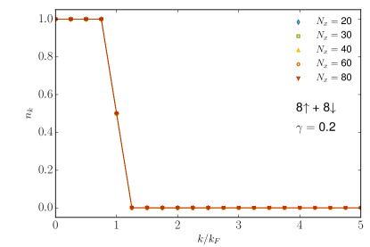
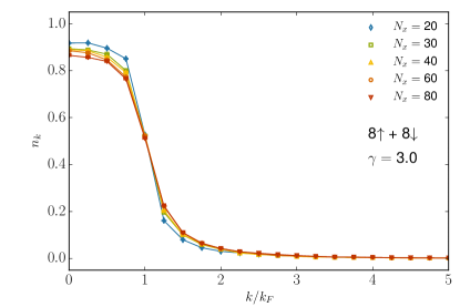
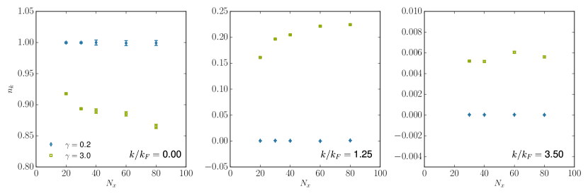
In the present work, we employ periodic boundary conditions in our calculations. We shall now address the effect of finite lattice sizes in case of such boundary conditions in order to have a more complete overview of possible systematic errors. To this end, we exploit the fact that, in the infinite-volume limit, physical observables555More precisely, observables rendered dimensionless with suitably chosen powers of the density (or, equivalently, the Fermi momentum). should only depend on the value of the dimensionless coupling . This implies that our results for a given fixed value of the dimensionless coupling should not exhibit an explicit dependence on the density , if the box size has been chosen sufficiently large. In the top panels of Fig. 8, we show the momentum distribution for lattice sizes of , and for fixed and . Recall that where is the lattice spacing. In the bottom panels of Fig. 8, we illustrate the scaling behavior of with the lattice size for (from left to right), again for fixed and . We clearly observe that weakly coupled systems, exemplified by the momentum distribution with , show a indiscernible dependence on the lattice size and therefore associated errors are almost absent, as evident from Fig. 8. For the strongly coupled case at , finite-size effects are more pronounced, most prominently for momenta close to the Fermi point . However, even close to the Fermi point, the volume dependence is already very weak for . Given these results, we do not employ an extrapolation to the infinite-volume limit but consider to be sufficiently converged, which is therefore the value used throughout this work.
Obviously, the momentum distribution is not the only quantity influenced by finite-size effects. Our results for the one- and two-body density matrices, however, feature the same type of convergence and will not be considered separately at this point. We add that we also find agreement with previous studies of the ground-state energy in 1D Rammelmüller et al. (2015).
A.2 Finite imaginary time
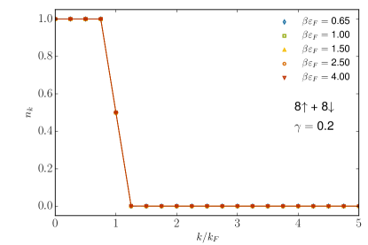
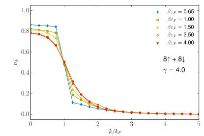
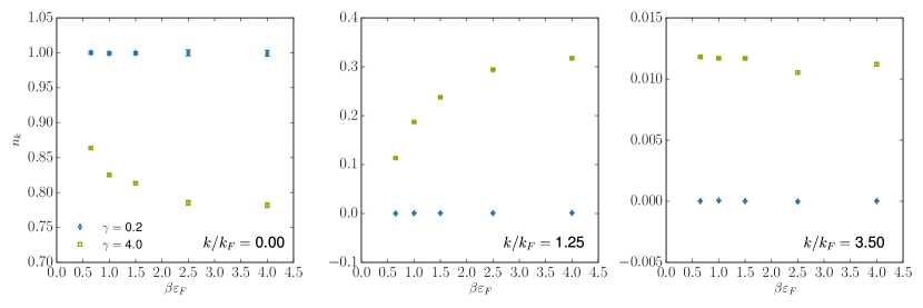
As mentioned in the text, we evaluate the projection up to a finite value of , corresponding to a finite effective inverse temperature. Since our approach exploits an initial guess state (in our case taken to be a Slater determinant) and projects to the ground-state, we need to make sure that the obtained results are fully converged to the limit . In Fig. 9, we show this effect for two systems in the weakly and strongly interacting regime. Again, as expected, the essentially free case at shows no dependence on and is converged almost immediately, see also the bottom panels of Fig. 9 where is shown as a function of . For strongly interacting systems, larger projection times are required to observe convergence. As depicted in the bottom panels of Fig. 9, we observe that the dependence on starts to become weak for , even for the most strongly coupled systems considered in this work. Therefore, we have not employed an extrapolation to infinite but have rather used to obtain the results presented in the main part of this work.
References
- Bloch et al. (2008) I. Bloch, J. Dalibard, and W. Zwerger, Rev. Mod. Phys. 80, 885 (2008).
- Haller et al. (2010) E. Haller, M. J. Mark, R. Hart, J. G. Danzl, L. Reichsöllner, V. Melezhik, P. Schmelcher, and H.-C. Nägerl, Phys. Rev. Lett. 104, 153203 (2010).
- Liao et al. (2010) Y.-a. Liao, A. S. C. Rittner, T. Paprotta, W. Li, G. B. Partridge, R. G. Hulet, S. K. Baur, and E. J. Mueller, Nature 467, 567 (2010).
- Wu and Thomas (2012) H. Wu and J. E. Thomas, Phys. Rev. Lett. 108, 010401 (2012).
- Guan et al. (2013) X.-W. Guan, M. T. Batchelor, and C. Lee, Rev. Mod. Phys. 85, 1633 (2013), arXiv:1301.6446 [cond-mat.quant-gas] .
- Voit (1995) J. Voit, Rep. Prog. Phys. 57, 977 (1995).
- Schollwöck (2005) U. Schollwöck, Rev. Mod. Phys. 77, 259 (2005).
- Sowiński et al. (2013) T. Sowiński, T. Grass, O. Dutta, and M. Lewenstein, Phys. Rev. A 88, 033607 (2013).
- Sowiński et al. (2015) T. Sowiński, M. Gajda, and K. Rzażewski, EPL (Europhysics Letters) 109, 26005 (2015).
- Pęcak and Sowiński (2016) D. Pęcak and T. Sowiński, Phys. Rev. A 94, 042118 (2016).
- Lindgren et al. (2014) E. J. Lindgren, J. Rotureau, C. Forssén, A. G. Volosniev, and N. T. Zinner, New Journal of Physics 16, 063003 (2014).
- Grining et al. (2015) T. Grining, M. Tomza, M. Lesiuk, M. Przybytek, M. Musiał, P. Massignan, M. Lewenstein, and R. Moszynski, New Journal of Physics 17, 115001 (2015).
- Rammelmüller et al. (2015) L. Rammelmüller, W. J. Porter, A. C. Loheac, and J. E. Drut, Phys. Rev. A 92, 013631 (2015).
- Loheac et al. (2015) A. C. Loheac, J. Braun, J. E. Drut, and D. Roscher, Phys. Rev. A 92, 063609 (2015), arXiv:1508.03314 [cond-mat.quant-gas] .
- Bethe (1931) H. Bethe, Zeitschrift für Physik 71, 205 (1931).
- Casula et al. (2008) M. Casula, D. M. Ceperley, and E. J. Mueller, Phys. Rev. A 78, 033607 (2008).
- Lee and Guan (2011) J. Y. Lee and X. W. Guan, Nucl. Phys. B853, 125 (2011).
- Roscher and Braun (2016) D. Roscher and J. Braun, (2016), arXiv:1611.02081 [cond-mat.quant-gas] .
- Wenz et al. (2013) A. N. Wenz, G. Zürn, S. Murmann, I. Brouzos, T. Lompe, and S. Jochim, Science 342, 457 (2013), arXiv:1307.3443 [cond-mat.quant-gas] .
- Zürn et al. (2013) G. Zürn, A. N. Wenz, S. Murmann, A. Bergschneider, T. Lompe, and S. Jochim, Phys. Rev. Lett. 111, 175302 (2013), arXiv:1307.5153 [cond-mat.quant-gas] .
- Zinner (2016) N. T. Zinner, EPJ Web of Conferences 113, 01002 (2016), arXiv:1510.03619 [quant-ph] .
- Braun et al. (2005) J. Braun, B. Klein, and H. J. Pirner, Phys. Rev. D72, 034017 (2005), arXiv:hep-ph/0504127 [hep-ph] .
- Berger et al. (2015) C. E. Berger, E. R. Anderson, and J. E. Drut, Phys. Rev. A 91, 053618 (2015), arXiv:1410.8103 [cond-mat.quant-gas] .
- Berger et al. (2016) C. E. Berger, J. E. Drut, and W. J. Porter, Comput. Phys. Commun. 208, 103 (2016), arXiv:1510.02976 [cond-mat.quant-gas] .
- Hueck et al. (2017) K. Hueck, N. Luick, L. Sobirey, J. Siegl, T. Lompe, and H. Moritz, (2017), arXiv:1704.06315 .
- McKenney et al. (2016) J. R. McKenney, C. R. Shill, W. J. Porter, and J. E. Drut, J. Phys. B 49, 225001 (2016), arXiv:1510.08503 [cond-mat.quant-gas] .
- Amico et al. (2008) L. Amico, R. Fazio, A. Osterloh, and V. Vedral, Rev. Mod. Phys. 80, 517 (2008), arXiv:quant-ph/0703044 [quant-ph] .
- Horodecki et al. (2009) R. Horodecki, P. Horodecki, M. Horodecki, and K. Horodecki, Rev. Mod. Phys. 81, 865 (2009).
- Eisert et al. (2010) J. Eisert, M. Cramer, and M. B. Plenio, Rev. Mod. Phys. 82, 277 (2010).
- Haque et al. (2009) M. Haque, O. S. Zozulya, and K. Schoutens, Journ. Phys. A 42, 504012 (2009).
- Zozulya et al. (2007) O. S. Zozulya, M. Haque, K. Schoutens, and E. H. Rezayi, Phys. Rev. B 76, 125310 (2007).
- Haque et al. (2007) M. Haque, O. Zozulya, and K. Schoutens, Phys. Rev. Lett. 98, 060401 (2007).
- Zozulya et al. (2008) O. S. Zozulya, M. Haque, and K. Schoutens, Phys. Rev. A 78, 042326 (2008).
- Barghathi et al. (2017) H. Barghathi, E. Casiano-Diaz, and A. Del Maestro, (2017), arXiv:1703.10587 [cond-mat.quant-gas] .
- Yang (1967) C. N. Yang, Phys. Rev. Lett. 19, 1312 (1967).
- Gaudin (1967) M. Gaudin, Physics Letters A 24, 55 (1967).
- Barlette et al. (2000) V. E. Barlette, M. M. Leite, and S. K. Adhikari, Eur. Phys. J. 21, 435 (2000), quant-ph/0012087 .
- Luttinger (1963) J. M. Luttinger, Journ. Math. Phys. 4, 1154 (1963).
- Drut (2012) J. E. Drut, Phys. Rev. A 86, 013604 (2012).
- Rammelmüller et al. (2016) L. Rammelmüller, W. J. Porter, and J. E. Drut, Phys. Rev. A 93, 033639 (2016).
- Wadati and Iida (2007) M. Wadati and T. Iida, Phys. Lett. A 360, 423 (2007).
- Tracy and Widom (2016) C. A. Tracy and H. Widom, ArXiv e-prints (2016), arXiv:1609.07793 [math-ph] .
- Griffiths (2004) D. J. Griffiths, Introduction to Quantum Mechanics (Prentice Hall International, 2004).
- Girardeau (1960) M. Girardeau, Journ. Math. Phys. 1, 516 (1960), http://dx.doi.org/10.1063/1.1703687 .
- Lieb and Liniger (1963) E. H. Lieb and W. Liniger, Phys. Rev. 130, 1605 (1963).
- Lieb (1963) E. H. Lieb, Phys. Rev. 130, 1616 (1963).
- Krivnov and Ovchinnikov (1965) V. Krivnov and A. Ovchinnikov, Sov. Phys. JETP 40, 781 (1965).
- Fuchs et al. (2004) J. N. Fuchs, A. Recati, and W. Zwerger, Phys. Rev. Lett. 93, 090408 (2004), cond-mat/0402448 .
- Kemler et al. (2017) S. Kemler, M. Pospiech, and J. Braun, J. Phys. G 44, 015101 (2017), arXiv:1606.04388 [nucl-th] .
- Luther and Peschel (1974) A. Luther and I. Peschel, Phys. Rev. B 9, 2911 (1974).
- Haldane (1981) F. D. M. Haldane, Phys. Rev. Lett. 47, 1840 (1981).
- Cazalilla (2004) M. A. Cazalilla, Journ. Phys. B 37, S1 (2004), cond-mat/0307033 .
- Giorgini et al. (2008) S. Giorgini, L. P. Pitaevskii, and S. Stringari, Rev. Mod. Phys. 80, 1215 (2008).
- Barth and Zwerger (2011) M. Barth and W. Zwerger, Annals of Physics 326, 2544 (2011), arXiv:1101.5594 [cond-mat.quant-gas] .
- Tan (2008a) S. Tan, Annals of Physics 323, 2952 (2008a).
- Tan (2008b) S. Tan, Annals of Physics 323, 2971 (2008b).
- Tan (2008c) S. Tan, Annals of Physics 323, 2987 (2008c).
- Drut et al. (2011) J. E. Drut, T. A. Lähde, and T. Ten, Phys. Rev. Lett. 106, 205302 (2011).
- Fulde and Ferrell (1964) P. Fulde and R. A. Ferrell, Phys. Rev. 135, A550 (1964).
- Larkin and Ovchinnikov (1964) A. Larkin and Y. Ovchinnikov, Zh.Eksp.Teor.Fiz. 47, 1136 (1964).
- Porter and Drut (2016) W. J. Porter and J. E. Drut, Phys. Rev. B 94, 165112 (2016).
