The Weak Null Condition and Kaluza-Klein Spacetimes
Zoe Wyatt
School of Mathematics
The University of Edinburgh
James Clerk Maxwell Building
Peter Guthrie Tait Road
Edinburgh
EH9 3FD
United Kingdom
zoe.wyatt@ed.ac.uk
Abstract.
In this paper we prove the non-linear stability of a system of non-linear wave equations satisfying the weak null condition. In particular, this includes the case of the non-linear stability of Minkowski spacetime times a -torus subject to perturbations depending only on the non-compact coordinates. Our argument very closely follows the proof of the non-linear stability of Minkowski spacetime by Lindblad and Rodnianski [14].
1. Introduction
Theories of higher-dimensional gravity are of great interest to string theorists. Some of these additional dimensions are typically compactified in order for these theories to reflect the perceived dimensional universe. One such theory is that of Kaluza-Klein, where, in the simplest case, dimensional gravity is compactified on a circle to obtain at low energies a dimensional coupled Einstein-Maxwell-Scalar system, see (2.6). In an influential work by Witten, it was shown that Kaluza-Klein theory is unstable at the semiclassical level and heuristic arguments were given for classical stability [18]. In this paper we rigorously prove the classical stability against perturbations depending only on the non-compact coordinates. The precise details are given in Theorem 2.1, but the main idea is the following:
Theorem 1.1.
The Minkowski vacuum of the Einstein-Maxwell-Scalar system arising from the zero modes of dimensional pure Einstein theory compactified on a is non-linearly stable. Furthermore, the radii of the are non-linearly stable to peturbations of the zero modes.
To compare Theorem 1.1 with the instability in [18], recall that Witten’s classical solution, which indicated the semiclassical instability of Kaluza-Klein in the case , had initial data with topology . This initial data cannot be imposed on the Kaluza-Klein spacetime, but rather is conjectured to appear spontaneously from a quantum-mechanical process. There is no smooth perturbation of any size, let alone of the small size we consider, that could lead to a change in the topology of our initial data. Thus the two results do not disagree.
The non-linear stability we consider is subject to the symmetry assumption that the perturbations only depend on the non-compact directions. This symmetry assumption, also called the zero mode truncation, is, in the physics literature, called consistent since it yields solutions of the full equations of motion of the higher dimensional theory. Indeed initial data obeying this symmetry will yield a solution similarly invariant in the compact directions.
As frequently done from an effective theory point of view, one can further make a heuristic physical argument that for sufficiently small initial compact radii, it is in fact sufficient to only consider zero mode perturbations [16]. Our result shows that the radii are non-linearly stable to zero mode perturbations. Of course from the non-linear PDE point of view, the dynamics from the non-zero modes are still relevant and remain to be understood. Nonetheless, stability of the zero modes is a necessary first step. We now introduce the PDE, see Section 2 for further discussion on this application to Kaluza-Klein.
The vacuum Einstein equations
determine the evolution of a Lorentzian spacetime . The initial data for these equations consists of Cauchy 3-surface with metric and a symmetric 2-tensor , such that the constraint equations hold on
(1.1)
Here is the Levi-Civita connection of .
One further requires an embedding such that the pull-back of the solution to is and is the second fundamental form of .
It was shown by Choquet-Bruhat and Geroch that for any smooth initial data satisfying the constraint equations there exists a maximal, unique up to diffeomorphism, globally-hyperbolic spacetime that is the Cauchy development of the initial data and that satisfies the vacuum Einstein equations [3].
A natural question to then ask is whether the simplest solution of the vacuum Einstein equations, the Minkowski spacetime, is stable to small perturbations of the initial data . This question of the non-linear stability of Minkowski spacetime and the geodesic completeness of the perturbed solution was first shown in the monumental work by Christodoulou and Klainerman [4].
However their proof, and gauge choice, differed significantly from the first proof of local well-posedness by Choquet-Bruhat [6]. In this paper, Choquet-Bruhat fixed the coordinate invariance by choosing wave coordinates which are defined to satisfy the covariant wave equation
where is the Levi-Civita connection of . Relative to these wave coordinates the metric satisfies the wave-coordinate condition
(1.2)
This condition is also known as the harmonic, de Donder, or wave gauge. In this gauge, the Einstein equations reduce to a system of non-linear wave equations
(1.3)
where is an inhomogeneity we will discuss shortly. Here is the reduced wave operator. Although the local well-posedness of the system (1.3) was shown in [6], for a long time it was believed that a global-in-time solution could not be achieved [1].
Nonetheless as shown in the seminal work by Lindblad and Rodnianski, it is in fact possible to use the wave gauge to prove the non-linear stability of Minkowski by treating the system (1.3) using an energy argument at the level of the metric tensor [13, 14].
Our proof very closely follows [14] and we refer to it for a more detailed discussion on the literature and motivation behind their proof.
We now briefly summarise the result of [14]. The Einstein equations (1.3) in wave coordinates coupled to a scalar field, written in terms of the perturbation away from Minkowski , take the form
(1.4a)
where the inhomogeneity is
(1.4b)
Note the term involving in (1.4a) comes from adding a stress energy tensor to the Einstein equations in the form .
Here is a linear combination of the standard quadratic null forms
(1.5)
whose behaviour has been studied for some time, see [8], [9] and [5]. Most importantly both null forms can be estimated by
(1.6)
where are all space-time derivatives and denotes derivatives tangent to the light cones.
is a term quadratic in with coefficients that smoothly depend on such that . Furthermore define and throughout this paper we will raise and lower indices with respect to the background Minkowski metric .
The structure of the non-linearity in (1.4), in particular that of the quadratic non-null form , was exploited to great effect in [14], see also our later Section 2.2 on the weak null condition.
Furthermore to deal with the ADM mass term at spatial infinity, Lindblad and Rodnianski defined a cut-off function by
(1.7)
and a 2-tensor in terms of the ADM mass by
(1.8)
Lindblad and Rodnianski showed that for smooth initial data , sufficiently ‘close’ to Minkowski initial data, satisfying the constraint equations,
the solution to (1.4) can be extended to a global-in-time solution. We will discuss this notion of ‘closeness’ to Minkowski initial data shortly.
Note here is the covariant derivative associated to .
In this work we consider the unknowns
(1.9a)
for some , satisfying the following generalised PDE system:
(1.9b)
together with the wave-coordinate condition
(1.9c)
The quadratic terms are linear combinations of the null forms (1.5) in terms of variables, contracting the arguments of the null forms with and/or arbitrary as appropriate.
The remaining non-null terms are of the form
(1.9d)
Here are some arbitrary constant coefficients and are terms quadratic in with coefficients smoothly dependent on such that . Although we have added additional non-linearities to both the and terms, we have specifically only added terms which are null forms to . This choice is so that the variables obey the same estimates as the ‘best’ components of . See also Remark 5.8.
To discuss the initial data for this system further, introduce the Minkowski conformal vector fields
and the standard multi-index notation
The initial data consists of the collection where is a 3-dimensional Riemannian manifold, a symmetric 2-tensor and are smooth functions. We assume that the initial surface is diffeomorphic to , has ADM mass , and that there exists a global coordinate chart on such that as the initial data satisfies
(1.10)
For and fixed constant , define an initial weighted energy by
(1.11)
where the weight function is defined as
(1.12)
Here is a constant to be fixed later.
Just as for the initial data (1.8), we follow Lindblad and Rodnianski and deal with the ADM mass at spatial infinity by defining the 2-tensor
This is also depicted in Figure 1 on page 1. The weighted energy for the solution is defined as
(1.13)
where the unknown dynamical variables are
Our main result is now:
Theorem 1.2.
Let be smooth initial data for (1.9), asymptotically flat in the sense of (1.10), with diffeomorphic to .
There exists a constant such that for all and initial data such that
the solution to the system (1.9) can be extended to a global-in-time smooth solution, agreeing with the initial data on
and for which the energy satisfies the following inequality for all time
(1.14)
Similar to the method used in [14], the proof of Theorem 1.2 relies on a ‘bootstrap’ assumption to make a continuous induction argument .
By standard theory of non-linear wave equations, we can obtain a local-in-time smooth solution of our PDE obeying the wave-gauge condition in some maximum interval . This maximum time of existence is defined by the blow-up of the energy: as .
Furthermore the smallness condition on implies that there is some maximal time on which the following inequality holds
(1.15)
where is some fixed constant with . The aim of the proof is to contract on the bootstrap assumption (1.15) by choosing sufficiently small. That is, we show that
(1.16)
By choosing sufficiently small, this will imply
Since is continuous and we have contracted the bootstrap condition, cannot have been the maximal time for which (1.15) holds, and so we must have . This however would then imply that is finite, and so we may extend the solution beyond . This contradicts the maximality of and so we have a global-in-time solution with . Thus the aim of our paper is to show (1.14).
1.1. Structure of the Paper
First in Section 2 we discuss the motiving example from Kaluza-Klein theory, the Weak Null condition and some other literature. In Section 3 we set up the null frame, and in Section 4 we discuss the generalised PDE system (1.9) and its form when written with respect to this null frame. Section 5 is where we derive estimates coming from the wave coordinates and then apply these to the inhomogeneity. In Sections 6 and 7 we derive the main decay estimates which are then used to derive an integrated energy inequality in Section 8 which concludes our proof of (1.16). In Appendix A we derive the non-minimally coupled Einstein-Maxwell-Scalar system, which gives a slightly different approach to the higher dimensional system discussed so far and in Section 2. In Appendix B we state some useful identities from [14].
2. Zero Mode Reduction of Kaluza Klein
The motivation for considering the system (1.9) is to prove Theorem 1.1, and we now discuss how this is achieved. For simplicity, we first consider a dimensional gravitational theory compactified on a circle . This was the original set-up considered by Klein [10] using previous work by Kaluza [7]. Let the dimensional metric have indices and satisfy the vacuum Einstein equations
(2.1)
Written with respect to the wave-coordinate condition on the full dimensional metric, the equation of motion (2.1) becomes a non-linear wave equation
(2.2)
Let , for , denote the coordinates of the non-compact spacetime and denote the coordinate of the fifth compact dimension. Since is compact, say of radius , we can Fourier expand the metric
(2.3)
If we substitute the expansion (2.3) into the left-hand-side of (2.2) and look at just the terms coming from the flat background we obtain
Heuristically one can see that the modes with , will satisfy non-linear Klein-Gordon equations with mass . At this point, the standard physical argument is to ignore these modes by taking sufficiently small that the mass is larger than any probable energy [16].
From the PDE point of view, including the modes will lead to terms of the form
and thus to the trapping of energy in the compact direction, a much more difficult problem for future work.
Hence we consider only the modes by setting for all . This implies the higher-dimensional metric depends only on the non-compact coordinates
(2.4)
Assuming the flat, background metric on , this condition is equivalent to constraining the perturbations to satisfy
Indeed under the assumption (2.4), it is standard, see for example [16], to use an Ansatz involving the dimensional metric , dilaton and vector potential
(2.5)
where are some constants. Indeed provided this choice fully parametrises the higher-dimensional metric. Using this Ansatz, the higher-dimensional vacuum Einstein equations (2.1) reduce to the following non-minimally coupled111We use ‘non-minimal’ here and throughout in the sense that there is non-trivial coupling between the scalar and Maxwell fields. -dimensional Einstein-Maxwell-Scalar system:
(2.6a)
(2.6b)
(2.6c)
where .
The Ansatz (2.5) is chosen so that , and transform as a dimensional metric, vector potential and scalar field respectively. A similar argument can be made when , see Appendix A.
Indeed when we compactify over a , not merely an , there will be additional compact coordinates where . While the non-linearities in (2.6) may exhibit some, perhaps mixed, structure involving null and non-null terms, much more is known about the non-linear structure at the level of the higher-dimensional metric and so this is what we turn to now. Impose the flat, background metric on given by
We use Roman letters on the dimensional non-compact space, underlined Roman letters on the -dimensional compact space and Greek letters for the full dimensional space. Note the choice of flat metric implies
Let us now turn to the PDE system assuming (2.7). If the initial data satisfies (2.4), and the PDE is invariant in the compact directions, then the solution will be also.
The perturbation and inverse perturbation are defined by
where . Differentiating this identity and using (2.7) implies .
Imposing the wave coordinate condition (1.2) on the full metric ,
(2.8a)
the vacuum Einstein equations reduce to the following non-linear wave system
(2.8b)
where the non-null terms are
(2.8c)
As before, consists of linear combinations of the standard null-forms (1.5), and is quadratic in and vanishing when . The explicit equations are given in Proposition 4.1. If we consider the unknowns as variables then the system (2.8) falls into the class considered in (1.9). Using Theorem 1.2 we now obtain the following.
Theorem 2.1.
Let be smooth initial data for the equations of motion (2.8) arising from the dimensional vacuum Einstein equations under (2.7). Define and the 2-tensor by
with defined in (1.7) and .
Suppose also that is diffeomorphic to and the initial data satisfies the constraint equations (1.1) and is asymptotically Kaluza-Klein in the sense that
(2.9)
Furthermore for and define
Then there exists a constant such that for all and initial data with , the solution
to (2.8) exists for all times and
in particular as . Hence the perturbed radii decay to the radii of the background geometry.
We assume the initial data required by Theorem 2.1 exists, however the constraint equations have a perhaps more natural interpretation from the perspective of the dimensional non-minimally coupled Einstein-Maxwell-Scalar system (A.4). See Appendix A for more details. Note also that the radii of the in the background geometry do not necessarily have to be taken small, merely non-zero.
In fact, in an earlier work by Lindblad and Rodnianski, it was shown that the perturbed solution gives a future geodesically complete manifold.
Since our variables obey the same decay rates, it should follow similarly to Section 16 in [13] that the perturbed solution yields a future causally geodesically complete solution asymptotically converging to .
2.1. Other results and future work
We now make some final comments on the additional terms considered in the generalised system (1.9). Although our method of proof follows from [14], the terms and cannot be treated directly as variables in the original system (1.4) of Lindblad and Rodnianski.
For one, these variables have non-trivial inhomogeneities which is unlike those presented in (1.4). In the Kaluza-Klein example there is also a physical interpretation. Equation (2.8c) includes a term of the form
This describes interactions between the dimensional metric and the scalar fields . Similar terms exist in and also. This non-trivial coupling cannot come from the stress-energy tensor of a massless scalar field, and so the more general PDE system (1.9) is required.
The method of Lindblad and Rodnianski has also been used by Choquet-Bruhat, Loizelet and Chrusciel to show the non-linear stability of Minkowski spacetime for [2]. Indeed following the method of [14], Loizelet proved in [15] that the Minkowski solution minimally coupled to the Maxwell equations is non-linearly stable. The system considered was:
(2.10)
Using the wave-coordinate condition (1.2) and the Lorenz gauge this PDE reduces to a system of the form
(2.11)
The PDE (2.11) has very similar properties to our general PDE (1.9), see Remark 5.8 for more details. Furthermore (2.6) would reduce to (2.10) if could be set to a constant, thus unifying gravity and electromagnetism from a pure higher-dimensional gravity. However the equation of motion (2.6c) for is not a free wave equation, but rather has an inhomogeneity involving . From this one sees that it is inconsistent to simply take , since this Ansatz would not satisfy the equations of motion. Thus our more generalised system (1.9) is needed to treat (2.6). This should be contrasted with our earlier Ansatz that for all . This does not violate the equations of motion and thus gives what is often called a consistent truncation.
Of course not all Einstein systems fall into the class considered in (1.9). An example is general relativity coupled to non-linear electromagnetic fields, such as the Born-Infeld system, considered in [17].
An obvious question not answered in our work is to consider all modes not just the mode. Furthermore one could ask whether other product spacetimes of interest in string theory, such as where is a Calabi-Yau manifold, are non-linearly stable against some, or all, perturbations of initial data. In the full mode case the non-linear wave equations contain Klein-Gordon terms, which have only recently been treated at the full non-linear level by [11].
2.2. The Weak Null Condition
As alluded to so far, there are important properties of a non-linearity which imply, or at least allow one to hope, that a PDE may be solved globally. One such condition on the non-linearities is the weak null condition, first introduced by Lindblad and Rodnianski in [12]. Their idea was to look at an asymptotic form of the PDE and determine whether this has global solutions. Here we just state the condition following the notation of the original work, but for more details and motivation see [12, 14].
Definition 2.2.
Consider a system of hyperbolic PDEs for unknowns
(2.12)
where vanishes to third order as and unless and . Note also are multi-indices, not coordinate indices.
Take the following asymptotic expansion
(2.13)
as and in the wave-zone region .
Equating terms of order gives the system
(2.14)
where
The system (2.12) is said to satisfy the weak null condition if the asymptotic system (2.14) has solutions for all and if the solutions together with their derivatives grow at most exponentially in for all initial data decaying sufficiently fast in .
Note the null-forms (1.5) satisfy a stricter condition called the null condition, analysed by Klainerman in [8], which requires .
At each point introduce the null vectors defined by
In a neighbourhood of each point, we can also find a pair of orthonormal vector fields orthogonal to the null pair . This set is the null frame, see also Section 3 for more details. Let the inverse perturbation be
.
As described in (2.13), we take the asymptotic expansion
and substitute this into the PDE system (1.9) to yield
(2.15a)
(2.15b)
(2.15c)
Here are non-null terms defined in (4.1d) and (2.15c) is the asymptotic form of the wave-coordinate condition (1.2). Following the argument of [12], by (2.15a)
implying is preserved along the integral curves of the vector field and hence (2.15c) is preserved under the flow of (2.15a). Contract (2.15a) with to obtain the equation
which can be solved globally for . Using this solution, one can now solve (2.15b) for . Furthermore by contracting (2.15a) with , for we obtain the equation
This can also be solved globally and thus the only remaining unknown component is . Contracting (2.15a) with gives
Since222See [12] for further discussion here. the RHS does not contain terms, the equation can be solved globally for .
The above argument implies the following proposition:
Proposition 2.3.
The asymptotic system for the PDE (1.9) takes the form (2.15). The solution for this system (2.15) exists globally with all components remaining uniformly bounded while grows at most as . Thus (1.9) satisfies the weak null condition.
Moreover Theorem 1.2 could be seen as an example supporting the conjecture that non-linear wave equations arising from the Einstein equation and wave-coordinate condition that satisfy the weak null conjecture have global-in-time solutions for small data.
where . Note that is tangent to the outgoing Minkowski null cones and is tangent to the ingoing cones .
Furthermore
Locally let be orthonormal smooth vector fields spanning the tangent space of the spheres . Then forms a null frame. Define
Relative to the null frame the Minkowski metric takes the form
where denote any of the vectors and . Since does not admit a global orthonormal frame, we consider the projections of and defined by
If we denote then the set defines a global frame. Furthermore if we define then the set
spans the tangent space of the outgoing light cone. As in [14], define the following notation:
Definition 3.1.
Let
(3.1)
where is the set of null frame vector fields tangent to the outgoing cones.
For any two families and of vector fields and an arbitary 2-tensor , define the following pointwise seminorms
Furthermore for a collection where , let
where is the standard basis on .
4. The (extended) Einstein Equations and Wave Coordinates
In this section we look at the structure of the non-linearity of the PDE (1.9) with respect to the null frame. Recall our unknown variables are
where is the perturbation from the background Minkowski. For small , the inverse perturbation is
where and vanishes to second order at . The PDE, repeated from (1.9), is
(4.1a)
where we defined the non-linearities by
(4.1b)
together with the wave-coordinate condition
(4.1c)
The quadratic terms are linear combinations of the null forms (1.5) in terms of variables, contracting with and/or arbitrary as appropriate. While the remaining non-null terms are of the form
(4.1d)
Again are some arbitrary coefficients.
Lastly the terms and are quadratic forms in , with coefficients depending smoothly on and vanishing for . Note we have used compact notation in (4.1), writing to represent , similarly for and also.
Proposition 4.1.
The mode reduction of Kaluza Klein on a subject to the wave-coordinate condition (1.2) is included in the generalised PDE system (4.1).
Proof.
Under (2.7) and the wave-coordinate condition the vacuum Einstein equations in reduce to the system
(4.2a)
(4.2b)
(4.2c)
The non-linearities are given by
Here indicates the previous bracketed term are repeated with and swapped.
Recall also the indices and are as defined in Section 2. Clearly and are linear combinations of the standard null forms (1.5) and so satisfy the required estimates. If we consider the set then we see the PDE (4.2) falls into the system described in (4.1)
∎
Remark 4.2.
As illustrated in the case in (2.6), the Einstein equation for the higher-dimensional metric can be interpreted from the view of the lower-dimensional theory as a dimensional metric coupled to a Maxwell vector potential and a scalar field.
This structure is reflected in (4.2a), which comes from the non-vacuum dimensional Einstein equation. Up to redefining variables, as done in (2.5), one can heuristically see the coupling between the Maxwell fields , scalar fields and the geometry .
The first term contains the standard non-null expression in (1.4) studied by Lindblad and Rodnianski coming from the self-interaction of the metric.
The term comes from the non-trivial coupling between the background geometry and the scalar fields .
The first term in involves the interactions between the vector potentials, while the second term comes from the stress-energy tensor for a scalar wave.
Next we turn to the structure of the non-linearity of the PDE (4.1) with respect to the null frame.
As in [14], first express the non-linearity in terms of some general tensors and/or scalars. For example, for symmetric 2-tensors we define
Note there are no free indices here. Similar definitions holds for with some arbitrary functions. All together, let
The reason for using this notation is that eventually we will want to calculate where . This notation allows us to derive estimates which still hold even when we have distributed the derivatives across the terms in the non-linearity. See for example Corollary 5.6.
For the null terms, it is irrelevant which components of the unknowns are being considered, but it is crucial which derivatives appear. Thus for some , which are either 2-tensors or scalars as required, define
Let be arbitrary 2-tensors, arbitrary functions and 2-tensors or scalars as required. For the terms contained in (4.1d) we obtain
Proof.
Expanding with respect to the null frame we find
Note that involves . By considering possible indices, we see another possible term is of the form
However this term does not contain and so in we would pick up additional terms of the form which cannot be controlled.
The estimate for comes from the definition of and in (4.1) and estimate (1.6) for null forms.
∎
Remark 4.4.
Our proof follows very closely the proof of [14]. However to be self-contained, this paper repeats several results directly from [14]. Where a result here is given as ‘modified’ from a result in [14], it generally follows from their proofs with at most a very simple calculation difference.
5. Wave Gauge and Estimates of the Inhomogeneity
Recall the definition of the wave-coordinate condition
(5.1)
The following Lemmas exploit to great effect this choice of gauge and properties of the null frame. In particular Lemma 5.1 implies that we can exchange a full derivative on certain ‘good’ components of the metric, with a good derivative on all components of the metric, plus some higher order terms.
Assume satisfies the wave-coordinate condition (5.1) and that the inverse perturbation satisifies , then
(5.2)
Remark 5.2.
In the mode reduction of Kaluza-Klein on a , the above estimate (5.2) holds with replaced with and replaced with where is the collection of vector fields spanning the .
One can also commute through vector fields in (5.2) to estimate ‘good’ components .
The quadratic form defined in (4.1d) satisfies the following estimates
Proof.
The first estimate follows by contracting (4.1d) with for .
For the second estimate, replace from Lemma 4.3 with respectively. For one obtains
Lastly note that is equivalent to , similarly for and .
∎
It turns out the wave-coordinate condition will imply a hierarchy of components, with certain ‘good’ variables having better decay rates than the full set . The following notation is meant to simplify the notation and distinguish between components with different decay rates.
Definition 5.5.
Let
(5.3)
In particular we define
For derivatives we define
and analogous definitions for and .
The norms without subscripts, and (4.3), indicate a sum over all the possible components of the and terms. The subscript indicates only the ‘good’ components are being considered. This means , however we generally use the latter throughout.
Eventually the inhomogeneity to be studied will come from commuting through the PDE (4.1). Thus the following results estimate the non-linearities as well as .
We can now put these results together in Proposition 5.7 to estimate the inhomogeneous terms and .
Proposition 5.7(Modified Proposition 9.8 from [14]).
Assume satisfies the wave-coordinate condition (5.1), and are defined as in (5.3) and and be as defined in (4.1b). Then
(5.5)
Furthermore if for all and for all , then
Proof.
The required estimates come from Lemma 5.4, Corollary 5.6 and noting that
and
∎
Remark 5.8.
Having introduced a lot of useful notation and obtained the first estimates of the inhomogeneities in Proposition 5.7, we pause now to discuss some further points about the generalised inhomogeneities considered in the PDE (4.1). Our system is of the form
(5.6)
Prescribing to have no non-null inhomogeneities meant that has the same estimates as , as seen in (5.5). It was also important that did not contain terms of the form or . Explicitly, the and terms, as shown in Lemma 4.3, did not contain terms estimated by and , but rather contained terms estimated by and respectively. Having these ‘problem’ terms would, apart from not allowing the energy argument to close, violate the weak null condition.
One should be wary that the system (5.6) is not the most general possible. However apart from the result of [15], it is unclear what generalisation would be the most fruitful at capturing other physically interesting scenarios. Indeed we could imagine including non-null terms to , provided that there are some good properties and additional assumptions implying that still obeys the same estimates as . An example of where such a generalisation occurs is for the minimally coupled Einstein-Maxwell system considered in [15]. This system is of the form
(5.7)
where is the original inhomogeneity (1.4) from [14]. This system can be thought of in terms of our general PDE system (4.1) if we let and make some minor generalisations. Most significantly, one should include the ‘additional assumption’ of the Lorenz gauge in (4.1c). Since now , additional terms can be added to of (4.1d), namely swapping and indices and summing as needed. This would capture the required additional terms appearing in of (5.7). Note since the coupling is minimal there are no terms appearing in and so we need not worry about terms of the form discussed in the previous paragraph.
Now contains terms quadratic in which are not strictly null-forms and hence are not included in (5.6). However by expanding out the Lorenz gauge in the null frame one can obtain estimates on similar in spirit to the wave gauge estimates (5.1). Using both gauges, and as shown in [15], the following estimates are obtained
Using our notation defined in (5.3), these estimates become
Thus the estimates in [15] agree with those obtained in Proposition 5.7.
6. Decay Estimates – Part I
The estimates in this section fall into two parts. The first section involves decay estimates for solutions of where will eventually be of the form in (4.1b). The second part involves ‘weak decay’ estimates coming from the Klainerman-Sobolev inequality and a bootstrap assumption on our energy.
For the first part, we will in fact require a weighted estimate of the solution , and so we define this decay weight as
(6.1)
where and are some constants and . The details can be found in [14], however the proof of the following Corollary (6.1) essentially comes from applying the fundamental theorem of calculus along the integral curves of the vector field . This vector field can be interpreted as the vector field in the perturbed geometry, shifted by some small amount towards .
where is some as yet unspecified non-linearity.
Assume that satisfies
(6.2)
in the region for some .
Then for any or and
where . Note here .
Remark 6.2.
The above estimate is obtained for and then we contract with any since and , defined in Section 3, commute with . Similarly we could have considered a system and, for the estimate, contracted with arbitrary coefficients .
We next turn to a generalised version of the Klainerman-Sobolev inequality. Recall from (1.12) the energy weight function
(6.3)
where and are fixed constants. This choice of and guarantees , a necessary sign needed to close the energy argument in Theorem 8.2.
This choice of leads to the following weighted version of the Klainerman-Sobolev inequality.
In the mode reduction of Kaluza-Klein on a , the proof of Proposition 6.3 follows the same as in [14] after noting that all the functions considered should be taken independent of the torus coordinates . Thus we may assume that any solving must also satisfy . Hence any spatial integral becomes
and so the weighted Klainerman-Sobolev inequality would remain unchanged up to a constant.
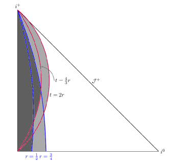
We now make a bootstrap assumption in order to use Proposition 6.3 to obtain the weak decay estimates. Recall the initial data involved a Schwarzschildean part being subtracted, see (1.8). Similarly we must subtract off the Schwarzschildean part from the perturbation. As in [14], define
In the case of our zero mode reduction of Kaluza-Klein, we take whenever at least one of the components are in the compact directions.
Figure 1. Regions where is vanishing (dark grey), between 0 and 1 (light grey) and identically 1 (white). In particular, is identically 1 towards and vanishing when .
Since is a known quantity, we introduce some notation to separate between the decay for terms involving and the decay for . Hence for we define
(6.5)
Recall also the weighted energy from (1.13) for the solution
(6.6)
As discussed after Theorem 1.2, we make the following bootstrap assumption. Define the time to be the maximal time such that the following inequality holds
(6.7)
for a fixed number such that and with being a local-in-time solution to (4.1) satisfying the wave-coordinate condition
(6.8)
Using the weighted Klainerman-Sobolev inequality and the bootstrap assumption one can now derive the following ‘weak decay’ estimates.
Assume (6.7) holds and is defined as in (6.5), then for and we have
(6.11)
(6.14)
where if and if .
Furthermore if then
(6.17)
Proof.
The proof of (6.14) follows from the weighted Klainerman-Sobolev estimate of Proposition 6.3 and the energy assumption (6.7). We obtain (6.11) for by integrating (6.14) from the hypersurface along lines with and fixed. One also needs the initial condition from the assumptions of our main Theorem 1.2, namely (1.10) implies
The final estimates for come from recalling that for any function
∎
These weak decay estimates immediately give the following decay on the inhomogeneities.
Assume (6.7) and (6.8) hold and let be as given in (4.1b). Then
Proof.
This follows from Proposition 5.7 and the weak decay estimates of Corollary 6.6.
∎
We end this section with a stand-alone Lemma which involves estimating the second-order derivatives landing on the Schwarzschildean part . Since the form of has been chosen in (6.4), this result comes from commuting through copies of and applying the results from Corollary 6.6.
In this section we will prove improved decay estimates for , valid only for a smaller number of vector fields, namely for . We first obtain estimates for and given in Proposition 7.3, followed by estimates of for in Proposition 7.5.
In the original paper by Lindblad and Rodnianski, it was shown that all but one component of obeys a decay rate. The ‘worst’ component has the slower decay rate. This was the decay rate originally suspected for all the components. Our choice of additional non-linearity, as discussed in Remark 5.8, has meant that the new variables pick up the better of these two decay rates.
We now turn to estimates of the best components of for , given in Proposition 7.5. These ‘best’ components have much better decay rates than the full set given before in Proposition 7.3. Note however that since we are using control obtained from the wave-coordinate condition condition, we only obtain estimates on and not . Thus Lemma 7.4 and Proposition 7.5 are completely unchanged from [14].
Let be a local-in-time solution of (4.1) such that (6.7) and (6.8) hold. Then
We now continue to the crux of this section, and derive ‘stronger’ estimates of all components of for the restricted range . The proof relies on using Corollary 6.1 again, this time with a non-trivial weight . Recall that in Corollary 6.1 there was a spacetime integral of where is the particular inhomogeneity being considered.
The inhomogeneity we consider comes from commuting through the PDE (4.1). This leads to the system
(7.1)
As in Lindblad and Rodnianski, we have introduced the shifted vector field where is a constant defined by . In particular, except when in which case . The commutator-like term is defined by
The estimates of and can be found in Proposition B.4. On the right hand side of (7.1) are the terms and which are estimated in the following lemma.
Let be a local-in-time solution of (4.1) such that (6.7) and (6.8) hold. Let and be as given in (4.1b). Then for we have
where it is understood that the term with vanishes if .
Proof.
The result follows from Proposition 5.7, Corollary 6.6 and the first estimate in Proposition 7.3.
∎
Proposition 7.7(Modified Proposition 10.2 from [14]).
Let be a solution of the generalised PDE (4.1).
Assume (6.7) holds, is defined as in (6.5) and and are defined as in (4.1b).
Let and be fixed. Then there exist constants and depending on and such that for all
where if or if .
Proof.
The proof follows by induction, as in [14]. The base case follows in a simpler but similar way to the main case. One assumes the step for and then considers the case of .
From (7.1) the following holds
From here we use Proposition 5.7 and Lemma 7.6 to estimate and . Lemma 6.8 gives an estimate for . Lastly Proposition B.4 gives an estimate on and .
One then collects together terms according to whether or . When we require strong estimates on the terms with a low number of ’s acting on , ie, of the form
Since there are no terms appearing here, we may use Proposition 7.5 which gives the necessary decay.
When one must use the induction hypothesis.
Putting this altogether gives an estimate on . Corollary 6.6 implies an estimate on .
Then inserting all this in Corollary 6.1 yields an integral inequality and the result then follows by Gronwall’s inequality.
∎
8. Energy Estimates
In this final section we will obtain an integrated energy inequality for using the following Proposition from [14]. Using this we will be able to apply a Gronwall type argument to deduce the improved inequality (1.16) for the energy.
Using Young’s inequality and the above Proposition 8.1 on the PDE (7.1) yields
(8.3)
The terms not ‘roughly’ in the form of the energy , defined in (6.6), are
(8.4)
and so these are estimated in the following Lemmas 8.3 to 8.5. First we state the main Theorem 8.2 proving (1.16) as the assumptions will be the same for Lemmas 8.3 to 8.5, but leave the proof until after the Lemmas.
Let be a local in time solution to (4.1) satisfying the wave gauge condition (5.1) on some maximal interval . Suppose for fixed and that for all and all we have
(8.5a)
(8.5d)
(8.5e)
For any constant satisfying there exist constants and , independent of , such that for sufficiently small the following holds for all
(8.6)
We begin by estimating the first pair of terms of (8.4) in Lemmas 8.3 and 8.4.
The proof follows as in [14] by using the decay estimates for and given in (8.5d). The stronger estimates required on and , are unchanged and given in (8.5a). For the full technical details we refer to [14].
∎
For the last term in (8.4), recall that , and thus , is determined by calculating directly from the definition in (6.4). Thus the next Lemma follows identically from [14], with the proof using Lemma 6.8 and Corollary B.1 on the term.
This means, up to some constant, we can use the background Minkowski volume form but still control an energy with volume form actually coming from the perturbed metric.
Then precisely as in [14], Lemmas 8.4, 8.6, 8.5 and the integrated energy inequality (8.3) imply
(8.7)
Similar to [14], define a quantity for the ‘good’ derivative
Note that apart from the derivative, this involves a spacetime integral compared to (6.6) which only has a spatial integral. Then for we obtain the inequality
One can now follow the argument in [14] and use Gronwall’s inequality and induction to deduce
for all . Since the constants are independent of time we have
for all .
∎
Remark 8.7.
As in Remark 6.4, the Kaluza-Klein example will have all variables independent of the torus coordinates. Thus any integrals in the above proof of Theorem 8.2 will pick up an additional, non-zero, constant from the volume of the torus.
Let be smooth initial data for (4.1), asymptotically flat in the sense of (1.10), with diffeomorphic to . Then there exists a constant such that for all and initial data such that
the solution to the system (4.1) can be extended to a global-in-time smooth solution in which the energy satisfies
(8.8)
where and depend only on .
Proof.
It holds that
Hence there exists a maximal on which the following bootstrap assumption holds
(8.9)
for some fixed with .
Condition (8.9) then allows us to use Propositions 7.3 and 7.5 to derive (8.5a) and Proposition 7.7 to derive (8.5d).
Theorem 8.2 then implies that we may choose a sufficiently small such that
Thus we have contracted the maximality of and so must be a global-in-time solution.
∎
Appendix A Non-Minimally Coupled Einstein-Maxwell-Scalar system from the mode reduction
In this section we derive the non-minimally coupled Einstein-Maxwell-Scalar system which arises from higher-dimensional vacuum gravity truncated to the zero mode over a . The dimensional coordinates are labelled by Greek indices and the dimensional flat spacetime labelled by Roman letters . The compact spacetime is labelled by , though note that are also frequently used in the literature.
By considering only the modes, the higher-dimensional metric depends only on the non-compact coordinates
(A.1)
It is standard to use an Ansatz to parametrise the space of solutions satisfying (A.1) in terms of the dimensional metric , collection of vector potentials and dilatons
(A.2)
where and .
The inverse is now
The higher-dimensional wave gauge (1.2) is equivalent to
(A.3a) is the standard wave-coordinate condition on the dimensional non-compact spacetime and (A.3b) reduces to the standard Lorenz gauge using an equivalent form of (A.3a), namely .
To determine the equations of motion, we express the Lagrangian for the Einstein equations in terms of the Ansatz (A.2).
where .
Recall the Einstein-Hilbert action is
Varying with respect to and respectively we obtain the following equations of motion:
(A.4a)
(A.4b)
(A.4c)
These equations will imply constraint equations for the initial data that must be satisfied on the initial surface . Note here is a 3-dimensional manifold and so the solution we seek will be such that is the pull-back of to , is the second fundamental form of and the restriction of and to is and respectively.
If is the normal to normalised such that , then the constraint equations are
(A.5)
where is the covariant derivative associated with .
Thus from the lower-dimensional perspective the constraint equations (A.5) can be interpreted as having some initial energy density coming from the scalar fields and Maxwell field strengths.
Theorem (2.1) implies that as . Thus as and so the radii of the stabilise to their initial (unperturbed) value. Similarly by inverting the Ansatz (A.2) one obtains that the vector potential as .
Acknowledgements
The author greatly thanks Pieter Blue for helpful discussions and advice during this project.
Appendix B Hardy Inequality and Further Identities
In this section we state some important results proved in [14], omitting the Lemmas which lead to these.
We next briefly state some key results from [14], the first two making use of the null frame. Recall the definition of the reduced wave operator where is the full (perturbed) metric. The final Proposition B.4 gives control on the commutator .
We introduce the shifted vector field where is a constant defined by . In particular, except when in which case . Note this definition implies the commutation property and thus .
[1]
Yvonne Choquet-Bruhat.
Un théorème d’instabilité pour certaines équations
hyperboliques non linéaires.
C. R. Acad. Sci. Paris Sér. A-B, 276:A281–A284, 1973.
[2]
Yvonne Choquet-Bruhat, Piotr T. Chrusciel, and Julien Loizelet.
Global solutions of the Einstein-Maxwell equations in higher
dimensions.
Class. Quant. Grav., 23:7383–7394, 2006.
[3]
Yvonne Choquet-Bruhat and Robert Geroch.
Global aspects of the cauchy problem in general relativity.
Comm. Math. Phys., 14(4):329–335, 1969.
[4]
D. Christodoulou and S. Klainerman.
The Global Nonlinear Stability of the Minkowski Space,
volume 41 of Princeton Mathematical Series.
Princeton University Press, Princeton, NJ, 1993.
[5]
Demetrios Christodoulou.
Global solutions of nonlinear hyperbolic equations for small initial
data.
Communications on Pure and Applied Mathematics, 39(2):267–282,
1986.
[6]
Y. Fourés-Bruhat.
Théorème d’existence pour certains systèmes d’équations aux
dérivées partielles non linéaires.
Acta Math., 88:141–225, 1952.
[7]
Theodor Kaluza.
Zum unitätsproblem in der physik.
Sitzungsberichte Preussische Akademie der Wissenschaften, pages
966–972, 1921.
[8]
S. Klainerman.
The null condition and global existence to nonlinear wave equations.
In Nonlinear systems of partial differential equations in
applied mathematics, Part 1 (Santa Fe, N.M., 1984), volume 23 of
Lectures in Appl. Math., pages 293–326. Amer. Math. Soc., Providence,
RI, 1986.
[9]
Sergiu Klainerman, editor.
Long time behavior of solutions to nonlinear wave equations,
Warsaw, 8 1983. International Congress of Mathematicians.
[10]
Oskar” Klein.
Quantentheorie und fünfdimensionale relativitätstheorie.
Zeitschrift für Physik, 37(12):895–906, 1926.
[11]
Philippe G. LeFloch and Yue Ma.
The global nonlinear stability of minkowski space for the einstein
equations in the presence of a massive field.
Comptes Rendus Mathematique, 354(9):948 – 953, 2016.
[12]
Hans Lindblad and Igor Rodnianski.
The weak null condition for Einstein’s equations.
C.R. Acad. Sci., 336:901–906, 2003.
[13]
Hans Lindblad and Igor Rodnianski.
Global existence for the einstein vacuum equations in wave
coordinates.
Communications in Mathematical Physics, 256(1):43–110, 2005.
[14]
Hans Lindblad and Igor Rodnianski.
The global stability of Minkowski space-time in harmonic gauge.
Ann. Math. (2), 171(3):1401–1477, 2010.
[15]
Julien Loizelet.
Solutions globales des équations d’Einstein-Maxwell.
Ann. Fac. Sci. Toulouse Math. (6), 18(3):565–610, 2009.
[17]
Jared Speck.
The global stability of the Minkowski spacetime solution to the
Einstein-nonlinear system in wave coordinates.
Analysis & PDE, 7(4):771–901, 2014.
[18]
Edward Witten.
Instability of the Kaluza-Klein Vacuum.
Nucl. Phys., B195:481–492, 1982.