HiNet: Hierarchical Classification with Neural Network

Abstract

Traditionally, classifying large hierarchical labels with more than 10000 distinct traces can only be achieved with flatten labels. Although flatten labels is feasible, it misses the hierarchical information in the labels. Hierarchical models like HSVM by Vural & Dy (2004) becomes impossible to train because of the sheer number of SVMs in the whole architecture. We developed a hierarchical architecture based on neural networks that is simple to train. Also, we derived an inference algorithm that can efficiently infer the MAP (maximum a posteriori) trace guaranteed by our theorems. Furthermore, the complexity of the model is only $O(n^{2})$ compared to $O(n^{h})$ in a flatten model, where $h$ is the height of the hierarchy.

1 Introduction

Large hierarchical classification with more than 10000 categories is a challenging task (Partalas et al. (2015)). Traditionally, hierarchical classification can be done by training a classifier on the flattened labels (Babbar et al. (2013)) or by training a classifier at each hierarchical node (Silla Jr & Freitas (2011)), whereby each hierarchical node is a decision maker of which subsequent node to route to. However, the second method scales inefficiently with the number of categories ($>10000$ categories). Models such as hierarchical-SVM (Vural & Dy (2004)) becomes difficult to train when there are 10000 SVMs in the entire hierarchy. Therefore for large number of categories, the hierarchy tree is flattened to produce single labels. While training becomes easier, the data then loses prior information about the labels and their structural relationships.

In this paper, we model the large hierarchical labels with layers of neurons directly. Unlike the traditional structural modeling with classifier at each node, here we represent each label in the hierarchy simply as a neuron.

2 Model

HiNet has different procedures for training and inference. During training, as illustrated in Figure 2, the model is forced to learn MAP (Maximum a Posteriori) hypothesis over predictions at different hierarchical levels independently. Since the hierarchical layers contain shared information as child node is conditioned on the parent node, we employ a combined cost function over errors across different levels. A combined cost allows travelling of information across levels which is equivalent to transfer learning between levels.

During inference, after predicting the posterior distribution at each level of the hierarchy, we employ a greedy downpour algorithm to efficiently infer the MAP (Maximum a Posteriori) hierarchical trace (Figure 4) from the posterior predictions at each level (Figure 2).

2.1 Hierarchy as Layers of Neurons

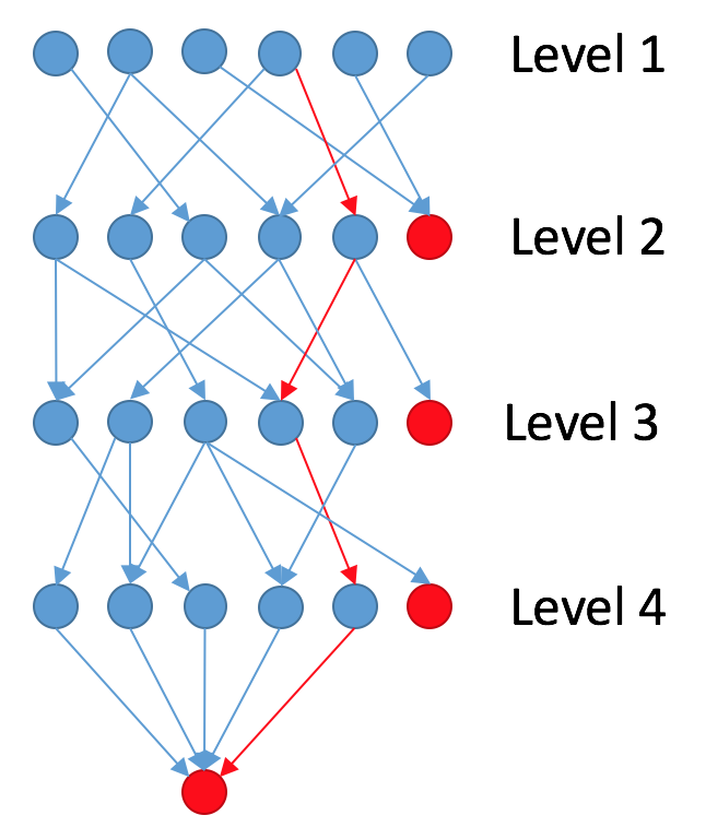
(a) DAG

(b) Tree

Figure 1: Neural network for modeling hierarchical relationships. Figure 1(a) shows a DAG (Directed Acyclic Graph) where a child neuron is possible to have more than one parents versus Figure 1(b) showing a tree where each child neuron only belongs to one parent. The path will end in a stop neuron (red neuron).

Using layers of neurons to model hierarchy is very efficient and flexible. It can be easily used to model a Directed Acyclic Graph (DAG) (Figure 1(a)) or a Tree (Figure 1(b)) by masking out the unnecessary connections. Unlike node-based architecture (Silla Jr & Freitas (2011); Vens et al. (2008); Dumais & Chen (2000)), whereby each node is an object with pointers to its child and parent, and takes up large memory, neural network models the connections as compact matrix which takes up much less memory. In order to model hierarchies of different length, we append a stop neuron (red neuron in Figure 1) at each layer. So a top-down path will end when it reaches the stop neuron.

2.2 Training

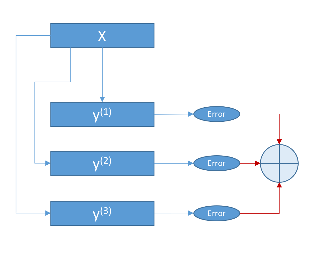
Figure 2: The above figure illustrates the architecture during training.

Figure 2 shows the model for transfer learning with combined cost function. Given an input feature $\mathbf{X}$ with multiple levels of outputs $\{\mathbf{y}^{(1)},\mathbf{y}^{(2)},\dots,\mathbf{y}^{(n)}\}$, where the outputs may have inter-level dependencies $p(\mathbf{y}^{(k)}|\mathbf{y}^{(1:k-1)},\mathbf{y}^{(k+1:n)})$. For each output level from network $f_{\theta_{k}}(\mathbf{X})=\mathbf{y}^{(k)}$ and its corresponding label $\tilde{\mathbf{y}}^{(k)}$. The combined cost is defined as $E=\sum_{k}^{n}\Big{(}\tilde{\mathbf{y}}^{(k)}-f_{\theta_{k}}(\mathbf{X})\Big{)}^{2}$ allows the parameters $\theta_{k}$ from different levels to exchange knowledge.

2.3 Inference

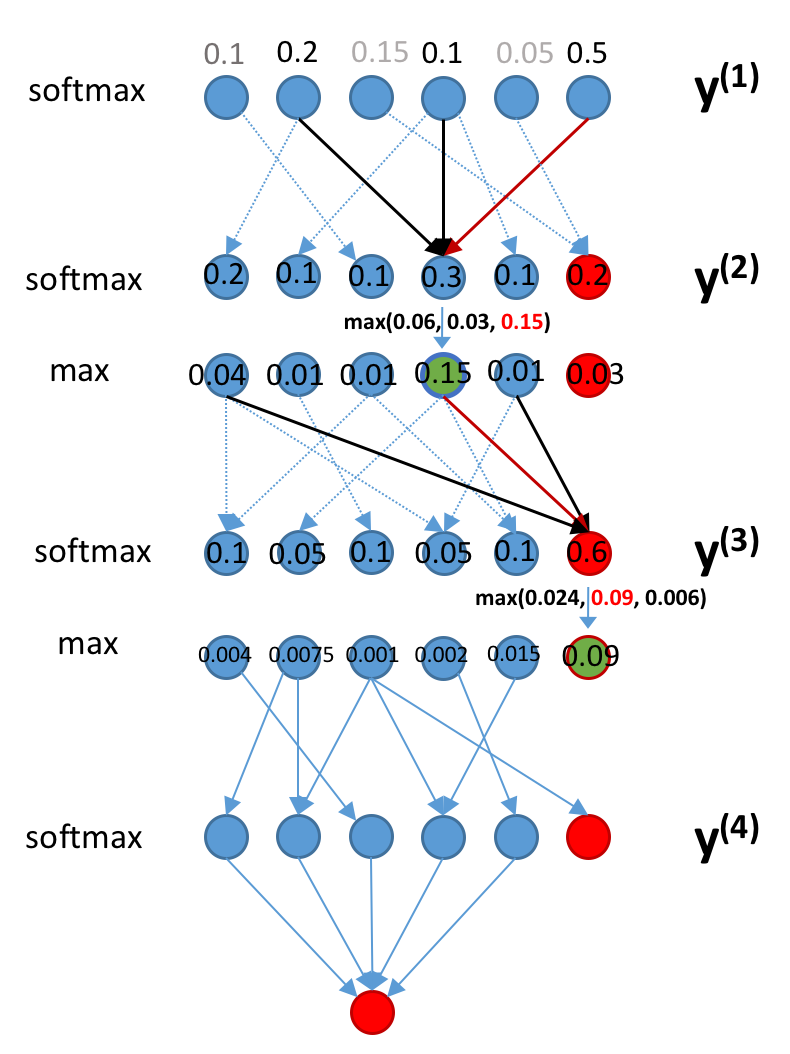
Figure 3: Inference: Downpour Algorithm

Figure 4: The above figure illustrates the downpour algorithm (Algorithm 1) for deriving the MAP trace.

Downpour Algorithm

Given output posteriors $\mathbf{y}^{(l)}=\{y_{a}^{(l)}\}$ at each layer $l\in\{1,\dots,K\}$

Define $T^{(l)}_{i}=[\mbox{ }]$ as MAP trace of neuron $i$ at level $l$

$T^{(1)}_{i}=[i]$

for layer $l=2$ to $k$ do

      

      Find MAP parent $A=\arg\max_{a}y_{b}^{(l)}y_{a}^{(l-1)}$

      $T_{b}^{(l)}=T_{A}^{(l-1)}.append(b)$

      Update $y_{b}^{(l)}$ = $\max_{a}y_{b}^{(l)}y_{a}^{(l-1)}$

end for

Find MAP level for stop neuron $s$

$L=\arg\max_{l}y_{s}^{(l)}$

return $T_{s}^{(L)}$

 

Algorithm 1 Downpour algorithm for inferencing the MAP trace.

During inference, as illustrated in Figure 4, the model will output a normalized probability distribution at each level $\{\mathbf{y}^{(1)},\mathbf{y}^{(2)},\dots,\mathbf{y}^{(k)}\}$, where $\mathbf{y}^{(k)}=\{y_{a_{k}}^{(k)}\}$ is a vector with indexes $a_{k}\in\{1,\dots,n\}$, where $n$ is the size of layer $k$, and $\sum_{a_{k}}y_{a_{k}}^{(k)}=1$. From the second level onwards, we include a stop neuron (red neuron) which is used for stopping the hierarchical trace. The path of the trace from top down ends in a stop neuron (red neuron). Define the MAP trace up to level $k$ which ends at stop neuron $s$ as $T^{(k)}_{a_{k}=s}=\arg\max\limits_{a_{1:k-1}}p(a_{1},a_{2},\dots,a_{k-1},a_{k}=s)$. The objective of the downpour in finding the MAP from the hierarchy is equivalent to finding the maximum MAP trace out of all MAP traces that ends in a stop neuron from different levels which is $T^{(L)}_{a_{L}=s}$ where $L=\arg\max_{k}T^{(k)}_{a_{k}=s}$. The probability of MAP trace at level $k$ can be derived greedily from the MAP trace at level $k-1$ as

$$p(T_{a_{k}}^{(k)})=\max_{a_{k-1}}p(a_{k}|a_{k-1})p(T_{a_{k-1}}^{(k-1)})$$ (1)

From Equation 1, we can derive Theorems 2.1-2.3 which prove that Downpour Algorithm will always yield the MAP trace of $T^{(L)}_{a_{L}=s}=\max_{n}p(T_{a_{n}=s}^{(n)})\geq p(a_{1},a_{2},\dots,a_{m}=s)$ $\forall m$.

Theorem 2.1.

For a greedy downpour that ends at a stop neuron at level $n$ with MAP trace $T_{a_{n}}^{(n)}$, then $p(S_{m})\leq p(T_{a_{n}}^{(n)})$ for every sequence $S_{m}=\{a_{1},a_{2},\dots,a_{n},\dots,a_{m}\}$ of $m\geq n$ that pass through $a_{n}$ or ends at $a_{n}$. Refer to Appendix A for proof.

Theorem 2.2.

For a MAP trace $T_{a_{n}=s}^{(n)}$ that ends at stop neuron $s$ at level $n$ such that $p(T_{a_{n}=s}^{(n)})\geq p(T_{a_{n}}^{(n)})$ $\forall a_{n}\neq s$, then $p(S_{m})\leq p(T_{a_{n}=s}^{(n)})$ for every sequence $S_{m}=\{a_{1},a_{2},\dots,a_{m}\}$ of $m>n$. Refer to Appendix A for proof.

Theorem 2.3.

The maximum of the MAP traces that end in a stop neuron from each level is $T_{a_{k}=s}^{(L)}$ where $L=\arg\max_{k}p(T_{a_{k}=s}^{(k)})$ is the MAP for the hierarchy, which means $p(T_{a_{k}=s}^{(L)})\geq p(S_{m})$ $\forall m$. Refer to Appendix A for proof.

3 Results and Conclusion

	DMOZ (Tree)	No. of Params
Flatten Network	39.2	$O(kn^{h})$
HiNet	41.4	$O(kn+hn^{2})$

Table 1: Accuracy on the DMOZ dataset (Partalas et al. (2015)) with 11947 classes. $k$: dimension of the first feature layer connected to the first hierarchical layer. $n$: dimension of each hierarchical layer. $h$: height of the hierarchy. For a fully dense hierarchy, the total number of classes is $n^{h}$.

We compared HiNet with a Flatten Network which have the same architecture except the output layer for HiNet is hierarchical as illustrated in Figure 2 and flatten for Flatten Network. The number of outputs for Flatten Network corresponds to the number of classes in the dataset. From the results, HiNet out-performs Flatten Network for both a Tree hierarchical dataset with much lesser parameters. We see that the number of parameters in the classification layer for Flatten Network is exponential to the maximum length of the trace. Thus for very deep hierarchies, the number of parameters in Flatten Network will be exponentially large while HiNet is always polynomial. This makes HiNet not only better architecture in terms of accuracy but also way more efficient in parameters space.

4 Appendix A

Proof for Theorem 2.1

For a greedy downpour that ends at a stop neuron at level $n$ with MAP trace $T_{a_{n}}^{(n)}$, then $p(S_{m})\leq p(T_{a_{n}}^{(n)})$ for every sequence $S_{m}=\{a_{1},a_{2},\dots,a_{n},\dots,a_{m}\}$ of $m\geq n$ that pass through $a_{n}$ or ends at $a_{n}$.

Proof.

for $m=n$, that is $p(T_{a_{n}}^{(n)})\geq p(S_{n})$. By definition $T_{a_{1}}^{(1)}=a_{1}$

$$\begin{split}p(T_{a_{n}}^{(n)})&=\max_{a_{n-1}}p(a_{n}|a_{n-1})p(T_{a_{n-1}}^{(n-1)})\\ &=\max_{a_{n-1}}p(a_{n}|a_{n-1})\max_{a_{n-2}}p(a_{n-1}|a_{n-2})p(T_{a_{n-2}}^{(n-2)})\\ &=\max_{a_{1:n-1}}p(a_{n}|a_{n-1})p(a_{n-1}|a_{n-2})\dots p(a_{1})\\ &=\max_{a_{1:n-1}}p(a_{n},a_{n-1},\dots,a_{1})\\ &\geq p(a_{n},a_{n-1},\dots,a_{1})\end{split}$$ (2)

for $m>n$, we just need to prove that $p(S_{m})\leq p(S_{n})$

$$\begin{split}p(S_{m})&=p(S_{n})p(a_{n+1},a_{n+2},\dots,a_{m}|S_{n})\\ &\geq p(S_{n})\end{split}$$ (3)

since $p(a_{n+1},a_{n+2},\dots,a_{m}|S_{n})\leq 1$ ∎

Proof for Theorem 2.2

For a MAP trace $T_{a_{n}=s}^{(n)}$ that ends at stop neuron $s$ at level $n$ such that $p(T_{a_{n}=s}^{(n)})\geq p(T_{a_{n}}^{(n)})$ $\forall a_{n}\neq s$, then $p(S_{m})\leq p(T_{a_{n}=s}^{(n)})$ for every sequence $S_{m}=\{a_{1},a_{2},\dots,a_{m}\}$ of $m>n$.

Proof.

from Theorem 2.1, $p(S_{m})\leq p(T_{a_{n}}^{(n)})\leq p(T_{a_{n}=s}^{(n)})$. ∎

Proof for Theorem 2.3

The maximum of the MAP traces that end in a stop neuron from each level is $T_{a_{k}=s}^{(L)}$ where $L=\arg\max_{k}p(T_{a_{k}=s}^{(k)})$ is the MAP for the hierarchy, which means $p(T_{a_{k}=s}^{(L)})\geq p(S_{m})$ $\forall m$.

Proof.

From Theorem 2.2, we have $p(T_{a_{n}=s}^{(n)})\geq p(S_{m})$ for every $m>n$, and from Theorem 2.1, we have $p(T_{a_{n}=s}^{(n)})\geq p(a_{1},a_{2},\dots,a_{n}=s)$. Therefore $\max_{n}p(T_{a_{n}=s}^{(n)})\geq p(a_{1},a_{2},\dots,a_{m}=s)$ $\forall m$. ∎

References

• Babbar etΒ al. (2013) Rohit Babbar, Ioannis Partalas, Eric Gaussier, and Massih-Reza Amini. On flat versus hierarchical classification in large-scale taxonomies. In Advances in Neural Information Processing Systems, pp.Β 1824–1832, 2013.
• Dumais & Chen (2000) Susan Dumais and Hao Chen. Hierarchical classification of web content. In Proceedings of the 23rd annual international ACM SIGIR conference on Research and development in information retrieval, pp.Β 256–263. ACM, 2000.
• Partalas etΒ al. (2015) Ioannis Partalas, Aris Kosmopoulos, Nicolas Baskiotis, Thierry Artieres, George Paliouras, Eric Gaussier, Ion Androutsopoulos, Massih-Reza Amini, and Patrick Galinari. Lshtc: A benchmark for large-scale text classification. arXiv preprint arXiv:1503.08581, 2015.
• SillaΒ Jr & Freitas (2011) CarlosΒ N SillaΒ Jr and AlexΒ A Freitas. A survey of hierarchical classification across different application domains. Data Mining and Knowledge Discovery, 22(1-2):31–72, 2011.
• Vens etΒ al. (2008) Celine Vens, Jan Struyf, Leander Schietgat, SaΕ‘o DΕΎeroski, and Hendrik Blockeel. Decision trees for hierarchical multi-label classification. Machine Learning, 73(2):185, 2008.
• Vural & Dy (2004) Volkan Vural and JenniferΒ G Dy. A hierarchical method for multi-class support vector machines. In ICML, pp.Β  105. ACM, 2004.