Consistent forcing scheme in the cascaded lattice Boltzmann method

Abstract

In this paper, we give a more pellucid derivation for the cascaded lattice Boltzmann method (CLBM) based on a general multiple-relaxation-time (MRT) frame through defining a shift matrix. When the shift matrix is a unit matrix, the CLBM degrades into an MRT LBM. Based on this, a consistent forcing scheme is developed for the CLBM. The applicability of the non-slip rule, the second-order convergence rate in space and the property of isotropy for the consistent forcing scheme is demonstrated through the simulation of several canonical problems. Several other existing force schemes previously used in the CLBM are also examined. The study clarifies the relation between MRT LBM and CLBM under a general framework.

PACS numbers

47.11.-j, 05.20.Dd

I Introduction

The lattice Boltzmann method (LBM), based on the simplified kinetic models, has gained remarkable success for the simulation of complex fluid flows and beyond, with applications (but not limited to) to micro flows, flows in porous media, turbulence, and multiphase flows Qian et al. (1995); Chen and Doolen (1998); Succi (2001); Shan and Chen (1993); Guo and Shu (2013); Gong et al. (2016). The LBM solves a specific discrete Boltzmann equation for the distribution functions, designed to recover the Navier-Stokes (N-S) equations in the macroscopic limit. The meso-scale nature of LBM allows its natural incorporation of micro and meso-scale physics, while the highly efficient algorithm makes it afforadable computationally Li et al. (2016a).

In the standard “collision-streaming” LBM algorithm, the simplest collision operator is the Bhatnagar-Gross-Krook (BGK) or single-relaxation-time (SRT) operator, which relaxes all the distribution functions to their local equilibrium counterparts at a common rate and the relaxation rate is related to the kinematic viscosity Qian et al. (1992). The multiple-relaxation-time (MRT) operator is another extensively used operater d’Humieres (1994), in which the collision is executed in the moment space and the relaxation rates for different moments can be different. More recently, a central-moments-based or cascaded operator was proposed by Geier et al. Geier et al. (2006). In the cascaded lattice Boltzmann method (CLBM), the collision is carried out in the space of central moment rather than that of raw moment as in the MRT LBM. Compared with the BGK operator, the MRT and cascaded operators can increase the numerical stability significantly Geier et al. (2006); Lallemand and Luo (2000); Lycett-Brown and Luo (2016); Fei and Luo (2016). Athough the collision steps in these LBMs are quite different, the streaming steps are carried out in the same way by streaming the post-collision distributions to their neighbors. It should be noted that other collision operaters, like the two-relaxation-time (TRT) operator Ginzburg (2005); Ginzburg et al. (2008) and the entropic operator Ansumali et al. (2003); Ansumali and Karlin (2000) are also very popular in the lattice Boltzmann community.

In many fluid systems, an external or internal force field plays an important role in the flow behaviours. To incorporate the force effect, different force treatments have been proposed in the literature Shan and Chen (1993); He et al. (1999); Buick and Greated (2000); Ladd and Verberg (2001). In 2002, Guo et al analyzed the discrete lattice effects on the forcing scheme and developed a representation of the forcing term Guo et al. (2002). Guo et al. then extended the method to the MRT LBM in 2008 Guo and Zheng (2008). Up to now, the method by Guo et al has been widely used in the LBM simulation. For the CLBM simulation, there is still no commonly used forcing scheme, while one scheme by method of central moments has been proposed by Premnath et al .Premnath and Banerjee (2009). In Ref. Lycett-Brown and Luo (2014), Lycett-Brown and Luo incorporate the forcing scheme for the BGK LBM into the CLBM directly. As analysed by De Rosis De Rosis (2017a), the method proposed by Premnath et al may encounter cumbersome practical implementations. Based on the central moments of a discrete equilibrium, a forcing scheme has been developed in De Rosis (2017a).

However, there is still no analysis about whether these forcing schemes in the CLBM are consistent with the forcing scheme in the MRT LBM Guo and Zheng (2008) and the original scheme proposed by Guo et al in the BGK LBM Guo et al. (2002). In this paper, we propose a more pellucid derivation for the CLBM by defining a shift matrix. This definition clarifies the relationship between MRT LBM and CLBM. Based on this frame, we present a consistent forcing scheme in CLBM, and show that the privious methods in Refs. Premnath and Banerjee (2009); Lycett-Brown and Luo (2014); De Rosis (2017a) are not consistent. The rest of the paper is structured as follows: Section II gives the new derivation for the cascaded LBM and presents the consistent forcing scheme. Section III presents a short analysis for the privious forcing schemes. Numerical verifications are presented in Sec. IV. Finally, conclusions of this work are made in Sec. V.

II CASCADED LBM AND CONSISTENT FORCING SCHEME

II.1 Cascaded LBM

Without losing the generality, the D2Q9 lattice Qian et al. (1992) is adopted here. The lattice speed $c=\Delta{x}/\Delta{t}=1$ and the lattice sound speed $c_{s}=1/\sqrt{3}$ are adopted, in which $\Delta{x}$ and $\Delta{t}$ are the lattice spacing and time step. The discrete velocities ${{\bf{e}}_{i}}=\left[{\left|{{e_{ix}}}\right\rangle,\left\langle{{e_{iy}}}\right|}\right]$ are defined as

$$\begin{array}[]{l}\left|{{e_{ix}}}\right\rangle={[0,1,0,-1,0,1,-1,-1,1]^{\top}},\\ \left|{{e_{iy}}}\right\rangle={[0,0,1,0,-1,1,1,-1,-1]^{\top}}.\\ \end{array}$$ (1)

where $i=0...8$, ${\left|\cdot\right\rangle}$ denotes a nine-dimensional colunm vector, and the superscript $\top$ denotes the transposition.

Here we propose a new derivation for the CLBM, which is different from and more intelligible than that given by Geier et al Geier et al. (2006). We first define the raw and central velocity moments of the discrete distribution function (DF) ${{f_{i}}}$,

$$\begin{array}[]{l}{k_{{mn}}}=\left\langle{{f_{i}}\left|{e_{ix}^{m}e_{iy}^{n}}\right.}\right\rangle,\\ {{\tilde{k}}_{{mn}}}=\left\langle{{f_{i}}\left|{{{({e_{ix}}-{u_{x}})}^{m}}{{({e_{iy}}-{u_{y}})}^{n}}}\right.}\right\rangle,\\ \end{array}$$ (2)

where ${u_{x}}$ and ${u_{y}}$ are the horizontal and vertical velocity components. The equilibrium values $k_{{}_{{mn}}}^{eq}$ and $\tilde{k}_{{mn}}^{eq}$ are defined analogously by using the discrete equilibrium distribution function (EDF) ${f_{i}^{eq}}$ in Eq. (2). In the previous CLBM, the recombined raw moments are adopted,

$$\left|{{T_{i}}}\right\rangle=\left[{{k_{00}},{k_{10}},{k_{01}},{k_{20}}+{k_{02}},{k_{20}}-{k_{02}},{k_{11}},{k_{21}},{k_{12}},{k_{22}}}\right]^{\top},$$ (3)

so do the recombined central moments $\tilde{T}_{i}$. The transformantion from the discrete DF to its raw moments can be realized through a transformation matrix ${\bf{M}}$, and the shift from the raw moments to central moments can be realized though a shfit matrix ${\bf{N}}$,

$$\begin{array}[]{l}\left|{{T_{i}}}\right\rangle={\bf{M}}\left|{{f_{i}}}\right\rangle,\\ \left|{{{\tilde{T}}_{i}}}\right\rangle={\bf{N}}\left|{{T_{i}}}\right\rangle.\\ \end{array}$$ (4)

The explicit forms for ${\bf{M}}$ and ${\bf{N}}$ can be obtained through the defination in Eqs. (2,3,4). Explicitly, the transformation matrix ${\bf{M}}$ is expressed as Lycett-Brown and Luo (2014)

$${\bf{M}}=\left[\begin{array}[]{c c c c c c c c c}1&1&1&1&1&1&1&1&1\\ 0&1&0&-1&0&1&-1&-1&1\\ 0&0&1&0&-1&1&1&-1&-1\\ 0&1&1&1&1&2&2&2&2\\ 0&1&-1&1&-1&0&0&0&0\\ 0&0&0&0&0&1&-1&1&-1\\ 0&0&0&0&0&1&1&-1&-1\\ 0&0&0&0&0&1&-1&-1&1\\ 0&0&0&0&0&1&1&1&1\\ \end{array}\right],$$ (5)

and the shift matrix ${\bf{N}}$ is given by

$${\bf{N}}=\left[\begin{array}[]{c c c c c c c c c}1&0&0&0&0&0&0&0&0\\ -{u_{x}}&1&0&0&0&0&0&0&0\\ -{u_{y}}&0&1&0&0&0&0&0&0\\ u_{x}^{2}+u_{y}^{2}&-2{u_{x}}&-2{u_{y}}&1&0&0&0&0&0\\ u_{x}^{2}-u_{y}^{2}&-2{u_{x}}&2{u_{y}}&0&1&0&0&0&0\\ {u_{x}}{u_{y}}&-u_{y}&-u_{x}&0&0&1&0&0&0\\ -u_{x}^{2}{u_{y}}&2{u_{x}}{u_{y}}&u_{x}^{2}&-{u_{y}}/2\par&-{u_{y}}/2&-2u_{x}&1&0&0\\ -u_{y}^{2}{u_{x}}&{u_{y}}^{2}&2{u_{x}}{u_{y}}&-{u_{x}}/2\par&{u_{x}}/2&-2u_{y}&0&1&0\\ u_{x}^{2}u_{y}^{2}&-2{u_{x}}u_{y}^{2}&-2{u_{y}}u_{x}^{2}&u_{x}^{2}/2+u_{y}^{2}/2&u_{y}^{2}/2-u_{x}^{2}/2&4{u_{x}}{u_{y}}&-2{u_{y}}&-2{u_{x}}&1\\ \end{array}\right].$$ (6)

In the collision step for the cascaded LBM, the central moments ($\tilde{T}_{i}$) of the discrete DF ${{f_{i}}}$ are relaxed to their equilibrium values $\tilde{T}_{i}^{eq}$. Thus the post-collision central moments are

$$\left|{\tilde{T}_{i}^{*}}\right\rangle =({\bf{I-S}})\left|{{{\tilde{T}}_{i}}}\right\rangle+{\bf{S}}\left|{\tilde{T}_{i}^{eq}}\right\rangle$$ (7)

$$=({\bf{I-S}}){\bf{NM}}\left|{{f_{i}}}\right\rangle+{\bf{SNM}}\left|{f_{i}^{eq}}\right\rangle.$$

where ${\bf{S}}=diag({s_{0}},{s_{1}},{s_{1}},{s_{b}},{s_{2}},{s_{2}},{s_{3}},{s_{3}},{s_{4}})$ is a diagonal relaxation matrix. The kinematic and bulk viscosities are related to the relaxation parameters ${s_{2}}=1/(3\upsilon+0.5)$ and ${s_{b}}=1/(3\xi+0.5)$, respectively. As recommened in Refs. Geier et al. (2006); Premnath and Banerjee (2009); Lycett-Brown and Luo (2014), the equalibrium central moments of the discrete (EDF) ${f_{i}^{eq}}$ are set equal to the continuous central moments of the Maxwellian-Boltzmann distribution in continuous velocity space. To be specific,

$$\left|{\tilde{T}_{i}^{eq}}\right\rangle=\left[{\rho,0,0,2\rho c_{s}^{2},0,0,0,0,\rho c_{s}^{4}}\right]^{\top},$$ (8)

where $\rho$ is the fluid density, thus the matrix manipulation is not needed for $\left|{\tilde{T}_{i}^{eq}}\right\rangle$. The corresponding discrete EDF ${f_{i}^{eq}}$ is in fact a generalized local equilibrium Asinari (2008); Premnath and Banerjee (2009). Due to the definitions of the transformation and shift matrices, both of them are reversible (explicit expressions for ${\bf{M}}^{-1}$ and ${\bf{N}}^{-1}$ are given in the Appendix). The post-collision discrete DF is given by

$$\left|{f_{i}^{*}}\right\rangle={{\bf{M}}^{-1}}{{\bf{N}}^{-1}}\left|{\tilde{T}_{i}^{*}}\right\rangle.$$ (9)

In the streaming step, the post-collision discrete DF in space $\bf{x}$ and time $t$ streams to its neighbor in the next time step as usual Guo et al. (2002); Guo and Zheng (2008); Liu et al. (2016),

$${f_{i}}(\textbf{x}+{\textbf{e}_{i}}\Delta t,t+\Delta t)=f_{i}^{*}(\textbf{x},t).$$ (10)

Using the Chapman-Enskog analysis, the incompressible N-S equaltions can be reproduced in the low-Mach number limit Premnath and Banerjee (2009); Lycett-Brown and Luo (2014). The hydrodynamics variables are obtained as,

$$\rho=\sum\nolimits_{i}{{f_{i}}},~{}~{}~{}\rho\textbf{u}=\sum\nolimits_{i}{{f_{i}}}{\textbf{e}_{i}}.$$ (11)

It can be found that when the shift matrix ${\bf{N}}$ is a unit matrix, the CLBM degrades into a non-orthogonal MRT LBM Liu et al. (2016). Thus the present derivation is based on a general multiple-relaxation-time frame and clarifies the relationship between the MRT LBM and CLBM.

II.2 Consistent forcing scheme

Inspired by the method proposed by Guo et al Guo et al. (2002); Guo and Zheng (2008), to incoporate an external or internal force field ${\bf{F}}=[{F_{x}},{F_{y}}]$ into the CLBM , the collision step for central moments in Eq. (6) is modified by

$$\left|{\tilde{T}_{i}^{*}}\right\rangle =({\bf{I-S}})\left|{{{\tilde{T}}_{i}}}\right\rangle+{\bf{S}}\left|{\tilde{T}_{i}^{eq}}\right\rangle+({\bf{I-S}}/2)\left|{{C_{i}}}\right\rangle$$ (12)

$$={\bf{NM}}\left|{{f_{i}}}\right\rangle+{\bf{SNM}}\left|{f_{i}^{eq}}\right\rangle+({\bf{I-S}}/2){\bf{NM}}\left|{{R_{i}}}\right\rangle$$

where ${{R_{i}}}$ is the force effect term, which can be obtained by He et al. (1998),

$${{R_{i}}}=\frac{{\bf{F}}}{\rho}\cdot\frac{{\left({{\textbf{e}_{i}}-\textbf{u}}\right)}}{{c_{s}^{2}}}f_{i}^{eq}.$$ (13)

When using the generalized local equalibrium, the central moments for $\left|{{R_{i}}}\right\rangle$ can be computed as,

$$\left|{{C_{i}}}\right\rangle=[0,{F_{x}},{F_{y}},0,0,0,c_{s}^{2}{F_{x}},c_{s}^{2}{F_{y}},0]^{\top},$$ (14)

so the explicit formulation and matrix manipulation for $\left|{{R_{i}}}\right\rangle$ in Eq. (12) are not needed in the practical implement. Then the fluid velocity is defined by,

$$\rho{\bf{u}}=\sum\nolimits_{i}{{f_{i}}}{{\bf{e}}_{i}}+\frac{{\Delta t}}{2}{\bf{F}}.$$ (15)

Remark 1. In Eq. (12), the forcing effects in the present scheme are considered by means of central moments, which is compatible with the basic ideology (collision in the central moments space) in the CLBM.

Remark 2. When the shift matrix ${\bf{N}}$ in Eq. (12) is a unit matrix, the CLBM with the present forcing scheme will degrade into the MRT LBM proposed by Liu et al. Liu et al. (2016) with some high-order terms. It is known that the method of Liu et al. is equivalent to the method of Guo et al. in Guo and Zheng (2008).

Remark 3. In the orginal forcing scheme proposed by Guo et al. Guo et al. (2002), the forcing effect term is defined by ${R_{Gi}}={w_{i}}\left[{\left({{\textbf{e}_{i}}-\textbf{u}}\right)/c_{s}^{2}+\left({{\textbf{e}_{i}}\cdot\textbf{u}}\right){\textbf{e}_{i}}/c_{s}^{4}}\right]{\bf{F}}$. It is easy to find that the forcing effect term in Eq. (13) is equivalent to ${R_{Gi}}$ plus some high-order terms. The constraint conditions for the forcing effect term (see Eq. (7) in Guo et al. (2002)) are also satisfied in the present scheme. In particular, when all the parameters in the matrix ${\bf{S}}$ are set equal to ${s_{2}}$, the CLBM with the present forcing scheme will degrade into the BGK LBM with forcing scheme by Guo et al. in Guo et al. (2002) with a generalized local equilibrium.

Remark 4. It is also found (see in Sec. IV) that the zero-slip velocity boundary condition for the half-way bounce-back rule (${s_{3}}=(16-8{s_{2}})/(8-{s_{2}})$) discussed in Guo and Zheng (2008); Ginzburg and d’Humières (2003) is also applicable to the present forcing scheme.

From the above, we name the present forcing scheme as a consistent scheme in the CLBM.

III OTHER FORCING METHODS

In this section, several other methods to incorporate forcing effects into the CLBM in the literature are summerized. To show the inconsistencies in these methods, they are all written in the general multiple-relaxation-time frame proposed in Sec. II.1.

III.1 Forcing scheme by Premnath et al.

In 2009, Premnath et al. Premnath and Banerjee (2009) proposed a forcing scheme to incorporate forcing terms into CLBM. Inspired by He et al. He et al. (1998), they proposed a change of continuous distribution function $f$ due to the presence of a force field,

$$\Delta f=\frac{{\bf{F}}}{\rho}\cdot\frac{{\left({{e_{i}}-u}\right)}}{{c_{s}^{2}}}{f^{M}},$$ (16)

where ${f^{M}}$ is the Maxwellian-Boltzmann distribution in continuous velocity space. The central moments of $\Delta f$ is then incorporated into the collision stage in central moments by,

$$\left|{\tilde{T}_{i}^{*}}\right\rangle{\rm{}}=({\bf{I}}-{\bf{S}})\left|{{{\tilde{T}}_{i}}}\right\rangle+{\bf{S}}\left|{\tilde{T}_{i}^{eq}-{C_{Pi}}/2}\right\rangle.$$ (17)

The discrete counterpart of $\Delta f$ is also needed to obtain the post-collision discrete DF,

$$\left|{f_{i}^{*}}\right\rangle={{\bf{M}}^{-1}}{{\bf{N}}^{-1}}\left|{\tilde{T}_{i}^{*}}\right\rangle+\left|{\Delta{f_{i}}}\right\rangle$$ (18)

The fluid velocity is defined as in Eq. (15).

It should be noted that the original derivation in Premnath and Banerjee (2009) is tedious, and ${C_{Pi}}$ and ${\Delta{f_{i}}}$ are corresponding to ${{\hat{\sigma}}_{{x^{m}}{y^{n}}}}$ and ${S_{a}}$ in Premnath and Banerjee (2009), respectively. Though the method is compatible with the central-moment-based collision operator, the explicit formulations of ${\Delta{f_{i}}}$ and its raw moments are needed, which makes the practical implementations cumbersome De Rosis (2017a). Moreover, in their definition for the central moments of $\Delta f$, they removed the high-order nonzero terms arbitraily,

$$\left|{{C_{Pi}}}\right\rangle=[0,{F_{x}},{F_{y}},0,0,0,0,0,0]^{\top}.$$ (19)

Though they think that the high-order terms do not affect consistency, we certainly see some inconsistencies. For example, the first element in ${\Delta{f_{i}}}$ and ${R_{Gi}}$ are apparently inconsistent,

$$\begin{array}[]{l}\Delta{f_{0}}=-2{F_{x}}{u_{x}}-2{F_{y}}{u_{y}}+O({u^{3}}),\\ {R_{G0}}=-3{F_{x}}{u_{x}}-3{F_{y}}{u_{y}},\\ \end{array}$$ (20)

which will affect numerical performaces (see in Sec. IV).

III.2 Forcing scheme by Lycett-Brown and Luo

Cascaded LBM was first used to simulated multiphase flows by Lycett-Brown et al. Lycett-Brown and Luo (2014) in 2014. In their method, three forcing schemes, the Shan-Chen method Shan and Chen (1993), the EDM method Kupershtokh et al. (2009) and Guo method Guo et al. (2002) were adopted directly in the CLBM.

As discussed in the literature Huang et al. (2011); Li et al. (2012), both the Shan-Chen method and EDM method obtain some additional terms in the recovered macroscopic equations. These addtitional terms may have some positive effets on the numerial performance of the Shan-chen model Shan and Chen (1993), but it is not sensible to use the Shan-Chen method and EDM method in the CLBM directly for general flows. In the present work, we only consider the CLBM with the forcing scheme of Guo et al. Thus the collision stage in central moments can be written as,

$$\left|{\tilde{T}_{i}^{*}}\right\rangle=({\bf{I}}-{\bf{S}})\left|{{{\tilde{T}}_{i}}}\right\rangle+{\bf{S}}\left|{\tilde{T}_{i}^{eq}}\right\rangle+(1-{s_{2}}/2){\bf{NM}}\left|{{R_{Gi}}}\right\rangle,$$ (21)

while the fluid velocity is also defined as in Eq. (15).

III.3 Forcing scheme by De Rosis

Recently, De Rosis proposed an alternative method to incorporate forcing effects into the CLBM. The collision stage in central moments is,

$$\left|{\tilde{T}_{i}^{*}}\right\rangle=({\bf{I}}-{\bf{S}})\left|{{{\tilde{T}}_{i}}}\right\rangle+{\bf{S}}\left|{\tilde{T}_{i}^{eq}}\right\rangle+\frac{1}{2}\left|{{\xi_{i}}}\right\rangle,$$ (22)

where, ${\xi_{i}}$ is the central moment of the forcing effect term, and the fluid velocity is also defined as in Eq. (15).

Unfortunately, there is a typographical error in Eq. (16) of the paper De Rosis (2017a). Particularly, the sign in front of ${\xi_{i}}/2$ is not correct. In this method, the forcing term is defined by the truncated local equilibrium DF, which gives a lot of velocity terms in ${\xi_{i}}$ (see Eq. (15) in De Rosis (2017a)). Due to the definition of central moments, it is not recommended to include velocity terms in ${\xi_{i}}$. Thus there are some spurious effects in this method. It is also noted that the computational load for ${\xi_{i}}$ is much higher than that of ${C_{i}}$ in Eq. (14). Comparing Eq. (22) with Eq. (12), it is seen that the relaxation rate for each element of ${\xi_{i}}$ is 1.0 in this method, which is not consistent with the multiple-ralaxation-time ideology in the CLBM.

Remark 5. In the CLBM, the first three central moments are conserved moments, corresponding to conservations of mass and momentum. Thus the first two parameters (${s_{0}}$ and ${s_{1}}$) in the relaxation matrix ${\bf{S}}$ can be chosen freely. This property is retained in the present forcing scheme and the method by Premnath et al., because the relaxation matrix acts on the forcing effect terms in these two methods (see Eq. (12) and Eq. (17)). However, ${s_{1}}$ need to be set equal to ${s_{2}}$ in method by Lycett-Brown and Luo, and to be 1.0 method by De Rosis, to guarantee the conservation of momentum.

Remark 6. If ${s_{3}}$ is chosen to be 2.0, the forcing effect on the third-order central moment in Eq. (11) is removed. Thus the present scheme degrades into the forcing scheme by Premnath et al. only when ${s_{3}}=2.0$. Similarly, only when ${s_{3}}=1.0$, the difference between the forcing scheme by De Rosis and the present scheme can be removed. And in the BGK limitation, all the parameters are equal to ${s_{2}}$, at which the present scheme degrades into the method by Lycett-Brown and Luo.

Remark 7. In 2015, an improved forcing scheme for the pseudopotential model in multiphase flow was proposed by Lycett Brown and Luo Lycett-Brown and Luo (2015). The imporved forcing scheme was then incorporated into the CLBM for multiphase flow with large-density-ratio at high Reynolds and Weber numbers Lycett-Brown and Luo (2016). The basic philosophy of the improved forcing scheme is making artificial errors in the pressure tensor to counteract the lack of thermodynamical consistency in the original pseudopotential model. Thus it is not suitable for general flows with a force field. Besides, another simple forcing term was used in CLBM to simulate turbulent channel flow in 2011 Freitas et al. (2011). However, as analysed by Guo et al. Guo et al. (2002), the method used in Freitas et al. (2011) can not recover the accurate macroscopic equations with a spatial and temporal variational force field in the BGK LBM, not to mention in the CLBM.

IV NUMERICAL SIMULATIONS

In these section, we conduct several benchmark cases to verify the consistent forcing scheme. The other three methods mentioned in Sec. III are also used to validate our arguments. The three methods and present method are denoted by ${M_{1}}$, ${M_{2}}$, ${M_{3}}$ and ${M_{p}}$, respectively. In the simulation, ${s_{1}}$ is set to be ${s_{2}}$ in ${M_{2}}$, but to be 1.0 in other methods.

IV.1 Steady Poiseuille flow

The first problem considered is a steady Poiseuille flow driven by a constant body force F. The flow direction is set to be positive direction of the $x$ axial, thus ${\bf{F}}=[{F_{x}},0]$. The analytical solution for a channel of width $2L$ is,

$${{\bf{u}}_{a}}=\left[{\frac{{{F_{x}}}}{{2\nu}}(1-\frac{{{y^{2}}}}{{{L^{2}}}}),~{}0}\right].$$ (23)

The periodic boundary conditions are used in the flow direction, while the standard half-way bounce-back boundary scheme is used for non-slip boundary conditions at the walls. Due to the simple flow property, the length of the channel is set to $3\Delta x$ to save the computational load.

As analysed by previous researchers Ginzburg and d’Humières (2003); Guo and Zheng (2008), when the relaxation rate for the energy flux is chosen to be ${s_{3}}=(16-8{s_{2}})/(8-{s_{2}})$, no numerical slips occurs in the Poiseuille flows for the MRT LBM. To check its applicability in the CLBM with the present forcing scheme, we first choose kinematic viscity $\upsilon=0.5$, ${F_{x}}=0.01$, and only three nodes are used to cover the channel width ($2L=3\Delta x$) . We change ${s_{3}}$ from 0.2 to 1.8 with a 0.05 interval, and the other parameters are set equal to ${s_{2}}$. The residual error ${E_{R}}<{1\times 10^{-9}}$ is used as the convergent criterion, and the relative error ${E_{2}}$ is calculated for the following analysis,

$${E_{R}}=\sqrt{\frac{{\sum{{{({\mathbf{u}_{(t+1000\delta t)}}-{\mathbf{u}_{t}})}^{2}}}}}{{\sum{\mathbf{u}_{(t+1000\delta t)}^{2}}}}},~{}~{}{E_{2}}=\sqrt{\frac{{\sum{{{(\mathbf{u}-{\mathbf{u}_{a}})}^{2}}}}}{{\sum{{\mathbf{u}_{a}}^{2}}}}}.$$ (24)

For this case, the needed value for non-slip rule of ${s_{3}}$ is 1.6. As shown in Fig. 1, the relative error for each method changes with different values of ${s_{3}}$. But only in the present method, the minimum value of ${E_{2}}$ is achieved when ${s_{3}}=1.6$. And when the non-slip condition is satisfied, the relative error reaches a quite small value even in a very coarse mesh.

To further confirm the consistent non-slip boundary condition in the present method, we conduct several others cases. Now the channel width is set to be 50 nodes, and different body forces ${F_{x}}=[1\times{10^{-6}},3\times{10^{-6}},5\times{10^{-6}},7\times{10^{-6}}]$ are considered. The configurations are the same as those in Premnath and Banerjee (2009), ${s_{3}}$ is chosen according to the non-slip rule, while other relaxation parameters are 1.754. As shown in Table 1, the relative errors for $M_{1}$ are $O({10^{-4}})$, which is consistent with the results in Premnath and Banerjee (2009), where the non-slip rule was not considered. Compared with these three methods, the relative errors for the present method are much smaller with 5-6 orders, which confirms the availibility of the non-slip rule in the present method. For the differeces between the three methods in this case, it is easy to analyze that the error terms in the three methods are in a descending order of $M_{1}$, $M_{2}$, and $M_{3}$.

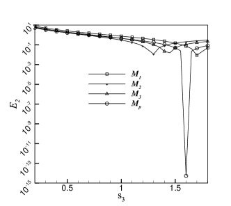
Figure 1: ${E_{2}}$ changes with ${s_{3}}$ for different methods.

Table 1: ${E_{2}}(\times{10^{4}})$ with different magnitudes of force for different methods.

${F_{x}}$	$M_{1}$	$M_{2}$	$M_{3}$	$M_{p}$
$1\times{10^{-6}}$	2.739	2.339	1.113	$1.044\times{10^{-6}}$
$3\times{10^{-6}}$	2.739	2.339	1.113	$3.173\times{10^{-6}}$
$5\times{10^{-6}}$	2.739	2.339	1.113	$5.527\times{10^{-6}}$
$7\times{10^{-6}}$	2.739	2.339	1.113	$7.296\times{10^{-6}}$

IV.2 Steady Taylor-Green flow

For the two-dimensional steady incompressible flow in a periodic box $N\times N$, if the force field is given by,

$${\bf{F}}(x,y)=2\nu{u_{0}}{\phi^{2}}\left[{\cos(\phi x)\cos(\phi y),\sin(\phi x)\sin(\phi y)}\right],$$ (25)

the flow has the following analytical solution,

$$\begin{array}[]{l}{\bf{u}}_{a}(x,y)={u_{0}}[\sin(\phi x)\sin(\phi y),\cos(\phi x)\cos(\phi y)],\\ p_{a}(x,y)={p_{0}}+0.25u_{0}^{2}[\cos(2\phi x)-\cos(2\phi y)],\end{array}$$ (26)

where $\phi=2\pi/N$, ${p_{0}}={\rho_{0}}c_{s}^{2}$ and ${\rho_{0}}=1$. The flow is known as steady Taylor-Green flow or four-rolls mill Taylor (1934), and is characterized by Reynolds number, ${\mathop{\rm Re}\nolimits}={u_{0}}\pi/v$.

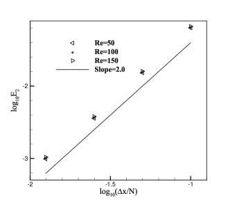
Figure 2: ${E_{2}}$ changes with grid size for the present scheme at ${\mathop{\rm Re}\nolimits}=50,100$ and $150$.

Table 2: ${E_{2}}(\times{10^{2}})$ and convergence rates (CR) for different forcing methods with different values of Reynolds number.

	${\mathop{\rm Re}\nolimits}=50$				${\mathop{\rm Re}\nolimits}=100$				${\mathop{\rm Re}\nolimits}=150$
$N/\Delta x$	$M_{P}$	$M_{1}$	${M_{2}}$	$M_{3}$	$M_{P}$	$M_{1}$	${M_{2}}$	$M_{3}$	$M_{P}$	$M_{1}$	${M_{2}}$	$M_{3}$
10	6.3752	6.5748	6.5522	6.3959	6.5448	6.6456	6.6398	6.5660	6.6482	6.7162	6.7135	6.6698
20	1.5275	1.6263	1.6051	1.5538	1.5788	1.6283	1.6227	1.6063	1.5974	1.6305	1.6279	1.6261
40	0.3587	0.3969	0.3782	0.3843	0.3719	0.3961	0.3909	0.4074	0.3796	0.3957	0.3933	0.4145
80	0.0986	0.1141	0.1037	0.1498	0.1025	0.1109	0.1076	0.1543	0.1040	0.1098	0.1082	0.1560
CR	2.0133	1.9579	2.0031	1.8264	2.0076	1.9753	1.9896	1.8213	2.0068	1.9848	1.9917	1.8222

In the simulation, the computational domain covered by a series of grid nodes, $N/\Delta x=\left[{10,20,40,80}\right]$, with three different conditions at ${\mathop{\rm Re}\nolimits}=[50,100,150]$. To weaken the artificial compressibility, ${u_{0}}=0.05$ is used in all the cases, ${s_{b}}$ is given equal to ${s_{2}}$, while the remaining relaxation parameters are set to unity. The relative error ${E_{2}}$ is computed from Eq. (24). The relationship between grid size and ${E_{2}}$ of the present forcing scheme at different Reynolds numbers is presented in Fig. 2. The slops at ${\mathop{\rm Re}\nolimits}=50,100$ and $150$ are 2.0133, 2.0076 and 2.0068, respectively. This demonstrates the scheme preposed has second-order accuracy in space. The relative error for each method is shown in Table 2. It is found that the present scheme achives the smallest relative error for every grid resolution at every Reynolds number. Due to the discrete equilibriun central moments used in $M_{3}$ (see Eq. (10) in De Rosis (2017b)), some additional errors are introduced into the CLBM, and this effect becomes evident when the mesh size is small. It is the reason why this method manifests an outlier for the finest grid resolution. Generally, each method presents a second-order convergence rate.

IV.3 Single static droplet

To validate the availability of the present forcing scheme for a complex force field. We consider the simulations of a statice droplet using the Shan-Chen multiphase model Shan and Chen (1993), which is also known as the pseudopotential approach in the multiphase flow. The interaction force is calculated from an interaction potential $\psi(x)$ Shan and Chen (1993),

$${\bf{F}}=-G\psi(x)\sum\nolimits_{i}{{w_{i}}}\psi(x+{e_{i}}\Delta t){e_{i}}$$ (27)

where $G$ is used to control the interaction strength and ${w_{i}}$ are the weights. When only the nearest-neighbor interactions are considered on the D2Q9 lattice, ${w_{i}}=1/3$ for ${\left|{{e_{i}}}\right|^{2}}=1$ and ${w_{i}}=1/12$ for ${\left|{{e_{i}}}\right|^{2}}=2$. The exponential form of the pseudopotential is used, i.e., $\psi(\rho)={\psi_{0}}\exp(-{\rho_{0}}/\rho)$.

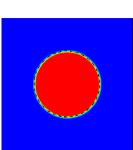
Figure 3: Steady-state density contours given by $M_{1}$ with ${s_{3}}=[1.0,1.4,1.8]$.

Let us denote ${\rho_{V}}$ and ${\rho_{L}}$ as the vapor and liquid coexistence densities, respectively. In this study, ${\psi_{0}}=1$, ${\rho_{0}}=1$ and $G=10/3$ are used, which leads to ${\rho_{V}}=0.3675$ and ${\rho_{L}}=2.783$ Yu and Fan (2009); Li et al. (2016b). The simulations are conducted in a periodic box $N\times N=200\times 200$. A circle droplet of radius $R$ is initialized by setting $\rho={\rho_{L}}$ in the circle and $\rho={\rho_{V}}$ outside the circle. The relaxation parameters are chosen as ${s_{b}}={s_{v}}=1.4$, and ${s_{3}}=[1.0,1.4,1.8]$.

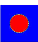
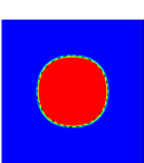
Figure 4: Steady-state density contours given by $M_{2}$ with ${s_{3}}=[1.0,1.4,1.8]$.

Figure 5: Steady-state density contours given by $M_{3}$ with ${s_{3}}=[1.0,1.4,1.8]$.

Firstly, the steady-state density contours with $R=50$ given by different forcing schemes are compared. The additional dashed circle represents the theoretical location of the droplet. It is found in Fig. 3 the shape of droplet is ${s_{3}}$-dependent and it changes from a out-of-round shape to a circle with the increase of ${s_{3}}$. As discussed in Sec. III.1, the removement of high-order terms for the central moments of $\Delta f$ in Premnath and Banerjee (2009) makes inconsistencies with the scheme proposed by Guo et al. And only when ${s_{3}}$ is set to be 2.0, the inconsistency can be eliminated. Though we can not give the result with ${s_{3}}=2.0$ (divergent for this simulation), the tendency confirms our argument. Anologously, as discussed in Sec. III.2 and Sec. III.3, the inconsistencies in $M_{2}$ and $M_{3}$ can only be eliminated under the conditions of ${s_{3}}={s_{2}}$ and ${s_{3}}=1.0$, respectively. Thus the droplets in Fig. 4 and Fig. 5 become out-of-round when ${s_{3}}$ is not set the specific value. For the present forcing scheme, the droplets are always in round shapes rather than depend on the value of ${s_{3}}$, as seen in Fig. 6.

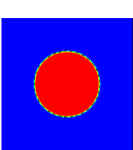
Figure 6: Steady-state density contours given by present method with ${s_{3}}=[1.0,1.4,1.8]$.

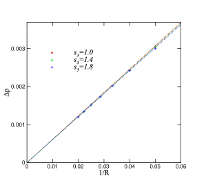
Figure 7: Numerical validation of Laplace’s law for the present forcing scheme.

According to Laplace’s law, the pressure difference between the pressure inside and the one outside a droplet is related to the surface tension $\gamma$ and the droplet radius $R$ via $\Delta p=\gamma/R$. To check the ability of repeating the Laplace’s law, a series of static droplets with $R=\left[{20,25,30,35,40,45,50}\right]$ are simulated. The pressure is computed through $p=\rho c_{s}^{2}+G{\psi^{2}}/2$. As shown in Fig. 7, Laplace’s law is well satisfied. The measured surface tensions for ${s_{3}}=[1.0,1.4,1.8]$ are 0.0615, 0.0610 and 0.0605, respectively.

V CONCLUSIONS

In this study, we present a more pellucid derivation of CLBM. A shift matrix ${\bf{N}}$ is defined in the derivation, by which the raw moments of the discrete distribution function are shifted to their central moments. This definition clarifies the relationship between the MRT LBM and CLBM. Based on this, a new method of incorporating forcing terms into the CLBM is proposed.

The forcing effect term is incorporated by means of central moments, which is compatible with the basic ideology of the CLBM. According to the definition of the shift matrix ${\bf{N}}$, the CLBM degrades into the MRT LBM when ${\bf{N}}$ is a unit matrix. The present forcing scheme retains the property of and degrades into the Guo forcing scheme in the MRT LBM when ${\bf{N}}$ is a unit matrix. Specifically, the present forcing scheme degrades to the original forcing schene proposed by Guo et al when all the relaxation parameters are set to the same. Numerical simulations for several benchmark problems confirm the applicability of the non-slip rule, the second-order accuray in space and the property of isotropy for the present scheme. In the meantime, some inconsistences in the previous models are also revealed.

The method developed is quite pellucid, and no cumbersome operations are involved in the practical implementation. Further work will demonstrate that the present scheme can be extended to three dimentions (3D) readily.

Appendix A Appendixes

Analogously, the raw moments can be transfromed to the discrete DF through ${\bf{M}}^{-1}$, and the central moments can be shifted to raw moments through ${\bf{N}}^{-1}$,

$$\begin{array}[]{l}\left|{{f_{i}}}\right\rangle={{\bf{M}}^{{\rm{-}}1}}\left|{{T_{i}}}\right\rangle,\\ \left|{{T_{i}}}\right\rangle={{\bf{N}}^{{\rm{-}}1}}\left|{{{\tilde{T}}_{i}}}\right\rangle.\\ \end{array}$$ (28)

The explicit expressions for ${\bf{M}}^{-1}$ and ${\bf{N}}^{-1}$ are

$${\bf{M}}^{-1}=\left[\begin{array}[]{c c c c c c c c c}1&0&0&-1&0&0&0&0&1\\ 0&1/2&0&1/4&1/4&0&0&-1/2&-1/2\\ 0&0&1/2&1/4&-1/4&0&-1/2&0&-1/2\\ 0&-1/2&0&1/4&1/4&0&0&1/2&-1/2\\ 0&0&-1/2&1/4&-1/4&0&1/2&0&-1/2\\ 0&0&0&0&0&1/4&1/4&1/4&1/4\\ 0&0&0&0&0&-1/4&1/4&-1/4&1/4\\ 0&0&0&0&0&1/4&-1/4&-1/4&1/4\\ 0&0&0&0&0&-1/4&-1/4&1/4&1/4\\ \end{array}\right],$$ (29)

and

$${\bf{N}}^{-1}=\left[\begin{array}[]{c c c c c c c c c}1&0&0&0&0&0&0&0&0\\ {u_{x}}&1&0&0&0&0&0&0&0\\ {u_{y}}&0&1&0&0&0&0&0&0\\ u_{x}^{2}+u_{y}^{2}&2{u_{x}}&2{u_{y}}&1&0&0&0&0&0\\ u_{x}^{2}-u_{y}^{2}&2{u_{x}}&-2{u_{y}}&0&1&0&0&0&0\\ {u_{x}}{u_{y}}&u_{y}&u_{x}&0&0&1&0&0&0\\ u_{x}^{2}{u_{y}}&2{u_{x}}{u_{y}}&u_{x}^{2}&{u_{y}}/2&{u_{y}}/2&2u_{x}&1&0&0\\ u_{y}^{2}{u_{x}}&{u_{y}}^{2}&2{u_{x}}{u_{y}}&{u_{x}}/2&-{u_{x}}/2&2u_{y}&0&1&0\\ u_{x}^{2}u_{y}^{2}&2{u_{x}}u_{y}^{2}&2{u_{y}}u_{x}^{2}&u_{x}^{2}/2+u_{y}^{2}/2&u_{y}^{2}/2-u_{x}^{2}/2&4{u_{x}}{u_{y}}&2{u_{y}}&2{u_{x}}&1\\ \end{array}\right].$$ (30)

References

- Qian et al. (1995) Y.-H. Qian, S. Succi, and S. Orszag, Annu. Rev. Comput. Phys 3, 195 (1995).
- Chen and Doolen (1998) S. Chen and G. D. Doolen, Annual review of fluid mechanics 30, 329 (1998).
- Succi (2001) S. Succi, The lattice Boltzmann equation: for fluid dynamics and beyond (Oxford university press, 2001).
- Shan and Chen (1993) X. Shan and H. Chen, Physical Review E 47, 1815 (1993).
- Guo and Shu (2013) Z. Guo and C. Shu, Lattice Boltzmann method and its applications in engineering, Vol. 3 (World Scientific, 2013).
- Gong et al. (2016) W. Gong, Y. Zu, S. Chen, and Y. Yan, Science Bulletin 62, 136 (2016).
- Li et al. (2016a) Q. Li, K. Luo, Q. Kang, Y. He, Q. Chen, and Q. Liu, Progress in Energy and Combustion Science 52, 62 (2016a).
- Qian et al. (1992) Y. Qian, D. d’Humières, and P. Lallemand, EPL (Europhysics Letters) 17, 479 (1992).
- d’Humieres (1994) D. d’Humieres, Rarefied gas dynamics- Theory and simulations , 450 (1994).
- Geier et al. (2006) M. Geier, A. Greiner, and J. G. Korvink, Physical Review E 73, 066705 (2006).
- Lallemand and Luo (2000) P. Lallemand and L.-S. Luo, Physical Review E 61, 6546 (2000).
- Lycett-Brown and Luo (2016) D. Lycett-Brown and K. H. Luo, Physical Review E 94, 053313 (2016).
- Fei and Luo (2016) L. Fei and K. Luo, arXiv preprint arXiv:1610.07114 (2016).
- Ginzburg (2005) I. Ginzburg, Advances in Water resources 28, 1171 (2005).
- Ginzburg et al. (2008) I. Ginzburg, F. Verhaeghe, and D. d’Humieres, Communications in computational physics 3, 427 (2008).
- Ansumali et al. (2003) S. Ansumali, I. V. Karlin, and H. C. Öttinger, EPL (Europhysics Letters) 63, 798 (2003).
- Ansumali and Karlin (2000) S. Ansumali and I. V. Karlin, Physical Review E 62, 7999 (2000).
- He et al. (1999) X. He, S. Chen, and R. Zhang, Journal of Computational Physics 152, 642 (1999).
- Buick and Greated (2000) J. M. Buick and C. A. Greated, Physical Review E 61, 5307 (2000).
- Ladd and Verberg (2001) A. Ladd and R. Verberg, Journal of Statistical Physics 104, 1191 (2001).
- Guo et al. (2002) Z. Guo, C. Zheng, and B. Shi, Physical Review E 65, 046308 (2002).
- Guo and Zheng (2008) Z. Guo and C. Zheng, International Journal of Computational Fluid Dynamics 22, 465 (2008).
- Premnath and Banerjee (2009) K. N. Premnath and S. Banerjee, Physical Review E 80, 036702 (2009).
- Lycett-Brown and Luo (2014) D. Lycett-Brown and K. H. Luo, Computers & Mathematics with Applications 67, 350 (2014).
- De Rosis (2017a) A. De Rosis, Physical Review E 95, 023311 (2017a).
- Asinari (2008) P. Asinari, Phys Rev E 78, 016701 (2008).
- Liu et al. (2016) Q. Liu, Y.-L. He, D. Li, and Q. Li, International Journal of Heat and Mass Transfer 102, 1334 (2016).
- He et al. (1998) X. He, S. Chen, and G. D. Doolen, Journal of Computational Physics 146, 282 (1998).
- Ginzburg and d’Humières (2003) I. Ginzburg and D. d’Humières, Physical Review E 68, 066614 (2003).
- Kupershtokh et al. (2009) A. Kupershtokh, D. Medvedev, and D. Karpov, Computers & Mathematics with Applications 58, 965 (2009).
- Huang et al. (2011) H. Huang, M. Krafczyk, and X. Lu, Physical Review E 84, 046710 (2011).
- Li et al. (2012) Q. Li, K. H. Luo, and X. J. Li, Physical Review E 86, 016709 (2012).
- Lycett-Brown and Luo (2015) D. Lycett-Brown and K. H. Luo, Physical Review E 91, 023305 (2015).
- Freitas et al. (2011) R. K. Freitas, A. Henze, M. Meinke, and W. Schröder, Computers & Fluids 47, 115 (2011).
- Taylor (1934) G. Taylor, Proceedings of the Royal Society of London. Series A, Containing Papers of a Mathematical and Physical Character 146, 501 (1934).
- De Rosis (2017b) A. De Rosis, EPL (Europhysics Letters) 116, 44003 (2017b).
- Yu and Fan (2009) Z. Yu and L.-S. Fan, Journal of Computational Physics 228, 6456 (2009).
- Li et al. (2016b) Q. Li, P. Zhou, and H. Yan, Physical Review E 94, 043313 (2016b).