From bare to renormalized order parameter in gauge space: structure and reactions

Abstract

The physical reason why one can calculate with similar accuracy, as compared to the experimental data, the absolute cross section associated with two-nucleon transfer processes between members of pairing rotational bands, making use of simple BCS (constant matrix elements) or of many-body (Nambu-Gorkov (NG), nuclear field theory (NFT)) spectroscopic amplitudes, is not immediately obvious. Restoration of spontaneous symmetry breaking and associated emergent generalised rigidity in gauge space provides the answer, and points to a new emergence: a physical sum rule resulting from the intertwining of structure and reaction processes and closely connected with the central role induced pairing interaction plays in structure together with the fact that successive transfer dominates Cooper pair tunnelling.

today

I Introduction

The starting point of most descriptions of nuclear structure and reactions is based on independent particle motion. The validity of such a picture is related to basic quantum mechanics. Potential energy privileges fixed position between particles. Fluctuations, in particular quantum fluctuations, the only ones operative in a nucleus in its ground state, symmetries. Regarding single-particle motion, such competition is embodied in the quantality parameter Mottelson1998 ,

$$q=\frac{\hbar^{2}}{ma^{2}}\frac{1}{|v_{0}|},$$ (1)

where $m$ is the nucleon mass, $v_{0}$ and $a$ being the strength and the range of the strong NN-potential respectively ($v_{0}\approx-100$ MeV, $a\approx$ 1 fm). The above equation is the ratio between the kinetic energy of confinement and the potential energy. Because $q\approx 0.4$, nucleons in the nucleus are delocalized, and mean field is a good approximation. In particular, the HF mean field.

II Spontaneous symmetry breaking

The fact that basic properties of a quantal system can be described in terms of a mean field solution which does not display some of the symmetries of the original Hamiltonian is the spontaneous symmetry breaking phenomenon.

The lower symmetry mean field solution defines a privileged orientation in the corresponding three-dimensional (e.g. Nilsson) , gauge (e.g. BCS, HFB) , etc. space. All orientations have the same energy, in keeping with the fact that the restoring constant associated with changes in the Euler-, gauge-, etc. angles is zero. Fluctuations in orientation thus diverge in precisely the right manner to restore symmetry (see e.g. Brink2005 , Sects. 4.2. and 4.2.3 and refs. therein). Because this divergence is associated with the vanishing of the frequency for constant inertia, the system acquires generalised rigidity (emergent property). Thus, acting with the specific external field (Cooper pair transfer in the case of pairing rotational band), sets the deformed system into rotation as a whole, without retardation effects. The above phenomena are at the basis of the broken symmetry restoration paradigm used to identify the elementary modes of nuclear excitation (see e.g. Bohr1975 and refs. therein). In particular pairing rotations Bohr1975 ; Bes1966 ; Broglia2016 ; Broglia2000 ; Hinohara2016 ; Lopez:13 .

Pairing in nuclei has been introduced a number of times. The first to explain the enhanced stability of even as compared to odd nuclei Heisenberg1932 . Subsequently, to describe the correlations associated with such staggering effects Mayer1950 ; Racah1952 . After the BCS explanation of superconductivity Bardeenetal1957a ; Bardeenetal1957b , to account for the presence of a gap in the low-energy intrinsic excitation spectrum of deformed nuclei Bohr1958 . Finally, in connection with the advent of the Josephson effect, namely Cooper pair tunnelling, and the study of two–nucleon transfer processes, specific probes of deformation in gauge space Bohr1964 ; Yoshida1962 .

II.1 Order parameter of nuclear superfluid phase

The order parameter associated with independent pair motion is defined as,

$$\alpha^{\prime}_{0}=\langle BCS(N+2)|P^{\prime+}|BCS(N)\rangle,$$

$$=\sum_{j}\sqrt{\frac{2j+1}{2}}B(j^{2}(0),N\to N+2).$$ (2)

That is, the number of pairs participating in the BCS condensate. The quantity

$$B(j^{2}(0),N\to N+2)=\langle BCS(N+2)|T^{\prime+}(j^{2}(0))|BCS(N)\rangle,$$

$$=\sqrt{\frac{2j+1}{2}}U^{\prime}_{j}(N)V^{\prime}_{j}(N+2),$$ (3)

is the two-nucleon transfer spectroscopic amplitude,

$$T^{\prime+}(j^{2}(0))=\frac{[{a^{\prime}_{j}}^{+}{a^{\prime}_{j}}^{+}]_{0}}{\sqrt{2}},$$ (4)

being the two-nucleon (Cooper pair) transfer operator, while

$$P^{\prime+}=\sum_{jm>0}{a^{\prime}_{jm}}^{+}{a^{\prime}_{\bar{jm}}}^{+}=\sum_{j}\sqrt{\frac{2j+1}{2}}T^{\prime}(j^{2}(0)),$$ (5)

is the operator which creates a pair of particles in time reversal states. $|BCS(N)\rangle$ labels the BCS state for which the $\lambda$ parameter (Fermi energy) has been adjusted so that 2$\sum_{jm>0}{V^{\prime}_{j}}^{2}=N.$

In keeping with (2), the order parameter $\alpha^{\prime}_{0}=\sum_{j}\left(\frac{2j+1}{2}\right)U^{\prime}_{j}(N)V^{\prime}_{j}(N+2)\approx\sum_{j}\left(\frac{2j+1}{2}\right)U^{\prime}_{j}V^{\prime}_{j}$ provides a measure of the nuclear deformation in gauge space, and thus of the fact that the system displays a privileged orientation in this space, as can be seen from the relation (see App. A)

$$\alpha^{\prime}_{0}=\sum_{j}\left(\frac{2j+1}{2}\right)U^{\prime}_{j}V^{\prime}_{j}=e^{2i\phi}\sum_{j}\left(\frac{2j+1}{2}\right)U_{j}V_{j}=e^{2i\phi}\alpha_{0},$$ (6)

where the primed quantities are the BCS occupation amplitudes referred to the intrinsic system of reference in gauge space (i.e. body-fixed BCS state), while the unprimed quantities are the same quantities referred to the laboratory system of reference. The two systems are connected by a rotation in gauge space of angle $\phi$, induced by the operator ${\cal G}=exp(-i\hat{N}\phi)$, $\hat{N}$ being the number operator and thus $a^{\prime+}_{jm}={\cal G}(\phi)a^{+}_{jm}{\cal G}^{-1}(\phi)$ (see e.g. Poteletal2013 and refs. therein).

A simple empirical confirmation that $\alpha_{0}$ is the number of Cooper pairs of a superfluid nucleus can be made with the help of the single $j-$shell model. In this model $V_{j}=(N/2\Omega)^{1/2}$ and $U_{j}=(1-N/2\Omega)^{1/2}$, where $\Omega=(2j+1)/2$. For a system with $N=\Omega$ particles, i.e. $\Omega/2$ pairs, half filled shell, typical of a superfluid nucleus, $V_{j}=U_{j}=(1/2)^{1/2}$ and $\alpha_{0}=\Omega/2$. Thus, $\alpha_{0}$ gives an estimate of the number of Cooper pairs which participate in specifying the orientation the $|BCS\rangle$ state has in gauge space. With the help of the approximate expression $\Omega=(2/3)A^{2/3}$ one obtains, for ¹²⁰Sn, $\alpha_{0}=8$. Detailed microscopic calculations give values of $\alpha_{0}=5-6$ (see Sect.VI Table 2).

Symmetry restoration results from zero point fluctuations of the gauge angle setting the BCS deformed state into rotation and leading to pairing rotational bands, e.g. the ground state of superfluid Sn-isotopes, where $N$ plays, in gauge space, the role angular momentum plays in quadrupole rotational motion. This symmetry restoration can be implemented by diagonalizing in QRPA the residual interaction $H_{res}$ acting among quasiparticles and neglected in the BCS mean field approximation (cf. App. A).

Because there are two parameters which determine the admixture of particle and hole states connected with gauge symmetry breaking, namely $U_{j}$ and $V_{j}$ (quasiparticle transformation), there are only two fields $F$ which contribute to $H_{res}$ through terms of the type $FF^{+}$. One, antisymmetric with respect to the Fermi energy, namely $U_{j}^{2}-V_{j}^{2}$ and leading to pairing vibrations of the gauge deformed state $|BCS\rangle$ ($H^{\prime}_{p}$ contribution to $H_{res}$, cf. e.g. Brink2005 , App. J). The other one, ${U_{j}}^{2}+{V_{j}}^{2}$ is symmetric with respect to $\epsilon_{F}$ and leads to fluctuations which restore gauge symmetry ($H^{\prime\prime}_{p}$ contribution to $H_{res}$, $H_{BCS}+H^{\prime\prime}_{p}$ commute with $\hat{N}$). Within this scenario, the field $U_{j}^{2}-V_{j}^{2}$ excites two-quasiparticle states. Eliminating (in a particle-conserving fashion) this contribution from $U_{j}^{2}+V_{j}^{2}$, one obtains the field which connects the members of a ground state rotational bands. That is $((U^{2}_{j}+V^{2}_{j})^{2}-(U^{2}_{j}-V^{2}_{j})^{2})^{1/2}\sim U_{j}V_{j}$. This result, together with (3) and (4), testifies to the fact that two-nucleon transfer reactions are, from the point of view of structure, the specific probes of pairing condensation in nuclei Poteletal2013a , as it emerges in a natural fashion writing

$$\alpha_{0}=\langle BCS|\sum_{j}\left(\frac{2j+1}{2}T(j^{2}(0))\right)|BCS\rangle$$ (7)

It is then natural that the absolute two-nucleon transfer cross section between members of a pairing rotational band can, schematically, be written as

$$\sigma\sim|\alpha_{0}|^{2},$$ (8)

emphasizing again the close connection (unification) of structure and reaction aspects of the subject under discussion.

III Physical nucleons and induced pairing

In what follows we will show that there is a simple physical reason at the basis of the above parlance, rooted on the fact that the atomic nucleus is a leptodermous finite many-body quantal system. Virtual states, like those associated with zero-point fluctuations (ZPF) of the nuclear vacuum (ground state), e.g, in which a surface quantised vibration and an uncorrelated particle-hole mode get virtually excited for a short period of time (Fig. 1, I(a)) are a basic characterising feature of these systems Baroni . Adding a nucleon to it (odd system, Fig. 1 (I) (b)) leads, through the particle–vibration coupling strength ($V$, (see e.g. Schuck Eq. (C6))) to processes which contain the effect of the antisymmetry between the single-particle explicitly considered and the particles out of which the vibrations are built (Fig. 1 (I)(c)). Time ordering gives rise to the graph shown in Fig. 1 (I)(d). Processes I(c) and I(d) known as correlation (CO) and polarisation (PO) contributions to the mass operator (see Mahaux and refs. therein) cloth the particles, leading to physical nucleons whose properties can be compared with the experimental findings. Summing up, the processes shown in Fig. 1 (I) are textbook examples of quantal nuclear phenomena testifying to the fact that the clothing of nucleons is at the basis of the quantal description of the atomic nucleus.

Nuclear superfluidity at large, and its incipience in the case of single Cooper pair like e.g. in ¹¹Li in particular, are among the most quantal of all the phenomena displayed by the nuclear many-body system. Even if the ${}^{1}S_{0}$, $NN-$interaction was not operative, or was rendered subcritical by screening effects as in the case of ¹¹Li, Cooper binding will still be healthy, as a result of the exchange of vibrations between pairs of physical (clothed) nucleons moving in time reversal states close to the Fermi energy (Fig. 1 (II)(b),(d)-(g)), a direct consequence of the ZPF of the nuclear vacuum (ground state) (Fig. 1 (I)(a) and (c))

Within this context, and only so, is that one can posit that the order parameter $\alpha_{0}$ does not depend on the presence or less of the ${}^{1}S_{0}$, $NN-$bare potential. Independent Cooper pair motion and thus nuclear superfluidity is intrinsically contained in the fluctuations of the quantal nuclear vacuum. As such, it is a truly emergent many-body nuclear property implying generalised rigidity in gauge space, the associated pairing rotational bands being specifically excited through pair transfer Bes1966 ; Broglia2000 ; Hinohara2016 . The fingerprint of spontaneous symmetry breaking in finite many-body systems is the presence of rotational bands associated with symmetry restoration. To qualify as a rotational band, a set of levels must display enhanced transition probabilities (absolute cross sections), associated with the operator having a non-vanishing value in the (degenerate) ground state (order parameter). In the present case (pairing rotational bands), of the two-nucleon transfer operator Poteletal2013 ; BrogliaHansenRiedel . In other words, cross talk (absolute transfer cross sections) between a member of a pairing rotational band and states not belonging to it, should be much smaller than between members of the band. It could be argued that also important for the characterisation of a pairing rotational band is the parabolic dependence of the energy with particle number. True, but many non-specific aspects can modify this dependence, without altering the gauge kinship (common $|BCS\rangle$ like intrinsic state). Before adscribing to two-nucleon transfer processes the role of specific probe not only from the point of view of nuclear structure, but also from the vantage point of nuclear reactions , a subject concerning the reaction mechanism is to be clarified.

Making use of the fact that in superfluid nuclei lying along the stability valley like e.g. the Sn-isotopes, about half of the neutron pairing gap is associated with the induced pairing interaction EPJ ; Idini2015 , that is, $\Delta_{ind}\approx g_{pv}\alpha_{0}=\Delta_{exp}/2\approx 0.8$ MeV, where $g_{pv}$ is the particle-vibration coupling parameter (equal to minus the induced pairing interaction), and of the fact that the mass enhancement factor $\lambda$ (i.e. $m_{\omega}=m(1+\lambda)\approx 1.4m$, see e.g. Mahaux , see also Schuck Eq (C11)) can be written as $\lambda=g_{pv}N(0)(\approx 0.4)$, one obtains (see App. E)

$$N(0)\approx\frac{1}{2}\alpha_{0}\;{\rm MeV}^{-1}\approx 4\;{\rm MeV}^{-1},$$ (9)

for the density of neutron levels of e.g. ${}^{120}_{50}$Sn_t0 at the Fermi energy and for one spin orientation, as experimentally observed ($a\approx N/8$ MeV^-1 for both spin orientation, see Bortgdr , Eq (7.16)).

As a consequence of Eqs. (8) and (9),

$$\sigma\sim(N(0))^{2}.$$ (10)

In other words, Cooper pair tunneling in nuclei is dominated by successive transfer. The significance of this result becomes clearer by recalling the fact that according to the golden rule, to processes like tunneling or decay is associated a decay width linear in the density of states.

One can then argue that successive transfer may imply pair breaking, making two-nucleon transfer reactions a less than ideal probe of pairing correlations in nuclei. That this is not so can be understood by calculating the correlation length, that is, the range over which Cooper pairs partners, correlated by the exchange of collective vibrations, feel the presence of each other. One obtains (see App. F)

$$\xi_{ind}=\frac{\hbar v_{F}}{\pi\Delta_{ind}}=\frac{\hbar v_{F}}{\pi g_{pv}\alpha_{0}}=\frac{\hbar v_{F}N(0)}{\pi\lambda\alpha_{0}}\approx 24\;{\rm fm}.$$ (11)

On carrying out the above estimate use has been made of $v_{F}/c=0.3$, $\lambda=0.4$ and $\alpha_{0}=8$. As a result, the generalised pair quantality parameter

$$q_{\xi_{ind}}=\frac{\hbar^{2}}{(2m)\xi_{ind}^{2}}\frac{1}{g_{pv}\alpha_{0}}\approx\frac{\hbar^{2}}{2m\xi_{ind}^{2}}\frac{N(0)}{\lambda\alpha_{0}}\approx 0.04,$$ (12)

has a value much smaller than 1, implying potential energy dominance and thus to a strong correlation of the two partner nucleons of the Cooper pair over distances of the order of $\xi$, quantity larger than nuclear dimensions. This result testifies to the fact that successive transfer of nucleons fully probes the nuclear pair correlations.

The wave function of the nucleons in the pair are phase–coherent, so one has to add the transfer amplitudes before taken the modulus square. The nucleons do not tunnel independently, but more like a single particle, and the probability of a pair going through is comparable to the probability for a single nucleon. It is like interference in optics with phase-coherent wave mixing. In a nutshell, and denoting $P_{1}$ and $P_{2}$ the single and pair nucleon transfer probability , one can write

$$P_{2} =\left|\frac{1}{\sqrt{2}}\left(e^{i\phi^{\prime}}U\sqrt{P_{1}}+e^{i\phi}V\sqrt{P_{1}}\right)\right|^{2}=P_{1}\frac{(1+2UV\cos\epsilon)}{2}\approx P_{1}$$

$$\quad(\epsilon\equiv\phi-\phi^{\prime}),$$ (13)

where the assumption was made that $\epsilon=0$ and $U=V=1/\sqrt{2}$, in keeping with the fact that the “single particle” pair wavefunction is $(U_{\nu}+V_{\nu}e^{-i2\phi}a^{+}_{\nu}a^{+}_{\bar{\nu}})|0\rangle$, and of the single–$j$ shell estimate of the BCS occupation amplitudes.

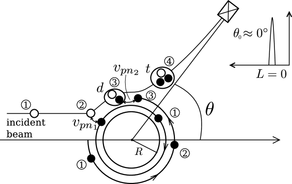
Figure 2: Schematic representation of Cooper pair transfer in the reaction ¹²⁰Sn$(p,t)^{118}$Sn (gs) leading to essentially a single peak in the spectrum at $0^{\circ}$ (after Poteletal2013a Fig 1 (II) (b) and (c)).

Summing up, in the reaction ¹²⁰Sn +p $\to$ (¹¹⁹Sn + d) $\to$ ¹¹⁸Sn + t, the first neutron of the Cooper pair picked up by the proton to constitute the (virtual) deuteron can be at the surface of the nucleus close to the proton, while the second one can be at the antipode (diameter $\approx$ 12 fm), eventually the second one being transferred to form the triton within the interaction range ($\approx$ 2 fm). This scenario involves relative distances between the partners of a Cooper pair, one in the target the other one in the (virtual) deuteron, of the order of 10-14 fm (see Fig. 2, where the inner $(n_{1})$ orbital motion is to be interpreted to schematically describe clockwise motion, the external one ($n_{2}$), anticlockwise one). Thus transfer of a rather extended object made out of two neutrons moving in time reversal states, still correlated as a single–particle of mass $2m^{*}$, in keeping with the estimated value of $\xi$ and of the phase coherence expressed by the relation $P_{2}\approx P_{1}$.

Following practice we refer throughout this paper to structure and reactions as two separate issues in the study of the atomic nucleus. While likely pedagogic, such an approach is fundamentally wrong as already suggested in the abstract. In a nutshell, structure and reactions are two aspects of the same subject. One likely involving bound the other continuum states, a distinction which is not even operative universally, certainly not in the case of light exotic halo nuclei. But more important, because in quantum mechanics one can hardly call physical a non measurable feature of a system.

Within this context, the quantity (6) modulus squared cannot be measured, but only when each of its terms are properly weighted by the formfactors (i.e. successive as well as simultaneous and non–orthogonality functions), and energy denominators (Green functions), as forcefully expressed in (7) (see also Poteletal2013a , App A in particular Eq. (A.21), Poteletal2013 Sect. III specially Eq. (38 (b)) as well as Physica_scripta , Figs. 2 and 12). Consequently, when discussing about the order parameter $\alpha_{0}$, in particular concerning the possible emergence of a physical sum rule, we are all the time aware of this fact even if, for simplicity, we do not state it explicitly. In other words, talking about $|\alpha_{0}|^{2}$ the ultimate reference is to the results displayed in Figs 4 and 5, namely predicted observables (absolute differential cross section) in comparison with the experimental findings. This implies that each term of $\alpha_{0}$ has to be viewed as the weighted $j^{2}(0)$, mainly successive, formfactor associated with independent pair motion, in a similar way in which, talking about one–nucleon transfer, independent particle motion implies a spectroscopic amplitude and a radial formfactor, also renormalized if that is the case (see e.g. 11Be and refs. therein). While the results contained in Table 1 and 2 play an important role in the calculation of observables, the different entries still refer to the assessment of theory against theory.

With the above proviso we can state that in keeping with the fact that $|BCS\rangle$ is a coherent state, displaying off diagonal long range order (ODLRO, see Apps. A, B and C), one expects (8) to be a physically conserved quantity. Also that the robustness of the order parameter $\alpha_{0}$ to characterise nuclear superfluidity as compared to the pairing gap is testified by the fact that $\alpha_{0}$ is different from zero also in nuclear regions, like between two heavy ions at the distance of closest approach in e.g. the process $a(=b+2)+A\to b+B(=A+2)$, situation in which the pairing interaction and thus also $\Delta$ are zero.

Let us conclude this Section by noting that while the expression (III) displays in a simple way the gauge phase coherence associated with independent pair motion, it does not contain the independent particle limit, lacking the energy denominator. This limit is of course simple to exhibit in the quantal Poteletal2013 or semiclassical Poteletal2013a formalism mentioned above, which has the backdraw of becoming involved in connection with phase gauge coherence.

Figure 1: (I) (a) ZPF associated with (particle-hole) surface vibrations; (b) odd system; (c) the antisymmetrization between the particles considered explicitly and those involved in the vibration; (d) time ordering of (c). Diagrams (c) and(d) lead to the clothing of single-particle motion in lowest order in the particle-vibration coupling vertex. (II) A dressed nucleon moving in a state $\nu$ in the presence of: (a) a bare nucleon moving in the time reversed state $\bar{\nu}$, (c) another dressed nucleon. Exchange of vibration in $(a)$ leads to (b), the NFT lowest-order contribution in the particle-vibration coupling vertex, of the induced pairing interaction (App. G). Exchange of vibrations in (c) leads to (d) self-energy, (e) vertex correction of the induced pairing interaction (App. H); (f) ladder diagram contributing to the induced pairing interaction. The symmetrisation between the bosons displayed in (c) is shown in (g).

IV Many-body aspects of the nuclear pairing interaction

While in condensed matter the many-body aspects of the pairing interaction could not be ignored, this could happen in nuclear physics. This is primarily due to the fact that the electron-electron bare interaction is repulsive (Coulomb). But also because of the fact that the highest values of $T_{c}$ in low-temperature metallic superconductors are, as a rule, associated with bad conductors at room temperature , underscoring the role played by the electron-phonon coupling in the superconducting phenomenon, and the need for a correct treatment of this interaction. In other words, the scenario of the Nambu–Gorkov and Eliashberg approach to superconductivity Gorkov ; Nambu ; Eliashberg .

In nuclear physics, on the other hand, the values of ${}^{1}S_{0}$ phase shifts are positive for low values of the relative nucleon velocities ($E_{lab}\leq$ 200 MeV), let alone the fact that the particle-vibration coupling mechanism is still often thought to give only rise to self-energy phenomena. As a result, it was assumed that the nuclear pairing interaction was short range and resulting solely from meson exchange, long range interactions being responsible for mean field effects (see e.g. Bessorensen and refs. therein), an attitude which has proven to be difficult to overcome. In other words, similarly to the fact that one cannot measure the bare nucleon mass in nuclei but the clothed one (see Fig. 1 (I)(c),(d)), one cannot measure the bare pairing interaction in the nuclear medium but the effective one, sum of the bare ($v^{p}_{bare}$) and of the induced ($v_{p}^{ind}$) one (see Fig. 1 (II)(b),(d)-(g)). Furthermore, in nuclear physics as in condensed matter, a non–perturbative treatment of the PVC is needed in a number of cases, e.g. in connection with the breaking of the $d_{5/2}$ orbit of ¹²⁰Sn.

Applying, within the framework of NFT, the Nambu-Gorkov technique developed to describe metallic superconductors to this open shell nucleus, it is possible to obtain a complete characterization of it. The theoretical predictions reproduce the experimental results within the 10% level Idini2015 . As we shall see below, the contributions of the many-body effects related to the one-particle channel do not affect the absolute two-nucleon transfer reaction cross section in any major way. This fact testifies to the robustness of $\alpha_{0}$, in the sense of two–nucleon transfer spectroscopic amplitude as explained in Sect. III, and to the physical soundness to make it the nuclear superfluid order parameter.

V Elementary modes of excitation: empirical renormalization in structure and reactions

The elementary modes of excitation of a many-body system represent a generalization of the idea of normal modes of vibration. They constitute the building blocks of the excitation spectra, providing insight into the deep nature of the system one is studying, aside from allowing for an economic description of complicated spectra in terms of a gas of, as a rule, weakly interacting bosons and fermions. In the nuclear case they correspond to clothed particles and empirically renormalised vibrations (rotations).

There lie two ideas behind the concept of elementary modes of excitation. First, that one does not need to be able to calculate the total binding energy of a nucleus to accurately describe the low energy excitation spectrum, in much the same way in which one can calculate the normal modes of a metal rod not knowing how to calculate its total cohesive energy. The second idea is that low-lying states ($\hbar\omega\ll\epsilon_{F}\ll BE)$ are of a particularly simple character, and are amenable to a simple treatment, their interweaving being carried out at profit, in most cases, in perturbation theory . Within this context it is necessary to have a microscopic description of the ground state of the system which ensures that it acts as the vacuum state $|\tilde{0}\rangle$ of the elementary modes of excitation. In other words $a_{\nu}|\tilde{0}\rangle=0,\Gamma_{\alpha}|\tilde{0}\rangle=0$, where $a^{+}_{\nu}|\tilde{0}\rangle=|\nu\rangle$ and , $\Gamma^{+}_{\alpha}|\tilde{0}\rangle=|\alpha\rangle$ represent a single-particle and a one-phonon state. This implies, in keeping with the indeterminacy relations $\Delta x\Delta p\geq\hbar/2$, that $|\tilde{0}\rangle=|0\rangle_{F}|0\rangle_{B}$ displays quantal zero point fluctuations (ZPF).

Within the framework of nuclear field theory (NFT) used below, in which single-particle (fermionic, F) and vibrational (bosonic, B) elementary modes of excitation are to be calculated within the framework of HFB and QRPA respectively, $|\tilde{0}\rangle$ must display the associated ZPF (cf. App. D). In particular for (harmonic) vibrational modes $\Delta x\Delta p=\hbar/2$, the associated zero point energy amounting to $\hbar\omega/2$ for each degree of freedom, e.g 5$\hbar\omega/2$ for quadrupole vibrations, $\hbar\omega$ being the energy of the collective vibrational mode under consideration.

An illustrative example of the above arguments is provided by the low-lying quadrupole vibrational state of ¹²⁰Sn. Diagonalizing SLy4 in QRPA leads to a value of $B(E2)$ (890 $e^{2}$ fm²) which is about a factor of 2 smaller than experimentally observed (2030 $e^{2}$ fm²). Taking into account renormalisation effects in NFT, namely in a conserving approximation (self-energy and vertex corrections, generalised Ward identities), one obtains a value (2150 e² fm ²), which essentially coincides with the experimental findings. One does not know how to accurately calculate the absolute ground state energy $E_{0}$ (total binding energy) of e.g. ¹²⁰Sn, but one can do pretty well to work out the properties of the low-energy mode of this nucleus, also the collective energies $\hbar\omega_{L}=E_{L}-E_{0}$, and thus the associated ZPF and zero point energy $E_{0}$, by renormalizing QRPA solutions to lowest order through self-energy and vertex corrections contributions EPJ . Now, if the collective phonons are not the main object of the study, but are to be used to cloth the single-particle states and give rise to the induced pairing interaction, one can make use of phonons which account for the experimental findings (empirical renormalization Idini2015 , see also Physica_scripta ; 11Be ).

It is to be noted that in calculating the $E\lambda$ lifetimes , e.g. the quadrupole lifetime associated with the low-lying quadrupole mode $(T(E2)=1.22\times 10^{9}\times E_{\gamma}^{5}\times B(E2),\;E_{\gamma}=\hbar\omega_{2^{+}}$), the kinematic ($E_{\gamma}^{5})$ and structure ($B(E2)$) contributions can be treated separately. This is in keeping with the fact that in the case of electromagnetic decay as well as of anelastic processes, the relative motion coordinate is always that of the entrance channel, at variance with particle transfer processes. Consequently, in connections with these processes, structure and reactions are treated separately, a possibility not operative in the case of transfer reactions. Let us extend this discussion to particle transfer process. In particular, to the two-particle pickup reaction ¹²⁰Sn(p,t)¹¹⁸Sn(gs). In this case, and to be able to calculate the radial dependence of successive transfer, everything has to be translated in terms of single-particle motion and associated absolute separation energies and radial wave functions in systems with different relative coordinates.

If the $k-$mass connected with the Perey-Buck energy-dependent term Mahaux already made the concept of a single mean field potential somewhat illusory (App. E), consider the difficulties one is confronted with in attempting at translating into a single-particle motion description inside a common potential, independent motion of Cooper pairs, composite bosonic particles with binding energies of the order of one tenth of the Fermi energy ($\approx 2\Delta/\epsilon_{F}\approx$ 3 MeV/36 MeV) and a correlation length of tens of fm, subject to a strong external field of radius $R_{0}\approx$ 6 fm and depth $\approx 50$ MeV. A way out to this situation is provided by the fact that in superfluid nuclei, one is not very far from an independent particle picture. As a consequence, no major errors are introduced in treating the system accordingly. Also in keeping with the fact that transfer takes place through the single-particle field Poteletal2013 .

Summing up, while one does not know how to calculate the mass of the nucleus, one can accurately calculate $U_{j}(118)V_{j}(120)$, as well as the relative value of the clothed single-particle energies. In keeping with the fact that renormalised NFT which makes use of NG equation correctly reproduces the quasiparticle energies, the Fermi energy of the single-particle potential used to generate the radial wave function is adjusted so that the least bound state has the experimental separation energy $S_{n}$. Within the unified picture of structure and reactions (NFT (r+s), Physica_scripta ), dressing f the radial wavefunctions give rise to the correct formfactors for transfer processes. While these effects are small for ¹²⁰Sn, there are overwhelming in other situations, e.g. that of halo nuclei 11Be .

VI Cooper pair population of pairing rotational bands: BCS,HFB and NG

In what follows we analyse the stability of the order parameter as probed by Cooper pair transfer.

VI.1 BCS

Starting from a HF calculation with the SLy4 interaction (Table 1, second column) we solve the BCS equations, and thus determine the corresponding occupation numbers $U_{a}(G)$ and $V_{a}(G)$ (Table 1, last two columns) with a schematic monopole pairing force of strength $G=0.26$ MeV, adjusted to fit the empirical three-point value $\Delta^{exp}\approx 1.4$ MeV.

VI.2 HFB

Making use of the same Skyrme interaction and of the $v_{14}$ Argonne, ${}^{1}S_{0}$ NN-potential and neglecting the influence of the bare pairing force in the mean field, the HFB equation was solved. As a result, this step corresponds to an extended BCS calculation over the HF basis, allowing for the interference between states of equal quantum numbers $a(\equiv lj)$, but different number of nodes $(k,k^{\prime})$. We include $(N_{a})$ states (for each $a$) up to $\approx$1 GeV, to properly take into account the repulsive core of $v_{14}$ and be able to accurately calculate $\Delta^{HFB}$. As a consequence, one obtains a set of quasiparticle energies $E^{\mu}_{a}$, with the quasiparticle index $(\mu=1,2...N_{a})$. To each quasiparticle $\alpha^{+}_{a,\mu}=\sum_{k=1}^{N_{a}}(U_{a}^{\mu,k}a^{+}_{a,k}-V_{a}^{\mu,k}a_{a,k})$ is associated an array of quasiparticle amplitudes $U_{a}^{\mu,k}$ and $V_{a}^{\mu,k}$ which are the components of the quasiparticles over the HF basis states $\phi^{a}_{k}=\langle\vec{r}|a^{+}_{a,k}|0\rangle(\equiv\langle\vec{r}|a,k\rangle).$ Going to the canonical basis, where the density matrix takes a diagonal form, we look for the state having the largest value of the abnormal density, $(UV)_{max}$. As a rule, for a well-bound nucleus such as ¹²⁰Sn, this canonical state is the quasiparticle state having the lowest value of the quasiparticle energy. The label $k$ then drops because there is only one orbital for a given value of $a(\equiv(lj))$. This implies that the bare quasiparticle amplitudes can be characterised simply by $U_{a},V_{a}$ and the associated state dependent value of the bare pairing gap is equal $\Delta^{bare}_{a}=2U_{a}V_{a}E_{a}$. The values of $(E_{a})_{min}$ and $(V_{a}(v_{14}))_{max}$ for the five valence orbitals are reported in Table 1.

VI.3 Renormalized NFT and NG

We now go beyond mean field and include the particle-vibration coupling leading to retardation phenomena both in self energy as well as in induced interaction processes. The vibrational modes are calculated in QRPA making use of empirical (WS) single–particle levels, BCS with constant $G$ and multipole–multipole separable interactions of essentially self–consistent strength Bohr1975 which reproduce the observed properties of the low–lying collective states.

To be able to treat the variety of possible situations we return to the full HFB basis. In this basis the $\omega-$dependent self energy has the following matrix structure Idini_tesi ,

$$\hat{\Sigma}^{a}_{\mu,\mu^{\prime}}(\omega)=\left(\begin{array}[]{c c}\Sigma^{11,a}_{\mu,\mu^{\prime}}(\omega)&\Sigma^{12,a}_{\mu,\mu^{\prime}}(\omega)\\ \Sigma^{21,a}_{\mu,\mu^{\prime}}(\omega)&\Sigma^{22,a}_{\mu,\mu^{\prime}}(\omega)\end{array}\right),$$ (14)

the Dyson equation,

$$\hat{G}^{a}(\omega+i\eta)=\left[\omega+i\eta-\hat{H}_{HFB}-\hat{\Sigma}^{a}(\omega+i\eta)\right]^{-1},$$ (15)

providing the connection to the corresponding Green’s function matrix. The imaginary part of this function is related to the strength functions that define energies and weights of the dressed quasiparticles,

$$\tilde{S}^{a,+}_{k,k^{\prime}}(\omega)=-\frac{\Im m}{\pi}\{\sum_{\mu,\mu^{\prime}} G^{11,a}_{\mu,\mu^{\prime}}U_{a}^{\mu,k}U_{a}^{\mu^{\prime},k^{\prime}}-G^{12,a}_{\mu,\mu^{\prime}}U_{a}^{\mu,k}V_{a}^{\mu^{\prime},k^{\prime}}$$ (16)

$$-G^{21,a}_{\mu,\mu^{\prime}}V_{a}^{\mu,a}U_{a}^{\mu^{\prime},a^{\prime}}+G^{22,a}_{\mu,\mu^{\prime}}V_{a}^{\mu,a}V_{a}^{\mu^{\prime},k^{\prime}}\},$$

$$\tilde{S}^{a,-}_{k,k^{\prime}}(\omega)=-\frac{\Im m}{\pi}\{\sum_{\mu,\mu^{\prime}} G^{11}_{\mu,\mu^{\prime}}V^{\mu,k}_{a}V^{\mu^{\prime},k}_{a^{\prime}}+G^{12}_{\mu,\mu^{\prime}}V^{\mu,k}_{a}U^{\mu^{\prime},k}_{a^{\prime}}$$ (17)

$$+G^{21}_{\mu,\mu^{\prime}}U^{\mu,k}_{a}V^{\mu^{\prime},k}_{a^{\prime}}+G^{22}_{\mu,\mu^{\prime}}U^{\mu,k}_{a}U^{\mu^{\prime},k}_{a^{\prime}}\},$$

$$\widetilde{S}^{a}_{k,k^{\prime}}(\omega)=-\frac{\Im m}{\pi}\{\sum_{\mu,\mu^{\prime}} G^{11}_{\mu,\mu^{\prime}}u^{\mu,k}_{a}v^{\mu^{\prime},k}_{a^{\prime}}+G^{12}_{\mu,\mu^{\prime}}U^{\mu,k}_{a}U^{\mu^{\prime},k}_{a^{\prime}}$$ (18)

$$-G^{21}_{\mu,\mu^{\prime}}V^{\mu,k}_{a}V^{\mu^{\prime},k}_{a^{\prime}}-G^{22}_{\mu,\mu^{\prime}}V^{\mu,k}_{a}U^{\mu^{\prime},k}_{a^{\prime}}\},$$

where $\tilde{S}^{a,+}_{k,k^{\prime}}(\omega)$, $\tilde{S}^{a,-}_{k,k^{\prime}}(\omega)$ and $\widetilde{S}^{a}_{k,k^{\prime}}(\omega)$ play the role of the probability density of the dressed quasiparticle, quasihole and of the corresponding anomalous component. It is also possible to express $\hat{\Sigma}$ as a function of $\tilde{S}^{+},\tilde{S}^{-}$ and $\tilde{S}$ Idini_tesi . Thus one can carry out an iterative, self-consistent procedure to calculate quasiparticle renormalization, accounting for the so called rainbow series. This formalism does not assume the validity of the quasiparticle approximation, and iterates the solutions of the Dyson equations on the ansatz of continuous strength functions. However, close to the Fermi energy, quasiparticles peaks in the strength functions are clearly identifiable due to their characteristic Lorentzian shape, as implied by the extension to the complex plane introduced in (15) in terms of the parameter $\eta$ Fetter . Fitting these peaks, one can determine the centroid energy $\tilde{E}_{a(n)}$ (dressed quantities labeled with a tilde carry a sum over $\mu$-values (see. Eq. (16)-(18)) and associated width $\tilde{\Gamma}_{a(n)}$ for the fragment $n$, as well as its occupation amplitudes $\tilde{u}^{k}_{a(n)}$ and $\tilde{v}^{k}_{a(n)}$.

Alternatively, one can obtain the same result, still with an accuracy fixed by the $\eta-$parameter, but this time in terms of individual levels solving (at the last iteration) the eigenvalue Nambu-Gorkov problem,

$$\left(\hat{H}_{HFB}+\hat{\Sigma}^{a}(\widetilde{E}_{a(n)})\right)_{k,k^{\prime}}\left(\begin{array}[]{c}x^{k^{\prime}}_{a(n)}\\ y^{k^{\prime}}_{a(n)}\end{array}\right)=\widetilde{E}_{a(n)}\left(\begin{array}[]{c}x^{k}_{a(n)}\\ y^{k}_{a(n)}\end{array}\right).$$ (19)

The above formalism provides a most general framework to deal with the nuclear many-body problem, also in situations in which repulsive core and $\omega-$dependent soft modes mediated interactions are both active (see e.g. Pastore:08 ). In the case of well bound nuclei lying along the stability valley as in the present case, the above equations can be simplifies turning to the canonical basis and, in keeping with the fact that the particle-vibration couplings are mostly effective in a small region around the Fermi energy, restricting to the valence orbitals. Within this scenario, we introduce the shorthand notation $\Sigma^{ij}_{a(n)}\equiv{\Sigma^{ij,a}(\tilde{E}_{a(n)})}$ for $i,j=1,2$ and note that is convenient to define the renormalised quasiparticle amplitudes associated with a given solution $a(n)$, as

$$\tilde{u}_{a(n)}=x_{a(n)}U_{a}-y_{a(n)}V_{a},$$

$$\tilde{v}_{a(n)}=x_{a(n)}V_{a}+y_{a(n)}U_{a}.$$ (20)

The above quantities are the quasiparticle amplitudes of the renormalised state $|\tilde{a}(n)\rangle$. The total quasiparticle strength associated with the $n-th$ fragment is (see Fig. 3)

$$\tilde{N}_{a(n)}=\tilde{u}^{2}_{a(n)}+\tilde{v}^{2}_{a(n)}.$$ (21)

The matrix elements of the total self energy rotated into the canonical basis and identified in terms of primed quantities including the bare interaction and the particle-phonon coupling, are given by

$$\tilde{\Sigma}^{11^{\prime}}_{a(n)}=U_{a}^{2}\tilde{\Sigma}^{11}_{a(n)}+V_{a}^{2}\tilde{\Sigma}^{22}_{a(n)}-2U_{a}V_{a}\tilde{\Sigma}^{12}_{a(n)},$$

$$\tilde{\Sigma}^{22^{\prime}}_{a(n)}=U_{a}^{2}\tilde{\Sigma}^{22}_{a(n)}+V_{a}^{2}\tilde{\Sigma}^{11}_{a(n)}+2U_{a}V_{a}\tilde{\Sigma}^{12}_{a(n)},$$

$$\tilde{\Sigma}^{12^{\prime}}_{a(n)}=\Delta^{bare}_{a}+(\tilde{\Sigma}^{12}_{a(n)})^{\prime}_{ind},$$ (22)

where we have defined

$$(\tilde{\Sigma}^{12}_{a(n)})^{\prime}_{ind}\equiv\tilde{\Sigma}^{12}_{a(n)}(U^{2}_{a}-V^{2}_{a})+U_{a}V_{a}(\tilde{\Sigma}^{11}_{a(n)}-\tilde{\Sigma}^{22}_{a(n)}).$$ (23)

The total pairing gap is equal to

$$\tilde{\Delta}_{a(n)}^{\prime}=\tilde{Z}_{a(n)}\tilde{\Sigma}^{12^{\prime}}_{a(n)},$$ (24)

the $Z$-factor Terasakietal2002 being

$$\tilde{Z}_{a(n)}=\left(1-\frac{\tilde{\Sigma}^{odd}_{a(n)}}{\tilde{E}_{a(n)}}\right)^{-1},$$ (25)

where

$$\tilde{\Sigma}^{odd}_{a(n)}=\frac{\tilde{\Sigma}^{11}_{a(n)}+\tilde{\Sigma}^{22}_{a(n)}}{2}.$$ (26)

It is of notice that for levels close to the Fermi energy $\Sigma^{odd}/\tilde{E}_{a(n)}$ approaches a derivative, and the physical role of $Z_{a(n)}$ approaches that of $N_{a(n)}$, namely the quasiparticle component in the many-body renormalized quasiparticle state $|\tilde{a}(n)\rangle$.

We can identify two contributions to the pairing gap $\tilde{\Delta}_{a(n)}^{\prime}$:

$$\tilde{\Delta}_{a(n)}^{\prime}=[\tilde{Z}_{a(n)}\Delta^{bare}_{a}]+[\tilde{Z}_{a(n)}(\tilde{\Sigma}^{12^{\prime}}_{a(n)})_{ind}].$$ (27)

The first one is related to the pairing gap associated with the bare force and quenched by the many–body effects which cloth the bare interacting nucleons. The second contribution obeys a generalised gap equation Idinietal2012 ,

$$(\tilde{\Sigma}^{12^{\prime}}_{a(n)})_{ind}=-\sum_{b,m}\frac{(2j_{b}+1)}{2}\langle b(m){\overline{b(m)}}|v_{ind}|a(n)\overline{a(n)}\rangle\tilde{u}_{b(m)}\tilde{v}_{b(m)},$$ (28)

where the induced interaction $v_{ind}$ is associated with the exchange of collective vibrations between pairs of nucleons moving in time reversal states. It can be written as (see App. G),

$$\langle b(m)\overline{b(m)}|v_{ind}|a(n)\overline{a(n)}\rangle$$

$$=\sum_{\lambda,\nu}\frac{2|h(a,b\lambda\nu)|^{2}}{(2j_{b}+1)}\left[\frac{1}{\tilde{E}_{a(n)}-\tilde{E}_{b(m)}-\hbar\omega_{\lambda\nu}}-\frac{1}{\tilde{E}_{a(n)}+\tilde{E}_{b(m)}+\hbar\omega_{\lambda\nu}}\right],$$ (29)

where $h(a,b\lambda\nu)$ denotes the matrix element coupling the particle $a$ to the configuration $(b\otimes\lambda\nu)_{a}$, while the energy of the $\nu$-th phonon of multipolarity $\lambda$ is denoted $\hbar\omega_{\lambda\nu}$ Bohr1975 . Concerning vertex correction to both $v_{ind}$ and $v_{bare}$ we refer to Appendix H.

The selection of the basis $|\tilde{a}(n)\rangle=\tilde{\alpha}^{+}_{a(n)}|\tilde{0}\rangle$ through the rotation (20) allows the eigenvalues of (19) to retain the standard BCS relation, namely

$$\tilde{E}_{a(n)}=\sqrt{(\tilde{\epsilon}_{a(n)}^{\prime}-\epsilon_{F})^{2}+(\tilde{\Delta}_{a(n)}^{\prime})^{2}},$$ (30)

the renormalised quasiparticle energy being

$$\tilde{\epsilon}_{a(n)}^{\prime}-\epsilon_{F}=\tilde{Z}_{a(n)}\left[(\epsilon_{a}-\epsilon_{F})+\tilde{\Sigma}^{even^{\prime}}_{a(n)}\right],$$ (31)

where

$$\Sigma_{a(n)}^{even^{\prime}}=\frac{\tilde{\Sigma}^{11^{\prime}}_{a(n)}-\tilde{\Sigma}^{22^{\prime}}_{a(n)}}{2}.$$ (32)

It is of notice that $\tilde{\Sigma}_{odd}$ is invariant under the rotation (20), the same being true for $\tilde{Z}_{a(n)}$ and $\tilde{E}_{a(n)}$, while this does not apply to $\Sigma_{a(n)}^{even^{\prime}}$.

$a$ $\epsilon_{a}$ $\tilde{\epsilon}_{a(n)}$ $n$ $\tilde{E}_{a(n)}$ $\tilde{u}^{2}_{a(n)}$ $\tilde{v}^{2}_{a(n)}$ $N_{a(n)}$ $Z_{a(n)}$ $\tilde{\Delta}_{a(n)}$ $E_{a}({v}_{14})$ $U^{2}_{a}({v}_{14})$ $V^{2}_{a}({v}_{14})$ $E_{a}$(G) $U^{2}_{a}$(G) $V^{2}_{a}$(G) $d_{5/2}$ -10.7 -9.4 1 $2.55$ 0.06 $0.28$ 0.34 0.60 1.96 3.12 0.03 0.97 3.09 0.06 0.94 -9.9 2 $2.75$ 0.01 $0.10$ 0.11 1.80 -10.5 3 $3.19$ 0.01 $0.10$ 0.11 1.68 -10.6 4 $3.36$ 0.01 $0.07$ 0.08 1.88 -11.2 5 $3.95$ 0.01 $0.07$ 0.08 1.97 -12.4 6 $4.77$ 0.0 $0.07$ 0.07 -1.29 -12.7 7 $4.98$ 0.0 $0.09$ 0.09 -0.61 $g_{7/2}$ -10.1 -9.3 1 $2.10$ 0.09 0.59 $0.68$ 0.78 1.43 2.56 0.06 0.94 2.54 0.09 0.91 -10.6 2 $2.83$ 0.00 $0.08$ 0.08 0.34 -9.9 3 $3.20$ 0.00 $0.0$ 0.0 -2.40 -11.2 4 $3.50$ 0.00 0.11 0.11 0.97 $s_{1/2}$ -9.0 -8.4 1 $1.80$ 0.26 $0.53$ 0.79 0.72 1.69 1.61 0.13 0.87 1.79 0.22 0.78 -10.4 2 $2.84$ 0.00 $0.04$ 0.04 -1.03 -10.1 3 $3.20$ 0.00 $0.0$ 0.0 -2.20 -12.4 4 $4.64$ 0.00 $0.07$ 0.07 -0.46 $d_{3/2}$ -8.5 -7.9 1 $1.48$ 0.38 $0.46$ 0.84 0.76 1.48 1.37 0.24 0.76 1.57 0.33 0.67 -7.5 2 $2.75$ 0.0 $0.00$ 0.0 -2.73 -8.8 3 $3.06$ 0.0 $0.01$ 0.01 -2.88 -11.3 4 $3.49$ 0.0 $0.05$ 0.05 -0.14 $h_{11/2}$ -7.1 -7.2 1 $1.64$ 0.57 $0.26$ 0.83 0.79 1.52 1.34 0.79 0.21 1.74 0.77 0.23 -4.7 2 $3.08$ 0.09 $0.00$ 0.09 0.08 -9.6 3 $3.97$ 0.00 $0.00$ 0.0 3.54

Table 1: In the first four columns we list the orbital, its HF energy $\epsilon_{a}$ calculated with the SLy4 interaction, the renormalised energy $\tilde{\epsilon}_{a(n)}$ of the main n-peaks resulting from the breaking of the strength due to renormalisation effects. In the next six columns we list the renormalised quasiparticle energies, occupation factors, state dependent gap of the lowest peaks associated with each of the five valence levels in ¹²⁰Sn, carrying more than 5% of the single-particle strength. In the other columns we list quasiparticle energies and occupation factors obtained in a HFB calculation with the Argonne interaction ($v_{14}$) ($\Delta^{HFB}=$1.08 MeV) and with a monopole force of strength $G=$ 0.26 MeV, fitted to reproduce the empirical three point value $\Delta^{exp}\approx 1.45$ MeV. This last calculation is equivalent to BCS. In all cases, the energy of the $d_{5/2}$ level has been shifted by 600 keV towards the Fermi energy. In the renormalised calculation, spin modes have been effectively taken into account by including a repulsive monopole interaction of strength $G=0.03$ MeV acting on the valence orbitals in the solution of the Nambu-Gorkov equation (quantitative effect of spin modes Idini2015 ).

	B(a(1)) (($\alpha_{0})_{a}$)
$a\equiv\{l_{j}\}$	NFT(NG)	HFB($v_{14})$	BCS(G)	Z BCS(G)
$d_{5/2}$	0.22 (0.39)	0.29 (0.51)	0.41 (0.71)	0.25(0.43)
$g_{7/2}$	0.46 (0.92)	0.47 (0.95)	0.57 (1.14)	0.45(0.89)
$s_{1/2}$	0.37 (0.37)	0.34 (0.34)	0.41 (0.41)	0.30(0.30)
$d_{3/2}$	0.59 (0.84)	0.60 (0.85)	0.66 (0.94)	0.50 (0.71)
$h_{11/2}$	0.95 (2.34)	1.0 (2.44)	1.03 (2.52)	0.81(1.99)
$\alpha_{0}$	4.83 (14)	5.09(15)	5.74(16)	4.32(12)

Table 2: Two-nucleon spectroscopic amplitudes (Eqs. (3) and (33) and contribution to $\alpha_{0}$ ($(2j_{a}+1/2)^{1/2}B(a)$) calculated making use of the quantities given in Table 1. In the last row the value of $\alpha_{0}$ is reported while the percentage of the number of neutrons (i.e. 2$\alpha_{0}$/70) participating in the condensate is given in parenthesis. In the last column the quantities worked out making use of the approximation (34) for $\tilde{u}_{a(n)}$ and $\tilde{v}_{a(n)}$ are given.

	ASn($p,t)^{A-2}$Sn
	$V$	$W$	$V_{so}$	$W_{d}$	$r_{1}$	$a_{1}$	$r_{2}$	$a_{2}$	$r_{3}$	$a_{3}$	$r_{4}$	$a_{4}$
$p,\;^{A}$Sn$\,{}^{a)}$	$50$	$5$	$3$	$6$	$1.35$	$0.65$	$1.2$	$0.5$	$1.25$	$0.7$	$1.3$	$0.6$
$d,\;^{A-1}$Sn$\,{}^{b)}$	$78.53$	$12$	$3.62$	$10.5$	$1.1$	$0.6$	$1.3$	$0.5$	$0.97$	$0.9$	$1.3$	$0.61$
$t,\;^{A-2}$Sn$\,{}^{a)}$	$176$	$20$	$8$	$8$	$1.14$	$0.6$	$1.3$	$0.5$	$1.1$	$0.8$	$1.3$	$0.6$

Table 3: Optical potentials used in the calculation of the absolute two–nucleon transfer differential cross sections. The quantities $V,W,V_{SO},W_{d}$ are in MeV while the remaining quantities are in fm. The nuclear term of the optical potential was chosen to have the form $U(r)=-Vf_{1}(r)-iWf_{2}(r)-4iW_{d}\;g_{3}(r)-\left(\frac{\hbar}{m_{\pi}c}\right)^{2}V_{so}\frac{g_{4}(r)}{a_{4}r}\mathbf{l\cdot s},$ with $f_{i}(r)=\frac{1}{1+e^{(r-R_{i})/a_{i}}};\quad g_{i}(r)=\frac{e^{(r-R_{i})/a_{i}}}{\left(1+e^{(r-R_{i})/a_{i}}\right)^{2}},$ and $m_{\pi}$ the pion mass, while $R_{i}=r_{i}A^{1/3}$, $A$ being the mass number of the heavy nucleus in the corresponding channel. The Coulomb term is taken to be the electrostatic potential generated by an uniformly charged sphere of radius $R_{1}$. $a)$ ref. Guazzoni $b)$ ref.An .

Figure 3: Schematic representation of the generalized quasiparticle transformations from independent particle states $a^{+}_{a}|0\rangle=|a\rangle$, to many-body clothed quasiparticle states $|\widetilde{a(\equiv(lj))(n)\rangle}=\tilde{\alpha}^{+}_{a(n)}|\tilde{0}\rangle$, ($\tilde{\alpha}^{+}_{a(n)}=\tilde{u}_{a(n)}a^{+}_{a}-\tilde{v}_{a(n)}a_{a})$, made also in terms of a two-step protocol used in the present paper, implemented in terms of a quasiparticle transformation from Hartree-Fock ($a_{a}^{+}$) to Hartree-Fock-Bogoliubov ($\alpha_{a}^{+}$) and a (self energy based) rotation (see Eq. (20)).

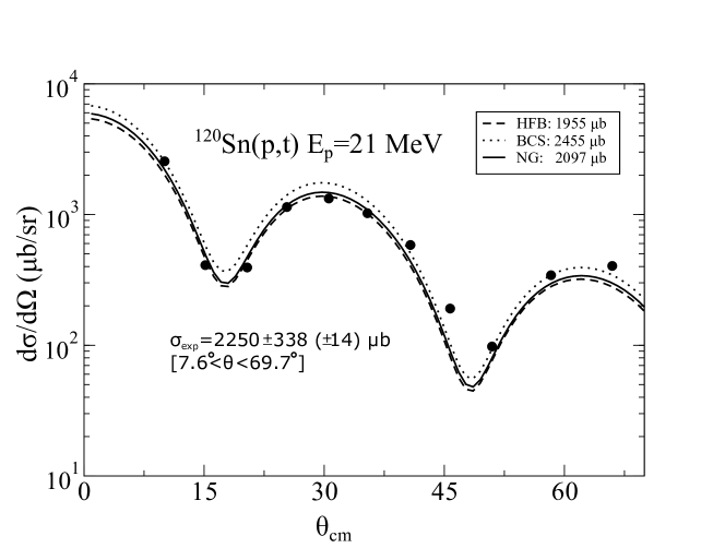
Figure 4: Absolute differential cross sections associated with the reaction ¹²⁰Sn(p,t)¹¹⁸Sn(gs) calculated making use of the BCS, HFB and renormalised NFT(NG) spectroscopic amplitudes (Table 2) and global optical parameters (Table 3), in comparison with the experimental findings (solid dots) Guazzoni .

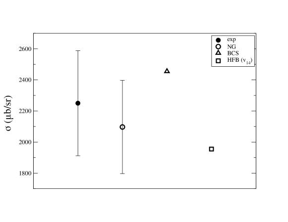
Figure 5: Integrated absolute cross sections associated with the reaction ¹²⁰Sn(p,t)¹¹⁸Sn(gs) (see caption to Fig. 4). The error ascribed to the NFT(NG) theoretical results stems from the uncertainties in the calculation of the two-neutron transfer spectroscopic amplitudes estimated from the variations the contribution of spin modes associated with different Skyrme interactions induce in the $B-$coefficients.

The results obtained from the solution of the Nambu-Gor’kov equation are collected in Table 1, together with those if HFB and BCS. The fragments carrying the largest fraction of the quasiparticle strength associated with each of the five valence orbitals of unperturbed energy $\epsilon_{a}$ are listed in order of increasing energy. For each fragment the value of the renormalised quasiparticle energy $\tilde{E}_{a(n)}$ and of the renormalized quasiparticle amplitudes $\tilde{u}_{a(n)},\tilde{v}_{a(n)}$ are provided, together with those of the renormalised single-particle energy $\tilde{\epsilon}_{a(n)}^{\prime}$ and of the renormalised pairing gap $\tilde{\Delta}_{a(n)}^{\prime}$.

The formalism outlined above has been used to compute the two–nucleon transfer spectroscopic amplitudes

$$\tilde{B}(a(n))=\sqrt{\frac{2j_{a}+1}{2}}\tilde{u}_{a(n)}\tilde{v}_{a(n)}=\sqrt{\frac{2j_{a}+1}{2}}\int^{\tilde{E}_{a(n)}+\tilde{\Gamma}_{a(n)}/2}_{\tilde{E}_{a(n)}-\tilde{\Gamma}_{a(n)}/2}\widetilde{S}_{a}(\omega)\textrm{d}\omega,$$ (33)

associated with the reaction ¹²⁰Sn$(p,t)^{118}$Sn$(gs)$ between two members of the Sn–ground state pairing rotational band. The corresponding results are shown in Table 1, in comparison to those corresponding to the HFB and BCS calcualtion. Making use of global optical potentials (Table 3), the absolute differential cross sections were calculated and are compared with the experimental findings in Fig. 4. Theory reproduces the experimental findings essentially at the 10% level (BCS 9.1%, HFB 13%, NFT (NG) 7%), well within experimental errors (see also Fig. 5). The stability of the theoretical results is apparent.

VII Discussion

The spectroscopic results reported in Table 1 testify to the important effects renormalisation of the single-particle states and of the pairing interaction have at the level of quasiparticles. In spite of this, all three approaches (NFT(NG),HFB, BCS), notwithstanding their large differences in terms of many-body facets, predict essentially equally correct absolute two-nucleon transfer cross sections, as testified by the results displayed in Figs. 4 and 5, where theory is compared to experiment,

It seems then fair to conclude that the quantity which controls the specific excitation of pairing rotational bands, namely the order parameter $\alpha_{0}$, in the sense of Cooper pair transfer amplitude (Sect. III), is essentially invariant, whether calculated within the framework of the simplest one-pole quasiparticle (BCS) approximation, or taking into account the variety of many-body renormalisation effects.

The emergence of a physical sum–rule is apparent (within this context see Broglia:72 , while for exact sum rules see Bayman:72 ; Lanford:77 ). Let us elaborate on this point.

Approximating

$$\tilde{u}_{a(n)}=\sqrt{N_{a(n)}}U_{a}\quad;\quad\tilde{v}_{a(n)}=\sqrt{N_{a(n)}}V_{a},$$ (34)

and

$$N_{a(n)}\approx Z_{a(n)}\approx Z_{\omega},\quad(\epsilon_{a}\approx\epsilon_{F})$$ (35)

one can write,

$$\alpha_{0}=\sum_{a,n}\frac{2j_{a}+1}{2}\tilde{u}_{a(n)}\tilde{v}_{a(n)}=\frac{N(0)}{Z_{\omega}}\int d\epsilon\frac{2j_{\epsilon}+1}{2}\tilde{u}_{\epsilon}\tilde{v}_{\epsilon},$$ (36)

where $N(0)/Z_{\omega}$ is the effective density of levels at the Fermi energy Schuck . With the help of Eq. (35) one obtains,

$$\alpha_{0}=\frac{N(0)}{Z_{\omega}}Z_{\omega}\int d\epsilon\frac{2j_{\epsilon}+1}{2}U_{\epsilon}V_{\epsilon}\approx\sum_{a}\frac{2j_{a}+1}{2}U_{a}V_{a}.$$ (37)

Using each term of the expressions (36) and (37) as weighting factors of the corresponding two–nucleon transfer formfactors, in keeping with the unified structure–reaction physical interpretation of $\alpha_{0}$ (Sect. III), and that (see Figs. 4 and 5) $|\sigma_{i}-\sigma_{exp}|/\sigma_{exp}$ is equal to 0.09, 0.13 and 0.07 ($i=$ BCS, HFB, NG), the relative errors of the associated two–nucleon transfer amplitudes $\alpha_{0}(\sim\sqrt{\sigma})$ are 4.5%, 6.5% and 3.5%. Within this context, it is of notice that the fact that the HFB result lies closer to the NG one than BCS does, is a simple consequence of NG being based on HFB.

Furthermore, because the matrix elements of $v_{14}$ for configurations based on the valence orbitals is essentially state independent together with the fact that $Z^{2}\approx 0.5$, setting $v_{ind}=0$, one expects for the renormalised (NFT(NG)) cross section a value $\approx 1000\mu b$ (0.5 $\times\sigma_{HFB}$), precluding the above accuracy. Consequently, at the basis of the validity of (36)–(37) and thus of the conservation of two–nucleon transfer amplitudes in going from BCS mean field to NFT(NG) many-body, medium renormalization representations, one also finds the central role played by the induced pairing interaction.

Chapter Appendix A. Off diagonal long range order (ODLRO)

The challenge solved by Schrieffer Schrieffer1964 in his contribution to BCS was that of writing, starting from Cooper single pair solution to pairing Cooper1956 , a many-particle wave function in which each electron moving close to the Fermi energy participated in the condensate. The main problem is that $N-$fixed many-body wave functions cannot have a definite phase. But if one uses a coherent state representation it is possible to describe a condensate with a definite phase. Schrieffer found a way to write down a coherent state of fermion pairs, namely (it is of notice that primed quantities are again being used , see footnote p. 3)

$$|BCS\rangle=\Pi_{\nu\rangle 0}(U_{\nu}+V_{\nu}a^{+}_{\nu}a^{+}_{\bar{\nu}})|0\rangle.$$ (A1)

Introducing the phasing

$$U_{\nu}=|U_{\nu}|=U^{\prime}_{\nu},\quad V_{\nu}=e^{-2i\phi}V^{\prime}_{\nu}(V^{\prime}_{\nu}\equiv|V_{\nu}|),$$ (A2)

one can write

$$|BCS(\phi)\rangle_{\cal K}=\Pi_{\nu\rangle 0}(U^{\prime}_{\nu}+V^{\prime}_{\nu}e^{-2i\phi}a^{+}_{\nu}a^{+}_{\bar{\nu}})|0\rangle$$ (A3)

$$=\Pi_{\nu\rangle 0}(U^{\prime}_{\nu}+V^{\prime}_{\nu}a^{\prime+}_{\nu}a^{\prime+}_{\bar{\nu}})|0\rangle=|BCS(0)\rangle_{\cal K^{\prime}},$$ (A4)

where $\cal K$ and $\cal K^{\prime}$ label the laboratory and the intrinsic (body-fixed BCS, deformed state in gauge space) frame of reference, while $a^{\prime+}_{\nu}={\cal G}(\phi)a^{+}_{\nu}{\cal G}^{-1}(\phi)=e^{-i\phi}$ $a^{+}_{\nu}(a^{\prime+}_{\bar{\nu}}$ $=e^{-i\phi}$ $a^{+}_{\bar{\nu}})$ is a creation operator referred to this intrinsic frame. The operator ${\cal G}(\phi)$ = exp$({-i{\hat{N}}\phi})$ induces a rotation of angle $\phi$ in gauge (two-dimensional) space (gauge transformation), with $\hat{N}$ being the number of particle operator. The states $|\nu\rangle$ and $|\bar{\nu}\rangle$, connected by the time-reversal operator, have the same energy (Kramers’ degeneracy).

A property of the above wave function, which has been given the name ”off-diagonal long-range order” (ODLRO) Yang1962 is of crucial importance regarding the physics at the basis of BCS condensation . This property can be extracted from the BCS wave function in a number of ways (see e.g. Ange )

To introduce the subject, let us start by writing down operators which create or annihilate pairs of fermions in the $\vec{r}$ representation, i.e. making use of
$\psi^{+}(\vec{r})=\langle\vec{r}|a^{+}_{\nu}|0\rangle$ and the Hermitian conjugate (see App. B). One can define the pair operator (see Fig. A1)

$$P^{+}(\vec{R})=\int d^{3}r\phi(\vec{r})\psi^{+}_{\nu}(\vec{R}+\vec{r}/2)\psi^{+}_{\bar{\nu}}(\vec{R}-\vec{r}/2),$$ (A5)

where $\phi(\vec{r})$ is the pair wave function. Thus $P^{+}(\vec{R})$ creates a spin singlet fermion pair where the particles are separated by the relative distance $\vec{r}$ and with centre of mass $\vec{R}$, i.e.

$$\vec{R}=\frac{\vec{r}_{1}+\vec{r}_{2}}{2}\quad,\quad\vec{r}=\vec{r}_{1}-\vec{r}_{2},$$ (A6)

and thus

$$\vec{r}_{1}=\vec{R}+\frac{\vec{r}}{2}\quad,\quad r_{2}=\vec{R}-\frac{\vec{r}}{2}.$$ (A7)

One can now define a density matrix

$$\rho(\vec{R}-\vec{R}^{\prime})=\langle P^{+}(\vec{R})P(\vec{R}^{\prime})\rangle,$$ (A8)

that is, a generalised particle (see Eq. (C1), App. C) density for pairs, the so called abnormal density, related to the two-particle density

$$\rho_{2}(\vec{r}_{1}\sigma_{1},\vec{r}_{2}\sigma_{2},\vec{r}_{3}\sigma_{3},\vec{r}_{4}\sigma_{4})=\langle\psi^{+}_{\nu}(\vec{r}_{1})\psi^{+}_{\bar{\nu}}(\vec{r}_{2})\psi^{+}_{\bar{\nu}^{\prime}}(\vec{r}_{3})\psi^{+}_{\nu^{\prime}}(\vec{r}_{4})\rangle.$$ (A9)

Making use of Eq. (A.1) one obtains,

$$\rho(\vec{R}-\vec{R}^{\prime})=\int d^{3}rd^{3}r\;^{\prime}\phi(\vec{r})\phi(\vec{r}\;^{\prime})$$

$$\times\rho_{2}(\vec{R}+\vec{r}/2,\sigma;\vec{R}-\vec{r}/2,-\sigma;\vec{R}\;^{\prime}-\vec{r}\;^{\prime}/2,-\sigma;R\;^{\prime}+\vec{r}\;^{\prime}/2,\sigma\;^{\prime}).$$ (A10)

The pair wave function $\phi(\vec{r})$ vanishes when the relative distance becomes larger than the correlation length $\xi$. Thus, $\rho$ is different from zero provided that $r(\equiv|\vec{r}_{1}-\vec{r}_{2}|)$ and $r^{\prime}(\equiv|\vec{r}_{1}\;^{\prime}-\vec{r}_{2}\;^{\prime}|)$, are smaller than $\xi$. But the pairs can be separated by any arbitrary distance. In other words, ${\rm lim}_{|\vec{R}-\vec{R}^{\prime}|\to\infty}\rho(\vec{R}-\vec{R}\;^{\prime})\neq 0$, that is ODLRO. And this is what the $|BCS\rangle$ state ensures, in keeping with the fact that it describes independent pair motion, in which all pairs are in the same state, i.e.

$$|BCS(\phi)\rangle_{\cal K}=\left(\Pi_{\nu>0}U^{\prime}_{\nu}\right)\{1+(\sum_{\nu>0}c^{\prime}_{\nu}e^{-2i\phi}a^{+}_{\nu}a^{+}_{\bar{\nu}}+$$

$$+\frac{1}{2!}(\sum_{\nu>0}c^{\prime}_{\nu}e^{-2i\phi}a^{+}_{\nu}a^{+}_{\bar{\nu}})^{2}+\frac{1}{3!}(\sum_{\nu>0}c^{\prime}_{\nu}e^{-2i\phi}a^{+}_{\nu}a^{+}_{\bar{\nu}})^{3}+...\}$$ (A11)

where

$$c^{\prime}_{\nu}=\frac{V^{\prime}_{\nu}}{U^{\prime}_{\nu}}.$$ (A12)

This is the mean field solution of the pairing Hamiltonian. In other words, the ground state of the mean-field pairing Hamiltonian

$$H_{MF}=U+H_{11},$$ (A13)

where

$$U=2\sum_{\nu>0}(\epsilon_{\nu}-\lambda)V^{2}_{\nu}-\frac{\Delta^{2}}{G},$$ (A14)

and

$$H_{11}=\sum_{\nu}E_{\nu}\;\alpha^{+}_{\nu}\alpha_{\nu}.$$ (A15)

Gauge symmetry restoration is obtained by taking into account the interaction

$$H^{\prime\prime}_{p}=\frac{G}{4}\left(\sum_{\nu>0}(\Gamma^{+}_{\nu}-\Gamma_{\nu})\right)^{2},$$ (A16)

acting among the quasiparticles where $\Gamma^{+}_{\nu}=\alpha^{+}_{\nu}\alpha^{+}_{\bar{\nu}}$. In fact, it can be shown that

$$[H_{MF}+H^{\prime\prime}_{p},\hat{N}]=0,$$ (A17)

$\hat{N}$ being the number of particle operator. Diagonalising Eq. (A16) in QRPA, i.e.

$$[H_{MF}+H^{\prime\prime}_{p},\Gamma^{\prime\prime+}_{n}]=W^{\prime\prime}_{n}\Gamma^{+}_{n},$$ (A18)

where

$$\Gamma^{\prime\prime+}_{n}=\sum_{\nu>0}(a_{n\nu}\Gamma^{+}_{\nu}+b_{n\nu}\Gamma_{\nu}),$$ (A19)

the associated dispersion relation reads

$$\sum_{\nu>0}\frac{2E_{\nu}}{(2E_{\nu})^{2}-(W^{\prime\prime}_{n})^{2}}=\frac{1}{G},$$ (A20)

while

$$a_{n\nu}=\frac{\Lambda^{\prime\prime}_{n}}{2E_{\nu}-W^{\prime\prime}_{n}}\quad,\quad b_{n\nu}=\frac{\Lambda^{\prime\prime}_{n}}{2E_{\nu}+W^{\prime\prime}_{n}},$$ (A21)

with

$$\Lambda^{\prime\prime}_{n}=\frac{1}{2}\left(\sum_{\nu>0}\frac{2E_{\nu}W^{\prime\prime}_{n}}{((2E_{\nu})^{2}-(W^{\prime\prime}_{n})^{2})^{2}}\right)^{-1/2}.$$ (A22)

The lowest - most ”collective” - root of Eq. (A20) has $W^{\prime\prime}_{1}=0$ (BCS gap equation), the associated eigenstate being

$$|1^{\prime\prime}\rangle=\Gamma^{\prime\prime+}_{1}|0\rangle=\Lambda^{\prime\prime}_{1}\sum_{\nu>0}\frac{1}{2E_{\nu}}(\Gamma^{+}_{\nu}+\Gamma_{\nu})|0^{\prime\prime}\rangle.$$ (A23)

In keeping with the fact that, in QRPA, the number operator reads

$$\tilde{N}=\Delta\sum_{\nu>0}\frac{1}{E_{\nu}}(\Gamma^{+}_{\nu}+\Gamma_{\nu})+N_{0},$$ (A24)

one can write

$$|1^{\prime\prime}\rangle=\Gamma^{\prime\prime+}_{1}|0\rangle=\frac{\Lambda^{\prime\prime}_{1}}{2\Delta}(\tilde{N}-N_{0})|0^{\prime\prime}\rangle.$$ (A25)

A finite rotation in gauge space can be generated by a series of infinitesimal operations induced by the operator ${\cal G}(\phi)=$ exp $(-i\hat{N}\phi)$, i.e.

$${\cal G}(\delta\phi)\approx 1-i{\hat{N}}\delta\phi.$$ (A26)

Within this context, $i({\cal G}(\delta\phi)-({\cal G}(0)-iN_{0}\delta\phi))=(\hat{N}-N_{0})\delta\phi$, where $\delta\phi=\Lambda^{\prime\prime}_{1}/(2\Delta)$ (Eq. (A25 ). Because $\Lambda^{\prime\prime}_{1}$ diverges as $W^{\prime\prime}_{1}\to 0$, $(\hat{N}-N_{0})|{\tilde{0}^{\prime\prime}}\rangle\approx(\tilde{N}-N_{0})|{\tilde{0}^{\prime\prime}}\rangle\to 0$, in keeping with Eq. (A17).

Divergence in gauge angle implies that $\phi$ can have any value in the range $0-2\pi$. Consequently the system will be in a given member of a pairing rotational band, e.g.

$$|\tilde{N}\rangle\sim\int d\phi e^{i(N/2)\phi}|BCS(\phi)\rangle_{\cal K}\sim O^{N/2}|0\rangle,$$ (A27)

where

$$O=\sum_{\nu>0}c^{\prime}_{\nu}a^{+}_{\nu}a^{+}_{\bar{\nu}}.$$ (A28)

One now rewrites $O$ as

$$O=\int d^{3}r_{1}d^{3}r_{2}\chi(r_{1},r_{2})\psi^{+}_{\uparrow}(\vec{r}_{1})\psi^{+}_{\downarrow}(\vec{r}_{2})=\sum_{k}\chi(\vec{k})a^{+}_{\vec{k}\uparrow}a^{+}_{\vec{k}\downarrow},$$ (A29)

where $\chi(\vec{k})=V^{\prime}_{k}/U^{\prime}_{k}$, and define the normalised $N-$particle state as

$$|N\rangle={\cal N}_{N}O^{N/2}|0\rangle$$ (A30)

and the one-particle density matrix according to

$$\phi(\vec{r}_{1},\vec{r}_{1}\;^{\prime})\equiv\langle N|\psi^{+}_{\uparrow}(\vec{r}_{1})\psi_{\uparrow}(\vec{r}_{1}\;^{\prime})|N\rangle=\langle N|\psi^{+}_{\uparrow}(\vec{r}_{1})\psi_{\downarrow}(\vec{r}_{1}\;^{\prime})|N\rangle.$$ (A31)

Making use of $\psi|0\rangle=0$ and of the commutator

$$[\psi_{\uparrow}(\vec{r}_{1}),O^{N/2}]=\frac{N}{2}\int d^{3}r_{2}\chi(\vec{r}_{1},\vec{r}_{2})\psi^{+}_{\uparrow}(\vec{r}_{2})O^{(N-2)/2},$$ (A32)

one can write

$$\phi(\vec{r}_{1},\vec{r}_{1}\;^{\prime})=\int d^{3}r_{2}\tilde{\chi}(\vec{r}_{1}\;^{\prime},\vec{r}_{2})\langle N|\psi^{+}_{\uparrow}(\vec{r}_{1})\psi^{+}_{\downarrow}(\vec{r}_{2})|N-2\rangle$$ (A33)

where

$$\tilde{\chi}(\vec{r}_{1},\vec{r}_{2})=(N/2){\cal N}_{N}{\cal N}^{-1}_{N-2}\chi(\vec{r}_{1},\vec{r}_{2}).$$ (A34)

The matrix element in Eq. (A33) is closely related with Gorkov’s amplitude for two fermions at $\vec{r}_{1}$ and $\vec{r}_{2}$ to belong to a Cooper pair, i.e.

$$F^{>}(\vec{r}_{1},\vec{r}_{2})=-i\langle N-2|\psi_{\uparrow}(\vec{r}_{1})\psi_{\downarrow}(\vec{r}_{2})|N\rangle,$$ (A35)

its complex conjugate being

$$F^{>}(\vec{r}_{1},\vec{r}_{2})^{*}=i\langle N|\psi^{+}_{\downarrow}(\vec{r}_{2})\psi^{+}_{\uparrow}(\vec{r}_{1})|N-2\rangle$$

$$=-i\langle N|\psi^{+}_{\uparrow}(\vec{r}_{1})\psi^{+}_{\downarrow}(\vec{r}_{2})|N-2>.$$ (A36)

Thus, Eq. (A33) can be written as

$$\phi(\vec{r}_{1},\vec{r}_{1}\;^{\prime})=i\int d^{3}r_{2}\;\tilde{\chi}(\vec{r}_{1}\;^{\prime},\vec{r}_{2})F^{\rangle}(\vec{r}_{1},\vec{r}_{2})^{*}.$$ (A37)

Let us now consider the two-particle matrix density

$$\phi(\vec{r}_{1},\vec{r}_{2};\vec{r}_{3},\vec{r}_{4})\equiv\langle N|\psi^{+}_{\uparrow}(\vec{r}_{1})\psi^{+}_{\downarrow}(\vec{r}_{2})\psi_{\downarrow}(\vec{r}_{4})\psi_{\uparrow}(\vec{r}_{3})|N\rangle$$

$$=\phi(\vec{r}_{1},\vec{r}_{3})\phi(\vec{r}_{2},\vec{r}_{4})+F^{>}(\vec{r}_{1},\vec{r}_{2})^{*}F^{>}(\vec{r}_{3},\vec{r}_{4}),$$ (A38)

equivalent to

$$\langle N|\psi_{\uparrow}^{+}(\vec{r}_{1})\psi^{+}_{\downarrow}(\vec{r}_{2})\psi_{\downarrow}(\vec{r}_{4})\psi_{\uparrow}(\vec{r}_{3})|N\rangle$$

$$=\langle N|\psi_{\uparrow}^{+}(\vec{r}_{1})\psi_{\uparrow}(\vec{r}_{3})|N\rangle\langle N|\psi_{\downarrow}^{+}(\vec{r}_{2})\psi_{\downarrow}(\vec{r}_{4})|N\rangle$$

$$+\langle N|\psi_{\uparrow}^{+}(\vec{r}_{1})\psi^{+}_{\downarrow}(\vec{r}_{2})|N-2\rangle\langle N-2|\psi_{\downarrow}(\vec{r}_{3})\psi_{\uparrow}(\vec{r}_{4})|N\rangle.$$ (A39)

The wave function (A38) thus leads to a two-particle density matrix fulfilling

$${\rm lim}_{\vec{r}_{1},\vec{r}_{2}\to\infty;\vec{r}_{3},\vec{r}_{4}\to-\infty}\phi(\vec{r}_{1},\vec{r}_{2};\vec{r}_{3},\vec{r}_{4})\quad\quad(r_{12},r_{34}\langle\xi),$$

$$=lim_{\vec{r}_{1}\vec{r}_{2}\to\infty}[F^{>}(\vec{r}_{1},\vec{r}_{2})^{*}]\times[{\rm lim}_{\vec{r}_{3}\vec{r}_{4}\to-\infty}F^{>}(\vec{r}_{3},\vec{r}_{4})]\neq 0,$$ (A40)

property known as ODLRO.

Within the nuclear embodiment, the wave function (A30) describes the properties of a member of a pairing rotation band. For example the ground state of one of the superfluid Sn-isotopes, in particular ¹²⁰Sn(gs). In a reaction like ¹²⁰Sn + ¹¹⁸Sn $\to$ ¹¹⁸Sn(gs) + ¹²⁰Sn(gs), at energies where the distance of closest approach is $2R_{o}+a\approx$ 13 fm ($E_{CM}\approx$ 270 MeV) a number of the effects discussed above can materialise (Fig. A2). In the tunnelling of a Cooper pair from a superfluid nucleus to the other, each partner can be in a different nucleus, but still correlated. This is in keeping who the fact that the correlation length arising from the empirical pairing gap ($\Delta\approx 1.4$ MeV), resulting from the summed contribution of the bare and induced pairing interaction is $\xi=\hbar v_{F}/\pi\Delta\approx$ 12 fm.

Let us go back to the QRPA (harmonic) diagonalization of $H=H_{MF}+H_{p}^{\prime\prime}$. One can rewrite $H$ as the oscillator Brink2005 ,

$$H=\frac{p^{2}}{2D^{\prime\prime}_{1}}+\frac{1}{2}D^{\prime\prime}_{1}\omega^{\prime\prime}_{1}q^{2}$$ (A41)

and identify the momentum with the number operators, the coordinate with the gauge angle and the frequency with the QRPA energy,

$$p=\hbar(\tilde{N}-N_{0}),\quad q=\phi,\quad\hbar\omega^{\prime\prime}_{1}=W_{1}^{\prime\prime}.$$ (A42)

The phonon creation operator for the oscillator is

$$\Gamma^{\prime\prime+}_{1}=\sqrt{\frac{\hbar^{2}}{2D^{\prime\prime}W_{1}^{\prime\prime}}}(\tilde{N}-N_{0})+i\phi\sqrt{\frac{D_{1}^{\prime\prime}W_{1}^{\prime\prime}}{2\hbar^{2}}}.$$ (A43)

Comparing the coefficient of $(\tilde{N}-N_{o})$ in Eq. (A25) and (A43), and noting that the coefficient of $\phi$ in Eq. (A43) vanishes in the limit $W^{\prime\prime}_{1}\to 0$, we get an expression for the mass parameter

$$\frac{\hbar^{2}}{2D^{\prime\prime}_{1}W^{\prime\prime}_{1}}=\left(\frac{\Lambda^{\prime\prime}_{1}}{2\Delta}\right)^{2},$$ (A44)

or

$$\frac{D^{\prime\prime}_{1}}{\hbar^{2}}=\frac{4\Delta^{2}}{2W^{\prime\prime}_{1}\Lambda^{\prime\prime 2}_{1}}.$$ (A45)

Making use of Eq. (A22) one obtains

$$\frac{1}{W^{\prime\prime}_{1}\Lambda_{1}^{\prime\prime 2}}=4\sum_{\nu>0}\frac{2E_{\nu}}{((2E_{\nu})^{2}-(W^{\prime\prime}_{1})^{2})^{2}}.$$ (A46)

In the limit $W^{\prime\prime}_{1}\to 0$ this relation becomes

$$\frac{1}{W^{\prime\prime}_{1}\Lambda^{\prime\prime 2}_{1}}=\sum_{\nu>0}\frac{1}{2E^{3}_{\nu}},$$ (A47)

and the mass parameter can be written as,

$$\frac{D^{\prime\prime}_{1}}{\hbar^{2}}=\sum_{\nu>0}\frac{\Delta^{2}}{E^{3}_{\nu}},$$ (A48)

emergent property of generalised rigidity in gauge space for a nucleus whose mean field solution violates gauge invariance.

Making use of Eq. (A48), and of the fact that $\lambda=\partial H/\partial N$, the energy of the members of a pairing rotational band can be written as

$$E_{N}=\lambda N+\frac{\hbar^{2}}{2{\cal J}}N^{2},$$ (A49)

where

$$\frac{\cal{J}}{\hbar^{2}}=\frac{D^{\prime\prime}_{1}}{\hbar^{2}}=\sum_{\nu>0}\frac{4U_{\nu}^{2}V_{\nu}^{2}}{E_{\nu}}=2\sum_{\nu>0}\frac{\langle\nu\bar{\nu}|\hat{N}|BCS\rangle^{2}}{2E_{\nu}},$$ (A50)

is the cranking formula of the moment of inertia rotations in gauge space. In deriving the above expression use was made of the BCS relation $2U_{\nu}V_{\nu}=\Delta/E_{\nu}$. Pairing rotations can be viewed as the Goldstone–mode, or better the Anderson–Goldstone–Nambu mode Bes1966 ; Hinohara2016 ; Broglia2000 ; Lopez:13 in gauge space, approaching the $E=0$ limit linear with $N$. This is in keeping with the fact that such behavior is only expected in the laboratory system, where it can be measured. In other words, summing to the BCS energy $U$ the Coriolis force $\lambda N$ in gauge space felt by the condensate in the intrinsic system.

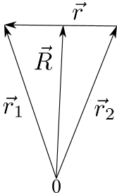
Figure A6: Coordinates used to define the pair operator $P^{+}(\vec{R})$.

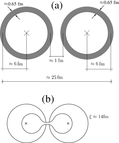
Figure A7: (a) Schematic representation of two Sn nuclei at a distance of closest approach of $\approx 13$ fm. (b) Single Cooper pair in which each nucleon is in a different nucleus.

Chapter Appendix B. Useful definitions

Making use of the wave function $u_{\nu}(\vec{r},\sigma)$, position and spin representation of the ket $|\nu\rangle$ describing the single-particle motion of a nucleon in the state $\nu$,

$$u_{\nu}(\vec{r},\sigma)=\langle\vec{r},\sigma|\nu\rangle$$ (B1)

one can define the field operator

$$\psi(\vec{r},\sigma)=\sum_{\nu}\langle\vec{r},\sigma|\nu\rangle a_{\nu}=\sum_{\nu}u_{\nu}(\vec{r},\sigma)a_{\nu},$$ (B2)

$a_{\nu}$ being the annihilation operator of a fermion in state $\nu$. Thus, $\psi(\vec{r},\sigma)$ is an operator in the occupation-number space and also a function of position and spin, while

$$\psi^{+}(\vec{r},\sigma)=\sum_{\nu}u_{\nu}^{*}(\vec{r},\sigma)a^{+}_{\nu}$$ (B3)

is its hermitian conjugate, $a^{+}_{\nu}$ being the creation operator of a fermion in state $\nu$, i.e. $|\nu\rangle=a^{+}_{\nu}|0\rangle$, $|0\rangle$ being the vacuum state.

A one-particle operator, e.g. the one-particle potential can be written as,

$$U=\sum_{\nu,\nu^{\prime}}\langle\nu|V|\nu^{\prime}\rangle a^{+}_{\nu}a_{\nu^{\prime}},$$ (B4)

where

$$\langle\nu|U|\nu^{\prime}\rangle=\sum_{\sigma,\sigma^{\prime}}\int d^{3}r\langle\nu|\vec{r},\sigma\rangle\langle\vec{r},\sigma|U|\vec{r},\sigma\rangle\langle\vec{r},\sigma^{\prime}|\nu^{\prime}\rangle$$

$$=\sum_{\sigma,\sigma^{\prime}}\int d^{3}r\;u^{*}_{\nu}(\vec{r},\sigma)V_{\sigma,\sigma^{\prime}}(\vec{r})u_{\nu^{\prime}}(\vec{r},\sigma^{\prime}).$$ (B5)

Thus,

$$U=\sum_{\sigma,\sigma^{\prime}}\int d^{3}r\sum_{\nu,\nu^{\prime}}u^{*}_{\nu}(\vec{r},\sigma)U_{\sigma,\sigma^{\prime}}(\vec{r})u_{\nu^{\prime}}(\vec{r},\sigma^{\prime})a^{+}_{\nu}a_{\nu^{\prime}}.$$ (B6)

Making use of Eq. (B2) and (B3) one can write,

$$U=\sum_{\sigma,\sigma^{\prime}}\int d^{3}\psi^{+}(\vec{r},\sigma)U_{\sigma,\sigma}\psi(\vec{r},\sigma^{\prime}).$$ (B7)

Let us consider now the two-body interaction

$$v=-\frac{1}{2}\sum_{\nu_{1}\nu_{2}\nu_{1}^{\prime}\nu_{2}^{\prime}}v_{\nu_{1}\nu_{2},\nu_{1}^{\prime}\nu_{2}^{\prime}}a^{+}_{\nu_{2}}a^{+}_{\nu_{1}}a_{\nu_{1}^{\prime}}a_{\nu^{\prime}_{2}},$$ (B8)

where

$$v_{\nu_{2}\nu_{1},\nu_{1}^{\prime}\nu_{2}^{\prime}}=\langle\nu_{2}\nu_{1}|v|\nu_{1}^{\prime}\nu_{2}^{\prime}\rangle=\int d^{3}r_{1}d^{3}r_{2}\sum_{\sigma_{1},\sigma_{2},\sigma_{1}^{\prime}\sigma_{2}^{\prime}}\langle\nu_{2}|\vec{r}_{2},\sigma_{2}\rangle\langle\nu_{1}|\vec{r}_{1},\sigma_{1}\rangle$$

$$\times\langle\vec{r}_{2},\sigma_{2};\vec{r}_{1},\sigma_{1}|v|\vec{r}_{1},\sigma^{\prime}_{1};\vec{r}_{2},\sigma_{2}\rangle\langle\vec{r}_{1},\sigma^{\prime}_{1}|\nu^{\prime}_{1}\rangle\langle\vec{r}_{2},\sigma^{\prime}_{2}|\nu^{\prime}_{2}\rangle$$

$$=\sum_{\sigma_{1},\sigma_{2},\sigma^{\prime}_{1},\sigma^{\prime}_{2}}\int d^{3}r_{1}d^{3}r_{2}u^{*}_{\nu_{2}}(\vec{r}_{2},\sigma_{2})u^{*}_{\nu_{1}}(\vec{r}_{1},\sigma_{1})v_{\sigma_{2}\sigma_{1},\sigma^{\prime}_{1}\sigma^{\prime}_{2}}(\vec{r}_{1},\vec{r}_{2})$$

$$\times u_{\nu^{\prime}_{1}}(\vec{r}_{1},\sigma^{\prime}_{1})u_{\nu^{\prime}_{2}}(\vec{r}_{2}^{\prime}.\sigma^{\prime}_{2}).$$ (B9)

Thus

$$v=-\frac{1}{2}\sum_{\sigma_{1},\sigma_{2},\sigma^{\prime}_{1},\sigma^{\prime}_{2}}\int d^{3}r_{1}d^{3}r_{2}$$

$$\sum_{\nu_{1},\nu_{2},\nu^{\prime}_{1},\nu^{\prime}_{2}}u^{*}_{\nu_{2}}(\vec{r}_{2},\sigma_{2})u^{*}_{\nu_{1}}(\vec{r}_{1},\sigma_{1})v_{\sigma_{2}\sigma_{1},\sigma^{\prime}_{1}\sigma^{\prime}_{2}}(\vec{r}_{1},\vec{r}_{2})$$

$$\times u_{\nu^{\prime}_{1}}(\vec{r}_{1}\;^{\prime},\sigma^{\prime}_{1})u_{\nu^{\prime}_{2}}(\vec{r}_{2}\;^{\prime},\sigma^{\prime}_{2})a^{+}_{\nu_{2}}a^{+}_{\nu_{1}}a^{\prime}_{\nu_{1}}a_{\nu_{2}}^{\prime}$$

$$=\frac{1}{2}\sum_{\sigma_{1},\sigma_{2},\sigma_{1}^{\prime},\sigma_{2}^{\prime}}\int d^{3}r_{1}d^{3}r_{2}\psi^{+}(\vec{r}_{2},\sigma_{2})\psi^{+}(\vec{r}_{1},\sigma_{1})$$

$$\times v_{\sigma_{2}\sigma_{1},\sigma_{1}^{\prime}\sigma_{2}^{\prime}}(\vec{r}_{1},\vec{r}_{2})\psi(\vec{r}_{2},\sigma_{2}^{\prime})\psi(\vec{r}_{1},\sigma_{1}^{\prime}).$$ (B10)

Chapter Appendix C. One- and two-body Dirac matrices

Short before the appearance of the BCS papers Bardeenetal1957a ; Bardeenetal1957b , the result of a study concerning the nature of the order parameter of a boson superfluid, such as ⁴He below 2.17 K, was published Penrose . In this reference it was argued that the Bose condensation that is supposed to be responsible for superfluidity should manifest itself in the off-diagonal elements of the one-particle density matrix

$$\rho(\vec{r},\vec{r}\;^{\prime})=\langle\phi^{+}(\vec{r}\;^{\prime})\phi(\vec{r})\rangle,$$ (C1)

where $\phi^{+}(\phi)$ are boson creation (annihilation) operators, the expectation value being taken in some statistical ensemble of states. This Dirac density matrix is Hermitian, its trace giving the total number of bosons $N$. In the normal state its eigenvalues are all at most of order unity, but in the superfluid state there is a macroscopic eigenvalue $n_{o}$, much larger than one. In the case of superfluid helium (⁴He) $n_{o}/N$ seems to be of the order of 10%, $N$ being the total number of atoms. In other words when $\vec{r}$ and $\vec{r}\;^{\prime}$ are far apart $\rho(\vec{r},\vec{r}\;^{\prime})$ must tend to $n_{o}/N$ in the superfluid state. This is a feature which is very different from that of a solid e.g. argon at low temperature, and is due to the high zero point motion of the light helium atoms, and the weak interaction between them. In the case of solid argon, the removal of one particle from its equilibrium position and transport to a distant point creates a vacancy-interstitial pair, the energy barrier associated with such process makes the amplitude of off-diagonal elements of the one-particle density matrix to fall off exponentially with the separation of the two coordinates.

In the case of fermions such as electrons or ³He atoms, the one-particle density matrix cannot have a macroscopic eigenvalue, since its eigenvalues lie in the range [0,1], but the two-particle density can Yang1962 . The two-particle Dirac density matrix has the form,

$$\Gamma(\vec{R}^{\prime},\vec{r}\;^{\prime};\vec{R},\vec{r})=\langle\psi^{+}(\vec{R}\;^{\prime}+\frac{\vec{r}\;^{\prime}}{2})\psi^{+}(\vec{R}^{\prime}-\frac{\vec{r}\;^{\prime}}{2})\psi(\vec{R}-\frac{\vec{r}}{2})\psi(\vec{R}+\frac{\vec{r}}{2}),$$ (C2)

where, for simplicity, the spin variables for the fermion creation and annihilation operators $\psi^{+},\psi$ have been suppressed. Disregarding, again for simplicity, crystal structure and disorder of the lattice, electrons move in a translational invariant environment. In that case ,the eigenvectors of the matrix depend on the center of mass coordinates only through factors of type $exp(i\vec{K}\cdot\vec{R}$). In the BCS ground state,

$$\Gamma=\delta(K^{\prime},0)\delta(K,0)U_{k^{\prime}}V_{k^{\prime}}U_{k}V_{k}.$$ (C3)

In configuration space the eigenvector corresponding to the macroscopic eigenvalue is the Fourier transform of this factor, so that the order parameter of the ground state is constant in $\vec{R}$ and $\vec{R}\;^{\prime}$, and is spread out in its internal coordinates $\vec{r}\;$ and $\vec{r}\;^{\prime}\,$ by an amount which depends on how strongly peaked the coherence fact is about the Fermi surface. This dependence on $\vec{r}$ gives the wave function of the Cooper pair.

In other words, and in keeping with the fact that, according to Wick’s theorem,

$$\Gamma(\vec{r}_{1},\vec{r}_{2};\vec{r}_{1}\;^{\prime},\vec{r}_{2}\;^{\prime})=\langle\psi^{+}(\vec{r}_{2}\;^{\prime})\psi^{+}(\vec{r}_{1}\;^{\prime})\psi(\vec{r}_{1})\psi(\vec{r}_{2})\rangle=$$

$$\rho(\vec{r}_{2},\vec{r}_{1}\;^{\prime})\rho(\vec{r}_{2},\vec{r}_{2}\;^{\prime})-\rho(\vec{r}_{1},\vec{r}_{2}\;^{\prime})\rho(\vec{r}_{2},\vec{r}_{1}\;^{\prime})+\chi^{*}(\vec{r}_{2}\;^{\prime},\vec{r}_{1}\;^{\prime})\chi(\vec{r}_{2},\vec{r}_{1}),$$ (C4)

where $\chi^{*}(\vec{r}_{1},\vec{r}_{2})=\langle\psi(\vec{r}_{1})\psi(\vec{r}_{2})\rangle,$ the eigenvector of $\Gamma$ being the (pairing) function $\chi$. That is ,

$$\int\int\Gamma(\vec{r}_{1},\vec{r}_{2};\vec{r}_{1}^{\prime},\vec{r}_{2})\chi(\vec{r}_{1}\;^{\prime}\vec{r}_{2}\;^{\prime})d^{3}r_{1}^{\prime}d^{3}r_{2}^{\prime}\approx n_{0}\chi(\vec{r}_{1},\vec{r}_{2}),$$ (C5)

where the eigenvalue, namely the pair density, is large, and is related to the large overlap of Cooper pairs at the basis of BCS theory. Within this context, the coherence length of a metallic superconductor being of the order of $10^{4}\AA$, implies that there are of the order of $10^{11}$ the electrons within a coherence volume, in keeping with the fact an electron typically occupies a volume $\approx(2\AA)^{3}$ (Wigner-Seitz cell).

In a neutron superfluid nucleus like e.g. ¹²⁰Sn, close to 15% of all nucleons participate in the condensate, the number of Cooper pairs being of the order of 5-6.

Chapter Appendix D. NFT vacuum polarization

The role zero point fluctuations play in the nuclear ground state, i.e. in the NFT vacuum can be clarified by relating it to the polarisation of the QED vacuum. Let us briefly dwell on the ”reality” of such phenomenon by recalling the fact that to the question of Rabi of whether the polarisation of the QED vacuum could be measured Pais - in particular the change in charge density felt by the electrons of an atom, e.g. the electron of a hydrogen atom, due to virtual creation and annihilation of electron-positron pairs - Lamb gave a quantitative answer, both experimentally and theoretically Lamb ; Kroll . The corresponding correction (Lamb shift) implies that the $2s_{1/2}$ level lies higher than the $2p_{1/2}$ level by about 1000 megacyles/s as experimentally observed.

In connection with the discussion of Feynman of vacuum polarisation, where a field produces a pair, the subsequent pair annihilation producing a new field, namely a close loop, he implemented in his space–time trajectories Wheeler’s idea of electrons going backwards in time (positrons). Such trajectories would be like an $\mathbf{N}$ in time, that is electrons which would back up for a while, and go forward again. Being connected with a minus sign, these processes are associated with Pauli principle in the self–energy of electrons (see Fig. 1,I(c)). The divergences affecting such calculations could be renormalised by first computing the self-energy diagram in second order and finding the answer which is finite, but contains a cut-off to avoid a logarithmic divergence. Expressing the result in terms of the experimental mass, one can take the limit (cut-off $\to\infty$) which now exists. Concerning radiative corrections to scattering, in particular that associated with the process in which the potential creates an electron-positron pair which then reannihilates, emitting a quantum which scatters the electron, the renormalisation procedure should be applied to the electric charge, introducing the observed one (Bethe and Pauli, see Bethe ).

In the nuclear case, for example Skyrme effective interactions give rise to particle-vibration coupling vertices which, because of the contact character of these interactions may lead to divergent zero point energies, unless a cut-off is introduced. The Gogny force being finite range does not display such problems. Nonetheless, the associated results concerning zero point energies may not be very stable and/or accurate carrying out a complete summation over both collective and non collective contributions. In this case one can eliminate such a problem by going to higher orders in the oyster diagrams (see Fig. 1(I)(a)). The fermion exchange between two of these diagrams (Pauli principle) essentially eliminates all of the non-collective contributions, leading to accurate results.

An economic and quite reliable method to achieve a similar result, is that of using empirical renormalisation. That is, to calculate the lowest order diagrams but introducing, in the intermediate states, the dressed physical (empirical) states (11Be ; Mattuck ; see also Bes1977 ).

Chapter Appendix E. State dependent effective mass and mean field potential

The bare mass of a nucleon in the nucleus is not a quantity that can be measured. This is because a nucleon in the nucleus is subject to a mean field which is both non-local in space as well as in time.

The first component arises already at the level of Hartree-Fock, and is directly related to the Hartree exchange potential, assuming velocity independent interactions. This non locality can be taken care of, in most situations, in terms of an effective mass, the $k$-mass, its average value being $m_{k}\approx 0.7m$, where $m$ is the bare mass. The quantity $m_{k}$ is intimately related to the so called Perey-Buck potential, namely the energy dependent term in the strength $V=V_{0}+0.4E$ of the real part of the optical potential needed to describe nucleon-nucleus elastic scattering experiments at bombarding energies of tens of MeV, where $E=|\epsilon_{k}-\epsilon_{F}|(\epsilon_{k}=\hbar^{2}k^{2}/2m)$. One can obtain essentially the same results by solving the elastic scattering single-particle Schrödinger equation making use of an energy independent potential of strength $V\approx\left(m/m_{k}\right)V_{0}=1.4V_{0}$ and of an effective mass $m_{k}=\left(m(1+(m/(\hbar^{2}k)dV/dk\right)^{-1}$ (within this context see Fig. 2.14 in Mahaux ). Similar results and protocol are obtained and can be used to describe deep hole states.

In other words, the concept of a single, mean field potential is a somewhat illusory one. This is even more so in keeping with the fact that there is not a single $k-$mass, but a state dependent one equal to the expectation value of the quantity in parenthesis, where $V$ is now the sum of the direct and exchange potential, calculated making use of the corresponding single-particle wave functions Bernard .

Retardation effects arise from the coupling of single-particles with collective vibrations (Fig. 1(I)). They lead, for states close to the Fermi energy, to the state-dependent $\omega-$mass ($m_{\omega}=m(1+\lambda),Z_{\omega}=m/m_{\omega}$), and to fragmentation, effects which can hardly be parameterised in terms of an average mean field potential.

In other words, the above effects are at the basis of the dynamical shell model. While one can, within this context, accurately calculate the single-particle properties ($\tilde{\epsilon}_{a(n)},Z_{a(n)},N_{a(n)})$ in simple and economic ways,e.g. renormalized NFT, the situation is much more complex concerning the absolute value of the Fermi energy.

Chapter Appendix F. Correlation length, correlation energy, generalised quantity parameter

The correlation length is defined as (Schrieffer1964 , p.18)

$$\xi=\frac{\hbar v_{F}}{\pi\Delta},$$ (F1)

while the condensation energy i.e. the difference between the ground state energy of the normal $(N)$ and superfluid $(S)$ phases is (Schrieffer1964 , eq. (2-35))

$$E_{cond}=W_{N}-W_{S}=\frac{1}{2}N(0)\Delta^{2}.$$ (F2)

In the above equations $v_{F}$ is the Fermi velocity , $\Delta$ the pairing gap, and $N(0)$ the density of levels at the Fermi energy for one spin orientation. The correlation energy $E_{corr}$ introduced in Bohr1975 (Eq. (6-618)) has the opposite sign to (F2). Concerning the density of levels of the corresponding reference, a spectrum of equally spaced levels, each of them displaying two-fold Kramers’ degeneracy was used, typical of quadrupole deformed nuclei (Nilsson model). Calling $d$ the spacing between them ($d\approx$ 0.4-0.5 MeV), the density of levels for both spin orientation is $2/d$, while $N(0)=1/d$. Thus, $E_{corr}=-\Delta^{2}/2d$ coincides in absolute value with (F2), as expected.

Making use of the empirical values for the density of levels of both spin orientations, namely $a=N/8$ MeV^-1 (Bortgdr , eq. (7.16)) one obtains for ${}^{120}_{50}$Sn₇₀, $N(0)\approx$ 4 MeV^-1. It is of notice that for this nucleus the empirical value of the pairing gap is $\Delta\approx 1.45$ MeV. The associated correlation length amounts to $\xi\approx 12$ fm. That associated with $\Delta_{ind}=(1/2)\Delta$ being of course 24 fm, value appearing in Eq. (11). Thus $E_{corr}\approx-$ 5 MeV, while the value associated with $\Delta_{ind}(\approx 0.8$ MeV) is -1.3 MeV. Making use of the above values, the generalised quantality parameter is,

$$q_{\xi}=\frac{\hbar^{2}}{2m\xi^{2}}\frac{1}{|E_{corr}|}=0.03\;(\xi=12\;{\rm fm},E_{corr}=-5\;{\rm MeV}),$$ (F3)

and testifies to a strong correlation between the partners of the Cooper pair.

Chapter Appendix G. Induced pairing interaction

The exchange of collective vibrations between nucleons moving in time reversal states give rise to an induced, medium polarization, pairing interaction. In the quasiparticle representation and QRPA treatment of the collective modes, the different lowest order contributions in the PVC vertices to (VI.3) are shown in Fig. G8 (see Fig 1 (e)–(g) for examples of higher order).

Figure G8: Schematic representation of the induced pairing interaction (VI.3).

To each vertex is associated a function $h(a(n),b(m)\lambda\nu)$. The denominator corresponds to the energy difference between the configuration at time $t$ and at time $t^{\prime}$, i.e.

$$\textbf{(a)}=\sum_{\lambda\nu}\frac{2|h(a(n),b(m)\lambda\nu)|^{2}}{\tilde{E}_{a(n)}-\tilde{E}_{b(m)}-\hbar\omega_{\lambda\nu}}\quad\textrm{and}\quad\textbf{(b)}=-\sum_{\lambda\nu}\frac{2|h(a(n),b(m)\lambda\nu)|^{2}}{\tilde{E}_{a(n)}+\tilde{E}_{b(m)}+\hbar\omega_{\lambda\nu}},$$ (G1)

the factor of 2 arising from the two time ordered contributions, i.e. $t_{1}<t_{2}$ and $t_{2}>t_{1}$, and $t_{3}<t_{4}$ and $t_{4}>t_{3}$ respectively. Non–arrowed lines represent quasiparticles, the wavy line QRPA vibrations of multipolarity $\lambda$ and increasing energy labeled by $\nu$. They contain both particle and hole components, and one has to consider both contributions simultaneously.

Chapter Appendix H. Vertex corrections

The PVC mechanism gives rise to self energy processes (e.g. Fig. 1(II)(a),(c)(d)) but also to vertex renormalisation (Fig. 1(II)(e)). In other words, $h(a,b\lambda\nu)$ (Fig. H1 (a)), is to be corrected to lowest order in the PVC vertex (Fig. H1(b)), correction which can be written as

$$\delta h(a,b\lambda\nu)=\sum_{c,\lambda^{\prime}\nu^{\prime}}\frac{Q(b\lambda\nu;c\lambda^{\prime}\nu^{\prime})h(a,c\lambda^{\prime}\nu^{\prime})}{\tilde{E}_{a}-(E_{c}+\hbar\omega_{\lambda^{\prime}\nu^{\prime}})}$$ (H1)

where (Fig H1(c)),

$$Q(b\lambda\nu;c\lambda^{\prime}\nu^{\prime})=\sum_{d}h(b,d\lambda^{\prime}\nu^{\prime})\frac{\langle(j_{d}\lambda^{\prime})j_{b};j_{a}|(j_{d}\lambda)j_{c},\lambda^{\prime};j_{a}\rangle}{\tilde{E}_{a}-(E_{d}+\hbar\omega_{\lambda}+\hbar\omega_{\lambda^{\prime}\nu^{\prime}})}h(c,d\lambda\nu),$$ (H2)

$\langle(j_{d}\lambda^{\prime})j_{b};j_{a}|(j_{d}\lambda)j_{c},\lambda^{\prime};j_{a}\rangle$ being a recoupling coefficient.

Correction (H1) with the proper indexing, has to be added to both vertices entering the expression for $v_{ind}$, as well as to those of the various self energies. In the case under discussion namely ¹²⁰Sn, that is a medium heavy superfluid nucleus lying along the stability valley, the recoupling coefficient (Eq. (H2)) displays rather random phases leading to strong cancellations when summed over the different quantum numbers, resulting in values of $\delta h$ of the order of few tens of keV.

Similar arguments apply to the bare pairing interaction vertex correction (Fig. H10), and to the Dyson equation Idini_tesi .

Figure H9: Particle-vibration coupling (PVC) vertex renormalisation of the induced pairing interaction. (a) PVC $h(a,b\lambda\nu)$. (b) renormalization; ((c) the process boxed in diagram (b) corresponding to one of those describing the Compton effect in quantum electrodynamics, and resulting from the time ordering of the Pauli principle correction between the single nucleon considered explicitly and those out which the vibrations are built, and shown in (d).

Figure H10: Particle-vibration coupling (PVC) vertex renormalisation of the bare pairing interaction. (A) Process through which two nucleons moving in time reversal states interact through the bare pairing interaction. ((B) Vertex renormalisation through the PVC.

References

- (1) B.R. Mottelson, in Trends in nuclear physics. 100 years later, Les Houches, Session LXVI, Elsevier (Amsterdam) p. 25 (1998)
- (2) D.M. Brink and R.A. Broglia, Nuclear superfluidity, Cambridge University Press, Cambridge (2005)
- (3) A Bohr and B.R. Mottelson, Nuclear structure , Vol II, Benjamin (New York) (1975)
- (4) D.R. Bes and R.A. Broglia, Pairing vibrations, Nucl. Phys. 80 (1966) 289
- (5) R.A. Broglia, Nuclear structure then and now: 40 years of the 1975 Nobel prize in physics, Ann. Phys. 528 (2016) 444
- (6) W. Heisenberg, About the constitution of atomic nuclei. 1, Zeit Phys. 77 (1932) 1
- (7) M.G. Mayer, Nuclear configurations in the spin-orbit coupling model. 2.Theoretical considerations, Phys. Rev. C 78 22 (1950)
- (8) G. Racah and I.Talmi, The pairing properties of nuclear interactions, Physica 18, 1097 (1952)
- (9) J. Bardeen, L. N. Cooper and J.R. Schrieffer, Microscopic theory of superconductivity. Phys. Rev. 106 162 (1957)
- (10) J. Bardeen, L. N. Cooper and J.R. Schrieffer, Theory of superconductivity. Phys. Rev. 108 1175 (1957)
- (11) A. Bohr, B.R. Mottelson and D. Pines, Possible analogy between the excitation spectra of nuclei and those of the superconducting metallic state, Phys. Rev .110 (1958) 936
- (12) A. Bohr, Elementary modes of excitation and their coupling , Comptes Rendues du Congres International de physique nucl aire, CNRS, 487 (1964)
- (13) S. Yoshida, Note on the two-nucleon stripping reaction Nucl. Pays. 33, 685 (1962)
- (14) G. Potel, A. Idini, F. Barranco, E. Vigezzi and R.A. Broglia, Quantitative study of coherent pairing modes with two-neutron transfer: Sn isotopes, Phys. Rev. C 87 (2013) 054321
- (15) G. Potel, A. Idini, F. Barranco, E. Vigezzi and R.A. Broglia, Cooper pair transfer in nuclei, Rep. Prog. Phys. 76 (2013) 106301
- (16) F. Barranco, R.A. Broglia, G. Colò, G. Gori, E. Vigezzi and P.F. Bortignon, Many-body effects in nuclear structure, Eur. J. Phys. A 21, 57 (2004)
- (17) A. Idini, G. Potel, F. Barranco, E. Vigezzi and R.A. Broglia, Interweaving of elementary modes of excitation in superfluid nuclei through particle-vibration coupling: quantitative account of the variety of nuclear excitations, Phys. Rev C 92 (2015) 014331
- (18) A. Bracco, P.F. Bortignon and R.A. Broglia, Giant resonances, Harwood Academic Publishers , Amsterdam (1998)
- (19) C.Mahaux, P. F. Bortignon, R.A.Broglia, C. H. Dasso, Dynamics of the Shell Model, Phys. Reports 120 (1985) 1
- (20) S. Baroni, M. Armati, F. Barranco, R.A. Broglia, G. Colò, G. Gori and E. Vigezzi, Correlation energy contribution to nuclear masses, J. Phys. G 30 (2004) 1353
- (21) M. Born, Natural philosophy of cause and chance, Clarendon Press, Oxford (1949)
- (22) J. Schwinger, Quantum electrodynamics, Dover, New York (1958)
- (23) R.P. Feynman, Quantum electrodynamics, Benjamin, New York (1962)
- (24) R.A. Broglia, J. Terasaki and N. Giovanardi , The Anderson-Goldstone-Nambu mode in finite and infinite systems, Phys. Rep. 335 (2000) 1
- (25) N. Inohara and W. Nazarewicz, Nambu-Goldstone modes with nuclear density functional theory, Phys. Rev. Lett. 116 (2016) 152502
- (26) R.A. Broglia, O. Hansen and C. Riedel, Two-neutron transfer reactions and the pairing model , Adv. Nucl. Phys. 6, 287 (1973) (see www.mi.infn.it/~vigezzi/BHR/BrogliaHansenRiedel.pdf)
- (27) L.P. Gor’kov, On the energy spectrum of superconductors Sov. Phys. JETP 7 (1958) 505
- (28) Y. Nambu, Quasi–Particles and Gauge Invariance in the Theory of Superconductivity Phys. Rev. 117 (1960) 648
- (29) G.M. Eliashberg, Interactions between electrons and lattice vibrations in a superconductor, Sov. Phys. JETP 11 (1960) 696
- (30) D.R. Bes and R.A. Sorensen, The pairing-plus-quadrupole model, Adv. Nucl. Phys. 2 (1969) 129
- (31) A. Idini, Ph.D. thesis, University of Milano (2012), unpublished. http://dx.doi.org/10.13130%2Fidini-andrea_phd2013-02-05
- (32) A. L. Fetter and J.D. Walecka, Quantum theory of many-particle systems, Mc Graw-Hill, New York (1971)
- (33) J. Terasaki, F. Barranco, R.A. Broglia, E. Vigezzi and P.F. Bortignon, Solution of the Dyson equation for nucleons in the superfluid phase, Nucl. Phys. A 697 (2002) 127
- (34) A. Idini, F. Barranco and E. Vigezzi, Quasiparticle renormalization and pairing correlations in spherical superfluid nuclei , Phys. Rev. C 85, 014331 (2012)
- (35) F. Barranco, P.F. Bortignon, R.A. Broglia, G. Colò, P. Schuck, E. Vigezzi and X. Viñas, Pairing matrix elements and pairing gaps with bare, effective and induced interactions, Phys. Rev. C 72, 054314 (2005)
- (36) J.R. Schrieffer, Superconductivity (Benjamin, New York, 1964)
- (37) L.N. Cooper, Remembrance of superconductivity past, in BCS: 50years, Ed. by L.N. Cooper and D. Feldman, World Scientific (2010) p. 3.
- (38) L.N. Cooper, Bound electron pairs in a degenerate Fermi gas, Phys. Rev. 109, 1189 (1956)
- (39) C.N. Yang Concept of off-diagonal long-range order and the quantum phase of liquid He and of superconductors, Rev. Mod. Pays. 34, 694 (1962)
- (40) V. Ambegaokar, The Green’s function method, in Superconductivity , Ed. R.D. Parks, Vol. I,. Marcel Dekker Inc., New York, 259 (1969)
- (41) A. Pais, Inward bound, Oxford Univ. Press, Oxford (1986)
- (42) W. Lamb and R. Retherford, Phys. Rev. 72, 241 (1947)
- (43) N.M. Kroll and W. Lamb, Phys. Rev. 75, 388 (1946)
- (44) R.P. Feynman, Space-time approach to quantum electrodynamics, Phys. Rev. 76, 769 (1949)
- (45) R. A. Broglia, P. F. Bortignon, F. Barranco, E. Vigezzi, A. Idini, and G. Potel, Unified description of structure and reactions: implementing the Nuclear Field Theory program, Phys. Scr. 91 063012 (2016)
- (46) F. Barranco, G. Potel, R.A. Broglia and E. Vigezzi, Structure and reactions of 11Be: many-body basis for single-neutron halo, to be published. arXiv:1702.01207 [nucl-th].
- (47) R.D. Mattuck, A guide to Feynman diagrams in the many-body problem, Dover, New York (1976)
- (48) D.R. Bes, G.G. Dussel, R.P.J. Perazzo and H.M. Sofia, The renormalization of single-particle states in nuclear field theory, Nucl. Phys. A 293 (1977) 350
- (49) V. Bernard and N.Van Giai, Single-particle and collective nuclear states and the Green’s function method, Proc. Int. School of Physics E. Fermi, Course LVII, Eds. R.A. Broglia, R.A. Ricci and C.H. Dasso, North Holland, Amsterdam (1981), p.437
- (50) P. Guazzoni et al, 118Sn levels studied by the 120Sn (p, t) reaction: high-resolution measurements, shell model, and distorted-wave Born approximation calculations, Phys. Rev. C 78 064608 (2013)
- (51) H. An and C. Cai, Global deuteron optical model potential for the energy range up to 183 MeV Phys. Rev. C 73, 054605 (2006)
- (52) O,. Penrose and L. Onsager, Bose-Einstein condensation and liquid helium, Phys. Rev. 104, 576 (1956)
- (53) A. Pastore, F. Barranco, R. A. Broglia and E. Vigezzi, Microscopic calculation and local approximation of the spatial dependence of the pairing field with bare and induced interactions, Phys. Rev. C 78, 024315 (2008)
- (54) N. Lopez Vaquero, J. L. Egido and T. R. Rodriguez, Large–amplitude pairing fluctuations in atomic nuclei, Phys. Rev. C 88, 064311 (2013)
- (55) B. F. Bayman and C. F. Clement, Sum rules for two–nucleon transfer reactions, Phys. Rev. Lett. 29, 1020 (1972)
- (56) R. A. Broglia, C. Riedel, and T. Udagawa, Sum rule and two–particle units in the analysis of two–nucleon transfer reactions, Nucl. Phys. A 184, 23 (1972)
- (57) W. A. Lanford, Systematics of two–neutron transfer cross sections near closed shells: A sum–rule analysis of strength on the lead isotopes., Phys. Rev. C 16, 988 (1977)