Efficient tomography with unknown detectors

Abstract

We compare the two main techniques used for estimating the state of a physical system from unknown measurements: standard detector tomography and data-pattern tomography. Adopting linear inversion as a fair benchmark, we show that the difference between these two protocols can be traced back to the nonexistence of the reverse-order law for pseudoinverses. We capitalize on this fact to identify regimes where the data-pattern approach outperforms the standard one and vice versa. We corroborate these conclusions with numerical simulations of relevant examples of quantum state tomography.

Keywords: quantum state estimation, quantum detector tomography, quantum optics

1 Introduction

Tomography is a special case of an inverse problem: loosely speaking, it aims at making quantitative inferences about a physical system from carefully designed measurements [1, 2, 3]. Needless to say, its importance to classical and quantum physics cannot be overestimated.

However, this tool requires an extremely precise tuning. Indeed, a complete characterization of the measurement setup is of utmost importance, and this necessarily involves a calibration of it. At the classical level, this calibration is relatively simple, as the signals are deterministic (apart from the presence of noise). However, the quantum world reveals itself in terms of very weak signals that are intrinsically random. This is why having efficient, precise and simple quantum detector calibration methods is particularly challenging and has been attracting increasing attention.

Quantum detector tomography is concerned precisely with a trustworthy characterization of the measurement device [4, 5, 6]. Nowadays, the standard approach is to reconstruct the action of the measurement from the outcome statistics in response to a set of tomographically complete certified input probes [7, 8]. To date, this has been successfully applied to a variety of problems, including avalanche photodiodes [9, 10], time-multiplexed photon-number-resolving detectors [11, 12], transition edge sensors [13] and superconducting nanowire detectors [14, 15, 16].

This standard protocol becomes increasingly demanding as the number of detector outcomes grows: it requires to acquire and analyze expanded data sets, which soon becomes intractable with current experimental and computational capacity. This has prompted the search for some helpful shortcuts. This is the case when one can describe the setup with a few-parameter model, such as efficiency, dark-count rate, etc. For example, with a twin-photon state, one can find the absolute value of the detector efficiency [17, 18, 19]. In the same vein, entanglement also makes possible self-testing [20, 21, 22]. Trading knowledge of probes for information about the measurement gives rise to the concept of self-calibrating tomography [23, 24, 25, 26, 27].

There is, however, the possibility of skipping the calibration stage altogether. This constitutes the essence of the data-pattern tomography [28, 29], which has been recently implemented with remarkable success [30, 31, 32]. The idea is to measure responses (the data patterns) for a set of known quantum probe states and match them with the response obtained from the unknown signal of interest. This approach is insensitive to imperfections of the setup, for they are automatically accounted for by the data patterns. In addition, it does not require any assumption about the search subspace, which is naturally defined by the choice of probe states.

It seems thus pertinent to appraise the fundamental differences between these two strategies and assess their performance. This is precisely the goal of this paper. To have a fair benchmarking, we adopt linear inversion as it simplicity allows us to gain deeper understanding into the problem. When applied to the same data, we find that the distinctions between the standard and data-pattern techniques can be tracked down to the nonexistence of the reverse-order law for pseudoinverses. In particular, we argue that in minimal tomography; i.e., when the number of outcomes equals the number of state parameters, the data-pattern tomography outperforms the standard one, whereas the opposite is true for highly overcomplete settings. We confirm and illustrate our theoretical findings with simulations utilizing random and homodyne detections.

2 Basics of linear inversion

The objective of tomography is to characterize a physical system, here simply called the signal, from suitable measurements performed on the system. The signal depends on $n$ parameters encoded in the vector $\bi{r}\in\mathbb{R}^{n}$. The measurement is assumed to have $m$ discrete outcomes, whose expected values are denoted as $\bi{p}\in\mathbb{R}^{m}$. In any inverse problem one has to find the best model such that $\bi{p}=A(\bi{r})$, where $A$ describes the explicit relation between the observed data $\bi{p}$ and the model parameters $\bi{r}$. It is called the forward (or measurement) operator. In many cases of interest the relation between the signal and observations is linear, and we can write

$$\bi{p}=A\,\bi{r}\,,$$ (2.1)

where $A$ is a unique $m\times n$ measurement matrix.

The measurements are invariably subject to some uncertainty, and this means that the collected data, we call $\bi{f}$, deviates from the expected values $\bi{p}$. There are many contributors to the uncertainty; they can be divided into systematic and random components: the systematic errors consist primarily of unmodeled physics, whereas the random errors are, by definition, those variations in the data that are not deterministically reproducible.

The ultimate goal is to infer the unknown signal parameters $\bi{r}$ from the measured noisy data $\bi{f}$. This amounts to providing a sensible inversion of equation (2.1). At first sight, the simplest way is a direct linear (lin) inversion; namely,

$$\bi{r}=A^{+}\,\bi{f},$$ (2.2)

where the expected results $\bi{p}$ are replaced with real data $\bi{f}$ and acted upon by the Moore-Penrose pseudoinverse of the measurement matrix $A$, indicated by the superscript $+$ (see A for a short introduction to the pseudoinverse).

This lin estimator is also known as the ordinary least squares (ols) estimator [33] and it is unbiased and consistent. Under the Gauss-Markov assumptions [34] it is also the best linear unbiased estimator (blue) [35]. The lin is also the preferred linear estimator for small and medium sized data sets, when a reliable estimation of the data covariances is not possible. Although nonlinear techniques, such as maximum likelihood [36] or Bayesian methods [37], can be more efficient for general correlated data, lin is more than enough for our purposes here.

Let us illustrate the previous discussion with two examples. In an imaging system, $\bi{r}$ may describe the (sampled) true object intensities, $\bi{p}$ the mean image intensities, $f_{k}$ one particular image CCD scan, and the matrix $a_{jk}$ the discretized convolution kernel expressing the intensity blurring due to the finite aperture and/or optical aberrations.

Quantum tomography may serve as another example. Here, an unknown true quantum state is described by a $d\times d$ density matrix $\varrho$, which requires $n=d^{2}-1$ independent parameters for its complete specification. In general, the measurements performed on the system are described by positive operator-valued measures (POVMs); which are a set of operators $\{\Pi_{j}\}$, such that $\Pi_{j}\geq 0$ and $\sum_{j}\Pi_{j}=\leavevmode\hbox{\small 1\normalsize\kern-3.30002pt1}$. Each POVM element represents a single output channel of the measurement apparatus and the probability of observing the $j$th output is given by Born rule $p_{j}=\Tr(\varrho\Pi_{j})$.

To proceed further we take advantage of the existence of a traceless Hermitian operator basis $\{\Gamma_{i}\}$ (supplemented with the identity 11), satisfying $\Tr(\Gamma_{i})=0$ and $\Tr(\Gamma_{i}\Gamma_{j})=\delta_{ij}$ [38]. By decomposing both $\varrho$ and the POVM elements in this basis, we get

$$\varrho=\frac{\leavevmode\hbox{\small 1\normalsize\kern-3.30002pt1}}{n}+\sum_{i=1}^{n}r_{i}\,\Gamma_{i}\,,\qquad\Pi_{j}=b_{j}+\sum_{k=1}^{n}a_{jk}\,\Gamma_{k}\,,$$ (2.3)

where $\{r_{i}\}$ and $\{b_{i}\}$ are real numbers and $\{a_{jk}\}$ is a real matrix. Born rule becomes now

$$p_{j}=b_{j}+\sum_{k=1}^{n}a_{jk}\,r_{k}\,,$$ (2.4)

which is again of the form (2.1), except for the trivial addition of a constant vector.

3 Protocols for quantum detector tomography

Imagine we wish to determine the state of a quantum system, but the details of the detection are unknown. As heralded in the introduction, we have two conceptually different ways of dealing with this task; they are roughly schematized in figure 1. In both alternatives, a set of known probes is measured and the corresponding data, called patterns, collected. Besides, additional data for the unknown state we want to estimate is measured.

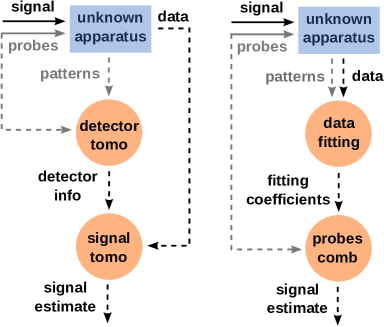
Figure 1: Information flow in standard tomography (left) and data-pattern tomography (right). Blue rectangles and orange circles represent the measurement and data processing steps. Solid and broken lines (in black for the signal and in grey for the probes) denote the propagation of physical systems and information, respectively.

In the standard approach, one uses the probes and patterns to characterize the unknown detector. Afterwards, the unknown state is estimated from data and the measurement matrix previously determined.

In the data-pattern tomography, the best fit of data with a linear combination of patterns is worked out and the same fit is used to combine the probes and form the signal estimate. In this way, the unknown state is expressed directly in terms of probes and their respective patterns, thus bypassing the (possibly costly) detector calibration. We note in passing that similar reasoning is at the heart of some neural networks for recognition systems [39].

We next examine both protocols from the viewpoint of lin estimation.

3.1 Standard tomography

In the first step, a set of $M$ known probes $\bi{r}_{\alpha}$ ($\alpha=1,\ldots,M$) is measured and their patterns $\bi{f}_{\alpha}$ collected. Arranging probes and patterns columnwise to form the matrices $R$ and $F$, of dimensions $m\times M$ and $n\times M$, respectively, we have to solve the problem

$$F=A\,R,$$ (3.1)

where the $m\times n$ matrix $A$ specifies the action of the detector. A lin estimation results in

$$A=FR^{+}.$$ (3.2)

The second step is to solve equation (2.2) for the signal $\mathbf{r}$. Substituting (3.2), we directly get the effective measurement matrix inverse for the standard tomography:

$$A_{s}=(FR^{+})^{+}\,.$$ (3.3)

Henceforth, we shall denote this approach by the subscript $s$.

3.2 Data-pattern tomography

With the same set of probes and patterns we now perform a data-pattern tomography. First, we do a linear fitting of the data with the patterns

$$\bi{f}=F\,\bi{x}\,,$$ (3.4)

where the fitting coefficients $\bi{x}$ are obtained with lin inversion; i.e.,

$$\bi{x}=F^{+}\,\bi{f}\,.$$ (3.5)

Because the linearity of the measurement, the same set of fitting coefficients can be used to expand the unknown state in known probes; i.e., $\bi{r}=R\,\bi{x}$. In this way, we train the protocol to recognize the probes and their linear combinations. Finally, using equation (3.5), we get that the effective measurement matrix inverse for the data-pattern LIN tomography reads

$$A_{p}=RF^{+}\,,$$ (3.6)

where the subscript $p$ designates this protocol.

4 Assessing the protocols

4.1 Reverse-order law

A simple glance at equations (3.3) and (3.6) immediately reveals that both protocols become equivalent provided that

$$(FR^{+})^{+}=RF^{+}\,.$$ (4.1)

This is obviously satisfied by proper matrix inverses, but not always by pseudoinverses. As sketched in the A, the identity (4.1) holds true if $F$ and $R$ have full column rank. This leads directly to our main result: lin standard tomography and lin data-pattern tomography are equivalent if all probes and all patterns are linearly independent.

The two protocols will differ if the number of probes and patterns is sufficiently large $M>\min\{m,n\}$. Particularly this covers the following important class of problems, namely

1. Informationally complete (IC) settings, where number of probe states $M$ is larger than the number of detected channels $m$, which equal (or larger) than the number of free parameters $n$ ($M>m\geq n$. As will be seen soon, when close to minimal tomography $m=n$, data pattern gives better results.

2. IC settings where the number of the output channels $m$ is larger (or equal) to number of probe states $M$, which in turn is larger than number of free parameters $m\geq M>n$. Here, the standard approach is more efficient.

3. Incomplete measurement, where number of free parameters $n$ exceeds the number of probe states $M$, which is larger than number of detected channels $n\geq M>m$. The equality (4.1) does not hold, but such measurements are not tomographically complete and will not be considered here.

4.2 Performances

Let us compare the performances of the two tomographic protocols for IC settings: $M,m\geq n$. There are two kinds of noise associated with both protocols: pattern noise and data noise. We assume that data noise dominates the reconstruction error. This assumption is justified by the very different roles played by the patterns and data in experimental tomography: patterns are collected for probe states. One would typically use simple states (i.e., easy to generate and calibrate) for probes. In general there is no restriction on how many copies of probe states can be used for probing the measurement setup. On the other hand, the unknown signal subject to reconstruction is typically a non-trivial/non-classical state and the number of available copies may be limited by the quantum information protocol used. Patterns can thus be expected to have better signal to noise ratio than signal data.

Denoting by $A_{\mathrm{true}}$ the true inversion matrix ($\bi{r}=A_{\mathrm{true}}\bi{p}$), and by $\Delta\bi{p}$ the data noise ($\bi{f}=\bi{p}+\Delta\bi{p}$), we can straightforwardly obtain the mean square error

$$e_{\alpha}^{2}=\overline{||A_{\alpha}\bi{f}-\bi{r}||^{2}}=\overline{||A_{\alpha}\bi{f}-A_{\mathrm{true}}\bi{p}||^{2}}\approx\overline{||A_{\alpha}\,\Delta\bi{p}||^{2}}=\frac{\epsilon^{2}\,||A_{\alpha}||^{2}}{m}\,.$$ (4.2)

Here, $\alpha\in\{s,p\}$, $||\bi{y}||^{2}=\Tr(\bi{y}^{\ast}\bi{y})$ is the Hilbert-Schmidt norm (the symbol $\ast$ denotes here the conjugate transpose), and the bar indicates averaging over all possible realizations of noise with a fixed strength $||\Delta\bi{p}||=\epsilon$. To get the last inequality, we note that for $||\Delta\bi{p}||=1$ the square norm $||A_{\alpha}\,\Delta\bi{p}||^{2}$ is constrained by the minimum and maximum eigenvalues of $A_{\alpha}^{\ast}A_{\alpha}$. Averaging over all $\Delta\bi{p}$ yields the aritmetic mean of eigenvalues, $\Tr(A_{\alpha}^{\ast}A_{\alpha})/m$. Incidentally, this can be considered as the first moment of a real numerical shadow [40] of the matrix product $A_{\alpha}^{\ast}A_{\alpha}$. For $\Delta\bi{p}$ of strength $\epsilon$, we obtain Eq. (4.2).

The discussion about the performance of both protocols thus boils down to a comparison of the norms of the corresponding inversion matrices, which decides the average performance of the protocol. Large norms indicate the tendency to amplify the noise present in the data and, therefore, such protocols should be avoided.

4.3 Limiting cases

We next examine two interesting limits that arise in practical experiments. We shall be making extensive use of a technical result [41] that provides a unique representation for the pseudoinverse of the product of any two matrices; viz,

$$(XY)^{+}=Y^{+}(h+g)X^{+}\,,$$ (4.3)

where $h=(X^{+}XYY^{+})^{+}$ is a (skew) projector and $g$ is a matrix with a number of special properties that the reader can check in the A, as well as other pertinent details.

4.3.1 $M>m=n$.

The measurement thus has the minimal number of outputs required for IC tomography, but the set of probes is (highly) redundant. Let us first assess the standard tomography. Now, equation (4.3) holds true with $g=0$; we have then

$$A_{s}=(FR^{+})^{+}=RhF^{+}\,,$$ (4.4)

with $h=(F^{+}FRR^{+})^{+}$. We use the singular value decomposition for $R$ as [42] as $R=U_{R}D_{R}V_{R}^{\ast}$ (with $D_{R}$ diagonal, $U_{R}^{\ast}U_{R}=\leavevmode\hbox{\small 1\normalsize\kern-3.30002pt1}$ and $V^{\ast}V=\leavevmode\hbox{\small 1\normalsize\kern-3.30002pt1}$), and analogously for $F$, and $h$. If we call $\mathcal{V}_{Rh}=V_{R}^{\ast}U_{h}$ and $\mathcal{V}_{hF}=V_{h}^{\ast}V_{F}$, we get

$$||A_{s}||=||S_{R}\mathcal{V}_{Rh}S_{h}\mathcal{V}_{hF}S_{F}^{+}||\,,$$ (4.5)

where we have introduced the square representations

$$S_{R}=\left(\begin{array}[]{cc}\!D_{R}&0\end{array}\right),\qquad S_{h}=\left(\begin{array}[]{cc}D_{h}&0\\ 0&0\end{array}\right)\,,\qquad S_{F}^{+}=\left(\begin{array}[]{c}D_{F}^{+}\\ 0\end{array}\right)\,,$$ (4.6)

all the $D$ blocks being $n\times n$ dimensional. The unitary matrices $\mathcal{V}_{Rh}$ and $\mathcal{V}_{hF}$ take the block diagonal form

$$\mathcal{V}_{Rh}=\left(\begin{array}[]{cc}U_{Rh}&0\\ 0&W_{Rh}\end{array}\right)\,,\qquad\mathcal{V}_{hF}=\left(\begin{array}[]{cc}U_{hF}&0\\ 0&W_{hF}\end{array}\right),$$ (4.7)

with $U_{Rh},U_{hF}$ and $W_{Rh},W_{hF}$ being $n\times n$ and $(M-n)\times(M-n)$ dimensional, respectively. Consequently,

$$||A_{s}||=||D_{R}U_{Rh}D_{h}U_{hF}D_{F}||\,,$$ (4.8)

and $||U_{Rh}D_{h}U_{hF}||=||D_{h}||\geq\sqrt{n}$.

Repeating the calculation for the pattern tomography, we obtain

$$||A_{p}||=||D_{R}U_{11}D_{F}||\,,$$ (4.9)

where $U_{11}$ is the corresponding matrix element of $V_{R}^{\ast}V_{F}$, and satisfies $|U_{11}|\leq\sqrt{n}$.

Of course, the fact that the matrix sandwiched between $D_{R}$ and $D_{F}$ in (4.8) has a greater norm than that in (4.9) does not imply $||A_{s}||\geq||A_{p}||$. However, with increasing $M$, and hence decreasing $|U_{11}|$ relative to $||D_{h}||$, this is likely to happens and is confirmed in our numerical simulations. Loosely speaking, the block diagonal form of $\mathcal{V}_{Rh}$ and $\mathcal{V}_{hF}$ prevents the scattering of the nonzero singular values of $S_{F}^{+}$ into the nullspace of $S_{R}$, which tends to increase the norm of the standard inversion matrix, and, consequently $e_{s}\geq e_{p}$.

We thus conclude that for minimal measurements and highly redundant set of probes, we expect the lin data-pattern tomography to outperform the lin standard tomography and the difference grows with the number of probes $M$.

4.3.2 $m\geq M>n$.

Now, the measurement is not minimal and the number of probes does not exceed the number of measurement outputs. The matrix of patterns $F$ has full column rank, the corresponding projector $F^{+}F$ is a unity matrix and, in consequence, $h=(R^{+}R)^{+}=R^{+}R$:

$$A_{s}=R(R^{+}R+g)F^{+}\,.$$ (4.10)

By the properties of $g$, and more concretely (1.4), we have

$$||A_{s}||=||R(R^{+}R+g)F^{+}||\leq||RF^{+}||=||A_{p}||$$ (4.11)

and $e_{s}\leq e_{p}$. Hence, for highly complex measurements, we expect the standard detector tomography to be more efficient than the data-pattern approach.

To sump up, choosing a fixed $m\geq n$ and increasing the number of probes from $M=n$, the data pattern tomography, initially the worse technique, becomes superior for large probe numbers $M\gg n$.

5 Examples

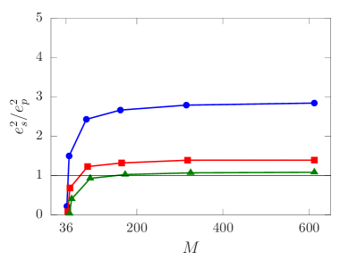
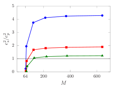
Figure 2: Performance ratios in dimension $d=6$ ($n=35$, left) and $d=8$ ($n=63$, right). Random square-root measurements with $m=n+3$ (blue circles), $m=n+5$ (red squares), and $m=n+9$ (green triangles) outputs are simulated.

To confirm our conclusions we have performed simulations of quantum state tomography with random square-root measurements

$$\Pi_{j}=G^{-1/2}|\phi_{j}\rangle\langle\phi_{j}|G^{-1/2}\,,\qquad G=\sum_{j}|\phi_{j}\rangle\langle\phi_{j}|\,,$$ (5.1)

where $|\phi_{j}\rangle$ are randomly generated Haar-distributed pure states (aka random states) and $j=1,\ldots,m$. This scheme has been proposed as a pretty good’ measurement for distinguishing quantum states [43] and is known to be optimal [44].

For each measurement we generate a set of $M$ random probes and the corresponding patterns. The simulated data is obtained for a set of 10000 random true states and the mean square errors are computed from the estimates. Finally, to quantify the performance, we average $e_{s}^{2}$ and $e_{p}^{2}$ over several hundred random square-root measurements. The system dimension $d$ is fixed to be 6 or 8 (which means $n=d^{2}-1$ is 35 and 63, respectively) and the noise was simulated by adding Gaussian noise to the theoretically calculated detection probabilities. The noise-to-signal ratio was set $0.03$ and $0.06$ for the patterns and data, respectively.

The first set of simulations in figure 2 shows the dependence of the performance ratio $e_{s}^{2}/e_{p}^{2}$ on the number of probes for three different measurement outputs $m$. In a remarkable agreement with the theory, the data-pattern approach performs poorly when $m=M$, but considerably improves when the number of probes increases; and this is more pronounced for higher dimensions.

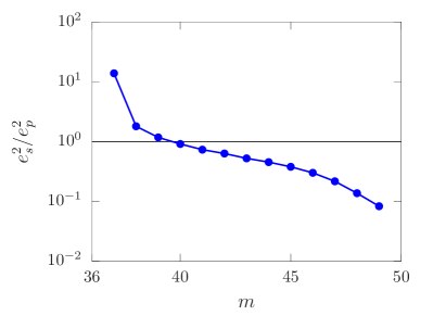
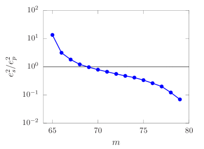
Figure 3: Performance ratios for random square-root measurements in dimension $d=6$ with $M=50$ probes (left), and dimenson $d=8$ and $M=80$ probes (right).

In figure 3, we plot the same ratio $e_{s}^{2}/e_{p}^{2}$, but now keeping $M$ fixed and varying $m$. The data-pattern approach is better for minimal and nearly minimal schemes $m\approx n$, whereas the standard tomography is recommended for highly complex measurements $m\gg n$.

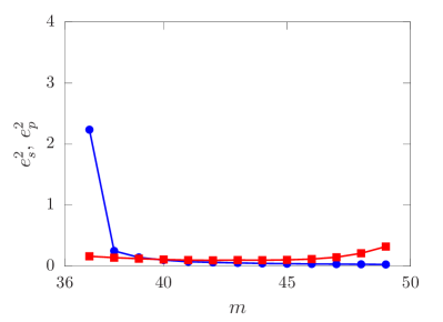
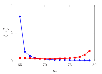
Figure 4: Mean square errors for random square-root measurements with the standard (blue circles) and data pattern (red squares) protocols in dimension $d=6$ ($n=35$ and $M=50$, left), and $d=8$ ($n=63$ and $M=80$, right).

Figure 4 shows the mean square errors for the two protocols. With a fixed number of probes, the reconstruction error of the standard scheme decreases with increasing $m$: more measurement outputs make the overall reconstruction error smaller. For the data-pattern approach, this tendency is much the opposite.

We also simulated realistic homodyne detection. For this end, we have used coherent states as probes, as they are easy to generate. In our simulations we use of $M=100$ randomly generated coherent states with amplitudes $|\alpha|<0.8$. The states are calibrated and their amplitudes are known to the experimenter. The true unknown state to be reconstructed is chosen to be the following coherent superposition (in the Fock basis )

$$|\Psi_{\mathrm{true}}\rangle=\sqrt{0.1}\,|0\rangle+\sqrt{0.2}\,|1\rangle+\sqrt{0.3}\,|2\rangle\,.$$ (5.2)

We set the quantum efficiency of the homodyne detection to $80\%$ and generate $m$ random quadrature measurements of the signal and probe states. The data-pattern tomography and standard tomography are used to reconstruct the unknown signal in the subspace spanned by the Fock states $|0\rangle,|1\rangle,\ldots,|5\rangle$, so that $n=35$.

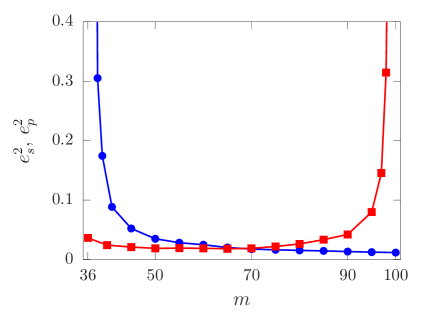
Figure 5: Mean square errors of standard (blue circles) and data-pattern (red squares) protocols in the Fock subspace of dimension six ($n=35$). State averaged errors are shown for a randomly generated inefficient homodyne measurement with $\eta=0.8$, and $M=100$.

As one can observe in figure 5, the mean square errors display two prominent resonant-like peaks at $m=n$ and $m=M$, where one protocol clearly outperforms the other. This can be illustrated further with the Wigner representations of the measured signal obtained in those two extreme regimes, shown in figure 6. For example, for the minimal IC setting $m=n$, the repeated data-pattern reconstructions are all very good, while the standard tomography delivers results ranging from reasonably good to very bad.

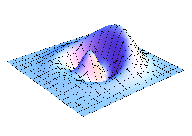
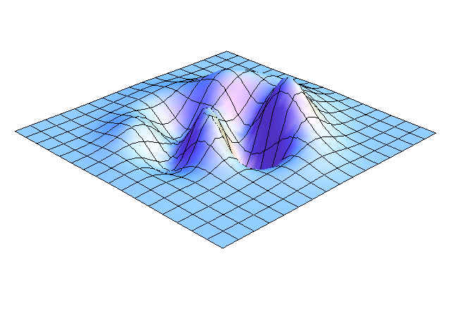
Figure 6: Typical reconstructions by data-pattern tomography with $m=n=35$ (left) and $m=M=100$ (right). In the minimal IC setting the reconstruction is very good (in fact, almost identical to the Wigner function for the true state, with strong negativity witnessing the nonclassical character), while it is very bad in the other opposite limit. The reverse behavior, with almost the same figures interchanged, is observed for the standard approach, although the figures are not reproduced here for simplicity.

6 Conclusions

In summary, we have found substantial differences in the performance of the two protocols traditionally used for estimating the state of a physical system from unknown measurements. This is important from a practical point of view, as obtaining good results strongly depends on choosing the correct estimation strategy. In particular, the data-pattern approach yields better results for minimal measurement settings, whereas the standard approach is better suited to handle complex overcomplete measurements. These differences can be ascribed to different order in which the information available is processed to get the final signal estimate. Since we deal with matrices, the order of utilizing information about probes and patterns does matter.

Although our theory and simulations have been worked out solely for the simple linear estimator, we expect to see similar effects should a more sophisticated nonlinear inference, such as the maximum-likelihood estimation, be adopted. This is the subject of further investigations.

Appendix A The Moore-Penrose pseudoinverse

In these appendix we give a brief account of the Moore-Penrose pseudoinverse. The interested reader can find more details in the comprehensive references [45] and [46].

For any $m\times n$ matrix $X$, its pseudoinverse $X^{+}$ must satisfy all the following conditions [47]

1. $XX^{+}X=X$

2. $X^{+}XX^{+}=X^{+}$

3. ($XX^{+})^{\ast}=XX^{+}$

4. ($X^{+}X)^{\ast}=X^{+}X$

Here $\ast$ denotes the conjugate transpose. This provides a quick checkable criterion; that is, given a matrix $G$ that purports to be the pseudoinverse of $X$, one need simply verify the four conditions C1–C4 above. This verification is often relatively straightforward. We stress that the pseudoinverse always exists and is unique.

Alternatively, $X^{+}$ can be defined as the limit

$$X^{+}=\lim_{\delta\rightarrow 0}(X^{\ast}X+\delta\leavevmode\hbox{\small 1\normalsize\kern-3.30002pt1})^{-1}X^{\ast}=\lim_{\delta\rightarrow 0}X^{\ast}(XX^{\ast}+\delta\leavevmode\hbox{\small 1\normalsize\kern-3.30002pt1})^{-1}\,.$$ (1.1)

We next quote a few useful properties:

1. $X^{+}=(X^{\ast}X)^{+}X^{\ast}=X^{\ast}(XX^{\ast})^{+}$

2. $(X^{\ast})^{+}=(X^{+})^{\ast}$

3. $(X^{+})^{+}=X$

4. $(X^{\ast}X)^{+}=X^{+}(X^{\ast})^{+},\quad(XX^{\ast})^{+}=(X^{\ast})^{+}X^{+}$

5. $\mathcal{R}(X^{+})=\mathcal{R}(X^{+}X)=\mathcal{R}(X^{t}),\quad\mathcal{N}(X^{+})=\mathcal{N}(XX^{+})=\mathcal{N}(X^{t})$

where $\mathcal{R}$ denotes the range and $\mathcal{N}$ the null subspace of the corresponding matrix, and the superscript $t$ stands for the transpose.

If $X$ is $m\times n$ and $Y$ is $n\times p$ and either: $X$ has orthonormal columns, or $Y$ has orthonormal rows, or $X$ has full column rank and $Y$ has full row rank, or $Y=X^{\ast}$, then

$$(XY)^{+}=Y^{+}X^{+}\,.$$ (1.2)

In the general case, however, the analytical structure of the Moore-Penrose pseudoinverse of the product of any two matrices is more complex. It has been fully specified by Galperin and Waksman [41], and the following theorem has been extensively used in our paper:

Theorem 1

Let $X$ and $Y$ be two arbitrary matrices, and $h=(X^{+}XYY^{+})^{+}$. Then there exists a unique matrix $g$ such that

$$(XY)^{+}=Y^{+}(h+g)X^{+}\quad\&\quad YY^{+}gX^{+}X=g\,.$$ (1.3)

It holds that $g\perp h$ and of all $z$ satisfying $YY^{-}zX^{+}X=z$ and $XzY=0$, $g$ makes $||Y^{+}(h+z)X^{+}||$ minimum. In particular, this means that

$$||Y^{+}(h+g)X^{+}||\leq||Y^{+}hX^{+}||\,.$$ (1.4)

The projector $h$ has many interesting properties. It holds true that

$$\begin{array}[]{l}\mathcal{R}(h)=\mathcal{R}(Y)\cap[\mathcal{R}(X^{\ast})+\mathcal{N}(Y^{\ast})]\,,\\ \mathcal{N}(h)=\mathcal{R}(X^{\ast})\cap\mathcal{N}(Y^{\ast})+\mathcal{N}(X)\,.\end{array}$$ (1.5)

These properties have played a crucial role in our estimates in section 4.3.

References

- [1] Groetsch C W 1993 Inverse Problems in the Mathematical Sciences (Wiesbaden: Springer Vieweg)
- [2] Tarantola A 2005 Inverse Problem Theory and Methods for Model Parameter Estimation (Philadelphia: SIAM)
- [3] Aster R, Borchers B and Thurber C 2013 Parameter Estimation and Inverse Problems 2nd ed (Boston: Academic)
- [4] Luis A and Sánchez-Soto L L 1999 Phys. Rev. Lett. 83 3573–3576
- [5] Fiurášek J 2001 Phys. Rev. A 64 024102
- [6] D’Ariano G M, Maccone L and Lo Presti P 2004 Phys. Rev. Lett. 93 250407
- [7] Lundeen J S, Feito A, Coldenstrodt-Ronge H, Pregnell K L, Silberhorn C, Ralph T C, Eisert J, Plenio M B and Walmsley I A 2009 Nat. Phys. 5 27–30
- [8] Zhang L, Datta A, Coldenstrodt-Ronge H B, Jin X M, Eisert J, Plenio M B and Walmsley I A 2012 New J. Phys. 14 115005
- [9] D’Auria V, Lee N, Amri T, Fabre C and Laurat J 2011 Phys. Rev. Lett 107 050504
- [10] Zhang L, Coldenstrodt-Ronge H B, Datta A, Puentes G, Lundeen J S, Jin X M, Smith B J, Plenio M B and Walmsley I A 2012 Nat Photon 6 364–368
- [11] Feito A, Lundeen J S, Coldenstrodt-Ronge H, Eisert J, Plenio M B and Walmsley I A 2009 New J. Phys. 11 093038
- [12] Coldenstrodt-Ronge H B, Lundeen J S, Pregnell K L, Feito A, Smith B J, Mauerer W, Silberhorn C, Eisert J, Plenio M B and Walmsley I A 2009 J. Mod. Opt. 56 432–441
- [13] Brida G, Ciavarella L, Degiovanni I P, Genovese M, Lolli L, Mingolla M G, Piacentini F, Rajteri M, Taralli E and Paris M G A 2012 New J. Phys. 14 085001
- [14] Akhlaghi M K, Majedi A H and Lundeen J S 2011 Opt. Express 19 21305–21312
- [15] Renema J J, Frucci G, Zhou Z, Mattioli F, Gaggero A, Leoni R, de Dood M J A, Fiore A and van Exter M P 2012 Opt. Express 20 2806–2813
- [16] Renema J J, Gaudio R, Wang Q, Zhou Z, Gaggero A, Mattioli F, Leoni R, Sahin D, de Dood M J A, Fiore A and van Exter M P 2014 Phys. Rev. Lett. 112 117604
- [17] Klyshko D N 1980 Sov. J. Quantum Electron. 10 1112–1117
- [18] Worsley A P, Coldenstrodt-Ronge H B, Lundeen J S, Mosley P J, Smith B J, Puentes G, Thomas-Peter N and Walmsley I A 2009 Opt. Express 17 4397–4412
- [19] Avella A, Brida G, Degiovanni I P, Genovese M, Gramegna M, Lolli L, Monticone E, Portesi C, Rajteri M, Rastello M L, Taralli E, Traina P and White M 2011 Opt. Express 19 23249–23257
- [20] Yang T H, Vértesi T, Bancal J D, Scarani V and Navascués M 2014 Phys. Rev. Lett. 113 040401
- [21] Wu X, Bancal J D, McKague M and Scarani V 2016 Phys. Rev. A 93 062121
- [22] Chen S L, Budroni C, Liang Y C and Chen Y N 2016 Phys. Rev. Lett. 116 240401–
- [23] Mogilevtsev D, Řeháček J and Hradil Z 2009 Phys. Rev. A 79 020101
- [24] Mogilevtsev D 2010 Phys. Rev. A 82 021807
- [25] Brańczyk A M, Mahler D H, Rozema L A, Darabi A, Steinberg A M and James D F V 2012 New J. Phys. 14 085003
- [26] Mogilevtsev D, Řeháček J and Hradil Z 2012 New J. Phys. 14 095001
- [27] Stark C J 2016 Commun. Math. Phys. 348 1–25
- [28] Řeháček J, Mogilevtsev D and Hradil Z 2010 Phys. Rev. Lett. 105 01040
- [29] Mogilevtsev D, Ignatenko A, Maloshtan A, Stoklasa B, Rehacek J and Hradil Z 2013 New J. Phys. 15 025038
- [30] Cooper M, Karpinski M and Smith B J 2013 arxiv:1306.6431
- [31] Harder G, Silberhorn C, Rehacek J, Hradil Z, Motka L, Stoklasa B and Sánchez-Soto L L 2014 Physical Review A 90 042105
- [32] Altorio M, Genoni M G, Somma F and Barbieri M 2016 Phys. Rev. Lett. 116 100802
- [33] Lawson C and Hanson R 1974 Solving Least Squares Problems (Englewood Cliffs: Prentice-Hall)
- [34] Hallin M 2006 Gauss–Markov Theorem in Statistics (John Wiley & Sons) ISBN 9781118445112
- [35] Kay S M 1993 Fundamentals of Statistical Processing: Estimation Theory (New Jersey: Prentice Hall)
- [36] Millar R B 2011 Maximum Likelihood Estimation and Inference (Chichester: Wiley)
- [37] Gelman A, Carlin J B, Stern H S and Dunson D B 2013 Bayesian Data Analysis 3rd ed (Boca Raton: CRC Press)
- [38] Kimura G 2003 Phys. Lett. A 314 339–349
- [39] Bishop C M 1995 Neural Networks for Pattern Recognition (Oxford: Oxford University Press)
- [40] Puchała Z, Miszczak J A, Gawron P, Dunkl C F, Holbrook J A and Życzkowski K 2012 J. Phys. A: Math. Theor. 45 415309
- [41] Galperin A M and Waksman Z 1980 Linear Algebra Appl. 33 123–131
- [42] Golub G and Kahan W 1965 SIAM J. Numer. Anal. 2 205–224
- [43] Hausladen P and Wootters W K 1994 J. Mod. Opt. 41 2385–2390
- [44] Dalla Pozza N and Pierobon G 2015 Physical Review A 91 042334–
- [45] Ben-Israel A and Greville T N E 1977 Generalized Inverses: Theory and Applications (New York: Wiley)
- [46] Campbell S L and Meyer C D J 1991 Generalized Inverses of Linear Transformations (New York: Dover)
- [47] Penrose R 1955 Proc. Cambridge Phil. Soc. 51 406–413