LAGRANGIAN DESCRIPTORS FOR STOCHASTIC DIFFERENTIAL EQUATIONS: A TOOL FOR REVEALING THE PHASE PORTRAIT OF STOCHASTIC DYNAMICAL SYSTEMS

Abstract

In this paper we introduce a new technique for depicting the phase portrait of stochastic differential equations. Following previous work for deterministic systems, we represent the phase space by means of a generalization of the method of Lagrangian descriptors to stochastic differential equations. Analogously to the deterministic differential equations setting, the Lagrangian descriptors graphically provide the distinguished trajectories and hyperbolic structures arising within the stochastic dynamics, such as random fixed points and their stable and unstable manifolds. We analyze the sense in which structures form barriers to transport in stochastic systems. We apply the method to several benchmark examples where the deterministic phase space structures are well-understood. In particular, we apply our method to the noisy saddle, the stochastically forced Duffing equation, and the stochastic double gyre model that is a benchmark for analyzing fluid transport.

Keywords: Stochastic differential equation, Lagrangian descriptor, distinguished trajectories, hyperbolicity, random fixed point, stable and unstable manifolds.

1 Introduction

In recent years Lagrangian descriptors (LD) have been shown to be a useful technique for discovering phase space structure in both autonomous and nonautonomous dynamical systems. In chaos Lagrangian descriptors (also referred to in the literature as the “M function”) were used to discover hyperbolic trajectories and their stable and unstable manifolds in aperiodically time dependent vector fields. In particular, this paper considers “important hyperbolic trajectories”, referred to as distinguished trajectories, which build on the well-known idea of distinguished hyperbolic trajectory, discussed earlier in kayo .

Lagrangian descriptors can easily be applied to the analysis of velocity fields defined as data sets. Early work demonstrating this was concerned with transport associated with the Kuroshio current, described in prl ; jfm . This work set the stage for further geophysical transport studies described in, for example, amism11 ; alvaro2 . An application concerned with determining the connection between coherent structures and the saturation of a nonlinear dynamo is described in rempel . More recently, Lagrangian descriptors have been used to analyze issue related to the search strategy for the Malaysian airliner MH370 GMWM15 as well as to an understanding of events surrounding the Deepwater Horizon oil spill (mmw14 ) and, more recently, to an analysis of the real time development of an oil spill in the Canary Islands GRMCW15 .

In cnsns a general assessment of Lagrangian descriptors was carried out. Different Lagrangian descriptors were considered and applied to a variety of benchmark examples containing known phase space structures. While most of the previous applications of Lagrangian descriptors had been to two dimensional, time dependent flows, it was also shown that dimensionality is not a restriction to the application of the method. In particular, transport associated with the three dimensional time dependent Hill’s spherical vortex was considered. The computational requirements of Lagrangian descriptors were also considered and compared with those of finite time Lyapunov exponents (FTLEs).

The applications of Lagrangian descriptors mentioned above are in areas of fluid mechanics. However, the method of Lagrangian descriptors applies to general vector fields in $n$ dimensions, and there is no obstacle to using Lagrangian descriptors for applications in a higher dimensional setting. Recently, this has been illustrated by a series of applications of Lagrangian descriptors to problems in chemistry by Hernandez and co-workers. In particular, they have applied Lagrangian descriptors to a study of chemical reactions under external time-dependent driving in CH15 , barrierless reactions in JH16 ; JH2016 , and ketene isomerization in CH16 . Finally, we remark that the use of Lagrangian descriptors for visualizing phase space structures in complex dynamical systems is described in MCWGM15 .

In this paper we continue the development of the method of Lagrangian descriptors by carrying it out in the setting of stochastic differential equations. This provides us with a computational tool for revealing the phase space structure of stochastic dynamical systems. We will discuss in detail what this means by considering explicit examples and comparing them with their deterministic counterparts.

This paper is organized as follows: in Section 2 we give a brief summary of preliminary concepts as well as set the general framework of stochastic differential equations. In Section 3 we define Stochastic Lagrangian descriptor (SLD) as a method to reveal the phase space of a stochastic system and in Section 4 we describe the numerical method used to implement SLD. Finally in Section 6, we compute the SLD by using some benchmark examples: the noisy saddle system, the stochastic versions of the Duffing equation, and the stochastic Double Gyre.

2 Preliminary concepts

The general framework in which Lagrangian descriptors (in their stochastic version) are defined, requires us to carefully describe the nature of solutions of a stochastic differential equation (SDE). Therefore, to begin we consider a general system of SDEs expressed in differential form as follows:

$$dX_{t}=b(X_{t},t)dt+\sigma(X_{t},t)dW_{t},\quad t\in\mathbb{R},$$ (1)

where $b(\cdot)\in C^{1}(\mathbb{R}^{n}\times\mathbb{R})$ is the deterministic part, $\sigma(\cdot)\in C^{1}(\mathbb{R}^{n}\times\mathbb{R})$ is the random forcing, $W_{t}$ is a Wiener process (also called Brownian motion) whose definition is given later, and $X_{t}$ is the solution of the equation. All these functions take values in $\mathbb{R}^{n}$.

As the notion of solution of a SDE is closely related with the Wiener process, we state what is meant by $W(\cdot)$. This definition is given in duan15 , and this reference serves to provide the background for all of the notions in this section. Also, throughout this article we will use $\Omega$ to denote the probability space where the Wiener process is defined.

Definition 2.1.

A real valued stochastic Wiener or Brownian process $W(\cdot)$ is a stochastic process defined in a probability space $(\Omega,{\cal F},{\cal P})$ which satisfies

1. $W_{0}=0$ (standard Brownian motion),

2. $W_{t}-W_{s}$ follows a Normal distribution $N(0,t-s)$ for all $t\geq s\geq 0$,

3. for all time $0<t_{1}<t_{2}<...<t_{n}$, the random variables $W_{t_{1}},W_{t_{2}}-W_{t_{1}},...,W_{t_{n}}-W_{t_{n-1}}$ are independent (independent increments).

Moreover, $W(\cdot)$ is a real valued two-sided Wiener process if conditions (ii) and (iii) change into

1. $W_{t}-W_{s}$ follows a Normal distribution $N(0,|t-s|)$ for all $t,s\in\mathbb{R}$,

2. for all time $t_{1},t_{2},...,t_{2n}\in\mathbb{R}$ such that the intervals $\{(t_{2i-1},t_{2i})\}_{i=1}^{n}$ are non-intersecting between them, the random variables $W_{t_{1}}-W_{t_{2}},W_{t_{3}}-W_{t_{4}},...,W_{t_{2n-1}}-W_{t_{2n}}$ are independent.

As it is mentioned in the introduction, the purpose of this article is to develop the method of Lagrangian descriptors for SDEs. This method of Lagrangian descriptors has been developed for deterministic differential equations whose temporal domain is $\mathbb{R}$. In this sense it is natural to work with two-sided solutions as well as two-sided Wiener processes. Henceforth, every Wiener process $W(\cdot)$ considered in the this article will be of this form.

Given that any Wiener process $W(\cdot)$ is a stochastic process, by definition this is a family of random real variables $\{W_{t},t\in\mathbb{R}\}$ in such a way that for each $\omega\in\Omega$ there exists a mapping

$$t\longmapsto W_{t}(\omega)$$

known as the trajectory of a Wiener process.

Analogously to the Wiener process, the solution $X_{t}$ of the SDE (1) is also a stochastic process. In particular, it is a family of random variables $\{X_{t},t\in\mathbb{R}\}$ such that for each $\omega\in\Omega$, the trajectory of $X_{t}$ satisfies

$$t\longmapsto X_{t}(\omega)=X_{0}(\omega)+\int_{0}^{t}b(X_{s}(\omega),s)ds+\int_{0}^{t}\sigma(X_{s}(\omega),s)dW_{s}(\omega),$$ (2)

where $X_{0}\mathrel{\mathop{\mathchar 58\relax}}\Omega\rightarrow\mathbb{R}^{n}$ is the initial condition. In addition, as $b(\cdot)$ and $\sigma(\cdot)$ are smooth functions, they are locally Lipschitz and this leads to existence and pathway uniqueness of a local, continuous solution (see duan15 ). That is if any two stochastic processes $X^{1}$ and $X^{2}$ are local solutions in time of SDE (1), then $X^{1}_{t}(\omega)=X^{2}_{t}(\omega)$ over a time interval $t\in(t_{i},t_{f})$ and for almost every $\omega\in\Omega$.

At each instant of time $t$, the deterministic integral $\int_{0}^{t}b(X_{s}(\omega))ds$ is defined by the usual Riemann integration scheme since $b$ is assumed to be a differentiable function. However, the stochastic integral term is chosen to be defined by the Itô integral scheme:

$$\int_{0}^{t}\sigma(X_{s}(\omega),s)dW_{s}(\omega)=\lim_{N\rightarrow\infty}\sum_{i=0}^{N-1}\sigma(X_{i\frac{t}{N}}(\omega),it/N)\cdot\left[W_{(i+1)\frac{t}{N}}(\omega)-W_{i\frac{t}{N}}(\omega)\right].$$ (3)

This scheme will also facilitate the implementation of a numerical method for computing approximations for the solution $X_{t}$ in the next section.

Once the notion of solution, $X_{t}$, of a SDE (1) is established, it is natural to ask if the same notions and ideas familar from the study of deterministic differential equations from the dynamical systems point of view are still valid for SDEs. In particular, we want to consider the notion of hyperbolic trajectory and its stable and unstable manifolds in the context of SDEs. We also want to consider how such notions would manifest themselves in the context of phase space transport for SDEs, and the stochastic Lagrangian descriptor will play a key role in considering these questions from a practical point of view.

We first discuss the notion of an invariant set for a SDE. In the deterministic case the simplest possible invariant set is a single trajectory of the differential equation. More precisely, it is the set of points through which a solution passes. Building on this construction, an invariant set is a collection of trajectories of different solutions. This is the most basic way to characterize the invariant sets with respect to a determinsitic differential equation of the form

$$\dot{x}=f(x,t),\quad x\in\mathbb{R}^{n},\quad t\in\mathbb{R}.$$ (4)

For verifying the invariance of such sets the solution mapping generated by the vector field is used. For deterministic autonomous systems these are referred to as flows (or ‘’dynamical systems”) and for deterministic nonautonomous systems they are referred to as processes. The formal definitions are in Appendix 1 and can also be found in kloe11 .

A similar notion of solution mapping for SDEs is introduced using the notion of a random dynamical system $\varphi$ (henceforth referred to as RDS) in the context of SDEs. This function $\varphi$ is also a solution mapping of a SDE that satisfies several conditions, but compared with the solution mappings in the deterministic case, this RDS depends on an extra argument which is the random variable $\omega\in\Omega$. Furthermore the random variable $\omega$ evolves with respect to $t$ by means of a dynamical system $\{\theta_{t}\}_{t\in\mathbb{R}}$ defined over the probability space $\Omega$.

Definition 2.2.

Let $\{\theta_{t}\}_{t\in\mathbb{R}}$ be a measure-preserving dynamical system defined over $\Omega$, and let $\varphi\mathrel{\mathop{\mathchar 58\relax}}\mathbb{R}\times\Omega\times\mathbb{R}^{n}\rightarrow\mathbb{R}^{n}$ be a measurable mapping such that $(t,\cdot,x)\mapsto\varphi(t,\omega,x)$ is continuous for all $\omega\in\Omega$, and the family of functions $\{\varphi(t,\omega,\cdot)\mathrel{\mathop{\mathchar 58\relax}}\mathbb{R}^{n}\rightarrow\mathbb{R}^{n}\}$ has the cocycle property:

$$\varphi(0,\omega,x)=x\quad\text{and}\quad\varphi(t+s,\omega,x)=\varphi(t,\theta_{s}\omega,\varphi(s,\omega,x))\quad\text{for all }t,s\in\mathbb{R},\text{ }x\in\mathbb{R}^{n}\text{ and }\omega\in\Omega.$$

Then the mapping $\varphi$ is a random dynamical system with respect to the stochastic differential equation

$$dX_{t}=b(X_{t})dt+\sigma(X_{t})dW_{t}$$

if $\varphi(t,\omega,x)$ is a solution of the equation.

Analogous to the deterministic case, the definition of invariance with respect to a SDE can be characterized in terms of a RDS. This is an important topic in our consideration of stochastic Lagrangian descriptors. Now we introduce an example of a SDE for which the analytical expression of the RDS is obtained. This will be a benchmark example in our development of stochastic Lagrangian descriptors their relation to stochastic invariant manifolds.

Example 2.3.

(Noisy saddle point)

For the stochastic differential equation

$$\begin{cases}dX_{t}=X_{t}dt+dW_{t}^{1}\\ dY_{t}=-Y_{t}dt+dW_{t}^{2}\end{cases}$$ (5)

where $W_{t}^{1}$ and $W_{t}^{2}$ are two different Wiener processes, the solutions take the expressions

$$X_{t}=e^{t}\left(X_{0}(\omega)+\int_{0}^{t}e^{-s}dW_{s}^{1}(\omega)\right)\quad,\quad Y_{t}=e^{-t}\left(Y_{0}(\omega)+\int_{0}^{t}e^{s}dW_{s}^{2}(\omega)\right)$$ (6)

and therefore the random dynamical system $\varphi$ takes the form

$$\begin{array}[]{ccccccccc}\varphi\mathrel{\mathop{\mathchar 58\relax}}&&\mathbb{R}\times\Omega\times\mathbb{R}^{2}&&\longrightarrow&&\mathbb{R}^{2}&&\\ &&(t,\omega,(x,y))&&\longmapsto&&\left(\varphi_{1}(t,\omega,x),\varphi_{2}(t,\omega,y)\right)&=&\left(e^{t}\left(x+\int_{0}^{t}e^{-s}dW_{s}^{1}(\omega)\right),e^{-t}\left(y+\int_{0}^{t}e^{s}dW_{s}^{2}(\omega)\right)\right).\end{array}$$ (7)

Notice that this last definition (2.2) is expressed in terms of SDEs with time-independent coefficients $b,\sigma$. For more general SDEs we introduce a definition of nonautonomous RDS in Appendix 2, inspired in Definition 7.2 of processes for deterministic nonautonomous differential equations in Appendix 1. However, for the remaining examples considered in this article we make use of the already given definition of RDS.

Once we have the notion of RDS, it can be used to describe and detect geometrical structures and determine their influence on the dynamics of trajectories. Specifically, in clear analogy with the deterministic case, we focus on those trajectories whose expressions do not depend explicitly on time $t$, which are referred as random fixed points. Moreover, their stable and unstable manifolds, which may also depend on the random variable $\omega$, are also objects of interest due to their influence on the dynamical behavior of nearby trajectories. Both types of objects are invariant. Therefore we describe a characterization of invariant sets with respect to a SDE by means of an associated RDS.

Definition 2.4.

A non empty collection $M\mathrel{\mathop{\mathchar 58\relax}}\Omega\rightarrow\mathcal{P}(\mathbb{R}^{n})$, where $M(\omega)\subseteq\mathbb{R}^{n}$ is a closed subset for every $\omega\in\Omega$, is called an invariant set for a random dynamical system $\varphi$ if

$$\varphi(t,\omega,M(\omega))=M(\theta_{t}\omega)\quad\text{for every }t\in\mathbb{R}\text{ and every }\omega\in\Omega.$$ (8)

Again, we return to the noisy saddle (5), which is an example of a SDE for which several invariant sets can be easily characterized by means of its corresponding RDS.

Example 2.5.

(Noisy saddle point) For the stochastic differential equations

$$\begin{cases}dX_{t}=X_{t}dt+dW_{t}^{1}\\ dY_{t}=-Y_{t}dt+dW_{t}^{2}\end{cases}$$ (9)

where $W_{t}^{1}$ and $W_{t}^{2}$ are two different Wiener processes, the solution mapping $\varphi$ is given by the following expression

$$\begin{array}[]{ccccccccc}\varphi\mathrel{\mathop{\mathchar 58\relax}}&&\mathbb{R}\times\Omega\times\mathbb{R}^{2}&&\longrightarrow&&\mathbb{R}^{2}&&\\ &&(t,\omega,(x,y))&&\longmapsto&&(\varphi_{1}(t,\omega,x),\varphi_{2}(t,\omega,y))&=&\left(e^{t}\left(x+\int_{0}^{t}e^{-s}dW_{s}^{1}(\omega)\right),e^{-t}\left(y+\int_{0}^{t}e^{s}dW_{s}^{2}(\omega)\right)\right).\end{array}$$

Notice that this is a decoupled random dynamical system. There exists a solution whose components do not depend on variable $t$ and are convergent for almost every $\omega\in\Omega$ as a consequence of the properties of Wiener processes (see duan15 ). This solution has the form:

$$\tilde{X}(\omega)=(\tilde{x}(\omega),\tilde{y}(\omega))=\left(-\int_{0}^{\infty}e^{-s}dW_{s}^{1}(\omega),\int_{-\infty}^{0}e^{s}dW_{s}^{2}(\omega)\right).$$

Actually, $\tilde{X}(\omega)$ is a solution because it satisfies the invariance property that we now verify:

$$\begin{array}[]{ccl}\varphi_{1}(t,\omega,\tilde{x}(\omega))&=&\displaystyle{e^{t}\left(-\int_{0}^{+\infty}e^{-s}dW^{1}_{s}(\omega)+\int_{0}^{t}e^{-s}dW^{1}_{s}(\omega)\right)}=\displaystyle{-\int_{t}^{+\infty}e^{-(s-t)}dW^{1}_{s}(\omega)}\\ &=&\displaystyle{-\int_{0}^{+\infty}e^{-t^{\prime}}dW^{1}_{t^{\prime}+t}(\omega)=-\int_{0}^{+\infty}e^{-t^{\prime}}dW^{1}_{t^{\prime}}(\theta_{t}\omega)=\tilde{x}(\theta_{t}\omega)}\quad\text{by means of }t^{\prime}=s-t,\end{array}$$ (10)

$$\begin{array}[]{lll}\varphi_{2}(t,\omega,\tilde{y}(\omega))&=&\displaystyle{e^{-t}\left(\int_{-\infty}^{0}e^{s}dW^{2}_{s}(\omega)+\int_{0}^{t}e^{s}dW^{2}_{s}(\omega)\right)=\int_{-\infty}^{t}e^{s-t}dW^{2}_{s}(\omega)=\int_{-\infty}^{0}e^{t^{\prime}}dW^{2}_{t^{\prime}+t}(\omega)}\\ &=&\displaystyle{\int_{-\infty}^{0}e^{t^{\prime}}dW^{2}_{t^{\prime}}(\theta_{t}\omega)=\tilde{y}(\theta_{t}\omega)}\quad\text{by means of }t^{\prime}=s-t.\end{array}$$ (11)

This implies that $\varphi(t,\omega,\tilde{X}(\omega))=\tilde{X}(\theta_{t}\omega)$ for every $t\in\mathbb{R}$ and every $\omega\in\Omega$. Therefore $\tilde{X}(\omega)$ satisfies the invariance property (8). This conclusion comes from the fact that $\tilde{x}(\omega)$ and $\tilde{y}(\omega)$ are also invariant under the components $\varphi_{1}$ and $\varphi_{2}$, in case these are seen as separate RDSs defined over $\mathbb{R}$ (see (10) and (11), respectively).

Due to its independence with respect to the time variable $t$, it is said that $\tilde{X}(\omega)$ is a random fixed point of the SDE (5), or more commonly a stationary orbit. As the trajectory of $\tilde{X}(\omega)$ (and separately its components $\tilde{x}(\omega)$ and $\tilde{y}(\omega)$) is proved to be an invariant set, it is straightforward to check that the two following subsets of $\mathbb{R}^{2}$,

$$\mathcal{S}(\omega)=\{(x,y)\in\mathbb{R}^{2}\mathrel{\mathop{\mathchar 58\relax}}x=\tilde{x}(\omega)\}\quad,\quad\mathcal{U}(\omega)=\{(x,y)\in\mathbb{R}^{2}\mathrel{\mathop{\mathchar 58\relax}}y=\tilde{y}(\omega)\}$$

are also invariant with respect to the RDS $\varphi$. Similarly to the deterministic setting, these are referred to as the stable and unstable manifolds of the stationary orbit respectively. Additionally, in order to prove the separating nature of these two manifolds and the stationary orbit with respect to their nearby trajectories, let’s consider any other solution $(\overline{x}_{t},\overline{y}_{t})$ of the noisy saddle with initial conditions at time $t=0$,

$$\overline{x}_{0}=\tilde{x}(\omega)+\epsilon_{1}(\omega),\quad\overline{y}_{0}=\tilde{y}(\omega)+\epsilon_{2}(\omega),\quad\text{being }\epsilon_{1}(\omega),\epsilon_{2}(\omega)\text{ two random variables.}$$

If the corresponding RDS $\varphi$ is applied to compare the evolution of this solution $(\overline{x}_{t},\overline{y}_{t})$ and the stationary orbit, there arises an exponential dichotomy:

$$(\overline{x}_{t},\overline{y}_{t})-(\tilde{x}(\theta_{t}\omega),\tilde{y}(\theta_{t}\omega))=\varphi(t,\omega,(\overline{x}_{0},\overline{y}_{0}))-\varphi(t,\omega,(\tilde{x}(\omega),\tilde{y}(\omega)))$$

$$=\left(e^{t}\left[\overline{x}_{0}+\int_{0}^{t}e^{-s}dW_{s}^{1}(\omega)-\tilde{x}(\omega)-\int_{0}^{t}e^{-s}dW_{s}^{1}(\omega)\right],e^{-t}\left[\overline{y}_{0}+\int_{0}^{t}e^{s}dW_{s}^{2}(\omega)-\tilde{y}(\omega)-\int_{0}^{t}e^{s}dW_{s}^{2}(\omega)\right]\right)$$

$$=\left(e^{t}\left(\tilde{x}(\omega)+\epsilon_{1}(\omega)-\tilde{x}(\omega)\right),e^{-t}\left(\tilde{y}(\omega)+\epsilon_{2}(\omega)-\tilde{y}(\omega)\right)\right)=\left(\epsilon_{1}(\omega)e^{t},\epsilon_{2}(\omega)e^{-t}\right).$$ (12)

Considering that $(\overline{x}_{t},\overline{y}_{t})$ is different from $(\tilde{x}(\omega),\tilde{y}(\omega))$ then one of the two cases $\epsilon_{1}\not\equiv 0$ or $\epsilon_{2}\not\equiv 0$ holds, let say $\epsilon_{1}\not=0$ or $\epsilon_{2}\not=0$ for almost every $\omega\in\Omega$. In the first case, the distance between both trajectories $(\overline{x}_{t},\overline{y}_{t})$ and $(\tilde{x},\tilde{y})$ increases at an exponential rate in positive time:

$$\mathinner{\!\left\lVert\varphi(t,\omega,(\overline{x}_{t},\overline{y}_{t}))-\varphi(t,\omega,(\tilde{x},\tilde{y}))\right\rVert}\geq|\epsilon_{1}(\omega)e^{t}|\longrightarrow+\infty\quad\text{when }t\rightarrow+\infty\text{ and for a.e. }\omega\in\Omega.$$ (13)

Similarly to this case, when the second option holds the distance between both trajectories increases at a exponential rate in negative time. It does not matter how close the initial condition $(\overline{x}_{0},\overline{x}_{0})$ is from $(\tilde{x}(\omega),\tilde{y}(\omega))$ at the initial time $t=0$. Actually this same exponentially growing separation can be achieved for any other initial time $t\not=0$. Following these arguments, one can check that the two manifolds $\mathcal{S}(\omega)$ and $\mathcal{U}(\omega)$ also exhibit this same separating behaviour as the stationary orbit. Moreover, we remark that almost surely the stationary orbit is the only solution whose components are bounded.

These facts highlight the distinguished nature of the stationary orbit (and its manifolds) in the sense that it is an isolated solution from the others. Apart from the fact that $(\tilde{x},\tilde{y})$ “moves” in a bounded domain for every $t\in\mathbb{R}$, any other trajectory eventually passing through an arbitrary neighborhood of $(\tilde{x},\tilde{y})$ at any given instant of time $t$, leaves the neighborhood and then separates from the stationary orbit in either positive or negative time. Specifically, this separation rate is exponential for the noisy saddle, just in the same way as for the deterministic saddle.

These features are also observed for the trajectories within the stable and unstable manifolds of the stationary orbit, but in a more restrictive manner than $(\tilde{x},\tilde{y})$. Taking for instance an arbitrary trajectory $(x^{s},y^{s})$ located at $\mathcal{S}(\omega)$ for every $t\in\mathbb{R}$, its first component $x^{s}_{t}=\tilde{x}(\omega)$ remains bounded for almost every $\omega\in\Omega$. In contrast, any other solution passing arbitrarily closed to $(x^{s},y^{s})$ neither being part of $\mathcal{S}(\omega)$ nor being the stationary orbit, satisfies the previous inequality (13) and therefore separates from $\mathcal{S}(\omega)$ at an exponential rate for increasing time. With this framework we can now introduce the formal definitions of stationary orbit and invariant manifold.

Definition 2.6.

A random variable $\tilde{X}\mathrel{\mathop{\mathchar 58\relax}}\Omega\rightarrow\mathbb{R}^{n}$ is called a stationary orbit (random fixed point) for a random dynamical system $\varphi$ if

$$\varphi(t,\omega,\tilde{X}(\omega))=\tilde{X}(\theta_{t}\omega),\quad\text{for every }t\in\mathbb{R}\text{ and every }\omega\in\Omega.$$

Obviously every stationary orbit $\tilde{X}(\omega)$ is an invariant set with respect to a RDS as it satisfies Definition 2.4. Among several definitions of invariant manifolds given in the bibliography (for example arno98 , boxl89 , duan15 ), which have different formalisms but share the same philosophy, we choose the one given in duan15 because it adapts to our example in a very direct way.

Definition 2.7.

A random invariant set $M\mathrel{\mathop{\mathchar 58\relax}}\Omega\rightarrow\mathcal{P}(\mathbb{R}^{n})$ for a random dynamical system $\varphi$ is called a $C^{k}$-Lipschitz invariant manifold if it can be represented by a graph of a $C^{k}$ Lipschitz mapping ($k\geq 1$)

$$\gamma(\omega,\cdot)\mathrel{\mathop{\mathchar 58\relax}}H^{+}\to H^{-},\quad\text{with direct sum decomposition }H^{+}\oplus H^{-}=\mathbb{R}^{n}$$

$$\text{such that}\quad M(\omega)=\{x^{+}\oplus\gamma(\omega,x^{+})\mathrel{\mathop{\mathchar 58\relax}}x^{+}\in H^{+}\}\quad\text{for every }\omega\in\Omega.$$

This is a very limitated notion of invariant manifold as its formal definition requires the set to be represented by a Lipschitz graph. Anyway, it is consistent with the already established manifolds $\mathcal{S}(\omega)$ and $\mathcal{U}(\omega)$ as these can be represented as the graphs of two functions $\gamma_{s}$ and $\gamma_{u}$ respectively,

$$\begin{array}[]{ccccc}\gamma_{s}(\omega,\cdot)&\mathrel{\mathop{\mathchar 58\relax}}&span\{\left(\begin{array}[]{c}0\\ 1\end{array}\right)\}&\longrightarrow&span\{\left(\begin{array}[]{c}1\\ 0\end{array}\right)\}\\ &&\left(\begin{array}[]{c}0\\ t\end{array}\right)&\longmapsto&\left(\begin{array}[]{c}\tilde{x}(\omega)\\ 0\end{array}\right)\end{array}\quad\quad\text{and}\quad\quad\begin{array}[]{ccccc}\gamma_{u}(\omega,\cdot)&\mathrel{\mathop{\mathchar 58\relax}}&span\{\left(\begin{array}[]{c}1\\ 0\end{array}\right)\}&\longrightarrow&span\{\left(\begin{array}[]{c}0\\ 1\end{array}\right)\}\\ &&\left(\begin{array}[]{c}t\\ 0\end{array}\right)&\longmapsto&\left(\begin{array}[]{c}0\\ \tilde{y}(\omega)\end{array}\right)\end{array}\quad.$$ (14)

Actually the domains of such functions $\gamma_{s}$ and $\gamma_{u}$ are the linear subspaces $E^{s}(\omega)$ and $E^{u}(\omega)$, known as the stable and unstable subspaces of the random dynamical system $\Phi(t,\omega)$. This last mapping is obtained from linearizing the original RDS $\varphi$ over the stationary orbit $(\tilde{x},\tilde{y})$. This result serves as an argument to denote $\mathcal{S}(\omega)$ and $\mathcal{U}(\omega)$ as the stable and unstable manifolds of the stationary orbit, not only because these two subsets are invariant under $\varphi$, as one can deduce from (10) and (11), but also due to the dynamical behaviour of their trajectories in a neighborhood of the stationary orbit $\tilde{X}(\omega)$. Hence the important characteristic of $\tilde{X}(\omega)=(\tilde{x},\tilde{y})$ is not only its independence with respect to the time variable $t$; but also the fact that it exhibits hyperbolic behaviour with respect to its neighboring trajectories. Considering the hyperbolicity of a given solution, as well as in the deterministic context, means considering the hyperbolicity of the RDS $\varphi$ linearized over such solution. Specifically, the Oseledets’ multiplicative ergodic theorem for random dynamical systems (arno98 and duan15 ) ensures the existence of a Lyapunov spectrum which is necessary to determine whether the stationary orbit $\tilde{X}(\omega)$ is hyperbolic or not. All these issues are well reported in duan15 and summarized in Appendix 3, including the proof that the noisy saddle (5) satisfies the Oseledets’ multiplicative ergodic theorem conditions.

Before implementing the numerical method of Lagrangian descriptors to several examples of SDEs, it is important to remark why random fixed points and their respective stable and unstable manifolds govern the nearby trajectories, and furthermore, how they may influence the dynamics throughout the rest of the domain. These are essential issues in order to describe the global phase space motion of solutions of SDEs. However, these questions do not have a simple answer. For instance, in the noisy saddle example (5) the geometrical structures arising from the dynamics generated around the stationary orbit are quite similar to the dynamics corresponding to the deterministic saddle point $\{\dot{x}=x,\dot{y}=-y\}$. Significantly, the manifolds $\mathcal{S}(\omega)$ and $\mathcal{U}(\omega)$ of the noisy saddle form two dynamical barriers for other trajectories in the same way that the manifolds $\{x=0\}$ and $\{y=0\}$ of the deterministic saddle work. This means that for any particular experiment, i.e., for any given $\omega\in\Omega$, the manifolds $\mathcal{S}(\omega)$ and $\mathcal{U}(\omega)$ are determined and cannot be “crossed” by other trajectories due to the uniqueness of solutions (remember that the manifolds are invariant under the RDS (7) and are comprised of an infinite family of solutions). Also by considering the exponential separation rates reported in (13) with the rest of trajectories, the manifolds $\mathcal{S}(\omega)$ and $\mathcal{U}(\omega)$ divide the plane $\mathbb{R}^{2}$ of initial conditions into four qualitatively distinct dynamical regions; therefore providing a phase portrait representation.

Nevertheless it remains to show that such analogy can be found between other SDEs and their corresponding non-noisy deterministic differential equations. In this direction there is a recent result (cheng16 , Theorem 2.1) which ensures the equivalence in the dynamics of both kinds of equations when the noisy term $\sigma$ is additive (i.e., $\sigma$ does not depend on the solution $X_{t}$). Although this was done by means of the most probable phase portrait, a technique that closely resembles the ordinary phase space for deterministic systems, this fact might indicate that such analogy in the dynamics cannot be achieved when the noise does depend explicitly on the solution $X_{t}$. Actually any additive noise affects all the particles together at the same magnitude.

Anyway the noisy saddle serves to establish an analogy to the dynamics with the deterministic saddle. One of its features is the contrast between the growth of the components $X_{t}$ and $Y_{t}$, which mainly have a positive and negative exponential growth respectively. We will see that this is graphically captured when applying the stochastic Lagrangian descriptors method to the SDE (5) over a domain of the stationary orbit. Moreover when representing the stochastic Lagrangian descriptor values for the noisy saddle, one can observe that the lowest values are precisely located on the manifolds $\mathcal{S}(\omega)$ and $\mathcal{U}(\omega)$. These are manifested as sharp features indicating a rapid change of the values that the stochastic Lagrangian descriptor assumes. This geometrical structure formed by “local minimums” has a very marked crossed form and it is straightforward to think that the stationary orbit is located at the intersection of the two cross-sections. These statements are supported afterwards by numerical simulations and analytical results.

However there persists an open question about how reliable the stochastic Lagrangian descriptors method is when trying to depict the phase space of an arbitrary stochastic differential equation. This is the main issue concerning this method and has only been partially reported for deterministic dynamical systems in previous articles (MCWGM15 and LBGWM15 ). In this last paper it is analytically proven the efficacy of this method for autonomous and non-autonomous Hamiltonian systems. The theoretical idea that supports this assertion is the discontinuity of the transversal derivative of the Lagrangian descriptor function over the manifolds of the corresponding hyperbolic trajectory. Following this idea, these “singular features” arising on the manifolds of a hyperbolic trajectory for a deterministic Hamiltonian system motivates us to study whether the “abrupt changes” on the stochastic Lagrangian descriptor function represent the location of the manifolds of a stationary orbit or not. Another related question is to determine the size of the random term $\sigma dW$ in relation to its influence on the phase space of the deterministic equation $dX=bdt$. The next sections in this paper will be dedicated to addressing these issues by considering concrete examples of SDEs.

3 The stochastic Lagrangian descriptor

Lagrangian descriptors have been shown to be a useful technique for revealing phase space structures in dynamical systems. The original Lagrangian descriptor, introduced in cnsns for continuous dynamical systems, corresponded to the Euclidean arc length of a trajectory over a time interval (backwards and forwards). In particular, we consider the general time-dependent vector field

$${\frac{dx}{dt}=v(x,t),\quad x\in\mathbb{R}^{n},t\in\mathbb{R},}$$ (15)

where $v(x,t)\in C^{r}(r\geq 1)$ in $x$ and continuous in time. For any solution $x(t)\equiv x(t,t_{0},x_{0})$ with initial condition $x_{0}\equiv x(t_{0},t_{0},x_{0})\in\mathbb{R}^{n}$ and a fixed integration time $\tau$, the Lagrangian descriptor was initially defined as

$${M(x_{0},t_{0},\tau)=\int^{t_{0}+\tau}_{t_{0}-\tau}\mathinner{\!\left\lVert\dot{x}(x_{0},t_{0},t)\right\rVert}dt},$$ (16)

where $\mathinner{\!\left\lVert\cdot\right\rVert}$ is the Euclidean norm. Afterwards in carlos , the Lagrangian descriptor was adapted to the discrete dynamical systems setting but including a small change in the chosen norm ($p$-norm). Let $\{x_{i}\}^{i=N}_{i=-N}$, $N\in\mathbb{N}$ denote an orbit of $(2N+1)$ nodes long and $x_{i}\in\mathbb{R}^{n}$. Considering the space of orbits as a sequence space, the discrete Lagrangian descriptor was defined in terms of the $\ell^{p}$-norm of an orbit as follows:

$${MD_{p}(x_{0},N)=\sum^{N-1}_{i=-N}\mathinner{\!\left\lVert x_{i+1}-x_{i}\right\rVert}_{p},\quad p\leq 1.}$$ (17)

This alternative definition allows us to prove formally the non-differentiability of the $MD_{p}$ function through points that belong to invariant manifolds of a hyperbolic trajectory. This fact implies a better visualization of the invariant manifolds as they are detected over areas where the $MD_{p}$ function presents abrupt changes in its values.

Later on this last definition was adapted to the continuous time case in LBGWM15 . For any initial condition $x_{0}=x(t_{0})\in\mathbb{R}^{n}$ and any given time interval $[t_{0}-\tau,t_{0}+\tau]$, the $M$ function is redefined as

$${M_{p}(x_{0},t_{0},\tau)=\int^{t_{0}+\tau}_{t_{0}-\tau}\mathinner{\!\left\lVert\dot{x}(x_{0},t)\right\rVert}_{p}dt}$$ (18)

where $p$ is chosen from the interval $(0,1]$.

Now we extend these ideas to the context of stochastic differential equations. For this purpose we consider a general SDE of the form:

$$dX_{t}=b(X_{t},t)dt+\sigma(X_{t},t)dW_{t},\quad X_{t_{0}}=x_{0},$$ (19)

where $X_{t}$ denotes the solution of the system, $b(\cdot)$ and $\sigma(\cdot)$ are Lipschitz functions which ensure uniqueness of solutions and $W_{t}$ is a two-sided Wiener process. Henceforth, we make use of the following notation

$$X_{t_{j}}\mathrel{\mathop{\mathchar 58\relax}}=X_{t_{0}+j\Delta t},$$ (20)

for a given $\Delta t>0$ small enough and $j=-N,\cdots,-1,0,1,\cdots,N$.

Definition 3.1.

The stochastic Lagrangian descriptor evaluated for SDE (19) with general solution $\textbf{X}_{t}(\omega)$ is given by

$${MS_{p}(\textbf{x}_{0},t_{0},\tau,\omega)=\sum^{N-1}_{i=-N}\mathinner{\!\left\lVert\textbf{X}_{t_{i+1}}-\textbf{X}_{t_{i}}\right\rVert}_{p},}$$ (21)

where $\{\textbf{X}_{t_{j}}\}_{j=-N}^{N}$ is a discretization of the solution such that $\textbf{X}_{t_{-N}}=\textbf{X}_{-\tau}$, $\textbf{X}_{t_{N}}=\textbf{X}_{\tau}$, $\textbf{X}_{t_{0}}=\textbf{x}_{0}$, for a given $\omega\in\Omega$.

Obviously every output of the $MS_{p}$ function highly depends on the experiment $\omega\in\Omega$ where $\Omega$ is the probability space that includes all the possible outcomes of a given phenomena. Therefore in order to analyze the homogeneity of a given set of outputs, we consider a sequence of results of the $MS_{p}$ function for the same stochastic equation (19): $MS_{p}(\cdot,\omega_{1})$, $MS_{p}(\cdot,\omega_{2})$, $\cdots$, $MS_{p}(\cdot,\omega_{M})$. It is feasible that the following relation holds

$$d(MS_{p}(\cdot,\omega_{i}),MS_{p}(\cdot,\omega_{j}))<\delta,\quad\text{for all }i,j,$$ (22)

where $d$ is a metric that measures the similarity between two matrices (for instance $\mathinner{\!\left\lVert A-B\right\rVert}_{F}=\sqrt{Tr((A-B)\cdot(A-B)^{T})}$ - Frobenius norm) and $\delta$ a positive tolerance. Nevertheless for general stochastic differential equations, expression ((22)) does not usually hold. Alternatively if the elements of the sequence of matrices $MS_{p}(\cdot,\omega_{1})$, $MS_{p}(\cdot,\omega_{2})$, $\cdots$, $MS_{p}(\cdot,\omega_{M})$ do not have much similarity to each other, it may be of more use to define the mean of the outputs

$${\mathbb{E}\left[MS_{p}(\cdot,\omega)\right]=\left(\frac{MS_{p}(\cdot,\omega_{1})+MS_{p}(\cdot,\omega_{2})+\cdots+MS_{p}(\cdot,\omega_{M})}{M}\right),}$$ (23)

for a sufficiently large number of experiments $M$. Since the solution of a SDE is affected by the noise term, the phase portrait of the studied SDE for an arbitrary $\omega$ becomes unpredictable and one can only refer to places where hyperbolic trajectories and invariant manifolds are likely located. This way of understanding the geometry of transport for SDEs is similar in spirit as the one explained in banisch16 where the authors provide an alternative method for revealing coherent sets from Lagrangian trajectory data.

4 Numerical simulation of the stochastic Lagrangian descriptor

In this section we describe the method numerically solving the SDEs that we use throughout this article. Consider a general $n$-dimensional SDE of the form

$$dX^{j}_{t}=b^{j}(X_{t},t)dt+\sum^{m}_{k=1}\sigma^{j}_{k}(X_{t},t)dW^{k}_{t},\quad X_{t_{0}}=x_{0}\in\mathbb{R}^{n},\quad j=1,\cdots,n$$ (24)

where $X_{t}=(X^{1}_{t},\cdots,X^{n}_{t})$ and $W^{1}_{t},\cdots,W^{m}_{t}$ are $m$ independent Wiener processes. If the time step $\Delta t$ is firstly fixed, then the temporal grid $t_{p}=t_{0}+p\Delta t$ ($p\in\mathbb{Z}$) is already determined and we arrive to the difference equation

$$X^{j}_{t+\Delta t}=X^{j}_{t}+b^{j}(X_{t},t)\Delta t+\sum^{m}_{k=1}\sigma^{j}_{k}(X_{t},t)dW^{k}_{t}.$$ (25)

This scheme is referred to as the Euler-Marayuma method for solving a single path of the SDE. If the stochastic part is removed from the equation, then we obtain the classical Euler method. Suppose $X_{t_{p}}$ is the solution of the SDE and $\tilde{X}_{t_{p}}$ its numerical approximation at any time $t_{p}$. Since both of them are random variables, the accuracy of the method must be determined in probabilistic terms. With this aim, the following definition is introduced.

Definition 4.1.

A stochastic numerical method has an order of convergence equal to $\gamma$ if there exists a constant $C>0$ such that

$$\mathbb{E}\left[X_{t_{p}}-\tilde{X}_{t_{p}}\right]\leq C\Delta t^{\gamma},$$ (26)

for any arbitrary $t_{p}=t_{0}+p\Delta t$ and $\Delta t$ small enough.

Indeed, the Euler-Maruyama method has an order of convergence equal to $1/2$ (see kloeden92 for further details).

5 The noisy saddle

The noisy saddle is a fundamental benchmark for assessing numerical methods for revealing phase space structures. Its main value is in the simplicity of the expressions taken by the components of the stationary orbit and its corresponding stable and unstable manifolds. From these one clearly observes the exponential separation rates between particles passing near the manifolds. Now for the stochastic differential equations

$$\begin{cases}dX_{t}=a_{1}X_{t}dt+b_{1}dW^{1}_{t}\\ dY_{t}=-a_{2}Y_{t}dt+b_{2}dW^{2}_{t}\end{cases}$$ (27)

it is straightforward to check that the only stationary orbit takes the expression

$$\widetilde{X}(\omega)=\left(\tilde{x}(\omega),\tilde{y}(\omega)\right)=\left(\displaystyle{-\int_{0}^{\infty}e^{-a_{1}s}b_{1}dW^{1}_{t}(\omega)},\displaystyle{\int_{-\infty}^{0}e^{b_{1}s}b_{2}dW^{2}_{t}(\omega)}\right)$$ (28)

where $a_{1},a_{2},b_{1},b_{2}\in\mathbb{R}$ are constants and $a_{1},a_{2}>0$. Its corresponding stable and unstable manifolds are

$$\mathcal{S}(\omega)=\{(x,y)\in\mathbb{R}^{2}\mathrel{\mathop{\mathchar 58\relax}}x=\tilde{x}(\omega)\},\quad\mathcal{U}(\omega)=\{(x,y)\in\mathbb{R}^{2}\mathrel{\mathop{\mathchar 58\relax}}y=\tilde{y}(\omega)\}.$$ (29)

These play a very relevant role as dynamical barriers for the particles tracked by the RDS, which is generated by the SDE (27). This fact has been justified in the previous section, but can be analytically demonstrated when computing the stochastic Lagrangian descriptor (21) for the solution of the noisy saddle.

According to the notation used for the definition of SLD

$${MS_{p}(\textbf{x}_{0},t_{0},\tau,\omega)=\sum^{N-1}_{i=-N}\mathinner{\!\left\lVert\textbf{X}_{t_{i+1}}-\textbf{X}_{t_{i}}\right\rVert}_{p},}$$

at which the components of the solution satisfy the initial conditions $\textbf{X}_{t_{0}}=\left(X_{t_{0}},Y_{t_{0}}\right)=(x_{0},y_{0})=\textbf{x}_{0}$, these take the expressions

$$X_{t}=e^{a_{1}t}\left(x_{0}+\int_{0}^{t}e^{-a_{1}s}b_{1}dW_{s}^{1}\right)\quad,\quad Y_{t}=e^{-a_{2}t}\left(y_{0}+\int_{0}^{t}e^{a_{2}s}b_{2}dW_{s}^{2}(\omega)\right)$$ (30)

and the temporal nodes satisfy the rule $t_{i}=t_{0}+i\Delta t$ with $t_{0}$ and $\Delta t$ already given. Now it is possible to compute analytically the increments $\mathinner{\!\left\lVert\textbf{X}_{t_{i+1}}-\textbf{X}_{t_{i}}\right\rVert}_{p}=\left|X_{t_{i+1}}-X_{t_{i}}\right|^{p}+\left|Y_{t_{i+1}}-Y_{t_{i}}\right|^{p}$:

$$\left|X_{t_{i+1}}-X_{t_{i}}\right|^{p}=\left|e^{a_{1}t_{i+1}}\left(x_{0}+\int_{0}^{t_{i+1}}e^{-a_{1}s}b_{1}dW_{s}^{1}\right)-e^{a_{1}t_{i}}\left(x_{0}+\int_{0}^{t_{i}}e^{-a_{1}s}b_{1}dW_{s}^{1}\right)\right|^{p}$$

$$=\left|e^{a_{1}t_{i}}\left(e^{a_{1}\Delta t}-1\right)\left[x_{0}+\int_{0}^{t_{i}}e^{-a_{1}s}b_{1}dW_{s}^{1}\right]+e^{a_{1}(t_{i}+\Delta t)}\int_{t_{i}}^{t_{i}+\Delta t}e^{-a_{1}s}b_{1}dW_{s}^{1}\right|^{p}$$

$$=\left|e^{a_{1}t_{i}}\left(e^{a_{1}\Delta t}-1\right)\left[x_{0}+\int_{0}^{t_{i}}e^{-a_{1}s}b_{1}dW_{s}^{1}\right]+e^{a_{1}\Delta t}b_{1}dW_{t_{i}}^{1}\right|^{p}\text{(by applying It\^{o} formula (\ref{Ito})).}$$

Moreover for large values of $t_{i}$ such that $e^{a_{1}t_{i}}\gg e^{a_{1}\Delta t}$ and taking into account that $dW_{t_{i}}^{1}$ is finite almost surely, we can consider the following approximation

$$\left|X_{t_{i+1}}-X_{t_{i}}\right|^{p}\hskip 2.84544pt\approx\hskip 2.84544pte^{a_{1}t_{i}\cdot p}\left|e^{a_{1}\Delta t}-1\right|^{p}\left|x_{0}+\int_{0}^{t_{i}}e^{-a_{1}s}b_{1}dW_{s}^{1}\right|^{p}.$$ (31)

By following these arguments, one can get an analogous result for the second component $Y_{t}$:

$$\left|Y_{t_{i+1}}-Y_{t_{i}}\right|^{p}=\left|e^{-a_{2}t_{i}}\left(e^{-a_{2}\Delta t}-1\right)\left[y_{0}+\int_{0}^{t_{i}}e^{a_{2}s}b_{2}dW_{s}^{2}\right]+e^{-a_{2}\Delta t}b_{2}dW_{t_{i}}^{2}\right|^{p},$$

which for small values of $t_{i}$, such that $e^{-a_{2}t_{i}}\gg e^{-a_{2}\Delta t}$, this approximation can be further simplified as follows

$$\left|Y_{t_{i+1}}-Y_{t_{i}}\right|^{p}\hskip 2.84544pt\approx\hskip 2.84544pte^{-a_{2}t_{i}\cdot p}\left|e^{-a_{2}\Delta t}-1\right|^{p}\left|y_{0}+\int_{0}^{t_{i}}e^{a_{2}s}b_{2}dW_{s}^{2}\right|^{p}.$$ (32)

Once the analytic expression of the SLD applied to the noisy saddle (27) is known, it can be proved that the stable and unstable manifolds of the stationary orbit are manifested as singularities of the SLD function over any given domain of initial conditions containing the stationary orbit. This fact implies that the SLD method realizes a procedure to detect these geometrical objects and, consequently, provides a phase portrait representation of the dynamics generated by the noisy saddle. In the same way as described in LBGWM15 , we refer to singularities as points of the domain of spatial initial conditions where the derivative of the SLD is not defined. The paradigm example of the mathematical manifestation of singularities of the LD on stable and unstable manifolds of hyperbolic trajectories is provided by the scalar function $|\cdot|^{p}$ with $p\in(0,1]$. This function is singular, alternatively non-differentiable, at those points where its argument is zero. Graphically this feature is observed as sharp changes in the representation of the SLD values, where the contour lines concentrate in a very narrow space.

In this particular example we are able to explicitly identify within the expression of the SLD the terms that are largest in magnitude. In other words, we are able to identify the terms whose particular singularities determine the non-differentiability of the entire sum. This is better understandable if the expression of the SLD is divided into two sums

$${MS_{p}(\textbf{x}_{0},t_{0},\tau,\omega)=\sum^{N-1}_{i=-N}\mathinner{\!\left\lVert\textbf{X}_{t_{i+1}}-\textbf{X}_{t_{i}}\right\rVert}_{p}=\sum^{N-1}_{i=-N}\left|X_{t_{i+1}}-X_{t_{i}}\right|^{p}}+\sum^{N-1}_{i=-N}\left|Y_{t_{i+1}}-Y_{t_{i}}\right|^{p}.$$

The highest order term within the first sum is $\left|X_{t_{N}}-X_{t_{N-1}}\right|^{p}=\left|X_{\tau}-X_{\tau-\Delta t}\right|^{p}$, which according to (31) is approximated by

$$\left|X_{\tau}-X_{\tau-\Delta t}\right|^{p}\hskip 2.84544pt\approx\hskip 2.84544pte^{a_{1}(\tau-\Delta t)\cdot p}\left|e^{a_{1}\Delta t}-1\right|^{p}\left|x_{0}+\int_{0}^{\tau-\Delta t}e^{-a_{1}s}b_{1}dW_{s}^{1}\right|^{p}\quad\text{for enough large values of }\tau.$$ (33)

Similarly the highest order term within the second sum is $\left|Y_{t_{-N+1}}-Y_{t_{-N}}\right|^{p}=\left|Y_{-\tau+\Delta t}-Y_{-\tau}\right|^{p}$, approximated by

$$\left|Y_{-\tau+\Delta t}-Y_{-\tau}\right|^{p}\hskip 2.84544pt\approx\hskip 2.84544pte^{a_{2}\tau\cdot p}\left|e^{-a_{2}\Delta t}-1\right|^{p}\left|y_{0}-\int_{-\tau}^{0}e^{a_{2}s}b_{2}dW_{s}^{2}\right|^{p}\quad\text{for enough large values of }\tau.$$ (34)

Consequently, it is evident that the sharper features will be located closed to the points where these two last quantities (33), (34) are zero. In other words where the initial condition $(x_{0},y_{0})$ satisfies one of the two following

$$x_{0}=-\int_{0}^{\tau-\Delta t}e^{-a_{1}s}b_{1}dW_{s}^{1}\quad\text{or}\quad y_{0}=\int_{-\tau}^{0}e^{a_{2}s}b_{2}dW_{s}^{2}\quad\text{for enough large values of }\tau.$$

This statement is in agreement with the distinguished nature of the manifolds of the stationary orbit discussed in the previous section. Note also that the two quantities for $x_{0}$ and $y_{0}$ converge to the coordinates of the stationary orbit $(\tilde{x}(\omega),\tilde{y}(\omega))$ with $\tau$ tending to infinity. These features are observed in Figure 1, where the sharpness of the SLD representation highlights the location of the stable and unstable manifolds. The intersection of the two ‘’singular” curves represents the position of the stationary orbit $(\tilde{x}(\omega),\tilde{y}(\omega))$ for a given $\omega\in\Omega$. This fact is validated by the depiction of the stationary orbit, whose components have been computed separately from the SLD, and using the same output of the Wiener process.

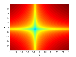
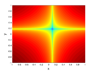
Figure 1: Two different experiments representing contours of $MS_{p}$ for $p=0.1$ and $\tau=15$. The contours of $MS_{p}$ are computed on a 1200$\times$ 1200 points grid of initial conditions and the time step for integration of the vector field is chosen to be $\Delta t=0.05$. The magenta colored point corresponds to the location of the stationary orbit for each experiment. The chosen parameters are $a_{1}=a_{2}=b_{2}=1$ and $b_{1}=-1$.

Remark 5.1.

Due to the properties of Itô integrals, see for instance duan15 , the components of the stationary orbit satisfy

$$\mathbb{E}\left[\tilde{x}(\omega)\right]=\mathbb{E}\left[-\int_{0}^{\infty}e^{-s}dW_{s}^{1}\right]=0\quad,\quad\mathbb{E}\left[\tilde{y}(\omega)\right]=\mathbb{E}\left[\int_{-\infty}^{0}e^{s}dW_{s}^{2}\right]=0,$$

$$\mathbb{V}\left[\tilde{x}(\omega)\right]=\mathbb{E}\left[\tilde{x}(\omega)^{2}\right]=\mathbb{E}\left[\int_{0}^{\infty}e^{-2s}ds\right]=\frac{1}{2}\quad,\quad\mathbb{V}\left[\tilde{y}(\omega)\right]=\mathbb{E}\left[\tilde{y}(\omega)^{2}\right]=\mathbb{E}\left[\int_{-\infty}^{0}e^{2s}ds\right]=\frac{1}{2}.$$

This means that the stationary orbit $(\tilde{x}(\omega),\tilde{y}(\omega))$ is highly probable to be located closed to the origin of coordinates $(0,0)$, and this feature is displayed in Figure 1. This result gives more evidences and supports the similarities between the stochastic differential equation (5) and the deterministic analogue system $\{\dot{x}=x,\hskip 2.84544pt\dot{y}=-y\}$ whose only fixed point is $(0,0)$.

Therefore we can assert that the stochastic Lagrangian descriptor is a technique that provides a phase portrait representation of the dynamics generated by the noisy saddle equation (27). Next we apply this same technique to further examples.

6 Other examples

6.1 Stochastically forced Duffing equation

Another classical problem is the Duffing oscillator. The deterministic version is given by

$$\ddot{x}=\alpha\dot{x}+\beta x+\gamma x^{3}+\epsilon\cos(t).$$ (35)

If $\epsilon=0$ the Duffing equation becomes time-independent, meanwhile for $\epsilon\neq 0$ the oscillator is a time-dependent system, where $\alpha$ is the damping parameter, $\beta$ controls the rigidity of the system and $\gamma$ controls the size of the nonlinearity of the restoring force. The stochastically forced Duffing equation is studied in datta01 and can be written as follows:

$$\begin{cases}dX_{t}=\alpha Y_{t},\\ dY_{t}=(\beta X_{t}+\gamma X^{3}_{t})dt+\epsilon dW_{t}.\end{cases}$$ (36)

For our numerical experiments we have selected $\alpha=\beta=1$, $\gamma=-1$ and $\epsilon=0.25$. The results of three different experiments (let say three different samples of $\omega_{1},\omega_{2},\omega_{3}\in\Omega$) are shown in Figure 2.

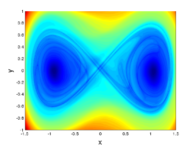
(a) $MS_{p}$ contours for $\omega_{1}$

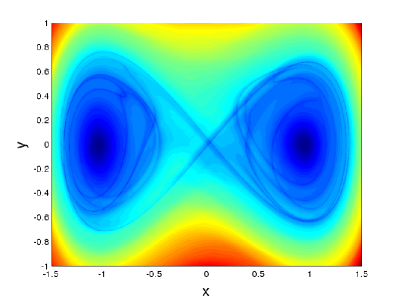
(b) $MS_{p}$ contours for $\omega_{2}$

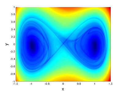
(c) $MS_{p}$ contours for $\omega_{3}$

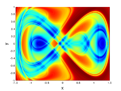
(d) $M_{p}$ for equation $\eqref{eq:duffing_determ}$

Figure 2: a), b), c) Three different experiments representing $MS_{p}$ contours for $p=0.5$ over a grid of initial conditions. d) The last image corresponds to the $M_{p}$ function for equation (35) and $p=0.75$. All these pictures were computed for $\tau=15$, and over a $1200\times 1200$ points grid. The time step for integration of the vector field was chosen to be $\Delta t=0.05$.

6.2 Stochastically forced Double Gyre

The double gyre is a standard benchmark velocity field in the study of the dynamical systems approach to Lagrangian transport. Recently it has been studied in the situation where the time-dependence is stochastic (hsieh12 ). These equations are given by

$$\begin{cases}dX_{t}=\displaystyle{\left(-\pi A\sin\Big{(}\pi\frac{f(X_{t},t)}{s}\Big{)}\cos\Big{(}\pi\frac{Y_{t}}{s}\Big{)}-\mu X_{t}\right)dt+\alpha dW^{1}_{t}},\\ \\ dY_{t}=\displaystyle{\left(\pi A\cos\Big{(}\pi\frac{f(X_{t},t)}{s}\Big{)}\sin\Big{(}\pi\frac{Y_{t}}{s}\Big{)}\frac{\partial f}{\partial X_{t}}-\mu Y_{t}\right)dt+\alpha dW^{2}_{t}},\end{cases}$$ (37)

where

$$f(X_{t},t)=\epsilon\sin(\phi t+\psi)X_{t}^{2}+(1-2\epsilon\sin(\phi t+\psi))X_{t}.$$ (38)

When $\epsilon=0$ the double-gyre is time-independent, meanwhile if $\epsilon\neq 0$ the gyres force a periodic behavior in the $x$ direction. Among the parameters within the equation, $A$ models the amplitude of the velocity vectors, $\frac{\phi}{2\pi}$ gives the oscillation frequency, $\psi$ is the phase, $\mu$ determines the dissipation, $s$ scales the dimensions of the grid and $dW^{i}_{t}$ describes a Wiener process (stochastic white noise) with mean zero and standard deviation $\sigma=\Delta t$, while $\alpha$ is the amplitude of the noise. The results of two different experiments are observed in Figure 3. For such experiments we have used the following values for the parameters: $A=0.25$, $\phi=2\pi$, $\psi=0$, $\mu=0$, $s=1$, $\alpha=0.1$, $\epsilon=0.25$.

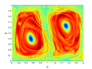
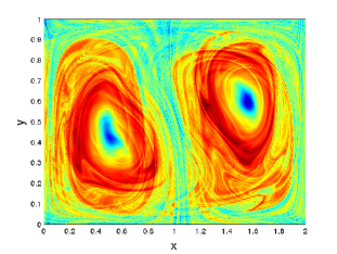
Figure 3: Two different experiments representing contours of $MS_{p}$ for $p=0.5$ and $\tau=15$. The contours of $MS_{p}$ are computed on a $1200\times 1200$ points grid of initial conditions and the time step for integration of the vector field is chosen to be $\Delta t=0.05$.

The outputs are quite different between these two experiments. Therefore we make use of (23). In Figure 4 we can observe the values of $\mathbb{E}\left[MSp\right]$ when considering 30 different experiments. This is the expected phase space structure: two gyre centers are detected near the points $(0.5,0.5)$ and $(1.5,0.5)$ in dark blue, while around the line $\{x=1\}$ we observe bundles of invariant manifolds in light blue. Thus for almost every $\omega\in\Omega$ two centers are depicted close to the middle of each gyre and by separating each gyre, the invariant manifolds can be interpreted as transport barriers.

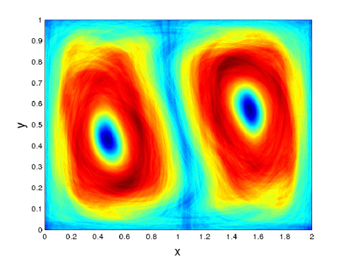
Figure 4: Computation of $\mathbb{E}\left[MS_{p}(\cdot,\omega)\right]$ for $p=0.5$, $\tau=15$ and 30 different experiments with a time step integration $\Delta t=0.05$.

In order to clarify the structures highlighted in Figure 4, we select a point in the middle of the gyre, the point $(0.5,0.425)$, and we evolve it forwards and backwards in time for different realizations of the random variable $\omega$. In Figure 5 there are represented different snapshots for several units of time. As the random dynamical system evolves, the different trajectories starting at the point $(0.5,0.425)$ remain bounded inside the gyre. Only when the system evolves for a enough period of time, it is observable that hyperbolicity affects most of the trajectories.

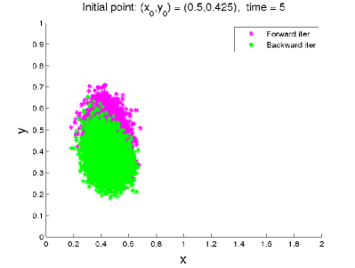
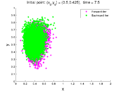
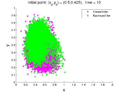
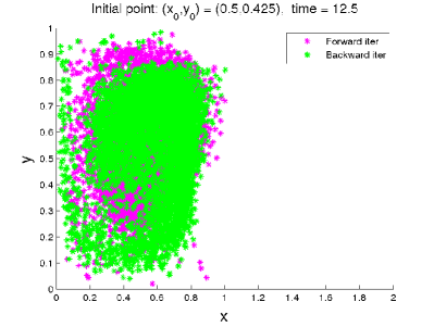
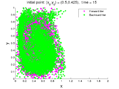
Figure 5: 5000 distinct simulations of trajectories starting at the point $(0.5,0.425)$ and performed forwards and backwards for several intervals of time.

Furthermore, in order to verify the shape that the invariant manifolds take, the point $(1,0.5)$ is evolved forward and backward in time for different realizations of the random variable $\omega$. In Figure 6 we overlap 5000 different trajectories starting at the same point with the expected phase space shown in the background and examine how these trajectories fit the sharp lines corresponding to the already computed invariant manifolds.

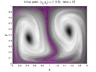
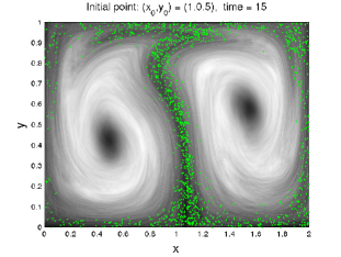
Figure 6: Representation of the ending points of 5000 distinct trajectories iterated in forward time from $t=0$ until $t=15$ (left hand panel, in magenta dots) and the ending points of 5000 distinct trajectories iterated in backward time from $t=0$ until $t=-15$ (right hand panel, in green dots). All these trajectories start at the same initial point $(x_{0},y_{0})=(1,0.5)$ but their respective evolutions are influenced by different Wiener processes. In addition, $\mathbb{E}\left[MS_{p}(\cdot,\omega)\right]$ is computed for the time periods $[-\tau,0]$ and $[0,\tau]$. These expected phase spaces are depicted in the background of the left and right hand panels respectively with $p=0.5$ for 30 different experiments.

These pictures provide evidence for the strong correspondance between the paths followed by the particles and the structures depicted in bluish colours in Figure 4. Notice that in this last Figure 6, the mean $\mathbb{E}\left[MS_{p}(\cdot,\omega)\right]$ computed for the time period $[-\tau,\tau]$ and represented in Figure 4 has been split into two quantities. From the deterministic Lagrangian descriptors setting (see LBGWM15 ), the trajectories iterated in forward time and starting in a neighborhood of a hyperbolic point approximate the location of the unstable manifold for a large integration time $\tau$. Similarly, the trajectories iterated in backward time follow the path of the stable manifold in a neighborhood of the hyperbolic point. In summary, these simulations support the idea of the method of stochastic Lagrangian descriptors as useful for depicting areas where the hyperbolic trajectories with their stable and unstable manifolds are likely located.

7 Summary and Conclusions

In this paper we have extended the method of Lagrangian descriptors to stochastic differential equations (SDEs). We have shown that the resulting method provides a way of revealing the global phase space structure of SDEs that is analogous the the manner in which we understand the global phase space structure of deterministic ordinary differential equations. In particular, we show that stochastic versions of hyperbolic trajectories and their stable and unstable manifolds provide barriers to transport. We apply our method to the noisy saddle, the stochastically forced Duffing equation, and the stochastic double gyre model that is a benchmark for analyzing fluid transport.

Appendix 1. Deterministic solution mappings

Taking as a reference the book by Kloeden and Rasmussen (kloe11 ), the solution mappings will be defined over a temporal domain $\mathbb{T}$, which is usually taken to be $\mathbb{R}$ (continuous time), and over a spatial domain $X$ which is usually taken to be $\mathbb{R}^{n}$. In both the autonomous and the nonautonomous settings, the solution mappings are denoted by $\phi$, and these clearly correspond to the solutions of some given deterministic differential equations.

For an autonomous differential equation $\dot{x}=f(x)$, the solution mapping $\phi$ is usually referred to as a flow, less often it is referred to as dynamical system, and it depends only on two variables: the evolution variable $t$ and the initial condition $x_{0}$, although $\phi$ might not be defined over the entire temporal and spatial domains $\mathbb{T}$ and $X$. For any fixed initial condition $x_{0}\in X$, the mapping $\phi(\cdot,x_{0})$ is a solution of the differential equation. Formally it satisfies the properties.

Definition 7.1.

A dynamical system is a continuous function $\phi\mathrel{\mathop{\mathchar 58\relax}}\mathbb{T}\times X\rightarrow X$ which satisfies the following two properties,

1. Initial value condition. $\phi(0,x_{0})=x_{0}$ for all $x_{0}\in X$,

2. Group property. $\phi(s+t,x_{0})=\phi(s,\phi(t,x_{0}))$ for all $s,t\in\mathbb{T}$ and $x_{0}\in X$.

The solution mappings for nonautonomous differential equations of the kind $\dot{x}=f(x,t)$ are known as processes, and share many similarities with dynamical systems in the autonomous case. The main difference is that $\phi$ depends on an extra variable, the initial time $t_{0}$ when the solution $x(t)$ of the differential equation passes through $x_{0}$, let say $x(t_{0})=x_{0}$. This is due to the time-dependence of the vector field field $f(x,t)$.

Definition 7.2.

A process is a continuous mapping $(t,t_{0},x_{0})\mapsto\phi(t,t_{0},x_{0})\in X$ for $t,t_{0}\in\mathbb{T}$ and $x_{0}\in X$, which satisfies the initial value and evolution properties,

1. $\phi(t_{0},t_{0},x_{0})=x_{0}$ for all $t_{0}\in\mathbb{T}$ and $x_{0}\in X$,

2. $\phi(t_{2},t_{0},x_{0})=\phi(t_{2},t_{1},\phi(t_{1},t_{0},x_{0}))$ for all $t_{0},t_{1},t_{2}\in\mathbb{T}$ and $x_{0}\in X$.

Appendix 2. RDSs for time-dependent SDEs

As mentioned in Section 2, just after the introduction of the formal definition of random dynamical system, this was only appropriate for SDEs with time-independent coefficients $b,\sigma$. Inspired in this Definition 2.2 given by J. Duan (duan15 ), we develop the same notion of RDS for a more general context, where at least $b$ or $\sigma$ do depend explicitly on the time variable $t$. For this purpose it is necessary to consider a fourth argument for the solution mapping $\varphi$, which is the initial time $t_{0}$ when $\varphi$ passes through the initial condition $x_{0}$. This has been done in the same way that processes are built from flow mappings in the deterministic differential equations setting.

Definition 7.3.

Let $\{\theta_{t}\}_{t\in\mathbb{R}}$ be a measure-preserving dynamical system defined over $\Omega$, and let $\varphi\mathrel{\mathop{\mathchar 58\relax}}\mathbb{R}\times\mathbb{R}\times\Omega\times\mathbb{R}^{n}\rightarrow\mathbb{R}^{n}$ be a measurable mapping such that $(t,t_{0},\cdot,x)\mapsto\varphi(t,t_{0},\omega,x)$ is continuous for all $\omega\in\Omega$, and the family of functions $\{\varphi(t,t_{0},\omega,\cdot)\mathrel{\mathop{\mathchar 58\relax}}\mathbb{R}^{n}\rightarrow\mathbb{R}^{n}\}$ has the cocycle property,

$$\varphi(t_{0},t_{0},\omega,x)=x\quad\text{and}$$

$$\varphi(t_{2},t_{0},\omega,x)=\varphi(t_{2},t_{1},\theta_{(t_{1}-t_{0})}\omega,\varphi(t_{1},t_{0},\omega,x))\quad\text{for all }t_{0},t_{1},t_{2}\in\mathbb{R},\text{ }x\in\mathbb{R}^{n}\text{ and }\omega\in\Omega.$$

Then the mapping $\varphi$ is a random dynamical system with respect to the stochastic differential equation

$$dX_{t}=b(X_{t},t)dt+\sigma(X_{t},t)dW_{t}$$

if $\varphi(t,t_{0},\omega,x)$ is a solution of the equation.

Appendix 3. Multiplicative Ergodic Theorem

The next results are taken from the book by J. Duan (2015) (duan15 ). These are essential in order to understand the hyperbolicity of a given stationary orbit $\tilde{X}(\omega)$ with respect to a random dynamical system $\varphi$.

We begin by centering $\varphi$ at $\tilde{X}(\omega)$, therefore achieving a new RDS,

$$\widetilde{\varphi}(t,\omega,x)=\varphi(t,\omega,\tilde{X}(\omega)+x)-\tilde{X}(\theta_{t}\omega).$$

This mapping $\widetilde{\varphi}$ retains the same dynamics as $\varphi$, with the difference that the constant value trajectory $X\equiv 0$ is a random fixed point for $\widetilde{\varphi}$. Now $\widetilde{\varphi}$ linearized with respect to the initial condition variable $x\in\mathbb{R}^{n}$ and evaluated at the initial condition $x=0$,

$$\Phi(t,\omega)=\frac{\partial}{\partial x}\widetilde{\varphi}(t,\omega,x=0)=\frac{\partial}{\partial x}\varphi(t,\omega,x=\tilde{X}(\omega))$$

allows us to conveniently study whether or not $\tilde{X}(\omega)$ is hyperbolic by applying the following theorem.

Theorem 7.4.

Multiplicative ergodic theorem (MET). Let $\Phi(t,\omega)$ be a linear RDS (linear cocycle) in $\mathbb{R}^{n}$, for $t\in\mathbb{R}$, on a probability space $(\Omega,\mathcal{F},\mathcal{P})$, over a measurable driving flow $\theta_{t}$. Assume that the following integrability conditions are satisfied:

$${\sup_{0\leq t\leq 1}\ln^{+}\mathinner{\!\left\lVert\Phi(t,\omega)\right\rVert}\in L^{1}(\Omega),\quad\sup_{0\leq t\leq 1}\ln^{+}\mathinner{\!\left\lVert\Phi(-t,\omega)\right\rVert}\in L^{1}(\Omega),}$$ (39)

where $\ln^{+}(z)\mathrel{\mathop{\mathchar 58\relax}}=\max\{\ln(z),0\}$, denoting the nonnegative part of the natural logarithm. Then there exists an invariant set $\widetilde{\Omega}\in\mathcal{F}$ of full probability measure, such that for every $\omega\in\widetilde{\Omega}$,

1. the asymptotic geometric mean $\lim_{t\to\pm\infty}[\Phi(t,\omega)^{T}\Phi(t,\omega)]^{\frac{1}{2t}}=\widetilde{\Phi}$ exists and it is nonnegative definite $n\times n$ matrix.

2. the matrix $\widetilde{\Phi}$ has distinct eigenvalues $e^{\lambda_{p}(\omega)}<\cdots,e^{\lambda_{1}(\omega)},\omega\in\widetilde{\Omega}$, with corresponding eigenspaces $E_{p(\omega)}(\omega),\cdots,E_{1}(\omega)$ of dimensions $d_{i}(\omega)=\dim E_{i}(\omega),i=1,\cdots,p(\omega)$. These eigenspaces are such that $E_{1}(\omega)\oplus E_{2}(\omega)\oplus\cdots\oplus E_{p(\omega)}(\omega)=\mathbb{R}^{n}$. Moreover, $p$, $\lambda_{i}$ and $d_{i}$ are invariant under the driving flow $\theta_{t}$ in the following sense:

   $$p(\theta_{t}\omega)=p(\omega),\quad\lambda_{i}(\theta_{t}\omega)=\lambda_{i}(\omega)\quad\text{ and }\quad d_{i}(\theta_{t}\omega)=d_{i}(\omega)$$

   for $i=1,\cdots,p,t\in\mathbb{R}$ and $\omega\in\widetilde{\Omega}$.

3. each $E_{i}(\omega)$ is invariant for the linear RDS: $\Phi(t,\omega)E_{i}(\omega)=E_{i}(\theta_{t}\omega)$, for all $\omega\in\widetilde{\Omega}$ and all $t\in\mathbb{R}$.

4. $\lim_{t\to\pm\infty}1/t\ln\mathinner{\!\left\lVert\Phi(t,\omega)x\right\rVert}=\lambda_{i}$ if and only if $x\in E_{i}(\omega)-\{0\}$, for all $\omega\in\widetilde{\Omega}$ and $i=1,\cdots,p$.

Definition 7.5.

Let $\Phi(t,\omega)$ be a linear RDS in $\mathbb{R}^{n}$ that satisfies the initial conditions of the MET. The vector subspaces based on the Oseledets spaces

$$E^{s}(\omega)=\bigoplus_{\lambda_{i}<0}E_{i}(\omega)\quad,\quad E^{c}(\omega)=\bigoplus_{\lambda_{i}=0}E_{i}(\omega)\quad,\quad E^{u}(\omega)=\bigoplus_{\lambda_{i}>0}E_{i}(\omega)$$

are called the stable, center and unstable subspaces of $\Phi(t,\omega)$, respectively. The family of its Lyapunov exponents and their corresponding multiplicities

$$\{\lambda_{1},\cdots,\lambda_{p};d_{1},\cdots,d_{p}\}$$

is called the Lyapunov spectrum of $\Phi(t,\omega)$. Moreover if all the Lyapunov exponents are nonzero then the linear RDS $\Phi(t,\omega)$ is said to be hyperbolic.

As mentioned before in Section 2, the random dynamical system (7) associated to the noisy saddle (5) satisfies the conditions of the Multiplicative ergodic theorem. This fact and the simplicity of the noisy saddle, allows us to compute explicitly the Lyapunov spectrum and the stable and unstable subspaces of the RDS $\Phi(t,\omega)$ linearized over the stationary orbit $\tilde{X}(\omega)$.

Example 7.6.

(Noisy saddle point)

The random dynamical system $\varphi$ corresponding to the noisy saddle (5) has the expression,

$$\begin{array}[]{ccccccccc}\varphi\mathrel{\mathop{\mathchar 58\relax}}&&\mathbb{R}\times\Omega\times\mathbb{R}^{2}&&\longrightarrow&&\mathbb{R}^{2}&&\\ &&(t,\omega,(x,y))&&\longmapsto&&\left(\varphi_{1}(t,\omega,x),\varphi_{2}(t,\omega,y)\right)&=&\left(e^{t}\left(x+\int_{0}^{t}e^{-s}dW_{s}^{1}(\omega)\right),e^{-t}\left(y+\int_{0}^{t}e^{s}dW_{s}^{2}(\omega)\right)\right).\end{array}$$

The Jacobian matrix $D_{(x,y)}\varphi$ does not depend on the third argument, let say the initial condition $(x,y)$,

$$\Phi(t)=D_{(x,y)}\varphi(t,\omega,(x,y))=\left(\begin{array}[]{cc}e^{t}&0\\ 0&e^{-t}\end{array}\right).$$

As this linear cocycle is a diagonal matrix, its norm corresponds to the largest element of its diagonal, which is also the largest eigenvalue. In this case,

$$||\Phi(t)||=||\Phi(-t)||=\begin{cases}e^{t}\quad\text{for }t\geq 0\\ e^{-t}\quad\text{for }t<0\end{cases}\text{and}\quad\displaystyle{\sup_{0\leq t\leq 1}\ln^{+}\mathinner{\!\left\lVert\Phi(t)\right\rVert}}=\displaystyle{\sup_{0\leq t\leq 1}\ln^{+}\mathinner{\!\left\lVert\Phi(-t)\right\rVert}}=\displaystyle{\sup_{0\leq t\leq 1}|t|}=1.$$

As any constant function belongs to the space of functions $L^{1}(\Omega)$ (remember that the probability space $\Omega$ has measure equal to 1), the conditions of the MET are satisfied. Now for the asymptotic geometric mean,

$$\widetilde{\Phi}=\lim_{t\to\pm\infty}[\Phi(t)^{T}\Phi(t)]^{\frac{1}{2t}}=\left[\left(\begin{array}[]{cc}e^{t}&0\\ 0&e^{-t}\end{array}\right)\cdot\left(\begin{array}[]{cc}e^{t}&0\\ 0&e^{-t}\end{array}\right)\right]^{\frac{1}{2t}}=\left(\begin{array}[]{cc}e^{2t}&0\\ 0&e^{-2t}\end{array}\right)^{\frac{1}{2t}}=\left(\begin{array}[]{cc}e^{1}&0\\ 0&e^{-1}\end{array}\right),$$

its associated eigenvalues are $e^{1}$ and $e^{-1}$, with corresponding eigenspaces $\text{span}\{\left(\begin{array}[]{c}1\\ 0\end{array}\right)\}$ and $\text{span}\{\left(\begin{array}[]{c}0\\ 1\end{array}\right)\}$ respectively. These two linear subspaces are precisely the unstable $E^{u}(\omega)$ and the stable $E^{s}(\omega)$ subspaces of $\Phi(t)$, for which the Lyapunov spectrum is $\{\lambda_{1}=1,\lambda_{2}=-1\}$, therefore confirming the hyperbolic nature of the stationary orbit. It results evident that for any other more complex SDE, the computation of the asymptotic geometric mean $\tilde{\Phi}$ would be more tricky; highlighting that this process is not straightforward for most SDEs.

What remains is to establish the relationship between the linear subspaces $E^{u}(\omega)$, $E^{s}(\omega)$ and the already mentioned $\mathcal{U}(\omega)$, $\mathcal{S}(\omega)$. This is discussed in Theorem 3.1 from Mohammed and Scheutzow (moham99 ) where the local unstable and the local stable manifolds of a stationary orbit $\tilde{X}(\omega)$ are related to the sets of points (in a neighborhood of $\tilde{X}(\omega)$) which are attracted by the stationary orbit in negative or positive time, respectively. In summary this fact presents many similarities with the definition of exponential dichotomy for deterministic dynamical systems. Indeed this exponentially attracting rate over the points of the manifolds $\mathcal{U}(\omega)$, $\mathcal{S}(\omega)$ of the noisy saddle (5) is easily observed in Equation (12),

$$(\overline{x}_{t},\overline{y}_{t})-(\tilde{x}(\theta_{t}\omega),\tilde{y}(\theta_{t}\omega))=\varphi(t,\omega,(\overline{x}_{0},\overline{y}_{0}))-\varphi(t,\omega,(\tilde{x}(\omega),\tilde{y}(\omega)))=\left(\epsilon_{1}(\omega)e^{t},\epsilon_{2}(\omega)e^{-t}\right),$$

regardless the initial distance $\left(\epsilon_{1}(\omega),\epsilon_{2}(\omega)\right)$ of $(\bar{x_{t}},\bar{y_{t}})$ to the stationary orbit $\tilde{X}(\omega)$. Moreover, as this distance can be arbitrarily large, the dynamics in a neighborhood of $\tilde{X}(\omega)$ are also achieved for the rest of trajectories within the invariant sets $\mathcal{U}(\omega)$, $\mathcal{S}(\omega)$, giving to these a global property. This argument enables us to simply refer to $\mathcal{U}(\omega)$ and $\mathcal{S}(\omega)$ as the unstable and stable manifolds of the stationary orbit of the noisy saddle equation (5).

References

- [1] L. Arnold. Random Dynamical Systems. Springer, 1998.
- [2] R. Banisch and P. Koltai. Understanding the geometry of transport: diffusion maps for Lagrangian trajectory data unravel coherent sets. http://arxiv.org/abs/1603.04709, 2016.
- [3] P. Boxler. A Stochastic Version of Center Manifold Theory. Probability Theory and Related Fields, 83:509–545, 1989.
- [4] Z. Cheng, J. Duan, and L. Wang. Most probable dynamics of some nonlinear systems under noisy fluctuations. Commun. Nonlinear Sci. Numer. Simulat., 30(1):108–114, 2016.
- [5] G. T. Craven and R. Hernandez. Lagrangian descriptors of thermalized transition states on time-varying energy surfaces. Phys. Rev. Lett., 115:148301, 2015.
- [6] G. T. Craven and R. Hernandez. Deconstructing field-induced ketene isomerization through Lagrangian descriptors. Phys. Chem. Chem. Phys., 18:4008, 2016.
- [7] S. Datta and J. K. Bhattacharjee. Effect of stochastic forcing on the Duffing oscillator. Physics Letters A, 283:323–326, 2001.
- [8] A. de la Cámara, A. M. Mancho, K. Ide, E. Serrano, and C.R. Mechoso. Routes of transport across the Antarctic polar vortex in the southern spring. J. Atmos. Sci., 69(2):753–767, 2012.
- [9] A. de la Cámara, C. R. Mechoso, E. Serrano, and K. Ide. Quasi-horizontal transport within the Antarctic polar night vortex: Rossby wave breaking evidence and Lagrangian structures. J. Atmos. Sci., 70:2982–3001, 2013.
- [10] J. Duan. An Introduction to Stochastic Dynamics. Cambridge University Press, 2015.
- [11] V. J. García-Garrido, A. M. Mancho, S. Wiggins, and C. Mendoza. A dynamical systems approach to the surface search for debris associated with the disappearance of flight MH370. Nonlin. Proc. Geophys., 22:701–712, 2015.
- [12] V. J. García-Garrido, A. Ramos, A. M. Mancho, J. Coca, and S. Wiggins. A dynamical systems perspective for a real-time response to a marine oil spill. submitted to Marine Pollution Bulletin, 2016.
- [13] M.A. Hsieh, E. Forgoston, T. W. Mather, and I.B. Schwartz. Robotic manifold tracking of coherent structures in flows Robotics and Automation. Robotics, IEEE International Conference, 30:593–603, 2012.
- [14] K. Ide, D. Small, and S. Wiggins. Distinguished hyperbolic trajectories in time dependent fluid flows: analytical and computational approach for velocity fields defined as data sets. Nonlin. Proc. Geophys., 9:237–263, 2002.
- [15] A. Junginger and R. Hernandez. Lagrangian descriptors in dissipative systems. Phys. Chem. Chem. Phys., 2016.
- [16] A. Junginger and R. Hernandez. Uncovering the geometry of barrierless reactions using Lagrangian descriptors. J. Phys. Chem. B, 2016.
- [17] P. E. Kloeden and E. Platen. Numerical Solution of Stochastic Differential Equations. Applications of Mathematics 23. Springer-Verlag Berlin Heidelberg, 1 edition, 1992.
- [18] P. E. Kloeden and M. Rasmussen. Nonautonomous Dynamical Systems, volume 176 of Mathematical Surveys and Monographs. American Mathematical Society, Providence, Rhode Island, 2011.
- [19] C. Lopesino, F. Balibrea, S. Wiggins, and A. M. Mancho. Lagrangian Descriptors for Two Dimensional, Area Preserving Autonomous and Nonautonomous Maps. Communications in Nonlinear Science and Numerical Simulation, 27(1-3):40–51, 2015.
- [20] C. Lopesino, F. Balibrea-Iniesta, V. J. García-Garrido, S. Wiggins, and A. M. Mancho. A theoretical framework for Lagrangian descriptors. submitted to Comm. Nonlin. Sci. Numer. Simul., 2016.
- [21] J. A. J. Madrid and A. M. Mancho. Distinguished trajectories in time dependent vector fields. Chaos, 19:013111, 2009.
- [22] A. M. Mancho, J. Curbelo, S. Wiggins, V. J. García-Garrido, and C. Mendoza. Beautiful Geometries Underlying Ocean Nonlinear Processes, pages 80–85. European Geophysical Union, 2015.
- [23] A. M. Mancho, S. Wiggins, J. Curbelo, and C. Mendoza. Lagrangian Descriptors: A Method for Revealing Phase Space Structures of General Time Dependent Dynamical Systems. Communications in Nonlinear Science and Numerical Simulation, 18:3530–3557, 2013.
- [24] C. Mendoza and A. M. Mancho. The hidden geometry of ocean flows. Phys. Rev. Lett., 105(3):038501, 2010.
- [25] C. Mendoza and A. M. Mancho. The Lagrangian description of ocean flows: a case study of the Kuroshio current. Nonlin. Proc. Geophys., 19(4):449–472, 2012.
- [26] C. Mendoza, A. M. Mancho, and S. Wiggins. Lagrangian Descriptors and the Assesment of the Predictive Capacity of Oceanic Data Sets. Nonlin. Proc. Geophys., 21:677–689, 2014.
- [27] S.-E. A. Mohammed and M. K. R. Scheutzow. The Stable Manifold Theorem for Stochastic Differential Equations. Ann. Probab., 27(2):615–652, 1999.
- [28] E. L. Rempel, A. C.-L. Chian, A. Brandenburg, P. R. Munuz, and S. C. Shadden. Coherent structures and the saturation of a nonlinear dynamo. Journal of Fluid Mechanics, 729:309–329, 2013.