THE CHAOTIC SADDLE IN THE LOZI MAP, AUTONOMOUS AND NONAUTONOMOUS VERSIONS

Abstract

In this paper we prove the existence of a chaotic saddle for a piecewise linear map of the plane, referred to as the Lozi map. We study the Lozi map in its orientation and area preserving version. First, we consider the autonomous version of the Lozi map to which we apply the Conley-Moser conditions to obtain the proof of a chaotic saddle. Then we generalize the Lozi map on a non-autonomous version and we prove that the first and the third Conley-Moser conditions are satisfied, which imply the existence of a chaotic saddle. Finally, we numerically demonstrate how the structure of this nonautonomous chaotic saddle varies as parameters are varied.

1 Introduction

In this paper we prove that the Lozi map (Lozi [1978]), as well as a nonautonomous generalization of the Lozi map, possesses a chaotic saddle, i.e. a hyperbolic invariant set on which the dynamics is topologically conjugate to a Bernoulli shift. Our construction uses the Conley-Moser conditions for autonomous maps as developed in Moser [1973] (see also Wiggins [2003]) and the nonautonomous Conley-Moser conditions as developed in Wiggins [1999] and Balibrea-Iniesta, et al. [2015]. For earlier work in a similar spirit as the Conley-Moser conditions see Alekseev [1968a, b, 1969].

Previously, the autonomous Conley-Moser conditions have been used by Devaney and Nitecki [1979] to show the existence of a chaotic invariant set for the Hénon map and by Holmes [1982] and Chastaing, et al. [2014] to show the existence of a chaotic invariant set for the bouncing ball map.

While the development of the “dynamical systems approach to nonautonomous dynamics” is currently a topic of much interest in the pure mathematics community, it is not a topic that is widely known in the applied dynamical systems community (especially the fundamental work that was done in the 1960’s). An applied motivation for such work is an understanding from the dynamical systems point of view of fluid transport for aperiodically time dependent flows. Wiggins and Mancho [2014] have given a survey of the history of nonautonomous dynamics as well as its application to fluid transport. Earlier work on chaos in nonautonomous systems is described in Lerman and Silnikov [1992]; Stoffer [1988a, b].

This paper is outlined as follows. In section 1 we introduce the setup of the problem. The definitions and theorems given in this section make clear what we mean by the phrase “ chaotic invariant set ” for both autonomous and nonautonomous maps. In sections 3 and 4 we construct chaotic invariant sets (i.e., chaotic saddles) for both the autonomous and nonautonomous versions of the Lozi map, respectively. In section 5 we show how these sets are detected using the Discrete Lagrangian Descriptor (see Lopesino, et al. [2015]) for different parameter values, both in the autonomous or in the nonautonomous case. Finally, in section 6 we summarize our results.

2 Setup and geometry of the problem

In this section we recall the set-up for the autonomous Conley-Moser conditions that were introduced by Moser [1973] and the nonautonomous Conley-Moser conditions introduced in Wiggins [1999]. We follow the structure in Wiggins [2003] for our exposition, but with an inverse notation (that is $f\equiv L^{-1}$ in the autonomous case and $f_{n}\equiv L_{n}^{-1}$ in the nonautonomous case, where we use the notation $L$ in the autonomous case and $L_{n}^{-1}$ in the nonautonomous case to denote the general form for the maps under consideration, rather than $f$ and $f_{n}$, respectively, from the original references, since $L$ is traditionally used to refer to the Lozi map).

2.1 The Autonomous Conley-Moser Conditions

We begin with the following two definitions.

Definition 2.1.

A $\mu_{v}$-vertical curve is the graph of a function $x=v(y)$ for which

$$-R\leq v(y)\leq R,\qquad|v(y_{1})-v(y_{2})|\leq\mu_{v}|y_{1}-y_{2}|\quad\text{for }-R\leq y_{1},y_{2}\leq R.$$

Similarly, a $\mu_{h}$-horizontal curve is the graph of a function $y=h(x)$ for which

$$-R\leq h(x)\leq R,\qquad|h(x_{1})-h(x_{2})|\leq\mu_{h}|x_{1}-x_{2}|\quad\text{for }-R\leq x_{1},x_{2}\leq R.$$

Definition 2.2.

Given two nonintersecting $\mu_{v}$-vertical curves $v_{1}(y)<v_{2}(y)$, $y\in[-R,R]$, we define a $\mu_{v}$-vertical strip as

$$V=\left\{(x,y)\in\mathbb{R}^{2}|x\in[v_{1}(y),v_{2}(y)];\quad y\in[-R,R]\right\}.$$

Similarly, given two nonintersecting $\mu_{h}$-horizontal curves $h_{1}(x)<h_{2}(x)$, $x\in[-R,R]$, we define a $\mu_{h}$-horizontal strip as

$$H=\left\{(x,y)\in\mathbb{R}^{2}|y\in[h_{1}(x),h_{2}(x)];\quad x\in[-R,R]\right\}.$$

The width of horizontal and vertical strips is defined as

$$d(H)=\max_{x\in[-R,R]}|h_{2}(x)-h_{1}(x)|,$$

$$d(V)=\max_{y\in[-R,R]}|v_{2}(y)-v_{1}(y)|.$$

Keeping these definitions in mind, we begin with the Conley Moser conditions for the autonomous case. We consider a map

$$L:D\longrightarrow\mathbb{R}^{2},$$

where $D$ is a square in $\mathbb{R}^{2}$, i.e.,

$$D=\left\{(x,y)\in\mathbb{R}^{2}|-R\leq x\leq R,\quad-R\leq y\leq R\right\}.$$

Let

$$I=\left\{1,2,...,N\right\},\qquad(N\geq 2),$$

be an index set, and let

$$H_{i},\qquad i\in I$$

be a set of disjoint $\mu_{h}$-horizontal strips and let

$$V_{i},\qquad i\in I$$

be a set of disjoint $\mu_{v}$-vertical strips. Suppose that $L$ satisfies the following two conditions.

Assumption 1: $0\leq\mu_{v}\mu_{h}<1$ and $L$ maps $V_{i}$ homeomorphically onto $H_{i}$, ($L(V_{i})=H_{i}$) for $i\in I$. Moreover, the horizontal boundaries of $V_{i}$ map to the horizontal boundaries of $H_{i}$ and the vertical boundaries of $V_{i}$ map to the vertical boundaries of $H_{i}$.

Assumption 2: Suppose $H$ is a $\mu_{h}$-horizontal strip contained in $\cup_{i\in I}H_{i}$. Then

$$L(H)\cup H_{i}\equiv\tilde{H}_{i}$$

is a $\mu_{h}$-horizontal strip for every $i\in I$. Moreover,

$$d(\tilde{H}_{i})\leq\nu_{h}d(H)\qquad\text{for some}\quad 0<\nu_{h}<1.$$

Similarly, suppose $V$ is a $\mu_{v}$-vertical strip contained in $\cup_{i\in I}V_{i}$. Then

$$L^{-1}(V)\cap V_{i}\equiv\tilde{V}_{i}$$

is a $\mu_{v}$-vertical strip for every $i\in I$. Moreover,

$$d(\tilde{V}_{i})\leq\nu_{v}d(V)\qquad\text{for some}\quad 0<\nu_{v}<1.$$

Then we have the following theorem.

Theorem 2.3.

Suppose $L$ satisfies Assumptions $1$ and $2$. Then $L$ has an invariant Cantor set, $\Lambda$, on which it is topologically conjugate to a full shift on $N$ symbols, i.e., the following diagram commutes

$$\begin{array}[]{ccccc}&&L&&\\ &\Lambda&\longrightarrow&\Lambda\\ \\ \phi&\downarrow&&\downarrow&\phi\\ &&\sigma&&\\ &\Sigma^{N}&\longrightarrow&\Sigma^{N}&\\ \end{array}$$ (1)

where $\phi$ is a homeomorphism mapping $\Lambda$ onto $\Sigma^{N}$ and $\sigma$ denotes the shift map acting on on space of bi-infinite sequence of $N$ symbols, denoted by $\Sigma^{N}$.

More details on the map $\sigma$ and the space $\Sigma^{N}$ can be found in Wiggins [2003], as well as in comments following (10).

2.2 The Nonautonomous Conley-Moser Conditions

Next we describe the setting for the nonautonomous Conley-Moser conditions. These conditions were generalized by Wiggins [1999] but we are using the notation used in Balibrea-Iniesta, et al. [2015],where a more detailed discussion of the definitions is given.

Definition 2.4.

Let $D\subset\mathbb{R}^{2}$ denote a closed and bounded set. We define its projections as

$$D_{x}=\left\{x\in\mathbb{R}\text{ for which there exists a }y\in\mathbb{R}\text{ with }(x,y)\in D\right\}$$

$$D_{y}=\left\{y\in\mathbb{R}\text{ for which there exists a }x\in\mathbb{R}\text{ with }(x,y)\in D\right\}$$

$D_{x}$ and $D_{y}$ represent the projections of $D$ onto the $x$ axis and the $y$ axis, respectively. Let $I_{x}$ be a closed interval contained in $D_{x}$ and let $I_{y}$ be a closed interval contained in $D_{y}$.

Definition 2.5.

Let $0\leq\mu_{h}<\infty$. A $\mu_{h}$-horizontal curve, $\bar{H}$, is defined to be the graph of a function $h:I_{x}\longrightarrow\mathbb{R}$ where $h$ satisfies the following two conditions:

1. The set $\bar{H}=\{(x,h(x))\in\mathbb{R}\times\mathbb{R}\text{ such that }x\in I_{x}\}$ is contained in $D$.

2. For every $x_{1}$, $x_{2}\in I_{x}$, we have

$$|h(x_{1})-h(x_{2})|\leq\mu_{h}|x_{1}-x_{2}|.$$ (2)

Similarly, let $0\leq\mu_{v}<\infty$. A $\mu_{v}$-vertical curve, $\bar{V}$, is defined to be the graph of a function $v:I_{y}\longrightarrow\mathbb{R}$ where $v$ satisfies the following two conditions:

1. The set $\bar{V}=\{(v(y),y)\in\mathbb{R}\times\mathbb{R}\text{ such that }y\in I_{y}\}$ is contained in $D$.

2. For every $y_{1}$, $y_{2}\in I_{y}$, we have

$$|v(y_{1})-v(y_{2})|\leq\mu_{v}|y_{1}-y_{2}|.$$ (3)

Now we can define two dimensional strips by using these horizontal and vertical curves.

Definition 2.6.

Given two nonintersecting $\mu_{v}$-vertical curves $v_{1}(y)<v_{2}(y)$, $y\in I_{y}$, we define a $\mu_{v}$ vertical strip as

$$V=\{(x,y)\in\mathbb{R}^{2}\text{ such that }x\in[v_{1}(y),v_{2}(y)]\text{; }y\in I_{y}\}.$$

Similarly, given two nonintersecting $\mu_{h}$-horizontal curves $h_{1}(x)<h_{2}(x)$, $x\in I_{x}$, we define a $\mu_{h}$ horizontal strip as

$$H=\{(x,y)\in\mathbb{R}^{2}\text{ such that }y\in[h_{1}(x),h_{2}(x)]\text{; }x\in I_{x}\}.$$

The width of horizontal and vertical strips is defined as

$$d(H)=\max_{x\in I_{x}}|h_{2}(x)-h_{1}(x)|,$$

$$d(V)=\max_{y\in I_{y}}|v_{2}(y)-v_{1}(y)|.$$

Additionally, we define horizontal and vertical boundaries of the strips.

Definition 2.7.

The vertical boundary of a $\mu_{h}$-horizontal strip $H$ is denoted $\partial_{v}H$ and is defined as

$$\partial_{v}H=\{(x,y)\in H\text{ such that }x\in\partial I_{x}\}.$$

The horizontal boundary of a $\mu_{h}$-horizontal strip $H$ is denoted $\partial_{h}H$ and is defined as

$$\partial_{h}H\equiv\partial H-\partial_{v}H.$$

We can similarly the boundaries of $\mu_{v}$-vertical strips.

Now we need to define another kind of strip which will appear in the nonautonomous Conley-Moser conditions.

Definition 2.8.

We say that $H$ is a $\mu_{h}$-horizontal strip contained in a $\mu_{v}$-vertical strip $V$ if the two $\mu_{h}$-horizontal curves defining the vertical boundary of $H$ are contained in $V$, with the remaining boundary components of $H$ contained in $\partial_{v}V$.

The two $\mu_{h}$-horizontal curves defining the horizontal boundary of $H$ are referred to as the horizontal boundary of $H$, and the remaining boundary components are referred to as the vertical boundary of $H$. This is described in detail in the next definition.

Definition 2.9.

Let $\tilde{H}$ be a $\mu_{h}$-horizontal strip contained in a $\mu_{v}$-vertical strip, $V$. We define the boundaries of $\tilde{H}$ as

$$\partial_{v}\tilde{H}=\{(x,y)\in\partial\tilde{H}\text{ such that }(x,y)\in\partial_{v}H\}=\partial\tilde{H}\cap\partial_{v}H,$$

and

$$\partial_{h}\tilde{H}=\partial\tilde{H}-\partial_{v}\tilde{H}.$$

The boundaries of $\tilde{V}\mu_{v}$-vertical strip contained in $H\mu_{h}$-horizontal strip are defined analogously.

We will be interested in the behaviour of $\mu_{v}$-vertical strips under maps. We want to focus in the case when the image of a $\mu_{v}$-vertical strip intersects its preimage.

Definition 2.10.

Let $V$ and $\tilde{V}$ be $\mu_{v}$-vertical strips. $\tilde{V}$ is said to intersect $V$ fully if $\tilde{V}\subset V$ and $\partial_{h}\tilde{V}\subset\partial_{h}V$.

Now we can state the main theorem for the nonauntonomous case. Let $\{L_{n},D_{n}\}_{n=-\infty}^{+\infty}$ a sequence of maps with

$$L_{n}:D_{n}\longrightarrow D_{n+1}\text{ ,}\quad\forall n\in\mathbb{Z}\quad\text{and}\quad L^{-1}_{n}:D_{n+1}\longrightarrow D_{n}$$ (4)

in case the corresponding inverse function exists.

We require that on each domain $D_{n}$ there exists a finite collection of vertical strips $V_{i}^{n}\subset D_{n}$ ($\forall n\in\mathbb{Z}$ and $\forall i\in I=\{1,2,...,N\}$) which map into a finite collection of horizontal strips located in $D_{n+1}$:

$$H_{i}^{n+1}\subset D_{n+1}\quad\text{with}\quad L_{n}(V_{i}^{n})=H_{i}^{n+1}\text{ ,}\quad\forall n\in\mathbb{Z}\text{ ,}\quad i\in I$$ (5)

We also need to define

$$\begin{array}[]{rcl}H^{n+1}_{ij}&\equiv&H^{n+1}_{i}\cap V^{n+1}_{j}\\ &&\\ V^{n}_{ji}&\equiv&L^{-1}_{n}(V^{n+1}_{j})\cap V^{n}_{i}\\ \end{array}$$ (6)

Following this idea we introduce the definition of transition matrix associated to a sequence of maps $\{L_{n},D_{n}\}_{n=-\infty}^{+\infty}$,

$$A\equiv\{A^{n}\}_{n=-\infty}^{+\infty}\text{ is a sequence of matrices of dimension }N\times N\text{ such that}$$

$$A_{ij}^{n}=\begin{cases}1\quad\quad\text{if }L_{n}(V_{i}^{n})\cap V_{j}^{n+1}\not=\emptyset\\ 0\quad\quad\text{otherwise}\end{cases}\text{or equivalently}$$

$$A_{ij}^{n}=\begin{cases}1\quad\quad\text{if }H_{i}^{n+1}\cap V_{j}^{n+1}=H^{n+1}_{ij}\not=\emptyset\\ 0\quad\quad\text{otherwise}\end{cases}\forall i,j\in I\hskip 46.94687pt$$ (7)

which will be needed for applying the Conley-Moser conditions to a given sequence of maps $\{L_{n},D_{n}\}_{n=-\infty}^{+\infty}$ and then proving the existence of a chaotic invariant set.

Assumption 1: For all $i,j\in I$ such that $A_{ij}^{n}=1$, $H_{ij}^{n+1}$ is a $\mu_{h}$-horizontal strip contained in $V_{j}^{n+1}$ with $0\leq\mu_{v}\mu_{h}<1$. Moreover, $L_{n}$ maps $V_{ji}^{n}$ homeomorphically onto $H_{ij}^{n+1}$ with $L_{n}^{-1}(\partial_{h}H_{ij}^{n+1})\subset\partial_{h}V_{i}^{n}$.

Remark 2.11.

The fact that every non empty $H_{ij}^{n+1}\subset D_{n+1}$ is a $\mu_{h}$-horizontal strip contained in $V_{j}^{n+1}$ shows that the two $\mu_{h}$-horizontal curves which form the boundary ($\partial_{h}L_{n}(V_{i}^{n})=\partial_{h}H_{i}^{n+1}$) cut the horizontal boundary of $V_{i}^{n+1}$ in exactly four points.

Furthermore, since $L_{n}$ is one-to-one on $D_{V}^{n}\equiv\cup_{i=1}^{N}V_{i}^{n}$ then we can define an inverse function $L_{n}^{-1}$ on $L_{n}(D_{V}^{n})=\cup_{i=1}^{N}L_{n}(V_{i}^{n})\equiv\cup_{i=1}^{N}H_{i}^{n+1}$.

And since $L_{n}$ maps $V_{ji}^{n}$ homeomorphically onto $H_{ij}^{n+1}$ with $L_{n}^{-1}(\partial_{h}H_{ij}^{n+1})\subset\partial_{h}V_{i}^{n}$ then $L_{n}^{-1}$ maps $H_{ij}^{n+1}$ homeomorphically onto $V_{ji}^{n}$ ($\forall i,j\in I$) with

$$L_{n}\left(L_{n}^{-1}(\partial_{h}H_{ij}^{n+1})\right)=\partial_{h}H_{ij}^{n+1}\subset L_{n}(\partial_{h}V_{i}^{n})$$ (8)

Assumption 2: Let $V^{n+1}$ be a $\mu_{v}$-vertical strip which intersects $V_{j}^{n+1}$ fully. Then $L_{n}^{-1}(V^{n+1})\cap V_{i}^{n}\equiv\widetilde{V}_{i}^{n}$ is a $\mu_{v}$-vertical strip intersecting $V_{i}^{n}$ fully for all $i\in I$ such that $A_{ij}^{n}=1$. Moreover,

$$d(\widetilde{V}_{i}^{n})\leq\nu_{v}\text{ }d(V^{n+1})\quad\quad\text{for some }0<\nu_{v}<1$$ (9)

Similarly, let $H^{n}$ be a $\mu_{h}$-horizontal strip contained in $V_{i}^{n}$ such that also $H^{n}\subset H_{ji}^{n}$ for some $i,j\in I$ with $A_{ji}^{n-1}=1$. Then $L_{n}(H^{n})\cap V_{k}^{n+1}\equiv\widetilde{H}_{k}^{n+1}$ is a $\mu_{h}$-horizontal strip contained in $V_{k}^{n+1}$ for all $k\in I$ such that $A_{ik}^{n}=1$. Moreover,

$$d(\widetilde{H}_{k}^{n+1})\leq\nu_{h}\text{ }d(H^{n})\quad\quad\text{for some }0<\nu_{h}<1.$$ (10)

We also need to adapt some definitions from symbolic dynamics. Let

$$s=(\cdots s_{n-k}\cdots s_{n-2}s_{n-1}.s_{n}s_{n+1}\cdots s_{n+k}\cdots)$$ (11)

denote a bi-infinite sequence with $s_{l}\in I$ ($\forall l\in\mathbb{Z}$) where adjacent elements of the sequence satisfy the rule $A_{s_{n}s_{n+1}}^{n}=1$, $\forall n\in\mathbb{Z}$.

We denote the set of all such symbol sequences by $\Sigma_{\{A^{n}\}}^{N}$. If $\sigma$ denotes the shift map

$$\sigma(s)=\sigma(\cdots s_{n-2}s_{n-1}.s_{n}s_{n+1}\cdots)=(\cdots s_{n-2}s_{n-1}s_{n}.s_{n+1}\cdots)$$ (12)

on $\Sigma_{\{A^{n}\}}^{N}$, we define the ‘extended shift map’ $\tilde{\sigma}$ on $\widetilde{\Sigma}\equiv\Sigma_{\{A^{n}\}}^{N}\times\mathbb{Z}$ by

$$\tilde{\sigma}(s,n)=(\sigma(s),n+1).\text{ It is also defined }f(x,y;n)=(L_{n}(x,y),n+1).$$ (13)

We now can state the main theorem.

Theorem 2.12.

Suppose $\{L_{n},D_{n}\}_{n=-\infty}^{+\infty}$ satisfies A1 and A2. There exists a sequence of sets $\Lambda_{n}\subset D_{n}$, with $L_{n}(\Lambda_{n})=\Lambda_{n+1}$, such that the following diagram commutes

$$\begin{array}[]{ccccc}&&f&&\\ &\Lambda_{n}\times\mathbb{Z}&\longrightarrow&\Lambda_{n+1}\times\mathbb{Z}&\\ \\ \phi&\downarrow&&\downarrow&\phi\\ &&\tilde{\sigma}&&\\ &\Sigma_{\{A^{n}\}}^{N}\times\mathbb{Z}&\longrightarrow&\Sigma_{\{A^{n}\}}^{N}\times\mathbb{Z}&\end{array}$$ (14)

where $\phi(x,y;n)\equiv(\phi_{n}(x,y),n)$ with $\phi_{n}(x,y)$ a homeomorphism mapping $\Lambda_{n}$ onto $\Sigma_{\{A^{n}\}}^{N}$.

Remark 2.13.

We are referring to $\left\{\Lambda_{n}\right\}$ as an infinite sequence of chaotic invariant sets. Defining

$$\Lambda\equiv\cup_{n\in\mathbb{Z}}\Lambda_{n},$$

then $\Lambda$ contains an uncontable infinity of orbits where each orbit is unstable (of saddle type), and the dynamics on the invariant set exhibits sensitive dependence on initial conditions.

As we will see, it can be difficult to verify Assumption 2 in specific examples. For that reason we will define the third condition known as the ’cone condition’. Before stating this condition, we define the following

$${\cal V}^{n}=\bigcup_{i,j\in I}V_{ij}^{n}\equiv\bigcup_{i,j\in I}V_{i}^{n}\cap L_{n}^{-1}(V_{j}^{n+1}),$$ (15)

$${\cal H}^{n+1}=\bigcup_{i,j\in I}H_{ji}^{n+1}\equiv\bigcup_{i,j\in I}V_{j}^{n+1}\cap L_{n}(V_{i}^{n}),\quad L_{n}({\cal V}^{n})={\cal H}^{n+1}$$ (16)

$$S^{s}_{{\cal K}}=\{(\xi_{z},\eta_{z})\in\mathbb{R}^{2}\text{ }|\text{ }|\eta_{z}|\leq\mu_{v}|\xi_{z}|\text{, }z\in{\cal K}\}$$ (17)

$$S^{u}_{{\cal K}}=\{(\xi_{z},\eta_{z})\in\mathbb{R}^{2}\text{ }|\text{ }|\xi_{z}|\leq\mu_{h}|\eta_{z}|\text{, }z\in{\cal K}\},$$ (18)

with $\cal K$ being either ${\cal V}^{n}$ or ${\cal H}^{n+1}$.

Now we can state assumption 3.

Assumption 3: The cone condition. $Df_{n}(S^{u}_{{\cal V}^{n}})\subset S^{u}_{{\cal H}^{n+1}}$, $Df^{-1}_{n}(S^{s}_{{\cal H}^{n+1}})\subset S^{s}_{{\cal V}^{n}}$.
Moreover, if $(\xi_{L_{n}(z_{0}^{n})},\eta_{L_{n}(z_{0}^{n})})\equiv DL_{n}(z_{0}^{n})\cdot(\xi_{z_{0}^{n}},\eta_{z_{0}^{n}})\in S^{u}_{{\cal H}^{n+1}}$ then

$$|\eta_{L_{n}(z_{0}^{n})}|\geq\left(\frac{1}{\mu}\right)|\eta_{z_{0}^{n}}|$$ (19)

If $(\xi_{L_{n}^{-1}(z_{0}^{n+1})},\eta_{L_{n}^{-1}(z_{0}^{n+1})})\equiv DL_{n}^{-1}(z_{0}^{n+1})\cdot(\xi_{z_{0}^{n+1}},\eta_{z_{0}^{n+1}})\in S^{s}_{{\cal V}^{n}}$ then

$$|\xi_{L_{n}^{-1}(z_{0}^{n+1})}|\geq\left(\frac{1}{\mu}\right)|\xi_{z_{0}^{n+1}}|\quad\text{for }\mu>0$$ (20)

We have the following theorem.

Theorem 2.14.

If nonautonomous A1 and A3 are satisfied for $0<\mu<1-\mu_{h}\mu_{v}$ then A2 is satisfied and so the Theorem 2.12 holds.

Proof 2.15.

The proof can be found in Balibrea-Iniesta, et al. [2015].

3 The autonomous Lozi map

In this section we show that assumptions 1 and 2 of the Conley-Moser conditions hold for the autonomous Lozi map. Typically, it has been difficult to show that assumption 2 holds for specific maps. However, the relatively simple form of the Lozi map allows us to demonstrate assumption 2 explicitly.

The (autonomous) Lozi map is defined as $L(x,y)=(1+y-a|x|,bx)$, where $a,b\in\mathbb{R}$:

$$L(x,y)=(1+y-a|x|,\quad-x)$$ (21)

This map is invertible with inverse

$$L^{-1}(x,y)=(-y,\quad x+a|y|-1).$$ (22)

For our purposes we will consider the situation where the Lozi map is orientation and area preserving, which occurs when $b=-1$. Henceforth, $b$ will be fixed at this value and we will view $a$ as a parameter.

The setup for the autonomous problem is as follows. We consider the map

$$L:S\longmapsto\mathbb{R}^{2},$$

where the square $S=\left\{(x,y)\in\mathbb{R}^{2}:|x|\leq R,|y|\leq R\right\}$ and the boundaries of the square are

$$\begin{array}[]{ll}L_{1}=\left\{(x,y)\in\mathbb{R}^{2}|y=R\right\},&L_{2}=\left\{(x,y)\in\mathbb{R}^{2}|y=-R\right\},\\ &\\ L_{3}=\left\{(x,y)\in\mathbb{R}^{2}|x=R\right\},&L_{4}=\left\{(x,y)\in\mathbb{R}^{2}|x=-R\right\}.\\ \end{array}$$

Furthermore, we need to define the subsets of the boundaries of the square $S$ as follows:

$$\begin{array}[]{ll}L^{+}_{1}=\left\{(x,y)\in\mathbb{R}^{2}|x\geq 0,y=R\right\},&L^{-}_{1}=\left\{(x,y)\in\mathbb{R}^{2}|x<0,y=R\right\},\\ &\\ L^{+}_{2}=\left\{(x,y)\in\mathbb{R}^{2}|x\geq 0,y=-R\right\},&L^{-}_{2}=\left\{(x,y)\in\mathbb{R}^{2}|x<0,y=-R\right\},\\ &\\ L^{+}_{3}=\left\{(x,y)\in\mathbb{R}^{2}|x=R,y\geq 0\right\},&L^{-}_{3}=\left\{(x,y)\in\mathbb{R}^{2}|x=R,y<0\right\},\\ &\\ L^{+}_{4}=\left\{(x,y)\in\mathbb{R}^{2}|x=-R,y\geq 0\right\},&L^{-}_{4}=\left\{(x,y)\in\mathbb{R}^{2}|x=-R,y<0\right\},\\ \end{array}$$

as shown in Figure 1.

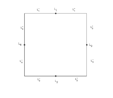
Figure 1: Geometrical setting: Boundaries and subsets of the boundaries of the square $S$.

At this moment, we can state the main result of this section; the existence of the chaotic saddle for the Lozi autonomous map.

Theorem 3.1.

For $a>4$ assumptions 1 and 2 hold for the autonomous Lozi map, and therefore it possesses a chaotic saddle inside the square $S$.

The proof of this theorem is carried out in the following subsections.

3.1 Verification of Assumption 1 of the Autonomous Conley-Moser Conditions

In this section we will show how the map $L$ acts on the square $S$. In order to do that, we want to see how the boundaries of the square $S$ are transformed. This action can be seen in figure 2.

First, we begin with the map $L$ acting on the upper boundary, $L_{1}$.

$$L(L_{1})=L(x,R)=(1+R-a|x|,-x)$$

$$\left\{\begin{array}[]{ccc}X&=&1+R-a|x|\\ Y&=&-x\\ \end{array}\right.$$

$$|y|=\frac{1+R-x}{a}\Rightarrow\left\{\begin{array}[]{cc}y=\frac{1+R}{a}-\frac{x}{a},&x<0\quad(L^{-}_{1})\\ &\\ y=\frac{x}{a}-\frac{1+R}{a},&x\geq 0\quad(L^{+}_{1})\\ \end{array}\right.$$ (23)

We do the same but for the lower boundary, $L_{2}$.

$$L(L_{2})=L(x,-R)=(1-R-a|x|,-x)$$

$$\left\{\begin{array}[]{ccc}X&=&1-R-a|x|\\ Y&=&-x\\ \end{array}\right.$$

$$|y|=\frac{1-R-x}{a}\Rightarrow\left\{\begin{array}[]{cc}y=\frac{1-R}{a}-\frac{x}{a},&x<0\quad(L^{-}_{2})\\ &\\ y=\frac{x}{a}-\frac{1-R}{a},&x\geq 0\quad(L^{+}_{2})\\ \end{array}\right.$$ (24)

Now we see the map $L$ acting on the right side, $L_{3}$.

$$L(L_{3})=L(R,y)=(1+y-aR,-R)$$

$$\left\{\begin{array}[]{ccc}X&=&1+y-aR\\ Y&=&-R\\ \end{array}\right.$$ (25)

and the left side, $L_{4}$.

$$L(L_{4})=L(-R,y)=(1+y-aR,R)$$

$$\left\{\begin{array}[]{ccc}X&=&1+y-aR\\ Y&=&R\\ \end{array}\right.$$ (26)

From these computations we can set that the horizontal boundaries $L_{1}$ and $L_{2}$ are mapped by $L$ to affine lines with slopes $|m|=1/a$ passing through the points $q=(1+R,0)$ and $p=(1-R,0)$ respectively that must be outside the domain $S$ as we will see later. Moreover, vertical lines are mapped to horizontal lines. From figure 2 we can observe how the strips are formed. In this case the set $L(S)\cap S$ is the union of the two horizontal strips $H_{1}$ and $H_{2}$.

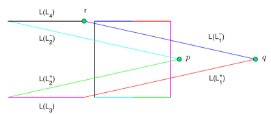
Figure 2: $L$ mapping $S$.

On the other hand, we want to show $L^{-1}$ acting on $S$, as is shown in figure 3. As we did before, we start with $L^{-1}$ acting on the upper side $L_{1}$.

$$L^{-1}(L_{1})=L^{-1}(x,R)=(-R,x+aR-1)$$

$$\left\{\begin{array}[]{ccc}X&=&-R\\ Y&=&x+aR-1\\ \end{array}\right.$$ (27)

and $L^{-1}$ acting on the lower side, $L_{2}$.

$$L^{-1}(L_{2})=L^{-1}(x,-R)=(R,x+aR-1)$$

$$\left\{\begin{array}[]{ccc}X&=&R\\ Y&=&x+aR-1\\ \end{array}\right.$$ (28)

Now we focus on $L^{-1}$ acting on the right side, $L_{3}$.

$$L^{-1}(L_{3})=L^{-1}(R,y)=(-y,R+a|y|-1)$$

$$\left\{\begin{array}[]{ccc}X&=&-y\\ Y&=&R+a|y|-1\\ \end{array}\right.$$

$$y=R+a|x|-1\Rightarrow\left\{\begin{array}[]{cc}y=R+ax-1,&y<0\quad(L^{-}_{3})\\ &\\ y=R-ax-1,&y\geq 0\quad(L^{+}_{3})\\ \end{array}\right.$$ (29)

and $L^{-1}$ acting on the left side, $L_{4}$.

$$L^{-1}(L_{4})=L^{-1}(-R,y)=(-y,-R+a|y|-1)$$

$$\left\{\begin{array}[]{ccc}X&=&-y\\ Y&=&-R+a|y|-1\\ \end{array}\right.$$

$$y=a|x|-(1+R)\Rightarrow\left\{\begin{array}[]{cc}y=ax-(1+R),&y<0\quad(L^{-}_{4})\\ &\\ y=-ax-(1+R),&y\geq 0\quad(L^{+}_{4})\\ \end{array}\right.$$ (30)

From this we can observe that the vertical boundaries $L_{3}$ and $L_{4}$ are mapped by $L^{-1}$ to affine lines with slopes $|m|=a$ passing through the points $\tilde{p}=(0,R-1)$ and $\tilde{q}=(0,-(1+R))$ respectively, which are outside the square, and horizontal lines are mapped to vertical lines. As we show in figure 3, the union of the vertical strips $V_{1}$ and $V_{2}$ is the set $L^{-1}(S)\cap S$.

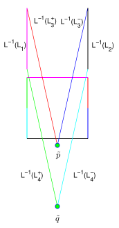
Figure 3: $L^{-1}$ mapping $S$.

Now that we know how the square $S$ is mapped under $L$ and $L^{-1}$ we have to set some conditions on the size of $S$, that is the value $R$. We have to keep in mind two conditions.

The first one is that we need the two horizontal strips and the two vertical strips to cross each other. (We illustrate this idea in figure 2). For that reason, we need the point $p$ to have first coordinate greater than $R$ and the point $\tilde{p}$ to have second coordinate lower than $-R$. Because of the symmetry of the problem, we reflect only the condition for $p$ in the next inequality

$$1-R\geq R\Leftrightarrow\frac{1}{2}\geq R$$ (31)

On the other hand, the second issue is that we need the area of intersection between the strips, represented for instance in figure 4, to be inside the domain $S$. This is achieved when the point $r=L(L_{1}^{-})\cap\{y=R\}$ has first coordinate lower than $-R$, as we can see in figure 2.

$$r=L(L_{1}^{-})\cap\{y=R\}=(1+R-a|x|,-x)|_{-x=R}=(1+R-aR,R)$$ (32)

So this last assumption is translated into

$$1+R-aR<-R$$ (33)

and this holds when

$$R\geq\frac{1}{a-2}$$ (34)

Combining these two conditions we have,

$$\frac{1}{a-2}\leq R\leq\frac{1}{2}$$ (35)

This last inequality only makes sense when $a\geq 4$.

Once we have set these conditions, we can take

$$R(a)=\frac{1}{2}\left(\frac{1}{a-2}+\frac{1}{2}\right)=\frac{a}{4(a-2)},\quad\text{for every }a\geq 4,$$ (36)

which is the midpoint of the interval

$$\left[\frac{1}{a-2},\quad\frac{1}{2}\right]$$

Now we start proving the first assumption, $A_{1}$, for the autonomous Conley-Moser conditions. For this purpose we need to define the vertical ($V_{1}$ and $V_{2}$) and the horizontal ($H_{1}$ and $H_{2}$) strips. To obtain the horizontal strips we will map forward by $L$ the square $S$ and make the intersection with the same square. To get the vertical strips we will map backward by $L^{-1}$ the square $S$ and intersect it with $S$, that is

$$\begin{array}[]{ccc}H_{1}\cup H_{2}&:=&L(S)\cap S\\ &&\\ V_{1}\cup V_{2}&:=&L^{-1}(S)\cap S\\ \end{array}$$ (37)

where $H_{1}$ is the upper half part of $L(S)\cap S$ and $H_{2}$ is the lower half part of $L(S)\cap S$, $V_{1}$ is the left half part of $L^{-1}(S)\cap S$ and $V_{2}$ is the right half part of $L^{-1}(S)\cap S$. We will use the following notation

$$\begin{array}[]{ccc}H_{1}&:=&(L(S)\cap S)^{+}\text{, where }y>0,\\ &&\\ H_{2}&:=&(L(S)\cap S)^{-}\text{, where }y<0,\\ &&\\ V_{1}&:=&(L^{-1}(S)\cap S)^{-}\text{, where }x<0,\\ &&\\ V_{2}&:=&(L^{-1}(S)\cap S)^{+}\text{, where }x>0,\\ \end{array}$$ (38)

These strips can be seen in figure 4.

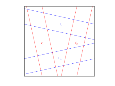
Figure 4: Vertical and horizontal strips. $H_{1}\cup H_{2}:=L(S)\cap S$ and $V_{1}\cup V_{2}:=L^{-1}(S)\cap S$.

It is easy to see from expressions in (38) that $L$ maps $V_{i}$ homeomorphically onto $H_{i}$, ($L(V_{i})=H_{i}$) for $i=1,2$. Furthermore, the horizontal boundaries of $V_{i}$ map to the horizontal boundaries of $H_{i}$ and the vertical boundaries of $V_{i}$ map to the vertical boundaries of $H_{i}$. Moreover, $V_{i}$ are $\mu_{v}$-vertical strips because its vertical boundaries are $\mu_{v}$-vertical curves where $|\mu_{v}|=1/a$. And $H_{i}$ are $\mu_{h}$-horizontal strips because its horizontal boundaries are $\mu_{h}$-horizontal curves where $|\mu_{h}|=1/a$.

Remark 3.2.

We have to take care about $|\mu_{v}|=1/a$. The slope of the vertical lines is $a$ but seen as horizontal curves. We must see this slope rate as if the vertical lines were $\mu_{v}$-vertical curves and so $|\mu_{v}|=1/a$.

We have to keep in mind that the product of the slopes of the strips has to be less than 1 as it is required in the Conley-Moser conditions. In our case $|\mu_{h}|=|\mu_{v}|=1/a$ Therefore

$$|\mu_{h}\cdot\mu_{v}|=|\frac{1}{a}\cdot\frac{1}{a}|=\frac{1}{a^{2}},$$ (39)

and the condition of the slopes of $A_{1}$ is satisfied.

3.2 Verification of Assumption 2 of the Autonomous Conley-Moser Conditions.

The second assumption describes how the map $L$ bends and makes thinner strips on each iteration. Moreover we obtain this rate which in our assumption is called $\nu_{v}$. Lets take $V$ a $\mu_{v}$-vertical strip contained, for instance, in $V_{2}$ ($V\subset V_{2}$). As we can see in figure 5, we name the vertices of $V_{2}$ as $v_{1}=(v_{1_{x}},R)$, $v_{2}=(v_{2_{x}},R)$, $v_{3}=(v_{3_{x}},-R)$ and $v_{4}=(v_{4_{x}},-R)$ and the vertices which delimit $V$ are $q_{1}=(q_{1_{x}},R)$, $q_{2}=(q_{2_{x}},R)$, $q_{3}=(q_{3_{x}},-R)$ and $q_{4}=(q_{4_{x}},-R)$. We assume that

$$\begin{array}[]{ccccccc}v_{1_{x}}&<&q_{1_{x}}&<&q_{2_{x}}&<&v_{2_{x}}\\ v_{3_{x}}&<&q_{3_{x}}&<&q_{4_{x}}&<&v_{4_{x}}\\ \end{array}$$ (40)

and

$$d(V)=|q_{2_{x}}-q_{1_{x}}|=|q_{4_{x}}-q_{3_{x}}|$$

The vertical boundaries of $V$ are the straight lines with slope rate $a$ (because $V$ is $\mu_{v}$-vertical strip) and pass through the points $q_{1}$ and $q_{2}$ respectively:

$$\begin{array}[]{l}y_{q_{1}}=ax+R-aq_{1_{x}}\\ y_{q_{2}}=ax+R-aq_{2_{x}}\\ \end{array}$$ (41)

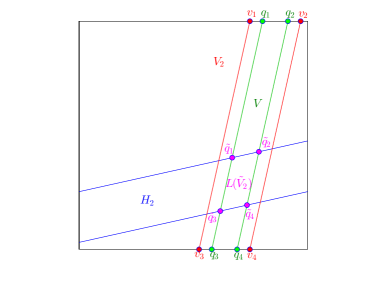
Figure 5: $V\subset V_{2}$ strip and $L(\tilde{V}_{2})\equiv V\cap H_{2}$.

We need to determine $\tilde{V}_{2}\equiv L^{-1}(V)\cap V_{2}$. Since we do not know how $L^{-1}$ acts on $V$, first we obtain $L(\tilde{V}_{2})\equiv V\cap L(V_{2})=V\cap H_{2}$ and after that, we will recover $\tilde{V}_{2}$ by iterating $L(\tilde{V}_{2})$ backward. $V$ cuts $H_{2}$ at four points: $\tilde{q}_{1}$, $\tilde{q}_{2}$, $\tilde{q}_{3}$ and $\tilde{q}_{4}$ and we can describe them as follows:

$$\tilde{q}_{1}:y_{q_{1}}\cap\left\{y=\frac{x-(1-R)}{a}\right\}\Rightarrow\left\{\begin{array}[]{l}y=\frac{x-(1-R)}{a}\\ \\ y=ax+R-aq_{1_{x}}\\ \end{array}\right.$$ (42)

Solving these two equations gives the coordinates of $\tilde{q}_{1}$:

$$\begin{array}[]{l}\tilde{q}_{1_{x}}=\frac{a^{2}q_{1_{x}}-aR-1+R}{a^{2}-1}\\ \\ \tilde{q}_{1_{y}}=\frac{aq_{1_{x}}+aR-a-R}{a^{2}-1}\end{array}$$ (43)

We continue the same procedure for the rest of the points

$$\tilde{q}_{2}:y_{q_{2}}\cap\left\{y=\frac{x-(1-R)}{a}\right\}\Rightarrow\left\{\begin{array}[]{l}y=\frac{x-(1-R)}{a}\\ \\ y=ax+R-aq_{2_{x}}\\ \end{array}\right.$$ (44)

and the coordinates for $\tilde{q}_{2}$ are

$$\begin{array}[]{l}\tilde{q}_{2_{x}}=\frac{a^{2}q_{2_{x}}-aR-1+R}{a^{2}-1}\\ \\ \tilde{q}_{2_{y}}=\frac{aq_{2_{x}}+aR-a-R}{a^{2}-1}\end{array}$$ (45)

In the case of $\tilde{q}_{3}$ we solve

$$\tilde{q}_{3}:y_{q_{1}}\cap\left\{y=\frac{x-(1+R)}{a}\right\}\Rightarrow\left\{\begin{array}[]{l}y=\frac{x-(1+R)}{a}\\ \\ y=ax+R-aq_{1_{x}}\\ \end{array}\right.$$ (46)

with coordinates

$$\begin{array}[]{l}\tilde{q}_{3_{x}}=\frac{a^{2}q_{1_{x}}-aR-1-R}{a^{2}-1}\\ \\ \tilde{q}_{3_{y}}=\frac{aq_{1_{x}}-aR-a-R}{a^{2}-1}\end{array}$$ (47)

Finally, to obtain $\tilde{q}_{4}$ we solve the system

$$\tilde{q}_{4}:y_{q_{2}}\cap\left\{y=\frac{x-(1+R)}{a}\right\}\Rightarrow\left\{\begin{array}[]{l}y=\frac{x-(1+R)}{a}\\ \\ y=ax+R-aq_{2_{x}}\\ \end{array}\right.$$ (48)

therefore its coordinates are

$$\begin{array}[]{l}\tilde{q}_{4_{x}}=\frac{a^{2}q_{2_{x}}-aR-1-R}{a^{2}-1}\\ \\ \tilde{q}_{4_{y}}=\frac{aq_{2_{x}}-aR-a-R}{a^{2}-1}\end{array}$$ (49)

At this moment, we have given a precise description of $L(\tilde{V}_{2})$; it is a strip delimited by the four vertices from above and the straight lines $y_{q_{1}}$, $y_{q_{2}}$, $y=\frac{x-(1-R)}{a}$ and $y=\frac{x-(1+R)}{a}$. In order to recover $\tilde{V}_{2}$ we should map it backward by $L^{-1}$. By continuity, and since $L$ is orientation preserving, the points which are leading to $y=R$ are $L^{-1}(\tilde{q}_{4})$ and $L^{-1}(\tilde{q}_{3})$ and the points that are mapped to $y=-R$ are $L^{-1}(\tilde{q}_{2})$ and $L^{-1}(\tilde{q}_{1})$, and therefore

$$d(\tilde{V}_{2})=|L^{-1}(\tilde{q}_{4_{x}})-L^{-1}(\tilde{q}_{3_{x}})|=|L^{-1}(\tilde{q}_{2_{x}})-L^{-1}(\tilde{q}_{1_{x}})|$$ (50)

For instance we compute $L^{-1}(\tilde{q}_{4_{x}})$ and $L^{-1}(\tilde{q}_{3_{x}})$

$$\begin{array}[]{ccl}L^{-1}(\tilde{q}_{4_{x}})&=&L^{-1}(\frac{a^{2}\tilde{q}_{2_{x}}-aR-1-R}{a^{2}-1},\frac{a\tilde{q}_{2_{x}}-aR-a-R}{a^{2}-1})\\ &&\\ &=&(\frac{aR+a+R-a\tilde{q}_{2_{x}}}{a^{2}-1},\frac{a^{2}\tilde{q}_{2_{x}}-aR-1-R}{a^{2}-1}+\frac{a|a\tilde{q}_{2_{x}}-aR-a-R|}{a^{2}-1}-1)\\ &&\\ &\stackrel{{\scriptstyle(*)}}{{=}}&(\frac{aR+a+R-a\tilde{q}_{2_{x}}}{a^{2}-1},\frac{a^{2}q_{2_{x}}-aR-1-R-a^{2}q_{2_{x}}+a^{2}R+a^{2}+aR-a^{2}+1}{a^{2}-1})\\ &&\\ &=&(\frac{aR+a+R-a\tilde{q}_{2_{x}}}{a^{2}-1},R)\\ \end{array}$$ (51)

In $(*)$ we have use the fact that $a\tilde{q}_{2_{x}}-aR-a-R<0$ as $\tilde{q}_{2_{x}}<R$ and $a>0$. The computations for $L^{-1}(\tilde{q}_{2})$ are analogous, so

$$L^{-1}(\tilde{q}_{3_{x}})=(\frac{a+aR+R-aq_{1_{x}}}{a^{2}-1},R)$$ (52)

Using (50), we can compute $d(\tilde{V}_{2})$

$$\begin{array}[]{ccl}d(\tilde{V}_{2})&=&\displaystyle{\frac{|a+aR+R-aq_{1_{x}}-a-aR-R+aq_{2_{x}}|}{a^{2}-1}}\\ &&\\ &=&\displaystyle{\frac{a}{a^{2}-1}\cdot|q_{2_{x}}-q_{1_{x}}|=\nu_{v}\cdot d(V)}\end{array}$$ (53)

Therefore we only need the rate $\nu_{v}$ to be less than 1 and that holds when $a>\frac{1+\sqrt{5}}{2}$:

$$\frac{a}{a^{2}-1}<1\Leftrightarrow a^{2}-a-1>0\Leftrightarrow a>\frac{1+\sqrt{5}}{2}=\Phi$$ (54)

The last issue of assumption 2 that remains to be proved is that $\tilde{V}_{i}$ is a $\mu_{v}$-vertical strip. In order to prove this we realize that $L(\tilde{V}_{i})=V\cap L(V_{i})=V\cap H_{i}$ is a $\mu_{h}$-horizontal strip since its boundaries are $\mu_{h}$-horizontal curves. As we know by assumption 1, by $F^{-1}$ horizontal boundaries of horizontal strips map to horizontal boundaries of vertical strips and vertical boundaries of vertical strips map to vertical boundaries of horizontal strips and it is clear that this vertical boundaries of $\tilde{V}_{i}$ are $\mu_{v}$-horizontal curves. Therefore the second assumption is already proven and hence, using Theorem 3.1, the existence of the chaotic saddle inside $S$ is proven.

4 Non-autonomous Lozi map

In this section we prove that Assumptions 1 and 3 of the nonautonomous Conley-Moser conditions hold for the nonautonomous Lozi map. We begin by developing the set-up for the problem. We define the maps $L_{n}$ and the domains $S_{n}$ as follows:

$$L_{n}(x,y)=(1+y-a(n)|x|,\quad-x)$$ (55)

and

$$L^{-1}_{n}(x,y)=(-y,\quad x+a(n)|y|-1)$$ (56)

where $a(n)=a+\epsilon(1+\cos(n))$, $a>4$. The domains can be set as $S_{n}=[-R(n),R(n)]\times[-R(n),R(n)]$ where

$$R(n)=\frac{a(n)}{4(a(n)-2)}$$ (57)

Although the domain may change with each iteration, in this example we can consider a fixed domain in order to simplify the proof of Theorem 4.1. Therefore we define the domain as:

$$S=\sup_{n\in\mathbb{Z}}([-R(n),R(n)]\times[-R(n),R(n)])=[-R,R]\times[-R,R]$$ (58)

where

$$R=\sup_{n\in\mathbb{Z}}\frac{a(n)}{4(a(n)-2)}.$$ (59)

To find this value we examine the monotonicity of the function

$$f(a(n))=\frac{a(n)}{4(a(n)-2)}$$ (60)

for $a(n)\neq 2$. This function always decreases since its derivate is negative when $a(n)\neq 2$. Therefore the supreme of this value is determined from the following relations:

$$\inf_{n\in\mathbb{Z}}a(n)=a+\epsilon(1-1)=a.$$ (61)

and

$$R=\sup_{n\in\mathbb{Z}}R(n)=\frac{\inf_{n\in\mathbb{Z}}a(n)}{4(\inf_{n\in\mathbb{Z}}a(n)-2)}=\frac{a}{4(a-2)}$$ (62)

As we did in the autonomous case, we must check conditions similar to inequalities (31) and (33) in order to obtain strips of four vertices totally included in the maximal domain $S$.

By the symmetry of the problem, as it is shown in figure 4, the first condition, (31), is satisfied since the point $p$ does not depend on the iteration $n$. So this condition holds when

$$R<\frac{1}{2}.$$ (63)

The second condition is analogous to (33), and is also holds. We want the point $r$ to cut the horizontal line $y=R$ out from the domain $S$ and it must have first coordinate lower than $-R$.

$$r=L_{n}(L_{1}^{-})\cap\{y=R\}=(1+R-a(n)|x|,-x)|_{-x=R}=(1+R-a(n)R,R)$$ (64)

therefore we must determine if the following inequality holds

$$1+R-a(n)R<-R\Leftrightarrow 1<(a(n)-2)R\quad\text{for all }n\in\mathbb{Z}$$ (65)

and it does hold since

$$(a(n)-2)R>(a-2)\frac{a}{4(a-2)}=\frac{a}{4}>1$$ (66)

when $a>4$ for all $n\in\mathbb{Z}$.

Henceforth, we set $S=S_{n}$ for all $n\in\mathbb{Z}$ and we can state the main nonautonomous theorem.

Theorem 4.1.

For $a(n)=a+\epsilon(1+\cos(n))$ where $a>4$ and $\epsilon$ small, Assumptions 1 and 3 of the nonautonomous Conley-Moser conditions hold for the nonautonomous Lozi map $L_{n}$. and therefore it possesses a chaotic saddle, $\Lambda_{n}$, inside the square $S$. In other words, $\left\{\Lambda_{n},L_{n}\right\}^{+\infty}_{n=-\infty}$ is a infinite sequence of chaotic invariant sets where

$$\Lambda\equiv\cup_{n\in\mathbb{Z}}\Lambda_{n},$$

contains an uncountable infinity or orbits, each of them unstable (of saddle type) and the dynamics on the invariant set exhibits sensitive dependence on initial conditions.

From now to on, we see how these two assumptions are held. First of all, we construct the horizontal and vertical strips as in the autonomous case. Then, we check the third assumption, the cone condition, to quantify the folding and stretching of the strips.

4.1 Verification of Assumption 1 for the nonautonomous Conley-Moser Conditions

We have defined the bi-infinite sequence of maps and domains

$$\left\{L_{n},S\right\}^{+\infty}_{n=-\infty},\qquad L_{n}:S\rightarrow\mathbb{R}^{2}$$ (67)

satisfying

$$L_{n}(S)\cap S\neq\emptyset,\quad\forall n\in\mathbb{Z}.$$

Now we define the main geometrical structures of this problem, the horizontal and the vertical strips. In this context we will proceed as in the autonomous case adding the iteration variable

$$\begin{array}[]{ccc}H^{n+1}_{1}\cup H^{n+1}_{2}&:=&L_{n}(S)\cap S\\ &&\\ V^{n}_{1}\cup V^{n}_{2}&:=&L^{-1}_{n}(S)\cap S\\ \end{array}$$ (68)

where $H^{n+1}_{1}$ is the upper half part of $L_{n}(S)\cap S$ and $H^{n+1}_{2}$ is the lower half part of $L_{n}(S)\cap S$, $V^{n}_{1}$ is the left half part of $L^{-1}_{n}(S)\cap S$ and $V^{n}_{2}$ is the right half part of $L^{-1}_{n}(S)\cap S$. We will use the following notation

$$\begin{array}[]{ccc}H^{n+1}_{1}&:=&(L_{n}(S)\cap S)^{+}\text{, where }y>0,\\ &&\\ H^{n+1}_{2}&:=&(L_{n}(S)\cap S)^{-}\text{, where }y<0,\\ &&\\ V^{n}_{1}&:=&(L^{-1}_{n}(S)\cap S)^{-}\text{, where }x<0,\\ &&\\ V^{n}_{2}&:=&(L^{-1}_{n}(S)\cap S)^{+}\text{, where }x>0.\\ \end{array}$$ (69)

We are giving only the vertices of $H^{n+1}_{1}$ and $V^{n}_{1}$. The vertices of $H^{n+1}_{2}$ and $V^{n}_{2}$ are symmetric with respect to $y=0$ and $x=0$ respectively. We show $H^{n+1}_{i}$ and $V^{n}_{i}$ in figure 6.

$$h_{11}:\{x=-R\}\cap\left\{y=\frac{1+R-x}{a(n)}\right\}\Rightarrow\left\{\begin{array}[]{l}h_{11_{x}}=-R\\ \\ h_{11_{y}}=\frac{1+2R}{a(n)}\\ \end{array}\right.$$ (70)

$$h_{12}:\{x=R\}\cap\left\{y=\frac{1+R-x}{a(n)}\right\}\Rightarrow\left\{\begin{array}[]{l}h_{12_{x}}=R\\ \\ h_{12_{y}}=\frac{1}{a(n)}\\ \end{array}\right.$$ (71)

$$h_{13}:\{x=R\}\cap\left\{y=\frac{1-R-x}{a(n)}\right\}\Rightarrow\left\{\begin{array}[]{l}h_{13_{x}}=R\\ \\ h_{13_{y}}=\frac{1-2R}{a(n)}\\ \end{array}\right.$$ (72)

$$h_{14}:\{x=-R\}\cap\left\{y=\frac{1-R-x}{a(n)}\right\}\Rightarrow\left\{\begin{array}[]{l}h_{14_{x}}=-R\\ \\ h_{14_{y}}=\frac{1}{a(n)}\\ \end{array}\right.$$ (73)

and the computations for the vertices of $V^{n}_{1}$ are similar

$$v_{11}:\{y=R\}\cap\left\{y=-R-a(n)x-1\right\}\Rightarrow\left\{\begin{array}[]{l}v_{11_{x}}=\frac{-2R-1}{a(n)}\\ \\ v_{11_{y}}=R\\ \end{array}\right.$$ (74)

$$v_{12}:\{y=R\}\cap\left\{y=R-a(n)x-1\right\}\Rightarrow\left\{\begin{array}[]{l}v_{12_{x}}=\frac{-1}{a(n)}\\ \\ v_{12_{y}}=R\\ \end{array}\right.$$ (75)

$$v_{13}:\{y=-R\}\cap\left\{y=R-a(n)x-1\right\}\Rightarrow\left\{\begin{array}[]{l}v_{13_{x}}=\frac{2R-1}{a(n)}\\ \\ v_{13_{y}}=-R\\ \end{array}\right.$$ (76)

$$v_{14}:\{y=-R\}\cap\left\{y=-R-a(n)x-1\right\}\Rightarrow\left\{\begin{array}[]{l}v_{14_{x}}=\frac{-1}{a(n)}\\ \\ v_{14_{y}}=-R\\ \end{array}\right.$$ (77)

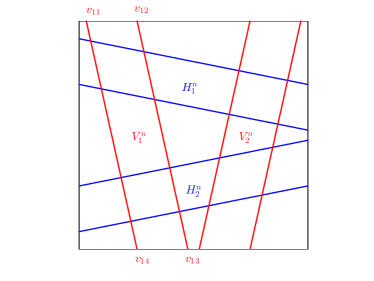
(a) $\quad n_{0}=n$

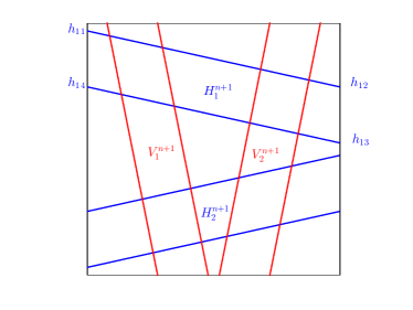
(b) $\quad n_{0}=n+1$

Figure 6: Vertical and horizontal strips. $L_{n}(V^{n}_{i})=H^{n+1}_{i},\quad i=1,2$.

As it is defined above, $V^{n}_{i}$ and $H^{n+1}_{i}$ are $\mu^{n}_{v}$-vertical strips and $\mu^{n+1}_{h}$-horizontal strips respectively with $\mu^{n}_{v}=1/a(n)$ and $\mu^{n+1}_{h}=1/a(n+1)$. Taking into account Remark 4.2 and due to reasons explained afterwards, by convenience, we can choose

$$\mu_{v}=\mu_{h}=\frac{a-\sqrt{a^{2}-4}}{2}>1/a(n),$$ (78)

for all $n\in\mathbb{Z}$ and $a>4$.

Remark 4.2.

Note that if $V$ is a $\mu_{v}$-vertical strip and $\mu_{v}\leq\mu^{*}_{v}$, therefore $V$ is a $\mu^{*}_{v}$-vertical strip:

$$|x_{1}-x_{2}|\leq\mu_{v}|y_{1}-y_{2}|\leq\mu^{*}_{v}|y_{1}-y_{2}|.$$

The same argument could be done for horizontal strips.

$L_{n}$ is a homeomorphism on the whole plane and so on $S$. Therefore

$$L_{n}(V^{n}_{i})=H^{n+1}_{i},\quad i=1,2.$$ (79)

We should also define

$$\begin{array}[]{rcl}L_{n}(V^{n}_{i})\cap V^{n+1}_{j}&\equiv&H^{n+1}_{ij}\\ &&\\ V^{n}_{i}\cap L^{-1}_{n}(V^{n+1}_{j})&\equiv&L^{-1}_{n}(H^{n+1}_{ij})\equiv V^{n}_{ji}\\ \end{array}$$ (80)

Let $\left\{A^{n}\right\}^{+\infty}_{n=-\infty}$ denote a sequence of $2\times 2$ matrices such that

$$A^{n}_{ij}=\left\{\begin{array}[]{ccc}0&\text{if}&L_{n}(V^{n}_{i})\cap V^{n+1}_{j}=H^{n+1}_{i}\cap V^{n+1}_{j}=\emptyset\\ &&\\ 1&\text{if}&L_{n}(V^{n}_{i})\cap V^{n+1}_{j}=H^{n+1}_{i}\cap V^{n+1}_{j}\neq\emptyset\\ \end{array}\right.$$ (81)

In our case, we can ensure that

$$A^{n}=\left(\begin{array}[]{cc}1&1\\ 1&1\\ \end{array}\right)$$ (82)

We know that $H^{n+1}_{i}$ are horizontal strips formed by two $\mu_{h}$-horizontal curves that rest on the lines $x=R$ and $x=-R$ and $V^{n+1}_{j}$ are vertical strips formed by two $\mu_{v}$-vertical curves that lead from $y=R$ to $y=-R$. So applying the Fixed Point Theorem, these straight lines get cut in four vertices that together with the two horizontal and the two vertical lines form $H^{n+1}_{ij}$. These sets are $\mu_{h}$-horizontal strips because its boundaries are contained in $V^{n+1}_{j}$ due to its construction ($H^{n+1}_{i}\cap V^{n+1}_{j}$).

Furthermore, due to the fact that $L_{n}$ is homeomorphism and the construction of the strips, $L_{n}$ maps $V^{n}_{ji}$ onto $H^{n+1}_{ij}$. It is clear from (80) that

$$L^{-1}_{n}(H^{n+1}_{ij})=V^{n}_{ji}=L^{-1}_{n}(V^{n+1}_{j})\cap V^{n}_{i}\Longrightarrow L^{-1}_{n}(H^{n+1}_{ij})\subset V^{n}_{i}$$ (83)

so

$$L_{n}^{-1}(\partial_{h}H_{ij}^{n+1})\subset\partial_{h}V_{i}^{n}.$$ (84)

Finally we need to prove $\mu_{v}\mu_{h}<1$. We know that $\mu_{v}=\mu_{h}=\frac{a-\sqrt{a^{2}-4}}{2}$ and

$$\mu_{v}\cdot\mu_{h}=\displaystyle{\left(\frac{a-\sqrt{a^{2}-4}}{2}\right)^{2}}<1$$ (85)

so Assumption 1 is proven.

4.2 The Cone Condition. Assumption A3 of the Nonautonomous Conley-Moser Conditions

As we stated earlier, the second assumption of the Conley-Moser conditions can be replaced by another condition named the cone condition. Given any point $z_{0}=(x_{0},y_{0})\in{\cal H}^{n+1}$ and any $(\xi_{z_{0}},\eta_{z_{0}})\in S^{s}_{{\cal H}^{n+1}}$ (which by definition, $|\xi_{z_{0}}|\leq\mu_{v}|\eta_{z_{0}}|$) we have that

$$DL^{-1}_{n}(z_{0})\cdot(\xi_{z_{0}},\eta_{z_{0}})=\left(\begin{array}[]{cc}0&-1\\ 1&a(n)sign(y)\\ \end{array}\right)\left(\begin{array}[]{c}\xi_{z_{0}}\\ \eta_{z_{0}}\\ \end{array}\right)=\left(\begin{array}[]{c}-\eta_{z_{0}}\\ \xi_{z_{0}}+a(n)sign(y)\eta_{z_{0}}\\ \end{array}\right)$$ (86)

and (86) belongs to $S^{s}_{{\cal V}^{n}}$ if and only if the inequality

$$|-\eta_{z_{0}}|=|\eta_{z_{0}}|\leq\mu_{v}|\xi_{z_{0}}+a(n)sign(y)\eta_{z_{0}}|$$ (87)

holds and this is true since

$$\begin{array}[]{rcl}\mu_{v}|\xi_{z_{0}}+a(n)sign(y)\eta_{z_{0}}|\geq\mu_{v}(a(n)|\eta_{z_{0}}|-|\xi_{z_{0}}|)&\geq&\\ &&\\ \mu_{v}(a(n)|\eta_{z_{0}}|-\mu_{v}|\eta_{z_{0}}|)=\mu_{v}(a(n)-\mu_{v})|\eta_{z_{0}}|&\stackrel{{\scriptstyle(*)}}{{\geq}}&|\eta_{z_{0}}|\\ \end{array}$$ (88)

Last part of the inequality, (*), holds when $\mu_{v}(a(n)-\mu_{v})\geq 1$ and that is satisfied when

$$\mu_{v}\in\left[\frac{a(n)-\sqrt{a(n)^{2}-4}}{2},\quad\frac{a(n)+\sqrt{a(n)^{2}-4}}{2}\right]=I_{n}$$ (89)

We need to prove that $\mu_{v}\in I_{n}$ for every $n\in\mathbb{Z}$, or, equivalently

$$\begin{array}[]{rcl}\mu_{v}\in\bigcap_{n\in\mathbb{Z}}I_{n}&=&\left[\sup_{n\in\mathbb{Z}}\frac{a(n)-\sqrt{a(n)^{2}-4}}{2},\quad\inf_{n\in\mathbb{Z}}\frac{a(n)+\sqrt{a(n)^{2}-4}}{2}\right]\\ &&\\ &=&\left[\displaystyle{\frac{a-\sqrt{a^{2}-4}}{2}},\quad\displaystyle{\frac{a+\sqrt{a^{2}-4}}{2}}\right]\\ \end{array}$$ (90)

Finally we can set a general value for $\mu_{h}$ and $\mu_{v}$ that hold for the last inequalities

$$\mu_{h}=\mu_{v}=\frac{a-\sqrt{a^{2}-4}}{2}$$ (91)

and we can observe that

$$\mu_{h}\cdot\mu_{v}=\displaystyle{\left(\frac{a-\sqrt{a^{2}-4}}{2}\right)^{2}}<1$$ (92)

Since $z_{0}\in{\cal H}^{n+1}$ is an arbitrary point, the inclusion $DL^{-1}_{n}(S^{s}_{{\cal H}^{n+1}})\subset S^{s}_{{\cal V}^{n}}$ is proven.

To finish the proof of Assumption 3, we only need to prove the inequality

$$|\eta_{{f}^{-1}_{n}(z_{0})}|\geq\frac{1}{\mu}|\eta_{z_{0}}|$$ (93)

for $0<\mu<1-\mu_{h}\mu_{v}$ and $z_{0}\in{\cal H}^{n+1}$, $(\xi_{z_{0}},\eta_{z_{0}})\in S^{s}_{{\cal H}^{n+1}}$ because

$$|\xi_{{f}_{n}(z_{0})}|\geq\frac{1}{\mu}|\xi_{z_{0}}|,\quad z_{0}\in{\cal V}^{n},\quad(\xi_{z_{0}},\eta_{z_{0}})\in S^{u}_{{\cal V}^{n}}$$ (94)

is proved by using a similar argument.

$$\begin{array}[]{rcl}|\eta_{{f}^{-1}_{n}(z_{0})}|\geq|\xi_{z_{0}}+a(n)sign(y)\eta_{z_{0}}|\geq a(n)|\eta_{z_{0}}|-|\xi_{z_{0}}|&\geq&\\ &&\\ a(n)|\eta_{z_{0}}|-\mu_{v}|\eta_{z_{0}}|=(a(n)-\mu_{v})|\eta_{z_{0}}|&\geq&\frac{1}{\mu}|\eta_{z_{0}}|\\ \end{array}$$ (95)

so it follows that

$$\mu\geq\frac{1}{a(n)-\mu_{v}}.$$ (96)

Taking into account this last inequality and the condition $0<\mu<1-\mu_{h}\mu_{v}$, we have the following chain of inequalities

$$\frac{1}{a(n)-\mu_{v}}\leq\mu\leq 1-\mu_{h}\mu_{v}$$ (97)

and this last inequality is satisfied providing that $a>4$ so the proof of the Assumption 3 is complete.

The proof of the second inclusion $DL_{n}(S^{u}_{{\cal V}^{n}})\subset S^{u}_{{\cal H}^{n+1}}$ is similar.

5 The visualization of the Chaotic Saddle.

In this section the chaotic saddle for the autonomous and for the non-autonomous cases are displayed by using the discrete Lagrange descriptors (DLD). This tool explained in Lopesino, et al. [2015] consists of evaluating the $p$-norm of an orbit generated by a two dimensional map, in our case the Lozi map. For instance, let

$$\left\{x_{n},y_{n}\right\}^{n=N}_{n=-N},\quad N\in\mathbb{N},$$ (98)

denote an orbit of a point. The DLD is defined as follows:

$$MD_{p}=\displaystyle{\sum^{N-1}_{i=-N}|x_{i+1}-x_{i}|^{p}+|y_{i+1}-y_{i}|^{p}},\quad p\leq 1.$$ (99)

We are interested on showing the phase space where the chaotic saddle exists, therefore our study region is the square $S$. We prepare a set of initial conditions by fixing a spatial grid and then expression (99) is applied to the initial conditions belonging to this grid.

The Chaotic Saddle for the autonomous case. Figure 7 shows the chaotic saddle of the Lozi map for different values of $a$. It is confirmed that only when $a\geq 4$, the set is wholly contained in the square S.

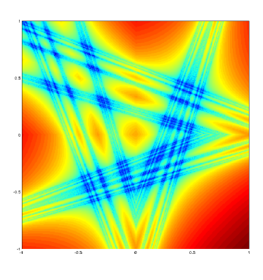
(a)     Chaotic S with a=3

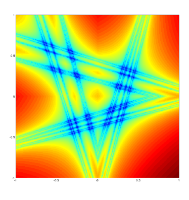
(b)     Chaotic S with a=3.5

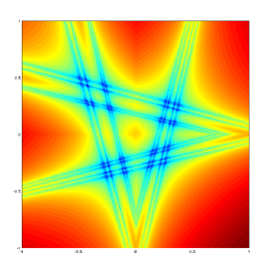
(c)     Chaotic S with a=4

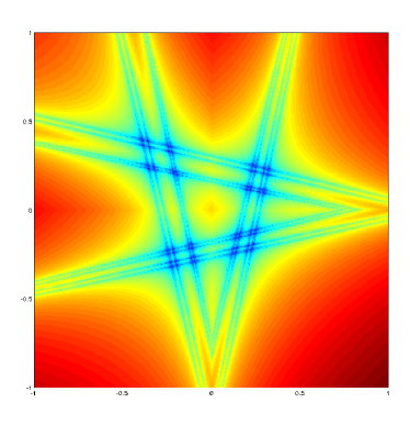
(d)     Chaotic S with a=4.5

Figure 7: Chaotic saddle for different values of $a$. These panels show contours of $MD_{p}$ for $p=0.25$ and $N=20$, with a grid point spacing of $0.005$.

The Chaotic Saddle for the non autonomous case. Figure 8 shows by means of the DLD tool, how the chaotic saddle evolves with the iterations when the autonomous system is perturbed.

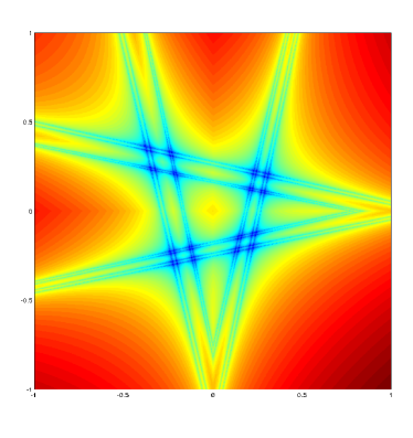
(a)     Chaotic S. with $n_{0}=-3$

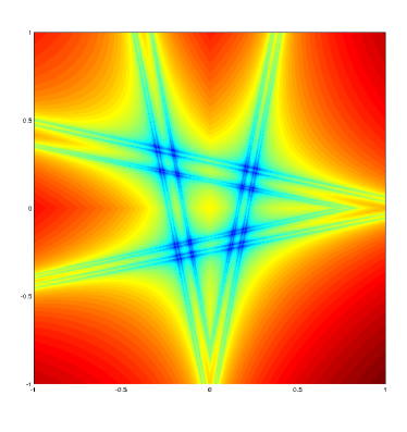
(b)     Chaotic S. with $n_{0}=-1$

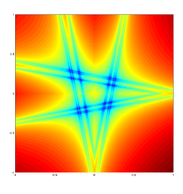
(c)     Chaotic S. with $n_{0}=1$

(d)     Chaotic S. with $n_{0}=3$

Figure 8: Chaotic saddle for different starting time iteration. These panels show contours of $MD_{p}$ for $p=0.25$, $A=4.5+\epsilon(1+\cos(n))$ and $N=100$, with a grid point spacing of $0.001$.

6 Summary and Conclusions

In this paper we have considered the Lozi map, both in its autonomous and nonautonomous versions, and provided necessary conditions for the map to possess a chaotic invariant set. This is accomplished by using autonomous and nonautonomous versions of the Conley-Moser conditions, in particular we used the sharpened conditions for nonautonomous maps given in Balibrea-Iniesta, et al. [2015] to show that the nonautonomous chaotic invariant set is hyperbolic. In the course of the proof we provide a precise characterization of what is meant by the phrase ”hyperbolic chaotic invariant set” for nonautonmous dynamical systems. At the end of this paper we have used the DLD to visualize the chaotic saddle for different parameters.

References

- Alekseev [1968a] Alekseev, V.M. (1968a). Quasirandom dynamical systems, I. Math. USSR-Sb , 5, 73-128.
- Alekseev [1968b] Alekseev, V.M. (1968b). Quasirandom dynamical systems, II. Math. USSR-Sb , 6, 505-560.
- Alekseev [1969] Alekseev, V.M. (1969). Quasirandom dynamical systems, III. Math. USSR-Sb , 6, 1-43.
- Balibrea-Iniesta, et al. [2015] Balibrea-Iniesta, F., Lopesino, C., Wiggins S., Mancho A.M. (2015). Chaotic dynamics in nonautonomous maps: Application to the nonautonomous Hénon map. International Journal of Bifurcation and Chaos (in press).
- Chastaing, et al. [2014] Chastaing J. -Y., Bertin E. and Géminard J. -C. (2014). Dynamics of the bouncing ball. http://arxiv.org/pdf/1405.3482v1.pdf
- Devaney and Nitecki [1979] Devaney, R. and Nitecki, Z. (1979). Shift automorphisms in the hénon mapping. Comm. Math. Phys., 67, 137–179.
- Holmes [1982] Holmes P. J. (1982). The dynamics of repeated impacts with a sinusoidally vibrating table. Journal of Sound and Vibration, 84(2), 173-189.
- Lerman and Silnikov [1992] Lerman, L. and Silnikov, L. (1992). Homoclinical structures in nonautonomous systems: Nonautonomous chaos. Chaos, 2, 447–454.
- Lopesino, et al. [2015] Lopesino C., Balibrea F., Wiggins S., Mancho A. (2015). Lagrangian Descriptors for Two Dimensional, Area Preserving, Autonomous and Nonautonomous Maps. Communications in Nonlinear Science and Numerical Simulation 27 (1-3) 40–51.
- Lozi [1978] Lozi, R. (1978). Un attracteur etrange (?) du type attracteur de Henon. Journal de Physique Colloques, 39, pp.C5-9-C5-10.
- Moser [1973] Moser, J. (1973). Stable and Random Motions in Dynamical Systems. Annals of mathematical studies, 77. Princeton University Press.
- Stoffer [1988a] Stoffer, D. (1988a). Transversal homoclinic points and hyperbolic sets for non-autonomous maps I. J. Appl. Math. and Phys. (ZAMP), 39, 518–549.
- Stoffer [1988b] Stoffer, D. (1988b). Transversal homoclinic points and hyperbolic sets for non-autonomous maps II. J. Appl. Math. and Phys. (ZAMP), 39, 783–812.
- Wiggins [1999] Wiggins S. (1999). Chaos in the dynamics generated by sequences of maps, with applications to chaotic advection in flows with aperiodic time dependence. Z. angew. Math. Phys. (ZAMP), 50, 585–616.
- Wiggins [2003] Wiggins S. (2003). Introduction to Applied Nonlinear Dynamical Systems and Chaos. Springer Second Edition.
- Wiggins and Mancho [2014] Wiggins, S and Mancho, A. M. (2014). Barriers to transport in aperiodically time-dependent two-dimensional velocity fields: Nekhoroshev’s theorem and ‘’nearly invariant” tori. Nonlinear Processes in Geophysics, 21, 165–185.