Pulsar Timing and its application for Navigation and Gravitational Wave Detection

Abstract

Pulsars are natural cosmic clocks. On long timescales they rival the precision of terrestrial atomic clocks. Using a technique called pulsar timing, the exact measurement of pulse arrival times allows a number of applications, ranging from testing theories of gravity to detecting gravitational waves. Also an external reference system suitable for autonomous space navigation can be defined by pulsars, using them as natural navigation beacons, not unlike the use of GPS satellites for navigation on Earth. By comparing pulse arrival times measured on-board a spacecraft with predicted pulse arrivals at a reference location (e.g. the solar system barycenter), the spacecraft position can be determined autonomously and with high accuracy everywhere in the solar system and beyond. We describe the unique properties of pulsars that suggest that such a navigation system will certainly have its application in future astronautics. We also describe the on-going experiments to use the clock-like nature of pulsars to “construct” a galactic-sized gravitational wave detector for low-frequency ($f_{GW}\sim 10^{-9}-10^{-7}$ Hz) gravitational waves. We present the current status and provide an outlook for the future.

1 Introduction

For millenia, keeping time was safely in the hands of astronomers, who watched the heavens to serve the societies’ needs for time measurements. They used the Earth’s rotation, the moon, the Sun and the stars to keep time, but, of course, they also exploited their observations to study and explore the Universe that we live in. Practical purposes, especially the need to navigate, turned the art of timekeeping into the hands of clockmakers and, hence, engineers and physicists. Today, world time is kept by a set of ultra-precise atomic clocks, and the sophistication and accuracy of these clocks is hugely impressive (see other contributions to this book). The stability of these clocks is best on small timescales. When time stability is needed on long timescales, one can (and does) “hand over” time from clock to clock – or one can revert back to astronomical observations. Moreover, the fact that the Earth is moving on an elliptical orbit around the Sun, and hence at varying distances, means that every clock on Earth experiences a varying gravitational potential throughout the year. This leads to seasonal changes in clock rates that affect all clocks on Earth simultaneously. Astronomy can, hence, provide an “independent” time standard that is unaffected by effects on Earth or in the solar system. The key in providing such an astronomical time standard are objects called “pulsars.”. Pulsars are compact, highly-magnetized rotating neutron stars which act as “cosmic lighthouses” as they rotate, enabling a number of applications as precision tools.

This contribution describes pulsars, the technique of pulsar timing and some of the resulting applications. Coming full circle, these applications include navigation and also time keeping. Here we concentrate on the former (see Section 2) and applications in fundamental physics, especially the detection of low-frequency gravitational waves (see Section 3). We note, that at the end, despite attractive features of a pulsar timescale, pulsars will not be able to compete with the precision and practicality of the best atomic clocks on Earth. Nevertheless, it is the combination of pulsar clocks with terrestrial clocks that allow, via clock comparison experiments, to probe a wide range of physics – and the Universe that we live in, continuing the tradition of astronomers.

Figure 1: Artist’s impression of a rotation-powered pulsar. The magnetized neutron star appears as a pulsating source of radiation if the rotating emission beam crosses the observer’s line of sight. Averaging these periodic pulses of intensity over many rotation cycles results in a stable pulse profile. Because of the timing stability of most pulsars, the arrival time of pulses can be predicted with very high precision, which is an essential requirement for all applications based on pulsar timing (Fig. by M. Kramer).

1.1 Pulsars

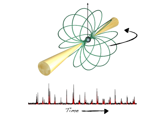
Pulsars are born in supernova explosions of massive stars, created in the collapse of the progenitors core. Unlike most other astrophysical objects, pulsars emit across the whole electromagnetic spectrum (from radio to optical, X- and gamma-rays) at the expense of their rotational energy, i.e., the pulsar spins down as rotational energy is radiated away by its co-rotating magnetic field, a plasma wind, and broadband electromagnetic radiation. Thereby all radiation is powered by rotational energy, which distinguishes pulsars from “accretion powered” neutron stars. With the magnetic axis being inclined to the rotation axis, the pulsar acts like a cosmic light-house emitting a radio pulse that can be detected once per rotation when the beam is directed towards Earth (cf. Fig. 1).

The loss in rotational energy leads to an increase in rotation period, $P$, described by a measured $\dot{P}>0$. Equating the corresponding energy output of the dipole to the loss rate in rotational energy, we obtain an estimate for the magnetic field strength at the pulsar surface. Typical values are of order $10^{12}$ G, although field strengths up to $10^{14}$ G have been observed msk+03 . Millisecond pulsars (MSPs) have lower field strengths of the order of $10^{8}$ to $10^{10}$ G which appear to be a result of their evolutionary history. The evolution can be tracked by two parameters, the observed rotational slow-down, $\dot{P}$, and the resulting evolution in pulsar period, $P$. This is usually done in a (logarithmic) $P$-$\dot{P}$-diagram as shown in Figure 2.

Figure 2: The $P-\dot{P}$–diagram for the known pulsar population. Characteristic age ($\tau=P/2\dot{P}$), surface magnetic field ($B=3.2\times 10^{19}\sqrt{P\dot{P}}$ G) and spin-down luminosity ($\dot{E}=4\pi I\dot{P}/P^{3}$, with $I$ being the moment of inertia) are functions of $P$ and $\dot{P}$ and are hence indicated as lines of corresponding value. Binary pulsars are marked by a circle. The lower solid line represents the pulsar “death line” enclosing the “pulsar graveyard” where pulsars are expected to switch off radio emission. The gray area in the top right corner indicates the region where the surface magnetic field appears to exceed the quantum critical field of $4.4\times 10^{13}$ Gauss. For such values, some theories expect the quenching of radio emission in order to explain the radio-quiet “magnetars” (i.e. Soft-gamma ray repeaters, SGRs, and Anomalous X-ray pulsars, AXPs).

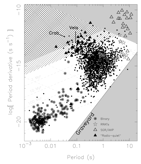
Most known pulsars have spin periods between 0.1 and 1.0 s with period derivatives of typically $\dot{P}=10^{-15}$ s s^-1. Selection effects are only partly responsible for the limited number of pulsars known with very long periods, the longest known period being 8.5 s ymj99 . The dominant effect is due to the “death” of pulsars when their slow-down has reached a critical state. This state seems to depend on a combination of $P$ and $\dot{P}$ known as the pulsar death-line. The normal life of radio pulsars is limited to a few tens or hundreds million years or so.

The described evolution does not explain the over 200 pulsars in the lower left of the $P-\dot{P}$-diagram (Fig. 2). These pulsars have simultaneously small periods (few milliseconds) and small period derivatives ($\dot{P}\leq 10^{-18}$ s s^-1). These millisecond pulsars (MSPs) are much older than ordinary pulsars with ages up to $\sim 10^{10}$ yr. MSPs evolve from pulsars with a binary companion. Once the binary companion evolves and overflows its Roche lobe, it transfers mass and thereby angular momentum (e.g. acrs82 ). In this process, previously “dead” pulsars are recycled to MSPs via an accreting X-ray binary phase. This has a number of observational consequences: a) most normal pulsars do not develop into a MSP as they have long lost a possible companion during their violent birth event; b) for surviving binary systems, X-ray binary pulsars represent the progenitor systems for MSPs; c) the final spin period of recycled pulsars depends on the mass of the initial binary companion. A more massive companion evolves faster, limiting the duration of the accretion process; d) the majority of MSPs have low-mass white-dwarf companions as the remnant of the binary star. These systems evolve from low-mass X-ray binary systems; e) high-mass X-ray binary systems represent the progenitors for double neutron star systems (DNSs). DNSs are rare since these systems need to survive a second supernova explosion. The resulting MSP is only mildly recycled with a period of tens of millisecond. This picture explains the observation that $\sim 80$% of all MSPs are in a binary orbit while this is true for only less than 1% of the non-recycled population. For MSPs with a low-mass white dwarf companion the orbit is nearly circular. In case of DNSs, the orbit is affected by the unpredictable nature of the kick imparted onto the newly born neutron star in the asymmetric supernova explosion of the companion. If the system survives, the result is typically an eccentric orbit with an orbital period of a few hours. However, there is also evidence for the existence of low-kick supernova, producing DNSs with low eccentricity and relatively low-mass neutron star companions (e.g. tlp15 ).

Source with the largest estimated magnetic fields ($\sim 10^{15}$ G), the so called magnetars, are located in the upper right corner of Fig. 2. Here, the observed luminosity appears to exceed the neutron stars’ spin-down energy loss, suggesting that magnetars in addition to the spin-down energy are powered by converting magnetic field energy (see e.g. kk16 for a comparison of magnetars to rotation powered radio pulsars). Only four magnetars have been detected as (transient) radio sources while all appear to be X-ray and gamma-ray sources. The long-term timing is not regular, so that applications as discussed below, are unlikely to be possible.

From timing measurements of binary MSPs (see Section1.2), we can measure neutron star masses. Those are found in a range between about 1.2 and 2$M_{\odot}$ of16 ; ato+16 with the the maximum mass afw+13 ruling out the softest equation-of-sate dpr+10 . The MSP mass distribution is strongly asymmetric. The diversity in spin and orbital properties of high-mass NSs suggests that this is most likely not a result of the recycling process, but rather reflects differences in the NS birth masses. The asymmetry is best accounted for by a bimodal distribution with a low mass component centered at $1.39M_{\odot}$ and a high-mass component with a mean of $1.81M_{\odot}$ ato+16 . These equations-of-state yield radii not too different from the very first calculations by Oppenheimer & Volkov ov39 , i.e. about 20 km in diameter, and are consistent with the blackbody emission radii determined from X-ray observations of16 . This makes neutron stars the most compact objects in the observable Universe.

1.2 Pulsar Timing: pulsars as clocks

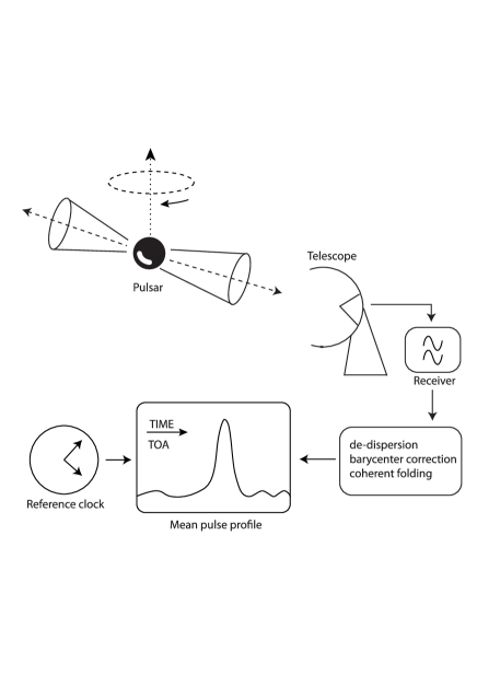
The basic principle of pulsar timing is the measurement of a “time-of-arrival” (TOA) of pulses and their identification with a specific rotation number of the neutron star (cf. Fig. 3).

Figure 3: Typical pulsar detection chain. The pulsar beams sweep across the radio antenna. Radio signals are recorded and analyzed in order to produce a mean pulse profile. The data processing comprises a removal of dispersion effects caused by the interstellar medium (“de-dispersion”), correction for the position and proper motion of the observatory (“barycenter correction”) and coherent folding of many pulses. The time of arrival (TOA) of the pulse peak is measured against a reference clock. (Fig. adapted from D. Lorimer)

The aim is to obtain a “coherent timing solution”, where the term “coherent” refers to a complete description of the rotational phase. The experiment is repeated many times, and the measured TOAs are compared to the prediction of the timing solution. Deviations measured as timing residuals are minimized by an adjustment of the timing parameters. Eventually, the uncertainties in the rotational model are so small, that not only no rotation is missed or mislabeled between observations, but such that the timing model is able to predict the arrival time to microsecond precision or better for observations decades into the future.

Radio pulsars are usually too weak to be detected in their single pulses, so that first an average pulse must be formed to increase the signal-to-noise ratio. Single pulses also usually differ in shape, intensity and exact pulse phase (see Fig. 1), but occur within a well-defined window given by the average pulse shape. Therefore, using an average pulse also improves the timing precision and allows the usage of a technique known as template matching. With the average pulse shape expected to be constant between observations, one can compare the measured pulse form with a high signal-to-noise “template” obtained from the addition of many earlier observations by using a cross-correlation. Assuming that the discretely sampled profile, ${\cal P}(t)$, is a scaled and shifted version of the template, ${\cal T}(t)$, with added noise, ${\cal N}(t)$, we may write

$${\cal P}(t)=a+b{\cal T}(t-\tau)+{\cal N}(t)$$ (1)

where $a$ is an arbitrary offset and $b$ a scaling factor. The time shift between the profile and the template, $\tau$, yields the TOA relative to a fiducial point of the template and the start time of the observation tay92 . Hence, the TOA is thereby defined as the arrival time of the nearest pulse to the mid-point of the observation. The uncertainty of a TOA measurement, $\sigma_{\rm TOA}$ improves with signal-to-noise ratio (hence, size of the used telescope) and sharpness of the pulse features, as this enables a more precise cross-correlation result. For MSPs, a few thousand pulses can be added easily in a few minutes of observing time. This usually results in extremely stable profiles. In addition to their higher rotational stability and short duration pulses, this represents an important factor in explaining the superior timing stability of MSPs when compared to normal pulsars.

By measuring the arrival time of the pulsar signals very precisely, we can study effects that determine the propagation of the pulses in four-dimensional space-time. As indicated, the aim is to determine the rotation number of an observed pulse, counting from some reference epoch, $t_{0}$. We can write

$$N=N_{0}+\nu_{0}\times(t-t_{0})+\frac{1}{2}\dot{\nu}_{0}\times(t-t_{0})^{2}+...,$$ (2)

where $N_{0}$ is the pulse number and $\nu_{0}$ the spin frequency at the reference time, respectively. Whilst for most MSPs a second derivative, $\ddot{\nu}$, is usually too small to be measured, we expect $\nu$ and $\dot{\nu}$ to be related via the physics of the braking process,

$$\dot{\nu}=-\mbox{const.}\times\nu^{n}.$$ (3)

For magnetic dipole braking the braking index takes the value $n=3$. If $\nu$ and its derivatives are accurately known and if $t_{0}$ coincides with the arrival of a pulse, all following pulses should appear at integer values of $N$ — when observed in an inertial reference frame. However, our observing frame is not inertial, as we are using telescopes that are located on a rotating Earth orbiting the Sun. Therefore, we need to transfer the pulse times-of-arrival (TOAs) measured with the observatory clock (topocentric arrival times) to the center of mass of the solar system as the best approximation to an inertial frame available. The transformation of a topocentric TOA to such barycentric arrival times, $t_{\rm SSB}$, is given by

$$t_{\rm SSB}= t_{\rm topo}-t_{0}+t_{\rm corr}-k\times{\rm DM}/f_{\rm obs}^{2}\;,$$ (4)

$$+ \Delta_{{\rm Roemer,}\odot}+\Delta_{{\rm Shapiro,}\odot}+\Delta_{{\rm Einstein,}\odot}\;,$$ (5)

$$+ \Delta_{\rm Roemer,Bin}+\Delta_{\rm Shapiro,Bin}+\Delta_{\rm Einstein,Bin}.$$ (6)

where DM is the so called dispersion measure, representing the integrated path length of free electron along the line of sight, and $f_{\rm obs}$ is the observing radio frequency (see below). We have split the transformation into three lines. The first two lines apply to every pulsar whilst the third line is only applicable to binary pulsars.

Clock and frequency corrections

The observatory time is typically maintained by local Hydrogen-maser clocks monitored by GPS signals. In a process involving a number of steps, clock corrections, $t_{\rm corr}$, are retroactively applied to the arrival times in order to transfer them to a uniform atomic time that would be kept by an ideal atomic clock on the geoid. It is published retroactively by the Bureau International des Poids et Mesures (BIPM).

The free electrons in the interstellar medium interact with the propagation radio signal, causing a frequency dependent group velocity. Consequently, the frequency components of the broadband pulse signal emitted a higher radio frequency $f_{\rm obs}$ arrives earlier than the corresponding low frequency components. Hence, due to this dispersion, the measured arrival time depends on the observing frequency, $f_{\rm obs}$ and the dispersion measure (DM). The TOA is therefore corrected for a pulse arrival at an infinitely high frequency (last term in Eqn. 4). For the best pulsars, the limiting factor in timing precision is often “interstellar weather” that causes small changes in DM and hence time-varying drifts in the TOAs. In those cases, the above term is, for instance, extended to include time-derivatives of DM which can be measured using multi-frequency observations.

Barycentric corrections

The Roemer delay, $\Delta_{{\rm Roemer,}\odot}$, is the classical light-travel time between the phase center of the telescope and the solar system barycenter (SSB). Given a unit vector, $\hat{s}$, pointing from the SSB to the position of the pulsar and the vector connecting the SSB to the observatory, $\vec{r}$, we find:

$$\Delta_{{\rm Roemer,}\odot}=-\frac{1}{c}\;\vec{r}\cdot\hat{s}=-\frac{1}{c}\left(\vec{r}_{\rm SSB}+\vec{r}_{\rm EO}\right)\cdot{\hat{s}}.$$ (7)

Here $c$ is the speed of light and we have split $\vec{r}$ into two parts. The vector $\vec{r}_{\rm SSB}$ points from the SSB to the center of the Earth (geocenter). Computation of this vector requires accurate knowledge of the locations of all major bodies in the solar system and uses solar system ephemerides. The second vector $\vec{r}_{\rm EO}$, connects the geocenter with the phase center of the telescope. In order to compute this vector accurately, the non-uniform rotation of the Earth has to be taken into account, so that the correct relative position of the observatory is derived.

The Shapiro delay, $\Delta_{{\rm Shapiro,}\odot}$, is a relativistic correction that corrects for an extra delay due to the curvature of space-time in the solar system sha64 . It is largest for a signal passing the Sun’s limb ($\sim 120$ $\mu$s) while Jupiter can contribute as much as 200 ns. In principle one has to sum over all bodies in the solar system, but in practice only the Sun is usually taken into account.

The last term in Eqn. 5, $\Delta_{{\rm Einstein,}\odot}$, is called Einstein delay and it describes the combined effect of gravitational redshift and time dilation due to motion of the Earth and other bodies, taking into account the variation of an atomic clock on Earth in the varying gravitational potential as it follows its elliptical orbit around the Sun bh86 .

Relative motion & Shklovskii effect

If the pulsar is moving relative to the SSB, the transverse component of the velocity, $v_{t}$, can be measured as the vector $\hat{s}$ in Eqn. (7) changes with time. Present day timing precision is not sufficient to measure a radial motion although it is theoretically possible. This leaves Doppler corrections to observed periods, masses etc. undetermined. The situation changes if the pulsar has an optically detectable companion such as a white dwarf for which Doppler shifts can be measured from optical spectra.

Another effect arising from a transverse motion is the Shklovskii effect, also known in classical astronomy as secular acceleration. With the pulsar motion, the projected distance of the pulsar to the SSB is increasing, leading to an increase in any observed change of periodicity, such as pulsar spin-down or orbital decay. The observed pulse period derivative, for instance, is increased over the intrinsic value by

$$\left(\frac{\dot{P}}{P}\right)_{\rm obs}=\left(\frac{\dot{P}}{P}\right)_{\rm int}+\frac{1}{c}\;\frac{v_{t}^{2}}{d}.$$ (8)

For MSPs where $\dot{P}_{\rm int}$ is small, a significant fraction of the observed change in period can be due to the Shklovskii effect.

Table 1: Constraining specific (classes of) gravity theories using radio pulsars. See Refs. wex14 ; kk16 for details.

Theory (class)	Method	Ref.
Scalar-tensor gravity:
Jordan-Fierz-Brans-Dicke	limits by PSR J1738+0333 and PSR J0348+0432, comparable to best Solar system test (Cassini)	fwe+12
Quadratic scalar-tensor gravity	for $\beta_{0}<-3$ and $\beta_{0}>0$ best limits from PSR-WD systems, in particular PSR J1738+0333 and PSR J0348+0432	fwe+12
Massive Brans-Dicke	for $m_{\varphi}\sim 10^{-16}$ eV: PSR J1141$-$6545	abwz12
Vector-tensor gravity:
Einstein-Æther	combination of pulsars (PSR J1141$-$6545, PSR J0348+0432, PSR J0737$-$3039, PSR J1738+0333)	ybby14
Hořava gravity	combination of pulsars (see above)	ybby14
TeVeS and TeVeS-like theories:
Bekenstein’s TeVeS	excluded using Double Pulsar	ks+14
TeVeS-like theories	excluded using PSR 1738+0333	fwe+12

Binary pulsars

Equation (4-5) is used to transfer the measured TOAs to the SSB. If the pulsar has a binary companion, the light-travel time across the orbit and further relativistic effects need to be taken into account (see Eqn. 6). That adds additional orbital parameters to the set of timing parameters which have to be solved in the timing process (see below). In the simplest case, five Keplerian parameters need to be determined, i.e. orbital period, $P_{\rm b}$; the projected semi-major axis of the orbit, $x\equiv a\sin i$ where $i$ is the (usually unknown) orbital inclination angle; the orbital eccentricity, $e$; the longitude of periastron, $\omega$; and and the time of periastron passage, $T_{0}$. For a number of binary systems this Keplerian description of the orbit is not sufficient and corrections need to be applied. These can be either time derivatives of Keplerian parameters or parameters describing completely new effects (e.g. those of a Shapiro delay due to curved spacetime near the companion). In any case, it is important to note that we do not have to assume a particular theory of gravity when measuring such relativistic corrections, called “post-Keplerian” (PK) parameters dd85 ; dd86 . Instead, we can take the observational values and compare them with predictions made within a framework of specific theories of gravity dt92 .

In GR, the five most important PK parameters are given by the expressions below rob38 ; bt76 ; dd86 ; pet64 .

$$\dot{\omega} = 3T_{\odot}^{2/3}\left(\frac{P_{\rm b}}{2\pi}\right)^{-5/3}\;\frac{1}{1-e^{2}}\;(M_{p}+M_{c})^{2/3},$$ (9)

$$\gamma = T_{\odot}^{2/3}\left(\frac{P_{\rm b}}{2\pi}\right)^{1/3}\;e\frac{M_{c}(M_{p}+2M_{c})}{(M_{p}+M_{c})^{4/3}},$$ (10)

$$r = T_{\odot}M_{c},$$ (11)

$$s = \sin i=T_{\odot}^{-1/3}\left(\frac{P_{\rm b}}{2\pi}\right)^{-2/3}\;x\;\frac{(M_{p}+M_{c})^{2/3}}{M_{c}},$$ (12)

$$\dot{P}_{\rm b} = -\frac{192\pi}{5}T_{\odot}^{5/3}\left(\frac{P_{\rm b}}{2\pi}\right)^{-5/3}f(e)\frac{M_{p}M_{c}}{(M_{p}+M_{c})^{1/3}},$$ (13)

where all masses are expressed in solar units, $G$ is Newton’s gravitational constant, $c$ the speed of light and

$$f(e)=\frac{\left(1+(73/24)e^{2}+(37/96)e^{4}\right)}{(1-e^{2})^{7/2}}.$$ (14)

$P_{b}$ is the period and $e$ the eccentricity of the binary orbit. The masses $M_{p}$ and $M_{c}$ of pulsar and companion, respectively, are expressed in solar masses ($M_{\odot}$) where we define the constant $T_{\odot}=GM_{\odot}/c^{3}=4.925490947\mu$s. $G$ denotes the Newtonian constant of gravity and $c$ the speed of light.

The first PK parameter, $\dot{\omega}$, describes the relativistic advance of periastron in rad s^-1. It is the easiest to measure for orbits with non-zero eccentricities (note that $\omega$ is only poorly defined for $e\approx 0$ and so is $\dot{\omega}$). From a measurement of $\dot{\omega}$, we obtain from Equation (9) the total mass of the system, $(M_{p}+M_{c})$.

The orbital decay due to gravitational-wave damping is expressed by the (dimensionless) change in orbital period, $\dot{P}_{\rm b}$. Any metric theory of gravity that embodies Lorentz-invariance in its field equations predicts gravitational radiation and, hence, $\dot{P}_{\rm b}$. If a theory satisfies the strong equivalence principle, like GR, gravitational dipole radiation is not expected, but quadrupole emission will be the lowest multipole term. In alternative theories, while the inertial dipole moment may remain uniform, the gravitational wave dipole moment may not, and dipole radiation may be predicted. The magnitude of this effect depends on the difference in gravitational binding energies, expressed by the difference in coupling constants to a scalar gravitational field.

The other two parameters, $r$ and $s$, are related to the Shapiro delay caused by the curvature of space-time due to the gravitational field of the companion. They are measurable, depending on timing precision, if the orbit is seen nearly edge-on.

Obtaining a timing solution

Equations (2) to (6) contain the set of timing parameters that need to be determined. Many of them are not known a priori (or only with limited precision after the discovery of a pulsar) and need to be determined precisely in a least squares fit analysis of the measured TOAs. The parameters can be categorized into three groups: (a) astrometric parameters (i.e. position, proper motion, parallax contained in the Römer and Shapiro delay, respectively); (b) spin parameters (i.e. rotation frequency, $\nu$, and higher derivatives); (c) binary parameters.

Given a minimal set of starting parameters, a least squares fit is needed to match the measured arrival times to pulse numbers according to Equation (2). We minimize the expression

$$\chi^{2}=\sum_{i}\left(\frac{N(t_{i})-n_{i}}{\sigma_{i}}\right)^{2}$$ (15)

where $n_{i}$ is the nearest integer to $N(t_{i})$ and $\sigma_{i}$ is the TOA uncertainty in units of pulse period (turns).

In order to obtain a phase-coherent solution that accounts for every single rotation of the pulsar between two observations, one starts off with a small set of TOAs that were obtained sufficiently close in time so that the accumulated uncertainties in the starting parameters do not exceed one pulse period. Gradually, the data set is expanded, maintaining coherence in phase. When successful, post-fit residuals expressed in pulse phase show a Gaussian distribution around zero with a root mean square that is comparable to the TOA uncertainties. Incorrect or incomplete timing models cause systematic structures in the post-fit residuals identifying the parameter that needs to be included or adjusted. The precision of the parameters improves with length of the data span and the frequency of observation, but also with orbital coverage in the case of binary pulsars.

Table 2: Examples of obtained relative precision using pulsar timing. Corresponding (example) references are cited in the last column.

Clock properties:
Spin frequency	$\mathrel{\hbox{\hbox to0.0pt{\hbox{\lower 4.0pt\hbox{$\sim$}}\hss}\hbox{$<$}}}10^{-15}$	vbv+08
Orbital period	$\mathrel{\hbox{\hbox to0.0pt{\hbox{\lower 4.0pt\hbox{$\sim$}}\hss}\hbox{$<$}}}10^{-11}$	ks+14
Frequency stability	$\mathrel{\hbox{\hbox to0.0pt{\hbox{\lower 4.0pt\hbox{$\sim$}}\hss}\hbox{$<$}}}10^{-15}$	hcm+12
Masses measurements:
Neutron star	$\mathrel{\hbox{\hbox to0.0pt{\hbox{\lower 4.0pt\hbox{$\sim$}}\hss}\hbox{$<$}}}10^{-4}$	wnt10
White dwarf companion	$\mathrel{\hbox{\hbox to0.0pt{\hbox{\lower 4.0pt\hbox{$\sim$}}\hss}\hbox{$<$}}}10^{-3}$	hbo06
Main sequence star companion	$\mathrel{\hbox{\hbox to0.0pt{\hbox{\lower 4.0pt\hbox{$\sim$}}\hss}\hbox{$<$}}}10^{-2}$	fbw+11
Mass of Jupiter and moons	$\mathrel{\hbox{\hbox to0.0pt{\hbox{\lower 4.0pt\hbox{$\sim$}}\hss}\hbox{$<$}}}10^{-6}$	chm+10
Astrometry:
Distance	$\mathrel{\hbox{\hbox to0.0pt{\hbox{\lower 4.0pt\hbox{$\sim$}}\hss}\hbox{$<$}}}10^{-2}$	vbv+08
Proper motion:	$\mathrel{\hbox{\hbox to0.0pt{\hbox{\lower 4.0pt\hbox{$\sim$}}\hss}\hbox{$<$}}}10^{-15}$	vbv+08
Gravity tests:
Test of General Relativity	$\mathrel{\hbox{\hbox to0.0pt{\hbox{\lower 4.0pt\hbox{$\sim$}}\hss}\hbox{$<$}}}10^{-4}$	ks+14
Constancy of grav. constant, $\dot{G}/G$	$\mathrel{\hbox{\hbox to0.0pt{\hbox{\lower 4.0pt\hbox{$\sim$}}\hss}\hbox{$<$}}}10^{-12}$	fwe+12
GW chara. strain $\Delta L/L$	$\mathrel{\hbox{\hbox to0.0pt{\hbox{\lower 4.0pt\hbox{$\sim$}}\hss}\hbox{$<$}}}10^{-16}$	2016MNRAS.458.1267V

1.3 Pulsars as tools

Pulsar combine a number of interesting properties: they are compact objects with strong gravitational fields; they are small enough to essentially act as test masses in binary systems; the act as natural precision clocks; their interior contains the most extreme dense matter in the observable Universe; they emit coherent radio emission that is up to 100% polarised; they are not only radio sources but pulsar emission is often seen across the whole electromagnetic spectrum. There are many more properties that one could list, but just those are sufficient to make pulsars an exciting and useful tool for probing a wide range of physics or for probing the interstellar or other surrounding media. They are especially useful for testing theories of gravity. This can be done either with pulsars as part of a binary system, or also as part of a Galactic-sized detector for low-frequency gravitational waves. We will expand on the latter in more detail below, but concentrate for a moment on binary pulsars.

While, strictly speaking, binary pulsars move in the weak gravitational field of a companion, they do provide precision tests of the (quasi-stationary) strong-field regime. This becomes clear when considering that the majority of alternative theories predicts strong self-field effects which would clearly affect the pulsars’ orbital motion. Hence, tracing their fall in a gravitational potential, we can search for tiny deviations from general relativity, providing us with unique precision strong-field tests of gravity. For instance, in binary systems a wide range of relativistic effects can be observed, identified and studied (e.g. wil14 ), including concepts and principles deeply embedded in theoretical frameworks. If a specific alternative theory is developed sufficiently well, one can also use radio pulsars to test the consistency of this theory. Table 1 summarizes some, where this has been possible. In particular, the radiative properties of a theory are a very powerful and sensitive probe, so that every successful theories has to pass the binary pulsar experiments.

The precision of pulsars allow also applications that may not be directly obvious. One such application is space navigation that we will describe in detail below. Key is the clock-like stability of pulsars taylor1991 ; matsakis1997 , allowing us to make extremely precise measurements. Table 2 gives an idea about the precision of pulsar timing that we achieve today. With larger telescopes being built (e.g. the South African MeerKAT), precision and the number applications will increase. Perhaps, at some point, we will establish a complete pulsar-based timescale.

2 Autonomous Spacecraft Navigation Based On Pulsar Timing

Possible implementations of autonomous navigation systems were already discussed in the early days of space flight battin1964 . In principle, the orbit of a spacecraft can be determined by measuring angles between solar system bodies and astronomical objects; e.g., the angles between the Sun and two distant stars and a third angle between the Sun and a planet. However, because of the limited angular resolution of on-board star trackers and sun sensors, this method yields spacecraft positions with uncertainties that accumulate typically to several thousand kilometers. Alternatively, the navigation fix can be established by observing multiple solar system bodies: It is possible to autonomously triangulate the spacecraft position from images of asteroids taken against a background field of distant stars. This method was realized and flight-tested on NASA’s Deep-Space-1 mission between October 1998 and December 2001. The Autonomous Optical Navigation (AutoNav) system on-board Deep Space 1 provided the spacecraft orbit with $1\sigma$ errors of $\pm 250$ km and $\pm 0.2$ m/s, respectively riedel2000 .

An alternative and very appealing approach to autonomous spacecraft navigation is based on pulsar timing. The idea of using these celestial sources as a natural aid to navigation goes back to the 1970s when Downs downs1974 investigated the idea of using pulsating radio sources for interplanetary navigation. He analyzed a method of position determination by comparing TOAs at the spacecraft with those at a reference location. Within the limitations of technology and pulsar data available at that time (a set of only 27 radio pulsars were considered), Downs showed that spacecraft position errors on the order of 1500 km could be obtained after 24 hours of signal integration. A possible improvement in precision by a factor of 10 was estimated if better (high-gain) radio antennas were available for the observations.

Chester & Butman chester+butman1981 adopted this idea and proposed to use X-ray pulsars, of which about one dozen were known at the time. They estimated that 24 hours of data collection from a small on-board X-ray detector with 0.1 m² collecting area would yield a three-dimensional position accurate to about 150 km. Their analysis, though, was not based on detailed simulations or actual pulsar timing analyses; neither did it take into account the technological requirements or weight and power constraints for implementing such a navigation system.

These early studies on pulsar-based navigation estimated relatively large position and velocity errors so that this method was not considered to be an applicable alternative to the standard navigation schemes. However, pulsar astronomy has improved considerably over the last 40 years since these early proposals. Meanwhile, pulsars have been detected across the electromagnetic spectrum and their emission properties have been studied in great detail (see Section 1). Along with the recent advances in detector and telescope technology this motivates a general reconsideration of the idea of pulsar-based spacecraft navigation.

2.1 The relevance of the various pulsar types for navigation

We already discussed the various types of pulsars, namely rotation-, accretion-, and magnetic-field-powered neutron stars in Section 1. The very complex spin behavior and often unpredictable evolution of rotation period in accretion powered pulsars manifest themselves in erratic changes between spin-up and spin-down as well as X-ray burst activities. This unsteady and non-coherent timing behavior disqualifies them as reference sources for navigation. Similar arguments for magnetars invalidates these sources also for the use in a pulsar-based spacecraft navigation system.

Concerning their application for navigation, the only pulsar class that really qualifies is that of rotation-powered ones. Here, the much higher timing stability of MSPs is of major importance for their use in a pulsar-based navigation system. Of the $\sim 2500$ rotation-powered pulsars known today (Fig. 2), about 150 have been detected in the X-ray band becker2009 , and approximately $1/3$ of them are MSPs. In the past $30-40$ years many of them have been regularly timed with high precision especially in radio observations. Consequently, their ephemerides (RA, DEC, $P$, $\dot{P}$, binary orbit parameters, TOAs and absolute pulse phase for a given epoch, pulsar proper motion etc.) are known with very high accuracy (see Table 2). This is an essential requirement for using these celestial objects as navigation beacons, as it enables us to predict the TOAs of a pulsar for any location in the solar system and beyond.

Figure 4: Iterative determination of position and velocity by a pulsar-based navigation system 2015AN….336..749B .

2.2 Timing irregularities

So far, we have neglected that young rotation-powered pulsars can show glitches in their spin-down behavior, i.e., abrupt increases of rotation frequency, often followed by an exponential relaxation toward the pre-glitch frequency espinoza2011 ; yu2013 . While this is often observed in young pulsars, it is very rarely in old and millisecond pulsars. Nevertheless, the glitch behavior of pulsars has to be taken into account by a pulsar-based navigation system. While it is possible to change the set of pulsars taken as reference when a glitch has been observed, the intrinsic timing noise is a factor which sets a hard limit for the overall accuracy possible for a pulsar-based spacecraft navigator. Timing noise is present in all pulsars, but the level varies between sources. Typical MSPs show timing residuals with an root mean square (RMS) at a level of $\sim 0.1-1\mu$s, which limits the position accuracy then to 30 - 300m.

Figure 5: Measuring the phase difference between the expected and measured pulse peak at an inertial reference location; e.g., the solar system barycenter (SSB). The top profile shows the main pulse peak location as expected at the SSB. The bottom profile is the one measured at a spacecraft and transformed to the SSB by assuming the spacecraft position and velocity during the observation. If the position and velocity assumption was wrong, a phase shift $\Delta\phi$ is observed 2015AN….336..749B .

2.3 Principles of Pulsar-Based Navigation

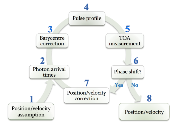
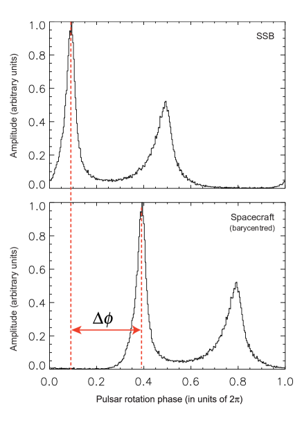
The concept of using pulsars as navigational aids is based on the comparison of measured TOA with predicted TOA at a given epoch and reference location. Figure 3 showed the typical chain for detecting radio signals from a rotation-powered pulsars. For our application here, we perform x-ray observations, where the dedispersion in not necessary. However, the step of applying barycenter correction to the observed photon arrival times (see Section 1.2) is still essential. The pulsar ephemerides along with the position and velocity of the observer are parameters of this correction. Using a spacecraft position that deviates from the true position during the observation results in a phase shift of the pulse peak (or equivalently in a difference in the pulse arrival time). Therefore, the position and velocity of the spacecraft can be adjusted in an iterative process until the pulse arrival time matches with the expected one. The corresponding iteration chain is shown in Figure 4.

Figure 6: Solving the ambiguity problem by observing four pulsars (drawn in two dimensions). The arrows point along the pulsar’s lines-of-sight. Straight lines represent planes of constant pulse phase; black dots indicate intersections of planes 2015AN….336..749B .

An initial assumption of position and velocity is given by the planned orbital parameters of the spacecraft (1). The iteration starts with a pulsar observation, during which the arrival time of individual photons are recorded (2). The photon arrival times have to be corrected for the proper motion of the spacecraft by transforming the arrival times to an inertial reference location; e.g., the solar system barycenter (SSB). As for pulsar observations with terrestrial telescopes, this correction requires knowledge of the (assumed or deduced) spacecraft position and velocity as input parameters. The barycenter corrected photon arrival times allow then the construction of a pulse profile or pulse phase histogram (4) representing the temporal emission characteristics and timing signature of the pulsar. This pulse profile, which is continuously improving in significance during an observation, is permanently correlated with a pulse profile template in order to increase the accuracy of the absolute pulse-phase measurement (see Section 1.2) (5), or equivalently, TOA. From the pulsar ephemeris that includes the information of the absolute pulse phase for a given epoch, the phase difference $\Delta\phi$ between the measured and predicted pulse phase can be determined (cf. Fig. 5).

In this scheme, a phase shift (6) with respect to the absolute pulse phase corresponds to a range difference $\Delta x=cP(\Delta\phi+n)$ along the line of sight toward the observed pulsar. Here, $\Delta\phi$ the phase shift and $n=0,\pm 1,\pm 2,\ldots$ an integer that takes into account the periodicity of the observed pulses. If the phase shift is non-zero, the position and velocity of the spacecraft needs to be corrected accordingly and the next iteration step is taken (7). If the phase shift is zero, or falls below a certain threshold, the position and velocity used during the barycenter correction was correct (8) and corresponds to the actual orbit of the spacecraft.

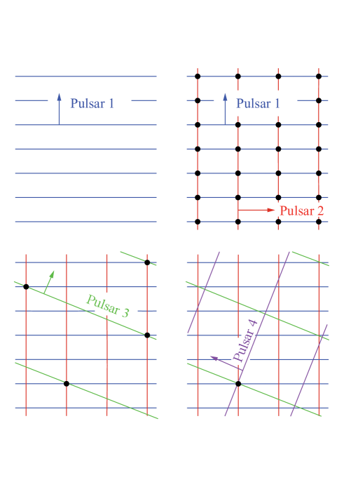
A three-dimensional position fix can be derived from observations of at least three different pulsars (cf. Figure 6). If on-board clock calibration is necessary, the observation of a fourth pulsar is required.

Since the position of the spacecraft is deduced from the phase (or TOA) of a periodic signal, ambiguous solutions may occur. This problem can be solved by constraining the domain of possible solutions to a finite volume around an initial assumed position bernhardt2010 ; bernhardt2011 , or by observing additional pulsars as illustrated in Figure 6.

3 Gravitational Wave Detection Based On Pulsar Timing

3.1 Principles of gravitational wave detection with pulsar timing

Because of their exquisite stability, MSPs also constitute a formidable tool for the detection of low frequency gravitational waves (GWs). The underlying concept is very simple: GWs affect the propagation of radio signals from the pulsar to the Earth, leaving a characteristic signature in the pulses TOAs. If this effect is not included in the timing solutions described in Section 1.2, it will show up in pulsar “$a$” as a residual of the form sv10 :

$$r_{a}(t)=\int_{0}^{t}\frac{\delta\nu_{a}}{\nu_{a}}(t^{\prime})dt^{\prime},$$ (16)

where

$$\frac{\delta\nu_{a}}{\nu_{a}}=\frac{1}{2}\frac{\hat{p}_{a}^{i}\hat{p}_{a}^{j}}{1+\hat{p}_{a}.\hat{\Omega}}\Delta h_{ij}.$$ (17)

Here $\nu_{a}$ is the MSP spin frequency, $\hat{p}_{a}$ denotes the position of the pulsar on the sky, and $\hat{\Omega}$ is the direction of the GW propagation. The quantity

$$\Delta h_{ij}=h_{ij}(t_{a}^{p})-h_{ij}(t)$$ (18)

is the strain of the GW at the location of the pulsar $h_{ij}(t^{p}_{a})$ and on Earth $h_{ij}(t)$ (indices $i,j$ run on the three spatial coordinates), and the pulsar time $t_{a}^{p}$ is related to the Earth time $t$ as:

$$t_{a}^{p}=t-L_{a}(1+\hat{\Omega}.\hat{p}_{a})\equiv t-\tau_{a},$$ (19)

where $L_{a}$ is the distance to the pulsar. In practice, GWs cause drifts in the MSP spin frequency (redshift/blueshift) proportional to the difference of the perturbing field at the pulsar and on Earth. Those drifts cause the pulse to arrive at the Earth earlier/later than expected, resulting in the distinctive timing residual $r_{a}(t)$ of equation (16). The properties of $r_{a}(t)$ ultimately depend on the nature of the perturbation $\Delta h_{ij}$ which can be either a deterministic function or a stochastic process. Both cases are astrophysically relevant, and analysis methods have been developed accordingly.

Pulsars are complex astrophysical objects, governed by largely unknown physics that might affect their intrinsic stability and the GW signal has to be disentangled from a plethora of other effects (see 2015MNRAS.453.2576L for a comprehensive discussion). For example, a deterministic sinusoidal GW signal might be virtually indistinguishable from the effect of a binary companion. Therefore, the GW residual signature needs to be simultaneously detected in several MSPs. This is even more crucial if the GW signal has a stochastic nature. In this case, $r_{a}(t)$ is just a realization of a stochastic process, at par with other stochastic noise sources. GW detection therefore requires the cross correlation of the TOAs from an ensemble of MSPs, forming a pulsar timing array (PTA, 1990ApJ…361..300F ). Three main PTA collaborations are now active in the monitoring of several tens of MSPs: The European Pulsar Timing Array (EPTA 2016MNRAS.458.3341D ), the Parkes Pulsar Timing Array (PPTA 2016MNRAS.455.1751R ) and the North American Nanohertz Observatory for Gravitational Waves (NANOGrav, 2015ApJ…813…65T ). The three collaborations are constantly improving their data, that they also share since 2010 under the aegis of the International Pulsar Timing Array (IPTA, 2016MNRAS.458.1267V ), aiming at the formation of a combined, more sensitive dataset.

Altogether, the three PTAs are timing order of fifty of the best MSPs at a weekly cadence ($\Delta{t}$) for a timespan $T$ of several years (more then 20 for some cases), with a timing precision of few micro-seconds to few tens of nano-seconds. PTAs are therefore sensitive to GWs in the frequency range $1/T<f<1/(2\Delta{t})$, corresponding to few to few-hundred nano-Hertz. Possible GW sources in this frequency range include cosmological stochastic backgrounds from inflation, phase transitions or cosmic strings 2016PhRvX…6a1035L , but the loudest signals are expected from the cosmic population of inspiralling supermassive black hole binaries (SMBHBs) formed following galaxy mergers svc08 .

3.2 Signals from supermassive black hole binaries

In the astrophysically reasonable assumption of circular, monochromatic, non-precessing binary, orbiting at a frequency $f$, the two independent polarization amplitudes generated by the system can be written as sv10 :

$$h_{+}(t) =(1+\cos^{2}\iota)A_{\mathrm{gw}}\cos\Phi(t)\,,$$ (20a)

$$h_{\times}(t) =-2\cos\iota\,A_{\mathrm{gw}}\sin\Phi(t)\,,$$ (20b)

where

$$A_{\mathrm{gw}}(f)=2\frac{{\cal M}^{5/3}}{D}\,\left[\pi f(t)\right]^{2/3}$$ (21)

is the GW amplitude, $D$ the luminosity distance to the GW source, ${\cal M}=(M_{1}M_{2})^{3/5}/(M_{1}+M_{2})^{1/5}$ is the chirp mass (being $M_{1}$ and $M_{2}$ the masses of the two SMBHs) and $\Phi(t)=2\pi\int^{t}f(t^{\prime})dt^{\prime}$ is the GW phase. The metric perturbation in equation (18) can therefore be written as:

$$h_{ij}(t,\hat{\Omega})=e_{ij}^{+}(\hat{\Omega})(h_{+}(t^{p}_{a},\hat{\Omega})-h_{+}(t,\hat{\Omega}))+e_{ij}^{\times}(\hat{\Omega})\,(h_{\times}(t^{p}_{a},\hat{\Omega})-h_{\times}(t,\hat{\Omega})),$$ (22)

where the contribution of both the pulsar and the Earth term have been included. $e_{ij}^{A}(\hat{\Omega})$ ($A=+\,,\times$) are the polarization tensors, that are uniquely defined once one specifies the wave principal axes described by the unit vectors $\hat{m}$ and $\hat{n}$ as,

$$e_{ij}^{+}(\hat{\Omega}) =\hat{m}_{i}\hat{m}_{j}-\hat{n}_{i}\hat{n}_{j}\,,$$ (23a)

$$e_{ij}^{\times}(\hat{\Omega}) =\hat{m}_{i}\hat{n}_{j}+\hat{n}_{i}\hat{m}_{j}\,.$$ (23b)

The signal is therefore deterministic and can be described as $r_{a}(\overrightarrow{\lambda},t)$, where $\overrightarrow{\lambda}$ is the vector of parameters specifying the SMBHB (including SMBH masses, binary sky location, inclination, frequency and initial phase). Note that $r_{a}$ also depends on the sky location of the pulsar through the response function in equation (17) and on the distance to the pulsar that affects the phase and possibly the frequency of the pulsar term (see 2016MNRAS.455.1665B for a full description).

Since galaxy mergers are common, we expect at any time a large population of SMBHB emitting GWs in the PTA band. Therefore, the superposition of many incoherent signals results in a stochastic GW background (GWB), with energy content described in terms of its GW energy density $\rho_{\mathrm{gw}}$ per unit logarithmic frequency, divided by the critical energy density, $\rho_{c}$, to close the Universe:

$$\Omega_{\mathrm{gw}}(f)=\frac{1}{\rho_{c}}\frac{\mathrm{d}\rho_{\mathrm{gw}}}{\mathrm{d}\ln f}=\frac{2\pi^{2}}{3H_{0}^{2}}f^{2}h^{2}_{c}(f).$$ (24)

Here, $f$ is the GW frequency, $\rho_{c}=3H_{0}^{2}/8\pi$ is the critical energy density required to close the Universe, $H_{0}=100~{}h$ km s^-1 Mpc^-1 is the Hubble expansion rate. In the limit of circular GW-driven SMBHBs the ‘characteristic strain’, $h_{c}(f)$, associated with a GWB energy density $\Omega_{\mathrm{gw}}(f)$ is parametrised as a single power-law:

$$h_{c}=A\left(\frac{f}{\mathrm{yr}^{-1}}\right)^{-2/3},$$ (25)

where $A$ is the strain amplitude at a characteristic frequency of 1yr^-1. Finally, $h_{c}$ is directly related to the observable quantity induced by a GWB in the timing residuals, the one-sided power spectral density, $S(f)$, given by:

$$S(f)=\frac{1}{12\pi^{2}}\frac{1}{f^{3}}h_{c}(f)^{2}=\frac{A^{2}}{12\pi^{2}}\left(\frac{f}{\rm{yr}^{-1}}\right)^{-13/3}\rm{yr}^{3}.$$ (26)

Therefore, in the case of a stochastic GWB, the signal is described by a stochastic red process with power spectral density given by equation (26). This can be described by a vector of two parameters $\overrightarrow{\eta}=(A,\gamma)$, where $\gamma=-13/3$ for circular GW-driven SMBHBs. We will see below that this power has a very specific correlations between pairs of pulsars, which is the distinctive signature that has to be searched in PTA data.

3.3 Current status: upper limits from pulsar timing arrays

Whether the signal is deterministic or stochastic, the core aspect of all GW searches is the evaluation of the likelihood that some signal is present in the time series of the pulsar TOAs. Without entering in technical details (see, e.g. 2013MNRAS.428.1147V ; 2015MNRAS.453.2576L ) the likelihood marginalized over the timing parameters can be written as

$$\mathcal{L}(\vec{\theta},\overrightarrow{\lambda},\overrightarrow{\eta}|\overrightarrow{\delta t})=\frac{1}{\sqrt{(2\pi)^{n-m}det(G^{T}CG)}}\times$$

$$\exp{\left(-\frac{1}{2}(\overrightarrow{\delta t}-\overrightarrow{r}(\overrightarrow{\lambda}))^{T}G(G^{T}C(\overrightarrow{\eta})G)^{-1}G^{T}(\overrightarrow{\delta t}-\overrightarrow{r}(\overrightarrow{\lambda}))\right)}.$$ (27)

Here $n$ is the length of the vector $\overrightarrow{\delta t}=\cup\delta{t}_{a}$ obtained by concatenating the individual pulsar TOA series $\delta{t}_{a}$, $m$ is the total number of parameters describing the timing model (see Section 1.2), and the matrix $G$ is related to the design matrix (see 2013MNRAS.428.1147V for details). The variance-covariance matrix $C$, in its more general version, contains contributions from the GWB and from the white and (in general) red noise: $C=C_{gw}(\overrightarrow{\eta})+C_{wn}+C_{rn}$. We refer the reader to 2015MNRAS.453.2576L for exact expressions of the noise variance-covariance matrix.

Likelihoods similar to equation (27) have been used to search for both i) a deterministic single GW sources (e.g., particularly loud SMBHBs rising above the level of the stochastic GWB), or ii) a stochastic GWB.

Figure 7: The 95% upper limit on the gravitational wave strain $A_{\rm gw}$ for the 3 frequentist methods, i.e. ${\cal F}_{p}$ varying noise (Fp), ${\cal F}_{p}$ fixed noise (Fp_ML) and ${\cal F}_{e}$, and the 3 Bayesian methods, i.e. “evolving source” with Earth term only (Bayes_E) and with Earth and Pulsar terms (Bayes_EP) and “non-evolving source” with Earth and Pulsar terms (Bayes_EP_NoEv), performed in the EPTA single source analysis. From 2016MNRAS.455.1665B , where the detailed descriptions of each method can be found.

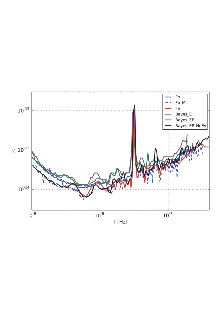
In case i), a deterministic signal $r(\overrightarrow{\lambda},t)$ is added to the model and a search is performed over the parameter space defined by $\overrightarrow{\lambda}$. If the data are better described by noise plus a deterministic signal, then the properties of the latter can be inferred through the posterior distribution of $\overrightarrow{\lambda}$; otherwise, upper limits on the amplitude $A_{\rm gw}$ of a single GW signal (equation (21)) can be placed at every frequency. Searches of this type have been performed by the three major PTAs 2014ApJ…794..141A ; 2014MNRAS.444.3709Z ; 2016MNRAS.455.1665B . The most stringent limit to date has been placed by EPTA and is shown in figure 7 (from 2016MNRAS.455.1665B ) as a function of frequency for different type of searches (see 2016MNRAS.455.1665B for full details). Searches yielded yet no convincing evidence of individual GW sources, and the presence of SMBHBs of few billion solar masses emitting in the PTA range can be ruled out to the distance of the Coma cluster.

Figure 8: From 2016MNRAS.463L…6S . PTA limits on the amplitude of a stochastic GWB. The jagged curves are current PTA sensitivities: EPTA (dot-dashed green), NANOGrav (long-dashed blue), and PPTA (short-dashed red). For each sensitivity curve, stars represent the integrated upper limits to an $f^{-2/3}$ background, and the horizontal ticks are their extrapolation at $f=1$yr^-1, i.e. the upper limit on $A(f=1$yr${}^{-1})$ quoted in the main text. The shaded areas represent the 68% 95% and 99.7% confidence intervals of the characteristic amplitude $h_{c}(f)$ of the expected GWB form SMBHBs. The two panels represent predictions from models employing two different $M_{\rm BH}$”-host bulge mass relations: the one from kh13 (left) and the one from sbs+16 (right). See 2016MNRAS.463L…6S for full details of the employed models.

Figure 9: The recovered correlation between pulsars as a function of angular separation on the sky for a power law noise process in the EPTA analysis. The red and blue lines represent the $68\%$ and $95\%$ confidence intervals for the correlation function when modeled by the lowest 4 Chebyshev polynomials, while the individual points are the mean correlation coefficient with $1\sigma$ uncertainty for each pulsar pair when fitting without assuming a smooth model. The Hellings-Downs correlation is represented by the dotted line. From 2015MNRAS.453.2576L .

In case ii), i.e. the search for a GWB, $C_{gw}(\overrightarrow{\eta})$ is considered in the likelihood evaluation. The signal is stochastic in nature, and has to be singled out among other stochastic sources of noise, including red noise processes peculiar to individual MSPs, correlated noises due to clock or ephemeris errors etc. The smoking gun of a stochastic GWB is provided by the peculiar correlation pattern it introduces in the residuals of pulsar pairs as a function of their separation. This is a general property of any GWB described by the two tensor polarizations allowed by GR and was first worked out by Hellings and Downs hd83 :

$$\Gamma(\zeta_{IJ})=\frac{3}{8}\left[1+\frac{\cos\zeta_{IJ}}{3}+4(1-\cos\zeta_{IJ})\ln\left(\sin\frac{\zeta_{IJ}}{2}\right)\right](1+\delta_{IJ})\,.$$ (28)

Here $\zeta_{IJ}$ is the angle between the pulsars $I$ and $J$ on the sky and $\Gamma(\zeta_{IJ})$ is the overlap reduction function, which represents the expected correlation between the TOAs given an isotropic stochastic GWB, and the $\delta_{IJ}$ term accounts for the pulsar term for the autocorrelation.

In the Fourier representation of the covariance matrix $C_{\rm GW}$, this results in a contribution 2015MNRAS.453.2576L

$$\Psi_{I,J,i,j}=\Gamma(\zeta_{IJ})\varphi^{\mathbf{\mathrm{GWB}}}_{i}\delta_{ij},$$ (29)

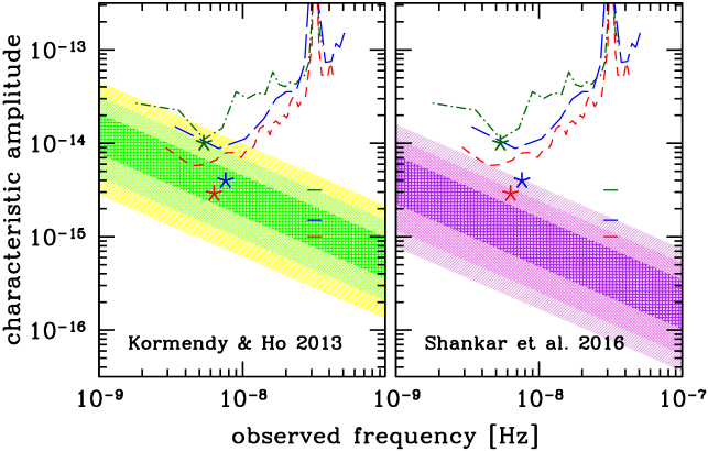
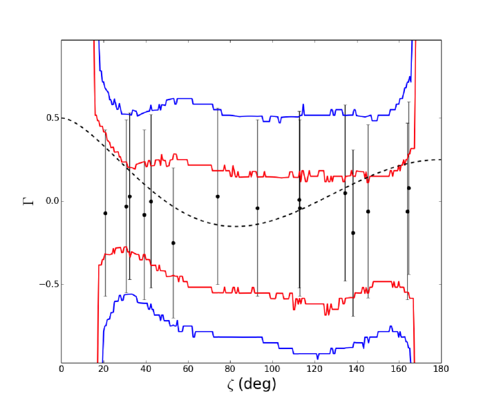
that can be included in the likelihood function (27), appropriately evaluated in the Fourier domain. Lower case indices $i,j$ run over the difference frequency bins of the Fourier decomposition and $\varphi_{i}$ corresponds to the power in the GW signal given by equation (26), evaluated at the central frequency $f_{i}$ if the $i$-th bin. Also in this case, one can evaluate whether the data are better described by including a GWB (and therefore evaluate the vector parameter $\overrightarrow{\eta}$) or not, and in the latter case upper limits on $S_{h}(f)$ (or equivalently on $h_{c}(f)$) can be placed as a factor of frequency. Also in this case, no convincing detection has been made yet. An illustrative example is given in figure 9, from 2015MNRAS.453.2576L , where the measured correlation pattern in the EPTA dataset is shown as a function of the angular separation of the MSP pairs used in the analysis. As expected, the correlation is consistent with zero and the functional form (28) could not be detected. With a null result, limits on $h_{c}(f)$ can be placed, as shown in figure 8 from 2016MNRAS.463L…6S . Upper limits are usually quoted in term of the amplitude $A$ at $f=$yr^-1, as defined in equation (26). Current limits are $A=3\times 10^{-15},1.5\times 10^{-15},10^{-15},1.7\times 10^{-15}$ for EPTA 2015MNRAS.453.2576L , NANOGrav 2016ApJ…821…13A , PPTA 2015Sci…349.1522S and IPTA 2016MNRAS.458.1267V respectively. Note that, although the IPTA limit is not the most stringent one, it has not been obtained combining the most recent individual PTA datasets. Compared to the individual dataset used in the combination, the IPTA limit is a factor of $\approx 2$ better, demonstrating the great potential of collaborating at a worldwide level. As shown in figure 8, these limits start to dig into the level expected by a cosmological population of SMBHBs, and a positive detection might be expected in the near future.

4 Summary and Future Prospects

Pulsars are unique astrophysical sources that combine a number of special properties, which converts them into effective cosmic laboratories for fundamental physics. After having provided the very first evidence for GWs tay94b , pulsars can also be used as GW detectors, probing a nHz-frequency range, where we expect the signals from supermassive binary black holes to occur.

In fact, following galaxy mergers, the SMBHs hosted at their centers pair together forming a binary system. Since galaxy mergers are observed to be frequent in the Universe, a large population of adiabatically inspiralling SMBHBs is expected to fill the nHz GW sky. Such low frequencies are inaccessible to ground and space based GW interferometers, but are in the reach of ongoing and forthcoming PTAs.

Current PTAs are already placing stringent limits to the maximum GW strain emitted by these systems, starting to pierce through the level predicted by current SMBH assembly models. As timing continues, PTA sensitivity naturally increases and progressively extends at lower frequencies (where the signal is expected to be the loudest). Moreover, new instrumentation will play a pivotal role in the coming years. MeerKAT in South Africa and FAST in China will provide even better timing precision on a larger ensemble of pulsars, and by the mid 20s’ we will be surveying thousands of MSPs throughout the galaxy with SKA.

With these premises, it is likely that nHz GW detection will be likely within the next decade, placing another milestone in our understanding of the cosmic evolution of the biggest compact objects in the Universe.

But the clock-like properties of pulsars, and their accessibility across the whole electromagnetic spectrum, also open the door for a wide rage of practical applications. Here we have especially discussed spacecraft navigation.

The knowledge of how to use stars, planets and stellar constellations for navigation was fundamental for mankind in discovering new continents and subduing living space in ancient times. It is fascinating to see how history repeats itself in that a special population of stars may play again a fundamental role in the future of mankind by providing a reference for navigating their spaceships through the Universe.

Autonomous spacecraft navigating with pulsars is feasible when using either phased-array radio antennas of at least 150 m² antenna area or compact light-weighted X-ray telescopes and detectors, which are currently developed for the next generation of X-ray observatories.

Using the X-ray signals from MSPs, Becker et al. 2015AN….336..749B estimated that navigation would be possible with an accuracy of $\pm 5$ km in the solar system and beyond. The uncertainty is dominated by the inaccuracy of the X-ray pulse profile templates that were used for the pulse peak fittings and pulse-TOA measurements. As those are known with much higher accuracy in the radio band, it is possible to increase the accuracy of pulsar navigation down to the meter scale by using radio signals from pulsars for navigation.

The disadvantage of radio observations in a navigation application, though, is the large size and mass of the phased-antenna array. The antenna area is inversely proportional to the square root of the integration time; i.e., the same signal quality can be obtained with a reduced antenna size by increasing the observation time. However, the observing time is limited by the Allen variance of the receiving system and, therefore, cannot become arbitrarily large. In addition, irradiation from the on-board electronics requires an efficient electromagnetic shielding to prevent signal feedback. This shielding will further increase the navigator weight in addition to the weight of the antenna.

The optimal choice of the observing band depends on the boundary conditions given by a specific mission. What power consumption and what navigator weight might be allowed for may determine the choice for a specific wave band.

In general, however, it is clear already today that this navigation technique will find its applications in future astronautics. The technique behind it is very simple and straightforward, and pulsars are available everywhere in the Galaxy. Today $\approx 2500$ pulsars are known. With the next generation of radio observatories, like the SKA, it is expected to detect signals from about 20 000 to 30 000 pulsars smits2009 .

Finally, pulsar-based navigation systems can operate autonomously. This is one of their most important advantages, and is interesting also for current space technologies; e.g., as augmentation of existing GPS/Galileo satellites. Future applications of this autonomous navigation technique might be on planetary exploration missions and on manned missions to Mars or beyond.