Optimized perturbation theory applied to the study of the thermodynamics and BEC-BCS crossover in the three-color Nambu–Jona-Lasinio model

Abstract

The Nambu–Jona-Lasinio model with two flavors, three colors and diquark interactions is analyzed in the context of optimized perturbation theory (OPT). Corrections to the thermodynamical potential that go beyond the large-$N_{c}$ (LN) approximation are taken into account, and the region of the phase diagram corresponding to intermediate chemical potentials and very low temperatures is explored. The simultaneous presence of both the quark-antiquark and diquark condensates can cause the system to behave as a fluid composed of a Bose-Einstein condensate (BEC) or a color superconductor one, in the form of a Bardeen-Cooper-Schrieffer (BCS) superfluid. The BEC-BCS crossover is then studied in the nonperturbative OPT scheme. The results obtained in the context of the OPT method are then contrasted with those obtained in the LN approximation. We show that there are values for the coupling constants related to quark-quark and quark-antiquark interactions where the corrections beyond LN brought by the OPT method can influence the behavior of the diquark condensate and the effective quark mass as a function of the baryon chemical potential. These changes in the behavior of the phase structure of the model modify the location of the critical point related to the phase structure as a whole of the model. Also, when we impose the color neutrality condition, our results show that the nature of the phase transition can change as well, shifting the ratio of the quark-antiquark and quark-quark interactions to higher values in the OPT case as compared to the LN approximation.

I Introduction

Unveiling the phase structure of quantum chromodynamics (QCD) is one active research area today. This is not only because of its intrinsic theoretical interest, but also due to interest across many different fields, ranging from the current heavy-ion collision experiments, to processes able to happen in the astrophysics of compact stellar objects like neutron stars, and also in cosmology. While QCD itself might be considered a well-defined theory, to study its properties deep in the strong coupled nonperturbative regime, like at low temperatures (energies) is notably extremely difficult. Furthermore, when one also tries to study processes at high quark densities (large chemical potential $\mu$), even state-of-the-art numerical techniques, like lattice Monte Carlo QCD simulations (for a recent review, see, e.g., Ref. Ding:2015ona and references therein), one faces tremendous difficulties due to the so-called “sign problem” (associated with the calculation of the determinant of the quarks matrix, which takes on a complex value when $\mu\neq 0$), and progress in this direction has been painfully slow Cristoforetti:2012su ; Fujii:2013sra . As an alternative to bypass the above mentioned difficulties, one typically recourses to low-energy effective models for quantum chromodynamics (QCD), like for example the Nambu–Jona-Lasinio (NJL) type of models KLEVAN ; BUBA , which are valuable tools widely used to try to understand the underlying phase structure of QCD, otherwise unaccessible either through the direct QCD Lagrangian density or lattice QCD techniques.

Of particular interest is the region of the QCD phase diagram at low temperatures and intermediate chemical potentials, even though there is still no consensus on the exact phase in which the quark matter is expected to be found in this region. It corresponds to a portion of the phase diagram not able to be probed by standard methods in QCD, lattice QCD, or through current experiments on particle accelerators. From the point of view of astrophysics, it is estimated that in the cores of so-called compact stars, these conditions are present SCHIMITT . This then strongly motivates studies towards the understanding of the physics in this region of the phase diagram, sometimes also called the region of dense and cold matter, through the use of effective low-energy models that contain characteristics common to QCD, and which highlight some of the expected and relevant behaviors for the system in that region.

One of the most exciting possibilities is the occurrence of quark Cooper pairing (color superconductivity) in this region of cold and dense quark matter, a possibility that has been considered already in Ref. Collins:1974ky , and whose idea has gained considerable interest since then (see, e.g., Ref. Alford:2007xm for a detailed review on this subject). In addition, many works have considered the possibility the transition at low temperature and baryon densities, going from the chiral broken phase to a color superconducting phase at large densities, could proceed through an intermediary phase. In this intermediate phase, the quark matter would undergo a crossover between a regime where diquark pairs form difermion molecules, giving origin then to a Bose-Einstein condensation (BEC), and a weakly coupled Bardeen-Cooper-Schrieffer (BCS) superfluid phase Abuki:2001be ; HUANG1 ; RATTI ; EBERTKLIM ; CHATTER ; NISHABUK ; He:2007kd ; ABUKBRAU ; He:2010nb (for a recent review, see, e.g., Ref. He:2013gga ).

Typically, we can employ an extended NJL model, where besides the usual quark-antiquark four-Fermi interaction, which is responsible for the formation of the chiral condensate of quark-antiquark pairs, a four-Fermi interaction for quark-quark, making possible the formation of diquark condensates, akin to the pairing mechanism in the BCS theory, as the magnitude of this coupling is increased. We can then study the combined competition between these two types of condensates in the system, the chiral and diquark ones. Several works (see, e.g., Refs. HUANG1 ; RATTI ; EBERTKLIM ; He:2010nb ) show that it is possible for the condensate of diquarks initially to form a BEC phase, before the system goes to the BCS state, as we increase the baryon chemical potential going through this BEC-BCS crossover NISHABUK ; ABUKBRAU ; CHATTER . Some possible observational signatures for the BCS regime and the possibility of coexistence of the chiral and diquark phases have been explored in the literature Kitazawa:2002bc , while a connection with high-temperature superconductors and a possible pseudogap was studied in Refs. Kitazawa:2001ft ; Kitazawa:2003cs .

We should note that the NJL model, since it does not include gluon degrees of freedom and thus cannot be used to study confinement, finds applications in the low-energy (temperature) regime of QCD and quark matter, where the gluon degrees of freedom and their effects, e.g., in the physics of (de)confinement, become less relevant. But this low-energy regime corresponds exactly to the regime where the strong coupling and nonperturbative nature of the nuclear matter is relevant, which then likewise requires the use of appropriate nonperturbative methods. The use of the NJL and similar models, as far as the studies in this context are concerned, have mainly focused on the use of the large-$N_{c}$ (LN) method (where $N_{c}$ is the number of colors), or the Hartree approximation BUBA . In practice, the LN method consists of making the change $G\rightarrow\lambda/(2N_{c})$ in the four-Fermi quark-antiquark coupling constant of the model, by keeping $\lambda$ fixed while making $N_{c}$ large and then keeping only the leading term in the expansion when taking $N_{c}\to\infty$, even though we take $N_{c}=3$ at the very end for practical calculations. However, such a method cannot predict physical phenomena that might eventually be related to terms of the next order in $1/N_{c}$ in the expansion, which have to be analyzed through some other self-consistent method and that are required if we want to improve the precision of the results. Even though other approaches have been employed to obtain the thermodynamic potential going beyond the leading LN result to study the phase structure of QCD in the context of the NJL model, these other methods can quickly become more involved or add further free parameters in the analysis (let us recall that with the NJL model, being a nonrenormalizable model, introducing higher-order corrections to the leading-order thermodynamic potential is usually accompanied by the addition of extra renormalization parameters), which is not always welcome.

In this work, we will make use of the OPT method (for a long, but still far from complete, list of past applications of the OPT method in quantum field theory problems, see e.g., Refs. opt1 ; Stevenson:1981vj ; Okopinska:1987hp ; opt2 ; opt4 ; opt5 ; opt6 ; Pinto:1999py ; Pinto:1999pg ; FARIASOPT ; opt8 ). In particular, let us mention that the OPT method has very successfully been applied to NJL-similar types of models in low dimensions, in particular in the Gross-Neveu models in 2+1 dimensions Kneur:2006ht , revealing novel properties in the phase diagram in that context e.g., a tricritical point, not accessed by previous methods. Recent work on the OPT method tries to combine its properties also with those of the renormalization group to further push its applicability as far as renormalization properties are concerned Kneur:2013coa ; Kneur:2015moa ; Kneur:2015uha .

Previous applications of the OPT method for the study of the phase structure in effective models of QCD include, for example, its use in Walecka-type models Krein:1995rp , in the linear sigma model Khan:2016exa ; opt10 ; opt11 , and also in the $SU(2)$ NJL model RUDOPT , whose work in particular we will follow here closely, but in the context of the NJL model with diquark interactions. As already mentioned, with the use of the NJL model, we can only hope to capture some of the low-energy features of QCD at a qualitative level. Given its nonrenormalizability and the other shortcomings already mentioned above, the model itself is not a controlled approximation to QCD. Yet, it is still a valuable tool, in particular to test different methods that can improve over the simpler approximations used in the literature. This is in particular true when considering the NJL in the context of the OPT approximation. By going beyond the simple mean field theory, or LN approximation, the OPT at first order in its implementation already includes some relevant mesonic fluctuations and, in the present work, also contributions from the diquark interaction, which are absent in the LN approximation and which would appear only at the next-to-leading order in an expansion in $1/N_{c}$. In a way, we hope that by including these additional contributions lacking in the LN case, we can improve the applicability of the NJL. At the same time, we can also determine how the inclusion of these corrections performs as compared to the LN approximation and determine whether they can provide both qualitatively and quantitatively relevant corrections beyond the LN case that can be relevant for QCD. The aim of the present work is to present a detailed understanding of the BEC-BCS crossover, making use of the nonperturbative OPT method and applying it to the NJL model endowed with diquark interactions. We will analyze both the cases of absence and presence of color neutrality, and we will use parameters such that a comparison with previous results obtained within the LN method in particular, those obtained by the authors of Ref. SUNHE can be made.

This work is organized as follows: In Sec. II, we briefly introduce the NJL model with diquark interactions. In Sec. III, we explain the OPT scheme and how it is applied to the present. In Sec. IV, we present the derivation of the effective potential for the model and the relevant equations. In Sec. V, we discuss the determination of the parameters of the model and the modifications required when applying the OPT scheme. In Sec. VI, we perform our numerical analysis of the BEC-BCS crossover, and the results obtained in the context of the OPT are contrasted with those obtained in the LN approximation. In Sec. VII, we present our conclusions. An Appendix is included showing some of the technical details required in the determination of the model parameters.

II The NJL with diquark interactions

In this work, we will consider the NJL model with two flavors and three colors ($N_{c}=3$) that includes both the usual chiral four-Fermi quark-antiquark interaction and also the diquark channel, with the Lagrangian density then given by SUNHE ; Kitazawa:2007zs ; HUANG2 ; EBERTKLIM2 ; EBERTKLIM3

$$\mathcal{L} = \bar{\psi}\left(i\gamma^{\mu}\partial_{\mu}-m\right)\psi$$ (1)

$$+ G_{s}\left[\left(\bar{\psi}\psi\right)^{2}+\left(\bar{\psi}i\gamma^{5}\vec{\tau}\psi\right)^{2}\right]$$

$$+ \!\!\!\!\!\!\sum_{a=2,5,7}\!\!\!\!G_{d}\left[\left(\bar{\psi}i\gamma^{5}\tau_{2}\lambda_{a}C\bar{\psi}^{T}\right)\left(\psi^{T}i\gamma^{5}\tau_{2}\lambda_{a}C\psi\right)\right],$$

where $\psi$ represents the quark fields with a flavor doublet $(u,d)$ and color triplet ($N_{c}=3$), as well as a four-component Dirac spinor. In Eq. (1), $\vec{\tau}=(\tau_{1},\tau_{2},\tau_{3})$ and $\lambda_{a}$ are the Pauli and Gell-Mann matrices in the flavor and color spaces, respectively. $C\equiv i\gamma^{2}\gamma^{0}$ is the charge conjugation operator, and $\psi^{T}$ is the transposed quark field. The mass $m$ is the current quark mass, while $G_{s}$ and $G_{d}$ are the coupling constants for quark-antiquark and quark-quark interactions, respectively. In principle, these coupling constants, if followed from the QCD one-gluon exchange approximation and from the Fierz transformation RATTI ; HUANG2 , would be related like $G_{d}=N_{c}/(N_{c}-1)G_{s}/2$, such that for $N_{c}=3$, then $G_{d}=3G_{s}/4$. Here, however, we follow the philosophy of Refs. SUNHE ; EBERTKLIM , where these couplings are treated as free parameters and we will not fix relations between them. In practice, as we will see later on when studying the numerical results, there will always be a ratio of couplings $G_{d}/G_{s}$ below a certain minimum value such that the transition from the chiral phase to the diquarks with a nonvanishing vacuum expectation value will tend to be first order, thus preventing a BEC phase, while for larger values of the ratio there will be a maximum value for this ratio beyond which diquarks would already condense at a baryonic chemical potential $\mu_{B}=0$ i.e., the diquarks would become massless and the vacuum unstable EBERTKLIM3 ; ZHUANG . We will discuss theses issues in more detail later on in the text .

By making use of a Hubbard-Stratonovich transformation in Eq. (1), the four-Fermi interactions can be rewritten in terms of bosonic fields, given by $\zeta$, $\vec{\pi}$, $\phi_{a}$, and $\phi^{*}_{a}$, and can be expressed in the form

$$\mathcal{L}_{B} = \bar{\psi}\left[i\gamma^{\mu}\partial_{\mu}-m-(\zeta+i\gamma^{5}\vec{\pi}\cdot\vec{\tau})\right]\psi+\frac{1}{2}\sum_{a=2,5,7}\psi^{T}\phi_{a}^{*}i\gamma^{5}\tau_{2}\lambda_{a}C\psi$$ (2)

$$+ \frac{1}{2}\sum_{a=2,5,7}\bar{\psi}\phi_{a}i\gamma^{5}\tau_{2}\lambda_{a}C\bar{\psi}^{T}-\frac{1}{4G_{s}}\left(\zeta^{2}+\vec{\pi}^{2}\right)-\frac{1}{4G_{d}}\sum_{a=2,5,7}|\phi_{a}|^{2}.$$

From the use of the Euler-Lagrange equations for $\zeta$, $\vec{\pi}$, $\phi_{a}$, and $\phi^{*}_{a}$, we have that

$$\zeta=-2G_{s}\bar{\psi}\psi,$$ (3)

$$\vec{\pi}=-2G_{s}\bar{\psi}i\gamma^{5}\vec{\tau}\psi,$$ (4)

$$\phi_{a}=2G_{d}\psi^{T}Ci\gamma^{5}\tau_{2}\lambda_{a}\psi,$$ (5)

$$\phi^{*}_{a}=-2G_{d}\bar{\psi}i\gamma^{5}\tau_{2}\lambda_{a}C\bar{\psi}^{T},$$ (6)

and upon substitution in Eq. (2), we recover the original Lagrangian density of Eq. (1).

We will consider, without loss of generality (see, for instance, Ref. SUNHE ), that only the quarks with colors 1 and 2 form diquarks. This condition is satisfied when $\phi_{2}=\phi$ and $\phi_{5}=\phi_{7}=0$. Therefore, we can write the Lagrangian density (2) in the form

$$\mathcal{L}_{B} = \bar{q}_{3}\left[i\gamma^{\mu}\partial_{\mu}-m-(\zeta+i\gamma^{5}\vec{\pi}\cdot\vec{\tau})\right]q_{3}+\bar{q}_{1,2}\left[i\gamma^{\mu}\partial_{\mu}-m-(\zeta+i\gamma^{5}\vec{\pi}\cdot\vec{\tau})\right]q_{1,2}$$ (7)

$$+ \frac{\phi^{*}}{2}q_{1,2}^{T}iC\gamma^{5}\tau_{2}t_{2}q_{1,2}+\frac{\phi}{2}\bar{q}_{1,2}i\gamma^{5}C\tau_{2}t_{2}\bar{q}_{1,2}^{T}-\frac{1}{4G_{s}}\left(\zeta^{2}+\vec{\pi}^{2}\right)-\frac{1}{4G_{d}}|\phi|^{2},$$

where we have used

$$\psi^{T}\equiv\begin{pmatrix}q_{1,2}^{T}&q_{3}^{T}\end{pmatrix}\qquad q_{1,2}^{T}\equiv\begin{pmatrix}q_{1}^{T}&q_{2}^{T}\end{pmatrix},$$ (8)

with $q_{i}$ ($i=1,2,3$) representing the color quark fields and $t_{2}$ being the second Pauli matrix in the color space 1 and 2 (green and red). This form of Eq. (7) makes explicit the fact that quarks with color 3 (blue) do not participate in the formation of the diquark condensate.

III The OPT applied to the NJL model with diquarks

The OPT method consists of initially defining an interpolated (or deformed) Lagrangian density in the form

$$\mathcal{L}_{\delta} \equiv \delta\mathcal{L}+(1-\delta)\mathcal{L}_{0}(\eta_{i})$$ (9)

$$= \mathcal{L}_{0}(\eta_{i})+\delta\left[\mathcal{L}-\mathcal{L}_{0}(\eta_{i})\right],$$

where $\mathcal{L}_{0}$ is the Lagrangian density of a solvable theory, modified by the introduction of arbitrary parameters (which in the present model will be associated with the interaction channels between fermions and their condensates) with mass dimension terms $\eta_{i}$, and $\delta$ is a (bookkeeping) parameter that is used to enable a perturbative expansion; it is set to $\delta=1$ at the end. We can note that if $\delta=1$, we then immediately recover the Lagrangian density of the original theory; if $\delta=0$, we have the solvable Lagrangian density $\mathcal{L}_{0}$. Any physical quantity $\mathcal{P}_{n}$ that is calculated up to a given order $n$ in $\delta$ will, however, depend explicitly on the parameters $\eta_{i}$, which are not part of the original theory. Thus, we must impose an appropriate condition that best fixes the values for these arbitrary parameters in a self-consistent way. The criterion we will use in this work, which was also used in many other previous OPT applications (for other alternative optimization criteria, see, e.g., Refs. opt6 ; FARIASOPT ), is the principle of minimum sensitivity (PMS), by requiring that Stevenson:1981vj

$$\left.\frac{\partial\mathcal{P}_{n}}{\partial\eta_{i}}\right|_{\eta_{i}=\bar{\eta}_{i}}=0,$$ (10)

through which the parameters $\bar{\eta}_{i}$ are those that make the computed quantities an extremum (a minimum) with respect to these mass parameters and guarantee that $\mathcal{P}_{n}$ is locally independent (sensitive) of $\bar{\eta}_{i}$. The convergence of the OPT under different contexts has been shown in the many papers cited in Ref. opt6 .

The interpolation in the present model is performed as follows: Starting from the Lagrangian density in terms of the auxiliary fields, Eq. (2), and following, e.g., the procedure shown in Ref. RUDOPT , we can define the OPT Lagrangian density $\mathcal{L}_{0}$ in Eq. (9) as

$$\!\!\!\!\!\!\!\mathcal{L}_{0} \equiv \bar{\psi}\left(i\gamma^{\mu}\partial_{\mu}-m\right)\psi-\bar{\psi}(\eta+i\gamma^{5}\vec{\tau}\cdot\vec{\eta}_{\pi})\psi$$ (11)

$$- \!\!\!\!\!\!\!\sum_{a=2,5,7}\!\!\!\!\left(\bar{\psi}i\gamma^{5}\tau_{2}\lambda_{a}C\alpha_{1a}^{\prime}\bar{\psi}^{T}\!+\!\psi^{T}i\gamma^{5}\tau_{2}\lambda_{a}C\alpha_{2a}^{\prime}\psi\right).$$

In Eq. (11), the OPT mass parameters $\eta$ and $\eta_{\pi}$ are the ones related to the scalar and pseudoscalar channels, respectively, while $\alpha_{1a}^{\prime}$ and $\alpha_{2a}^{\prime}$ are those for the quark-quark interaction scalar channel. Since $\langle\vec{\pi}\rangle=0$, we can then set $\vec{\eta}_{\pi}=0$ consistently RUDOPT .

Overall, the interpolated Lagrangian density used in the OPT scheme in the present model can then be expressed in the form

$$\mathcal{L}_{\delta,B} = -\delta\frac{(\zeta^{2}+\vec{\pi}^{2})}{4G_{s}}-\delta\frac{|\phi|^{2}}{4G_{d}}+\bar{\psi}\left[i\gamma^{\mu}\partial_{\mu}-m-\delta\left(\zeta+i\gamma^{5}\vec{\tau}\cdot\vec{\pi}\right)-(1-\delta)\eta\right]\psi$$ (12)

$$+ \psi^{T}Ci\gamma^{5}\tau_{2}\frac{\lambda_{2}}{2}\left[\delta\phi^{*}+(1-\delta)\alpha_{2}\right]\psi+\bar{\psi}i\gamma^{5}\tau_{2}\frac{\lambda_{2}}{2}C\left[\delta\phi+(1-\delta)\alpha_{1}\right]\bar{\psi}^{T}\ ,$$

in which we have defined $\alpha_{1}\equiv-2\alpha_{12}^{\prime}$ and $\alpha_{2}\equiv-2\alpha_{22}^{\prime}$, and we have also again performed the rotation $\phi_{2}\equiv\phi$ and $\phi_{5}=\phi_{7}=0$, resulting in $\alpha_{1k}=\alpha_{2k}=0$, with $k=5,7$. It is important to note that when $\delta=1$, we retrieve the original theory given by Eq. (2). We can also conveniently rewrite Eq. (12) as

$$\mathcal{L}_{\delta,B} = \bar{q}_{3}\left[i\gamma^{\mu}\partial_{\mu}-m-\delta(\zeta+i\gamma^{5}\vec{\pi}\cdot\vec{\tau})-(1-\delta)\eta\right]q_{3}+\bar{q}_{1,2}\left[i\gamma^{\mu}\partial_{\mu}-m-\delta(\zeta+i\gamma^{5}\vec{\pi}\cdot\vec{\tau})-(1-\delta)\eta\right]q_{1,2}$$

$$+ \frac{1}{2}q_{1,2}^{T}iC\gamma^{5}\tau_{2}t_{2}\left[\delta\phi^{*}+(1-\delta)\alpha_{2}\right]q_{1,2}+\frac{1}{2}\bar{q}_{1,2}i\gamma^{5}C\tau_{2}t_{2}\left[\delta\phi+(1-\delta)\alpha_{1}\right]\bar{q}_{1,2}^{T}-\frac{\delta}{4G_{s}}\left(\zeta^{2}+\vec{\pi}^{2}\right)-\frac{\delta}{4G_{d}}|\phi|^{2}.$$

IV The effective potential in the OPT method

We are now in position to derive the thermodynamic effective potential for the NJL model with diquark interactions within the OPT scheme. We evaluate the effective potential up to order $\delta^{1}$ in the OPT method, which will by itself already supply us with correction terms going beyond the standard LN approximation.

All relevant Feynman rules regarding the propagators and vertices within the OPT scheme are represented in Fig. 1.

Figure 1: The representation of the Feynman rule elements in the OPT method. (a) Fermionic propagator related to the $\delta$-dependent quark $\Psi$-field. (b) Fermionic propagator when $\delta=0$. (c) Propagator related to the boson (auxiliary) $\zeta$-field. (d) Propagator related to each of three $\pi_{i}$-fields. (e) Propagator related to the diquark auxiliary field, real component $\phi_{R}$. (f) Propagator related to the diquark auxiliary field, imaginary component $\phi_{I}$. (g), (h), (i), (j), The vertices related to the point interactions between a bosonic and two fermionic fields at $\delta=0$. (If fermionic propagators depend on $\delta$, the lines are represented here as thick ones.)

Up to order $\delta$ in the OPT, we will have both one-loop terms, as shown in Fig. 2, and also two-loop terms, as shown in Fig. 3.

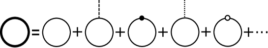
Figure 2: One-loop diagrams in OPT expanded up to order $\delta^{1}$. The thick continuous line represents the fermionic propagator as a function of $\delta$. Thin lines represent the propagator when $\delta=0$. The dashed line represents the $\sigma$-field propagator, while the dotted one is associated with the $\Delta$-field propagator. The large black dot represents a $\delta\eta$-vertex insertion, and the white one represents a $\delta\alpha$-vertex insertion.

Figure 3: To the left of the equality, the sum of two-loop diagrams in OPT ($\propto 1/N_{c}^{1}$) capable of generating contributions of order $\delta^{1}$. To the right of the equality, sum of two-loops diagrams when expanded up to order $\delta^{1}$. All elements are defined according to the legend of Fig. 1.

Below, we will evaluate separately the one-loop and two-loop contributions shown in Figs. 2 and 3, respectively.

IV.1 The one-loop contribution to the effective potential in the OPT expansion

At order $\delta$, the one-loop Feynman’ diagrams contribution to the effective potential in the OPT is shown in Fig. 2. In Fig. 2, a full line is associated with a fermionic propagator related to all quarks, and it is a function of $\delta$. By expanding it in powers of $\delta$ and truncating to ${\cal O}(\delta^{1})$, we obtain the resulting contributions shown on the right-hand side of Fig. 2. The effective potential can be obtained by the usual functional integral technique most easily when one makes use of the standard Nambu-Gor’kov formalism gorkov ; Nambu:1960tm applied to the quark fields. By also using the Matsubara formalism of finite-temperature quantum field theory kapusta and performing the sum over the Matsubara frequencies for the fermions, the obtained effective potential at one loop and order $\delta$ at finite temperature ($T=1/\beta$) and chemical potential can be expressed explicitly in the form

$$V_{{\rm eff};1-{\rm loop},\delta^{1}}^{\mu,\mu_{b},\beta} = \delta\frac{\sigma^{2}}{4G_{s}}+\delta\frac{|\Delta|^{2}}{4G_{d}}$$ (14)

$$- {\cal N}\int{\frac{d^{3}p}{(2\pi)^{3}}\left\{\left[E_{\alpha\vec{p}}^{-}(\mu)+E_{\alpha\vec{p}}^{+}(\mu)\right]+\delta\left[\frac{d}{d\delta}E_{\alpha\vec{p}}^{\delta-}(\mu)+\frac{d}{d\delta}E_{\alpha\vec{p}}^{\delta+}(\mu)\right]_{\delta=0}\right\}}$$

$$- N_{f}\int\frac{d^{3}p}{(2\pi)^{3}}\left\{\left[E_{\vec{p}}^{-}(\mu_{b})+E_{\vec{p}}^{+}(\mu_{b})\right]+\delta\left[\frac{d}{d\delta}E_{\vec{p}}^{\delta-}(\mu_{b})+\frac{d}{d\delta}E_{\vec{p}}^{\delta+}(\mu_{b})\right]_{\delta=0}\right\}$$

$$- 2{\cal N}\int\frac{d^{3}p}{(2\pi)^{3}}\left\{\frac{1}{\beta}\ln{\left(1+e^{-\beta E_{\alpha\vec{p}}^{-}(\mu)}\right)}+\frac{1}{\beta}\ln{\left(1+e^{-\beta E_{\alpha\vec{p}}^{+}(\mu)}\right)}\right.$$

$$- \left.\delta\left[\frac{1}{e^{\beta E_{\alpha\vec{p}}^{\delta-}(\mu)}+1}\frac{d}{d\delta}E_{\alpha\vec{p}}^{\delta-}(\mu)+\frac{1}{e^{\beta E_{\alpha\vec{p}}^{\delta+}(\mu)}+1}\frac{d}{d\delta}E_{\alpha\vec{p}}^{\delta+}(\mu)\right]_{\delta=0}\right\}$$

$$- 2N_{f}\int\frac{d^{3}p}{(2\pi)^{3}}\left\{\frac{1}{\beta}\ln{\left(1+e^{-\beta E_{\vec{p}}^{-}(\mu_{b})}\right)}+\frac{1}{\beta}\ln{\left(1+e^{-\beta E_{\vec{p}}^{+}(\mu_{b})}\right)}\right.$$

$$- \left.\delta\left[\frac{1}{e^{\beta E_{\vec{p}}^{\delta-}(\mu_{b})}+1}\frac{d}{d\delta}E_{\vec{p}}^{\delta-}(\mu_{b})+\frac{1}{e^{\beta E_{\vec{p}}^{\delta+}(\mu_{b})}+1}\frac{d}{d\delta}E_{\vec{p}}^{\delta+}(\mu_{b})\right]_{\delta=0}\right\},$$

where we have defined ${\cal N}\equiv(N_{c}-1)N_{f}$ and

$$\!\!\!E_{\alpha\vec{p}}^{\delta\pm}(\mu^{\prime})\!=\!\sqrt{[E_{\vec{p}}^{\delta\pm}(\mu^{\prime})]^{2}+\prod_{s=1}^{2}[\alpha_{s}+\delta(\Delta_{s}-\alpha_{s})]},$$ (15)

$$E_{\vec{p}}^{\delta\pm}(\mu^{\prime})=E_{\vec{p}}^{\delta}\pm\mu^{\prime},$$ (16)

$$E_{\vec{p}}^{\delta}=\sqrt{\vec{p}^{2}+[M^{\prime}_{\eta}(\delta,\sigma,0)]^{2}},$$ (17)

with $\mu^{\prime}=\mu,\mu_{b}$ and

$$M^{\prime}_{\eta}(\delta,\sigma,0) \equiv M^{\prime}_{\eta}(\delta,\langle\zeta\rangle,\langle\vec{\pi}\rangle)$$ (18)

$$= m+\delta(\langle\zeta\rangle+i\gamma^{5}\langle\vec{\pi}\rangle\cdot\vec{\tau})+(1-\delta)\eta$$

$$= m+\eta+\delta(\sigma-\eta),$$

where we have used $\langle\zeta\rangle=\sigma$ and $\langle\vec{\pi}\rangle=0$. Note that the chemical potentials were included by the usual prescription $i\partial_{0}\rightarrow i\partial_{0}+\mu_{j}$ in Eq. (LABEL:LBfinaldelta), with $\mu_{1}\equiv\mu_{r}$, $\mu_{2}\equiv\mu_{g}$ and $\mu_{3}\equiv\mu_{b}$, but in order to ensure that $SU(2)$ color symmetry between red and green quarks is not explicitly broken, we take $\mu_{g}=\mu_{r}\equiv\mu$. In addition, we have that $\Delta_{1}\equiv\Delta$, $\Delta_{2}\equiv\Delta^{*}$, with $\langle\phi\rangle=\Delta$ and $\langle\phi^{*}\rangle=\Delta^{*}$. (Without loss of generality, we will assume $\Delta^{*}=\Delta$ and $\alpha_{1}=\alpha_{2}\equiv\alpha$, since only the absolute values of these quantities appear at the end.)

Then, in Eq. (14), we have that

$$\left.\frac{d}{d\delta}E_{\vec{p}}^{\delta\pm}(\mu^{\prime})\right|_{\delta=0} = \frac{(m+\eta)(\sigma-\eta)}{E_{\vec{p}}},$$ (19)

$$\left.\frac{d}{d\delta}E_{\alpha\vec{p}}^{\delta\pm}(\mu^{\prime})\right|_{\delta=0} = \frac{1}{E_{\alpha\vec{p}}^{\pm}(\mu^{\prime})}\left[\frac{E_{\vec{p}}^{\pm}(\mu^{\prime})}{E_{\vec{p}}}(m+\eta)(\sigma-\eta)\right.$$ (20)

$$+ \left.\alpha(\Delta-\alpha)\vphantom{\frac{E_{\vec{p}}^{i\pm}(0)}{E_{\vec{p}}(0)}}\right],$$

with

$$E_{\alpha\vec{p}}^{\pm}(\mu^{\prime})\equiv E_{\alpha\vec{p}}^{\delta=0\pm}(\mu^{\prime})=\sqrt{[E_{\vec{p}}^{\pm}(\mu^{\prime})]^{2}+\alpha^{2}},$$

$$E_{\vec{p}}^{\pm}(\mu^{\prime})\equiv E_{\vec{p}}^{\delta=0\pm}(\mu^{\prime})=E_{\vec{p}}\pm\mu^{\prime},$$

$$E_{\vec{p}}\equiv E_{\vec{p}}^{\delta=0}=\sqrt{\vec{p}^{2}+(m+\eta)^{2}}.$$ (21)

Note that if we were already at this one-loop level of the OPT expansion, to apply the PMS condition Eq. (10) to Eq. (14) to determine the optima $\bar{\eta}$ and $\bar{\alpha}$, obtained, respectively, from

$$\frac{\partial V_{\rm eff}}{\partial\eta}\Bigr{|}_{\eta=\bar{\eta}}=0,$$ (22)

and

$$\frac{\partial V_{\rm eff}}{\partial\alpha}\Bigr{|}_{\alpha=\bar{\alpha}}=0,$$ (23)

we would simply find that $\bar{\eta}=\sigma$ and $\bar{\alpha}=\Delta$, thus recovering immediately the usual LN approximation [note that in this case, the terms in Eq. (14) involving the derivatives (19) and (20) vanish], as expected.

IV.2 The contributions of two loops in the OPT expansion

Let us now give the explicit expressions for the two-loop diagrams that also contribute with terms of order $\delta^{1}$ in the OPT expansion. At two loops the diagrams that contribute at order $\delta^{1}$ are those shown in Fig. 3, which are constructed from the Feynman rules where, from the Lagrangian density in the OPT interpolation, Eq. (LABEL:LBfinaldelta), we have that the fermionic propagators carry a dispersion relation dependent on $\delta$, as given by Eq. (15); each (nonpropagating) bosonic propagator contributes with a factor $\delta^{-1}$; and each interaction vertex carries a factor $\delta$. It is useful to separate the contributions that contribute explicitly on the diquark OPT mass parameter $\alpha$, corresponding to the contributions that involve the green and red quarks, and the ones involving the blue quark (which has $\alpha=0$).

The two-loop contributions of order $\delta$ from the OPT expansion, and the contributions to the effective potential at finite temperature and chemical potential due to the quarks with colors 1 (red) and 2 (green), which are the ones forming diquarks, can be expressed explicitly in the form

$$\!\!\!\!\!\!\!\!\!\!\tilde{V}_{{\rm eff};2-{\rm loop},\delta^{1}}^{\mu,\beta}={\cal N}\delta\left[(n_{\pi}+1)G_{s}-2G_{d}\right]\left[{\cal F}_{1}(\eta,\alpha,\mu,T)\right]^{2}$$ (24)

$$\!\!\!\!\!\!\!\!\!-{\cal N}\delta(n_{\pi}+1)G_{s}\left[{\cal F}_{2}(\eta,\alpha,\mu,T)\right]^{2}$$

$$\!\!\!\!\!\!\!\!\!-{\cal N}\delta(m+\eta)^{2}\left[(n_{\pi}-1)G_{s}+2G_{d}\right]\left[{\cal F}_{3}(\eta,\alpha,\mu,T)\right]^{2}$$

$$\!\!\!\!\!\!\!\!\!+{\cal N}\delta(m+\eta)^{2}(n_{\pi}-1)G_{s}\left[{\cal F}_{4}(\eta,\alpha,\mu,T)\right]^{2},$$

where again we are using ${\cal N}=(N_{c}-1)N_{f}$, $n_{\pi}=3$ is the number of pions, and we have defined the functions

$${\cal F}_{1}(\eta,\alpha,\mu,T) = \int\frac{d^{3}p}{(2\pi)^{3}}\left[\frac{E_{\vec{p}}^{+}(\mu)}{E_{\alpha\vec{p}}^{+}(\mu)}\left(\frac{1}{2}-\frac{1}{e^{\beta E_{\alpha\vec{p}}^{+}(\mu)}+1}\right)\right.$$ (25)

$$- \left.\frac{E_{\vec{p}}^{-}(\mu)}{E_{\alpha\vec{p}}^{-}(\mu)}\left(\frac{1}{2}-\frac{1}{e^{\beta E_{\alpha\vec{p}}^{-}(\mu)}+1}\right)\right],$$

$${\cal F}_{2}(\eta,\alpha,\mu,T) = \int\frac{d^{3}p}{(2\pi)^{3}}\left[\frac{\alpha}{E_{\alpha\vec{p}}^{+}(\mu)}\left(\frac{1}{2}-\frac{1}{e^{\beta E_{\alpha\vec{p}}^{+}(\mu)}+1}\right)\right.$$ (26)

$$+ \left.\frac{\alpha}{E_{\alpha\vec{p}}^{-}(\mu)}\left(\frac{1}{2}-\frac{1}{e^{\beta E_{\alpha\vec{p}}^{-}(\mu)}+1}\right)\right],$$

$${\cal F}_{3}(\eta,\alpha,\mu,T) = \int\frac{d^{3}p}{(2\pi)^{3}E_{\vec{p}}}\left[\frac{E_{\vec{p}}^{+}(\mu)}{E_{\alpha\vec{p}}^{+}(\mu)}\left(\frac{1}{2}-\frac{1}{e^{\beta E_{\alpha\vec{p}}^{+}(\mu)}+1}\right)\right.$$ (27)

$$+ \left.\frac{E_{\vec{p}}^{-}(\mu)}{E_{\alpha\vec{p}}^{-}(\mu)}\left(\frac{1}{2}-\frac{1}{e^{\beta E_{\alpha\vec{p}}^{-}(\mu)}+1}\right)\right],$$

$${\cal F}_{4}(\eta,\alpha,\mu,T) = \int\frac{d^{3}p}{(2\pi)^{3}E_{\vec{p}}}\left[\frac{\alpha}{E_{\alpha\vec{p}}^{+}(\mu)}\left(\frac{1}{2}-\frac{1}{e^{\beta E_{\alpha\vec{p}}^{+}(\mu)}+1}\right)\right.$$ (28)

$$- \left.\frac{\alpha}{E_{\alpha\vec{p}}^{-}(\mu)}\left(\frac{1}{2}-\frac{1}{e^{\beta E_{\alpha\vec{p}}^{-}(\mu)}+1}\right)\right].$$

The two-loop terms’ contributions to the effective potential for quarks with color 3 (blue) are very analogous to the ones derived in Ref. RUDOPT , and they can be obtained directly from Eq. (24) by simply making the changes $\alpha\rightarrow 0$, ${\cal N}\rightarrow N_{f}$, $G_{d}\rightarrow 0$, $\mu\rightarrow\mu_{b}$, and $[E_{\alpha\vec{p}}^{\pm}(\mu),E_{\vec{p}}^{\pm}(\mu)]\rightarrow[E_{\vec{p}}^{\pm}(\mu_{b}),E_{\vec{p}}^{\pm}(\mu_{b})]$, from which we obtain

$$\bar{V}_{{\rm eff};2-{\rm loop},\delta^{1}}^{\mu_{b},\beta} = N_{f}\delta(n_{\pi}+1)G_{s}\left[\int\frac{d^{3}p}{(2\pi)^{3}}\left(\frac{1}{e^{\beta E_{\vec{p}}^{-}(\mu_{b})}+1}-\frac{1}{e^{\beta E_{\vec{p}}^{+}(\mu_{b})}+1}\right)\right]^{2}$$ (29)

$$- N_{f}\delta(m+\eta)^{2}(n_{\pi}-1)G_{s}\left[\int\frac{d^{3}p}{(2\pi)^{3}E_{\vec{p}}}\left(1-\frac{1}{e^{\beta E_{\vec{p}}^{+}(\mu_{b})}+1}-\frac{1}{e^{\beta E_{\vec{p}}^{-}(\mu_{b})}+1}\right)\right]^{2}.$$

Adding Eqs. (14), (24), and (29), we get finally the total effective potential in the OPT expansion at order $\delta$,

$$\mathcal{V}_{\delta^{1}}^{\mu,\mu_{b},\beta}(\sigma,\Delta,\eta,\alpha) \equiv V_{{\rm eff};1-{\rm loop},\delta^{1}}^{\mu,\mu_{b},\beta}(\sigma,\Delta,\eta,\alpha)$$ (30)

$$+ \tilde{V}_{{\rm eff};2-{\rm loop},\delta^{1}}^{\mu,\beta}(\eta,\alpha)$$

$$+ \bar{V}_{{\rm eff};2-{\rm loop},\delta^{1}}^{\mu_{b},\beta}(\eta).$$

IV.3 The effective potential at zero temperature and finite chemical potential

Since we are interested in describing the physics of dense and cold matter, we will from now on specialize on the expression for the effective potential at zero temperature. By taking the zero-temperature limit ($\beta\rightarrow\infty$) in Eq. (30), we obtain, for each one of the terms in that equation, the result

$$V_{{\rm eff};1-{\rm loop},\delta^{1}}^{\mu,\mu_{b},\beta\rightarrow\infty} = \delta\frac{\sigma^{2}}{4G_{s}}+\delta\frac{|\Delta|^{2}}{4G_{d}}-{\cal N}\left[J_{A}(\mu)\right.$$ (31)

$$+ \left.\delta(m+\eta)(\sigma-\eta)J_{E}(\mu)+\delta\alpha(\Delta-\alpha)J_{B}(\mu)\right]$$

$$- 2N_{f}\left\{I_{A}+I_{C}(\mu_{b})+\delta(m+\eta)(\sigma-\eta)\right.$$

$$\times \left.\left[I_{D}-I_{E}(\mu_{b})\right]\right\},$$

$$\tilde{V}_{{\rm eff};2-{\rm loop},\delta^{1}}^{\mu,\beta\rightarrow\infty} = \frac{{\cal N}\delta}{4}\left\{\left[(n_{\pi}+1)G_{s}-2G_{d}\right][J_{C}(\mu)]^{2}\right.$$ (32)

$$- \left.(n_{\pi}+1)G_{s}\alpha^{2}[J_{B}(\mu)]^{2}\right\}$$

$$- \frac{{\cal N}\delta(m+\eta)^{2}}{4}\left\{\left[(n_{\pi}-1)G_{s}+2G_{d}\right][J_{E}(\mu)]^{2}\right.$$

$$- \left.(n_{\pi}-1)G_{s}\alpha^{2}[J_{D}(\mu)]^{2}\right\},$$

and

$$\bar{V}_{{\rm eff};2-{\rm loop},\delta^{1}}^{\mu_{b},\beta\rightarrow\infty} = N_{f}\delta(n_{\pi}+1)G_{s}[I_{B}(\mu_{b})]^{2}-N_{f}\delta(m+\eta)^{2}$$ (33)

$$\times (n_{\pi}-1)G_{s}[I_{D}-I_{E}(\mu_{b})]^{2},$$

where $I_{A}$ and $I_{D}$ correspond to the vacuum terms

$$I_{A} \equiv \int\frac{d^{3}p}{(2\pi)^{3}}E_{\vec{p}}$$ (34)

$$= -\frac{1}{32\pi^{2}}\left\{M_{\eta}^{4}\ln{\left[\frac{\left(\Lambda+\sqrt{\Lambda^{2}+M_{\eta}^{2}}\right)^{2}}{M_{\eta}^{2}}\right]}\right.$$

$$- \left.2\sqrt{\Lambda^{2}+M_{\eta}^{2}}\,(2\Lambda^{3}+\Lambda M_{\eta}^{2})\frac{}{}\right\},$$

$$I_{D} \equiv \int\frac{d^{3}p}{(2\pi)^{3}}\frac{1}{E_{\vec{p}}}$$ (35)

$$= \frac{1}{4\pi^{2}}\left\{\frac{}{}\Lambda\sqrt{\Lambda^{2}+M_{\eta}^{2}}\right.$$

$$- \left.\frac{M_{\eta}^{2}}{2}\ln{\left[\frac{\left(\Lambda+\sqrt{\Lambda^{2}+M_{\eta}^{2}}\right)^{2}}{M_{\eta}^{2}}\right]}\right\},$$

where we have defined $M_{\eta}=m+\eta$ and we have explicitly performed the integrals with a momentum cutoff $\Lambda$, whose value will be fixed by fitting it together with the other parameters of the model with the experimental observables (the pion mass, the pion decay constant, and the quark condensate value).

The remaining terms, $I_{B}(\mu_{b})$, $I_{C}(\mu_{b})$, $I_{E}(\mu_{b})$, $J_{A}(\mu)$, $J_{B}(\mu)$, $J_{C}(\mu)$, $J_{D}(\mu)$, and $J_{E}(\mu)$ are the medium (chemical potential)–dependent terms, given explicitly by the expressions

$$I_{B}(\mu_{b}) \equiv \int\frac{d^{3}p}{(2\pi)^{3}}\Theta(\mu_{b}-E_{\vec{p}})$$ (36)

$$= \frac{\Theta(\mu_{b}-M_{\eta})}{6\pi^{2}}\left(\mu_{b}^{2}-M_{\eta}^{2}\right)^{\frac{3}{2}},$$

$$I_{C}(\mu_{b}) \equiv \int\frac{d^{3}p}{(2\pi)^{3}}(\mu_{b}-E_{\vec{p}})\Theta(\mu_{b}-E_{\vec{p}})$$ (37)

$$= \frac{\Theta(\mu_{b}-M_{\eta})}{32\pi^{2}}\left\{M_{\eta}^{4}\ln{\left[\frac{\left(\sqrt{\mu_{b}^{2}-M_{\eta}^{2}}+\mu_{b}\right)^{2}}{M_{\eta}^{2}}\right]}\right.$$

$$+ \left.\frac{10}{3}\mu_{b}\left(\mu_{b}^{2}-M_{\eta}^{2}\right)^{\frac{3}{2}}-2\mu_{b}^{3}\sqrt{\mu_{b}^{2}-M_{\eta}^{2}}\frac{}{}\right\},$$

$$I_{E}(\mu_{b}) \equiv \int\frac{d^{3}p}{(2\pi)^{3}}\frac{1}{E_{\vec{p}}}\Theta(\mu_{b}-E_{\vec{p}})$$ (38)

$$= \frac{\Theta(\mu_{b}-M_{\eta})}{4\pi^{2}}\left\{\frac{}{}\mu_{b}\sqrt{\mu_{b}^{2}-M_{\eta}^{2}}\right.$$

$$- \left.\frac{M_{\eta}^{2}}{2}\ln{\left[\frac{\left(\sqrt{\mu_{b}^{2}-M_{\eta}^{2}}+\mu_{b}\right)^{2}}{M_{\eta}^{2}}\right]}\right\},$$

and

$$J_{A}(\mu) \equiv \int\frac{d^{3}p}{(2\pi)^{3}}[E_{\alpha\vec{p}}^{-}(\mu)+E_{\alpha\vec{p}}^{+}(\mu)],$$ (39)

$$J_{B}(\mu) \equiv \int\frac{d^{3}p}{(2\pi)^{3}}\left[\frac{1}{E_{\alpha\vec{p}}^{-}(\mu)}+\frac{1}{E_{\alpha\vec{p}}^{+}(\mu)}\right],$$ (40)

$$J_{C}(\mu) \equiv \int\frac{d^{3}p}{(2\pi)^{3}}\left[\frac{E_{\vec{p}}^{+}(\mu)}{E_{\alpha\vec{p}}^{+}(\mu)}-\frac{E_{\vec{p}}^{-}(\mu)}{E_{\alpha\vec{p}}^{-}(\mu)}\right],$$ (41)

$$J_{D}(\mu) \equiv \int\frac{d^{3}p}{(2\pi)^{3}}\frac{1}{E_{\vec{p}}}\left[\frac{1}{E_{\alpha\vec{p}}^{+}(\mu)}-\frac{1}{E_{\alpha\vec{p}}^{-}(\mu)}\right],$$ (42)

$$J_{E}(\mu) \equiv \int\frac{d^{3}p}{(2\pi)^{3}}\frac{1}{E_{\vec{p}}}\left[\frac{E_{\vec{p}}^{-}(\mu)}{E_{\alpha\vec{p}}^{-}(\mu)}+\frac{E_{\vec{p}}^{+}(\mu)}{E_{\alpha\vec{p}}^{+}(\mu)}\right],$$ (43)

with the momentum integrations in the above expressions performed numerically, in practice (with the momentum cutoff $\Lambda$).

V Determination of parameters in the context of the OPT

As already explained, the Lagrangian density in Eq. (1) is an effective model, and it is also nonrenormalizable, such that the momentum cutoff $\Lambda$ used to regularize the momentum integrals, which along with the quark current mass $m$ and the coupling constants $G_{s}$ and $G_{d}$ (this last one will be treated as an independent parameter, as mentioned earlier), must be chosen in such a way as to fit the experimental data (most conveniently for vacuum quantities, i.e., when evaluated at zero temperature and chemical potential, $T=\mu=0$). In the LN approximation, the procedure is very well understood and explained in several places (see, e.g., Ref. KLEVAN ). However, when using other nonperturbative methods, we are led to possible corrections to these basic quantities, most notably the pion mass and the pion decay constant, which are required to be evaluated at the appropriate order according to the method used. The same is also true in the OPT method. How the fitting quantities change in the context of the OPT was explained in detail in Ref. RUDOPT . Here, for completeness, we will review and extend the results of Ref. RUDOPT when the diquark interaction is also present in the NJL Lagrangian density, as we have in Eq. (1). This is an important step required for the subsequent numerical analysis to be performed in the next section and before one attempts to make predictions for other physical quantities. We will start by first deriving consistently, in the OPT method and at the order in which we are implementing our study, the basic parameters from data. These parameters, except for $G_{d}$ as already mentioned, can be estimated from the experimental data, i.e. the mass of the pion $m_{\pi}$, the pion decay constant $f_{\pi}$, and the quark condensate $\langle\bar{\psi}\psi\rangle$. For definiteness, the values for these quantities are set throughout this work to the values $m_{\pi}=134\ \mathrm{MeV}$, $f_{\pi}=93\ \mathrm{MeV}$, and $-\langle\bar{\psi}\psi\rangle^{1/3}=250\ \mathrm{MeV}$.

Before discussing the appropriate fitting expressions, let us first comment on the possible choices of values for the diquark coupling constant $G_{d}$. Two possible constraints can be imposed in principle on this constant: namely, that diquarks come to exist in the vacuum as bound states and that they are stable, which implies that the diquark mass $m_{d}$ must satisfy the condition $0<m_{d}<2M_{q}$ SUNHE ; ZHUANG ; EBERTKLIM ; EBERTKLIM2 ; EBERTKLIM3 , where $M_{q}$ is the effective quark mass. These two conditions can be translated in an lower and upper limit for $G_{g}$, $G_{d}^{min}<G_{d}<G_{d}^{max}$, where $G_{d}^{min}$ and $G_{d}^{max}$ are determined by the expressions ZHUANG ; EBERTKLIM

$$G_{d}^{max}=\frac{3}{2}G_{s}\frac{M_{q}}{M_{q}-m},$$ (44)

$$G_{d}^{min}=\frac{\pi^{2}/4}{\vphantom{\left(\frac{\Lambda+\sqrt{\Lambda^{2}+M_{q}^{2}}}{M_{q}}\right)}\Lambda\sqrt{\Lambda^{2}+M_{q}^{2}}+M_{q}^{2}\,\ln\left(\frac{\Lambda+\sqrt{\Lambda^{2}+M_{q}^{2}}}{M_{q}}\right)}.$$ (45)

For the typical parameters provided by the LN approximation, from the values for the mass of the pion $m_{\pi}$, the pion decay constant $f_{\pi}$, and the quark condensate $\langle\bar{\psi}\psi\rangle$ given above, we find that $m\approx 4.99\ \mathrm{MeV}$, $M_{q}\approx 314\ \mathrm{MeV}$, $G_{s}\approx 4.94\ \mathrm{GeV}^{-2}$, and $\Lambda\approx 653\ \mathrm{MeV}$, which give values for $G_{d}$ in the range $0.81G_{s}\lesssim G_{d}\lesssim 1.52G_{s}$. However, in this work, we take these ranges of values for $G_{d}$ mostly as reference values. Since we are mostly interested in the study of the BEC-BCS crossover region, we find that at values of $G_{d}$ around the minimum value $G_{d}^{min}$ there is no BEC phase, the transition from the chiral phase to that of the condensate of diquarks is first order, preventing the appearance of the BEC phase. A large value of $G_{d}$ can make diquarks condense already at very small values of the chemical potential. But diquark condensation for chemical potential below the nucleon mass value is unrealistic, so these cases should be excluded. This is in fact a strong condition, excluding the possibility of the BEC phase in the NJL, at least in its simplest version. We will say more about this when discussing our results in the next section. In the present study, we find that a BEC phase can appear in the LN case when $1.05G_{s}\lesssim G_{d}\lesssim 1.52G_{s}$. More specifically, to allow comparison of our results with previous ones obtained with the LN method and considered in Ref. SUNHE , we will use values of $G_{d}$ such that $1.3G_{s}\lesssim G_{d}\lesssim 1.52G_{s}$, which was also the same range of values considered in Ref. SUNHE . For the OPT case, we also find allowed values of $G_{d}$ close to these in the case of the absence of color neutrality. When the condition of color neutrality is imposed, these values shift in the case of the OPT and give a much smaller window of values for $G_{d}$ allowing for a BEC phase, as we will show in Sec. VI.4.

Let us now turn to the problem of determining the parameters of the model. The three basic parameters of the NJL model i.e., the values of the quark current mass $m$, the quark-antiquark coupling $G_{s}$, and the ultraviolet cutoff $\Lambda$, are determined from the system of equations, evaluated at the vacuum ($T=\mu=\mu_{b}=0$), formed by Refs. BUBA ; KLEVAN : The system of equations is composed by the equation for the quark condensate

$$\sigma_{c}=-2G_{s}\langle{\bar{\psi}}\psi\rangle$$ (46)

by the pion mass equation, which is determined by the pole of the pion propagator and by the equation for the pion decay constant. Note that since all fitting expressions are determined in the vacuum, where the diquarks are not condensed i.e., $\Delta_{c}=0$ the presence of a diquark interaction will not affect the fitting parameters, at least in the LN approximation, where diquark fluctuations do not contribute. This is, however, not true in the OPT case, where already at order $\delta$ there will be two-loop terms with diquark fluctuations contributing to both the pion mass and the pion decay constant. Thus, the fittings in the OPT case will depend explicitly on the diquark coupling $G_{d}$, as we will show below. The other parameters can be found by solving a system of equations formed by the gap equation determining the chiral condensate $\sigma_{c}$,

$$\frac{\partial V_{\rm eff}}{\partial\sigma}\Bigr{|}_{\sigma=\sigma_{c}}=0,$$ (47)

and the diquark condensate,

$$\frac{\partial V_{\rm eff}}{\partial\Delta}\Bigr{|}_{\Delta=\Delta_{c}}=0,$$ (48)

and, in the OPT case, by the two PMS equations (22) and (23) used to determine the optima $\bar{\eta}$ and $\bar{\alpha}$. Note also that, in the OPT case, in the vacuum, since the value of $\Delta$ that minimizes the effective potential is $\Delta_{c}=0$, it can be easily shown that the PMS Eq. (23) for $\alpha$ provides a value $\bar{\alpha}=0$. In practice, this means that we can get all the vacuum equations for the parameter calculations from the thermodynamic effective potential,

$$V_{\rm eff}^{(vac)}(\sigma_{c},\bar{\eta})=\mathcal{V}_{\delta^{1}}^{\mu=0,\mu_{b}=0,\beta\rightarrow\infty}(\sigma_{c},\Delta_{c}=0,\bar{\eta}),$$ (49)

which is found after we make the substitutions in, e.g., Eq. (30): $[\alpha,E_{\alpha\vec{p}}^{\pm}(\mu)]\rightarrow[0,E_{\vec{p}}^{\pm}(\mu)]$, $\mu=\mu_{b}=0$, $\Delta=0$, and $\beta\rightarrow\infty$, which gives the OPT expression for the effective potential, at order $\delta$ and in the vacuum,

$$V_{\rm eff}^{(vac)}(\sigma_{c},\bar{\eta}) = \delta\frac{\sigma_{c}^{2}}{4G_{s}}-2N_{c}N_{f}[I_{A}+\delta(m+\bar{\eta})(\sigma_{c}-\bar{\eta})I_{D}]$$ (50)

$$- N_{c}N_{f}\delta(m+\bar{\eta})^{2}G_{s}$$

$$\times \left[(n_{\pi}-1)+2\frac{(N_{c}-1)}{N_{c}}\frac{G_{d}}{G_{s}}\right]I_{D}^{2}.$$

The gap equation (47) for $\sigma_{c}$, the relation with the chiral condensate and the PMS Eq. (10) to $\bar{\eta}$ are easily obtained from Eq. (50) and they result in

$$M_{q}^{OPT}=m+4G_{s}N_{c}N_{f}\mathcal{M}I_{2},$$ (51)

$$\langle\bar{\psi}\psi\rangle=-\frac{M_{q}^{OPT}-m}{4G_{s}},$$ (52)

$$\mathcal{M}=M_{q}^{OPT}+f(G_{d})G_{s}\mathcal{M}I_{2},$$ (53)

where we have defined $M_{q}^{OPT}=m+\sigma_{c}$, $\mathcal{M}=m+\bar{\eta}$,

$$f(G_{d}) \equiv (n_{\pi}-1)+\frac{2G_{d}}{G_{s}}\frac{(N_{c}-1)}{N_{c}},$$ (54)

and $I_{2}$ in Eq. (53) is given by

$$I_{2} \equiv \int\frac{d^{3}p}{(2\pi)^{3}}\frac{1}{E_{\vec{p}}}$$ (55)

$$= \frac{1}{4\pi^{2}}\left\{\frac{}{}\Lambda\sqrt{\Lambda^{2}+\mathcal{M}^{2}}-\frac{\mathcal{M}^{2}}{2}\right.$$

$$\times \left.\ln\left[\frac{(\Lambda+\sqrt{\Lambda^{2}+\mathcal{M}^{2}})^{2}}{\mathcal{M}^{2}}\right]\right\}.$$

The equations for the pion mass $m_{\pi}$ and for the pion decay constant $f_{\pi}$ are evaluated next in the context of the OPT approximation.

Note that from Eqs. (51) and (53), we obtain the simple relation between $\bar{\eta}$ and $\sigma_{c}$ in the vacuum:

$${\bar{\eta}} = \sigma_{c}[1+f(G_{d})/(4N_{c}N_{f})]$$ (56)

$$= \sigma_{c}\left[1+\frac{n_{\pi}-1}{4N_{c}N_{f}}+\frac{G_{d}}{G_{s}}\frac{(N_{c}-1)}{2N_{c}^{2}N_{f}}\right],$$

which shows that in the large-$N_{c}$ limit we reproduce the result $\bar{\eta}=\sigma_{c}$ as expected in the LN approximation.

V.1 The pion mass equation

The pion mass is determined by the pole of the pion propagator, which can be expressed as RUDOPT

$$1-2G_{s}\Pi_{\pi}(q^{2}),$$ (57)

where $\Pi_{\pi}(q^{2})$ is the pion self-energy, evaluated consistently at the required OPT order. In our case, where we are evaluating quantities up to ${\cal O}(\delta)$ in the OPT expansion, we will have contributions to the pion self-energy that include both one- and two-loop terms, which are shown in Fig. 4.

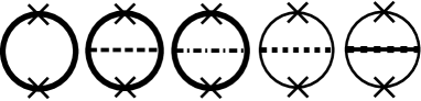
Figure 4: Diagrams relevant to the calculation of the pion mass and its decay constant in the OPT expansion up to ${\cal O}(\delta)$. The thick continuous line represents vacuum fermionic propagators for quarks with all colors, which are evaluated when $\Delta=\Delta_{c}=0$; the thin line represents vacuum fermionic propagators for only quarks with colors 1 and 2; the dashed line represents the chiral bosonic scalar $\zeta$ field propagator; the dash-dotted one represents the pion $\vec{\pi}$-fields propagator; the dotted one is related to the $\phi_{R}$ field; and the continuous-dotted line is associated with the $\phi_{I}$ field. In addition, the vertex pairs represented by an “X” in each diagram can be $\gamma^{5}\tau_{i,j}$ (in the case of the pion mass equation) or $\gamma^{5}\gamma_{\mu,\nu}\tau_{i,j}$ (in the case of the decay constant equation). All quantities are calculated when $\delta=1$.

The free fermion propagators shown in Fig. 4 and related to the quarks $q_{1}$ and $q_{2}$ (red and green in color space) and to $q_{3}$ are given, respectively, by

$$iG_{\Psi}^{vac}(p) = iG^{vac}(p)1_{NG},$$ (58)

and

$$iG_{q_{3}}^{vac}(p) = iG^{vac}(p),$$ (59)

where

$$G^{vac}(p)=\frac{\not{p}+\mathcal{M}}{p^{2}-\mathcal{M}^{2}+i\epsilon},$$ (60)

and $\Psi$ represents the quarks $q_{1}$ and $q_{2}$ in the Nambu-Gor’kov space gorkov ; Nambu:1960tm , with $1_{NG}$ being the identity matrix in this space.

The one-loop diagram shown in Fig. 4, when using the vertex $\tau_{i}\gamma^{5}$ and the Feynman rules obtained from Eq. (12), can be written explicitly in the form

$$i\Pi_{\pi}^{(1)}(q^{2})\delta_{ij} = -\int\frac{d^{4}p}{(2\pi)^{4}}\mathrm{Tr}_{c,f,D}\left[iG^{vac}(p)(\tau_{i}\gamma^{5})\right.$$ (61)

$$\times \left.iG^{vac}(p+q)(\tau_{j}\gamma^{5})\right],$$

where $q$ denotes here the external momentum and $\delta=1$ is considered in this and in all subsequent terms evaluated in the OPT expansion. After we perform the traces in flavor and color spaces, we find

$$\Pi_{\pi}^{(1)}(q^{2}) = 2iN_{c}N_{f}\left[2I_{G}(\mathcal{M})-q^{2}I(q^{2})\right],$$ (62)

where

$$I_{G}(\mathcal{M})=\int\frac{d^{4}p}{(2\pi)^{4}}\frac{1}{p^{2}-\mathcal{M}^{2}+i\epsilon}=-\frac{i}{2}I_{2},$$ (63)

and

$$\!\!\!\!\!\!\!\!\!\!\!\!I(q^{2})\!=\!\!\int\!\frac{d^{4}p}{(2\pi)^{4}}\frac{1}{(p^{2}\!-\!\mathcal{M}^{2}\!+\!i\epsilon)[(p\!+\!q)^{2}\!-\!\mathcal{M}^{2}+i\epsilon]}.$$ (64)

The self-energy terms generated by the two-loop diagrams, given by the second and third diagrams shown in Fig. 4 and related to the scalar $\zeta$ and pion $\vec{\pi}$ chiral fields can be written, respectively, as

$$-i\Pi_{\pi\ ij}^{(2),\zeta}(q^{2}) = -i2G_{s}\int_{p_{1},p_{2}}\mathrm{Tr}_{c,f,D}\left[(-i)iG^{vac}(p_{1})(\tau_{i}\gamma^{5})\right.$$ (65)

$$\times \left.iG^{vac}(p_{1}+q)(-i)iG^{vac}(p_{2}+q)\right.$$

$$\times \left.(\tau_{j}\gamma^{5})iG^{vac}(p_{2})\right],$$

and

$$-i\Pi_{\pi\ ij}^{(2),\vec{\pi}}(q^{2}) = -i2G_{s}\int_{p_{1},p_{2}}\mathrm{Tr}_{c,f,D}\left[(\tau_{k}\gamma^{5})iG^{vac}(p_{1})\right.$$ (66)

$$\times \left.(\tau_{i}\gamma^{5})iG^{vac}(p_{1}+q)(\tau_{k}\gamma^{5})iG^{vac}(p_{2}+q)\right.$$

$$\times \left.(\tau_{j}\gamma^{5})iG^{vac}(p_{2})\right],$$

where

$$\int_{p_{1},p_{2}}\equiv\int\frac{d^{4}p_{1}}{(2\pi)^{4}}\frac{d^{4}p_{2}}{(2\pi)^{4}}.$$ (67)

Evaluating again the traces in the above expressions, we obtain

$$\Pi_{\pi}^{(2),\zeta}(q^{2}) = -8G_{s}N_{c}N_{f}\left\{\frac{}{}I_{G}^{2}(\mathcal{M})-q^{2}\left[\vphantom{\frac{q^{2}}{4}}I_{G}(\mathcal{M})I(q^{2})\right.\right.$$ (68)

$$- \left.\left.\mathcal{M}^{2}I^{2}(q^{2})-\frac{q^{2}}{4}I^{2}(q^{2})\right]\right\},$$

and

$$\Pi_{\pi}^{(2),\vec{\pi}}(q^{2}) = -8(n_{\pi}-2)G_{s}N_{c}N_{f}\left\{\frac{}{}I_{G}^{2}(\mathcal{M})\right.$$

$$- q^{2}\left.\left[I_{G}(\mathcal{M})I(q^{2})+\mathcal{M}^{2}I^{2}(q^{2})-\frac{q^{2}}{4}I^{2}(q^{2})\right]\right\}\ ,$$

where

$$\Pi_{\pi\ ij}^{(2),\zeta}(q^{2}) = \Pi_{\pi}^{(2),\zeta}(q^{2})\delta_{ij},$$

$$\Pi_{\pi\ ij}^{(2),\vec{\pi}}(q^{2}) = \Pi_{\pi}^{(2),\vec{\pi}}(q^{2})\delta_{ij}.$$ (70)

The contributions of the last two diagrams shown in Fig. 4 are related to the real and imaginary components of the diquark scalar field, $\phi_{R}$ and $\phi_{I}$, respectively. In this case, only the vacuum propagator relative to the Nambu-Gor’kov spinor $\Psi$, given by Eq. (58), needs to be taken into account. Explicitly, we have that

$$-i\Pi_{\pi\ ij}^{(2),\phi_{R}}(q^{2}) = \frac{1}{2}(-i2G_{d})\int_{p_{1},p_{2}}\mathrm{Tr}_{all}\left[i^{2}\gamma^{5}\tau_{2}t_{2}\begin{pmatrix}0&1\\ 1&0\end{pmatrix}iG_{\Psi}^{vac}(p_{1})\gamma^{5}\begin{pmatrix}\tau_{i}&0\\ 0&\tau_{i}^{T}\end{pmatrix}iG_{\Psi}^{vac}(p_{1}+q)\right.$$ (71)

$$\times \left.i^{2}\gamma^{5}\tau_{2}t_{2}\begin{pmatrix}0&1\\ 1&0\end{pmatrix}iG_{\Psi}^{vac}(p_{2}+q)\gamma^{5}\begin{pmatrix}\tau_{j}&0\\ 0&\tau_{j}^{T}\end{pmatrix}iG_{\Psi}^{vac}(p_{2})\right],$$

and

$$-i\Pi_{\pi\ ij}^{(2),\phi_{I}}(q^{2}) = \frac{1}{2}(-i2G_{d})\int_{p_{1},p_{2}}\mathrm{Tr}_{all}\left[(-i^{2}\gamma^{5}\tau_{2}t_{2})\begin{pmatrix}0&-i\\ i&0\end{pmatrix}iG_{\Psi}^{vac}(p_{1})\gamma^{5}\begin{pmatrix}\tau_{i}&0\\ 0&\tau_{i}^{T}\end{pmatrix}iG_{\Psi}^{vac}(p_{1}+q)\right.$$ (72)

$$\times \left.(-i^{2}\gamma^{5}\tau_{2}t_{2})\begin{pmatrix}0&-i\\ i&0\end{pmatrix}iG_{\Psi}^{vac}(p_{2}+q)\gamma^{5}\begin{pmatrix}\tau_{j}&0\\ 0&\tau_{j}^{T}\end{pmatrix}iG_{\Psi}^{vac}(p_{2})\right],$$

where $\mathrm{Tr}_{all}$ also incorporates the trace in the Nambu-Gor’kov space.

It is easy to show that $\Pi_{\pi\ ij}^{(2),\phi_{R}}(q^{2})=\Pi_{\pi\ ij}^{(2),\phi_{I}}(q^{2})$. Therefore, we only have to calculate Eq. (71) or, equivalently, Eq. (72). After the calculation of the traces, we obtain the joint contribution of the two diagrams:

$$\Pi_{\pi}^{(2),\phi}(q^{2}) \equiv \Pi_{\pi}^{(2),\phi_{R}}(q^{2})+\Pi_{\pi}^{(2),\phi_{I}}(q^{2})$$

$$= 2\Pi_{\pi}^{(2),\phi_{R}}(q^{2})$$

$$= -16G_{d}(N_{c}-1)N_{f}\left\{\frac{}{}I_{G}^{2}(\mathcal{M})\right.$$

$$- \left.q^{2}\left[I_{G}(\mathcal{M})I(q^{2})+\mathcal{M}^{2}I^{2}(q^{2})-\frac{q^{2}}{4}I^{2}(q^{2})\right]\right\}.$$

The pion mass $m_{\pi}$ is the pole of its propagator. This means that Eq. (57) should be null when we make $q^{2}\rightarrow m_{\pi}^{2}$. Since $\Pi_{\pi}(q^{2})$ is the sum of Eqs. (62), (LABEL:Pipion), (68), and (LABEL:Pidiquark), we can write

$$0 = 1-2G_{s}\Pi_{\pi}(m_{\pi}^{2})$$ (74)

$$= 1-4iG_{s}N_{c}N_{f}\left[2I_{G}(\mathcal{M})-m_{\pi}^{2}I(m_{\pi}^{2})\right]$$

$$+ 4N_{c}N_{f}G^{2}_{s}\left\{f(G_{d})\left[2I_{G}(\mathcal{M})-m_{\pi}^{2}I(m_{\pi}^{2})\right]^{2}\right.$$

$$- \left.4\left[f(G_{d})-2\right]m_{\pi}^{2}\mathcal{M}^{2}I^{2}(m_{\pi}^{2})\right\}\;,$$

where $f(G_{d})$ was already defined in Eq. (54), and the integral $I(m_{\pi}^{2})$ is given by

$$I(m_{\pi}^{2}) = \frac{i}{8\pi^{2}}\left[\mathrm{ln}\left(\frac{\Lambda+\sqrt{\Lambda^{2}+\mathcal{M}^{2}}}{\mathcal{M}}\right)-\sqrt{4\frac{\mathcal{M}^{2}}{m_{\pi}^{2}}-1}\right.$$

$$\times \left.\mathrm{tan}^{-1}\left(\frac{\Lambda}{\sqrt{\Lambda^{2}+\mathcal{M}^{2}}\sqrt{4\mathcal{M}^{2}/m_{\pi}^{2}-1}}\right)\right].$$

Now, iterating once the PMS equation (53) and substituting in the gap equation (51), we get the relation

$$\frac{m}{M_{q}^{OPT}} = 1-8iG_{s}N_{c}N_{f}I_{G}(\mathcal{M})$$ (76)

$$+ 16f(G_{d})G_{s}^{2}N_{c}N_{f}I_{G}^{2}(\mathcal{M}),$$

which, when inserted into Eq. (74), gives us the result

$$\frac{m}{M_{q}^{OPT}} = 4G_{s}N_{c}N_{f}m_{\pi}^{2}\left\{\vphantom{\left(\mathcal{M}^{2}-\frac{m_{\pi}^{2}}{4}\right)}-iI(m_{\pi}^{2})+4f(G_{d})G_{s}\right.$$ (77)

$$\times \left.\left[I_{G}(\mathcal{M})I(m_{\pi}^{2})+\left(\mathcal{M}^{2}-\frac{m_{\pi}^{2}}{4}\right)I^{2}(m_{\pi}^{2})\right]\right.$$

$$- \left.8G_{s}\mathcal{M}^{2}I^{2}(m_{\pi}^{2})\vphantom{\left(\mathcal{M}^{2}-\frac{m_{\pi}^{2}}{4}\right)}\right\}.$$

We can clearly see that Eq. (77) satisfies the Goldstone theorem. When we take $m=0$ (the chiral case) in Eq. (77), we automatically obtain $m_{\pi}=0$, consistent with the Goldstone theorem.

V.2 The pion decay constant equation

Let us now evaluate the pion decay constant in the OPT expansion to order $\delta$. The pion decay constant can be expressed as RUDOPT

$$\langle 0|TA_{\mu}^{i}(q)A_{\nu}^{j}(0)|0\rangle=ig_{\mu\nu}\delta^{ij}f_{\pi}^{2}+\mathcal{O}(q_{\mu}q_{\nu}),$$ (78)

where $A_{\mu}^{i}\equiv\bar{\psi}\gamma_{\mu}\gamma_{5}(\tau^{i}/2)\psi$. In practice, we can take advantage of all the diagrams of Fig. 4 again, but we replace the vertex $\gamma^{5}\tau_{i,j}$ with $\gamma^{5}\gamma_{\mu}\tau_{i,j}/2$ to compute $f_{\pi}^{2}$. Since the calculations are analogous, yet more laborious than those made previously to obtain the expression containing the pion mass, we show some the details in the Appendix. From the results given there, we extract that the contribution from each loop term contributing to $f_{\pi}$ can be expressed in the form

$$f_{\pi,1}^{2} = -2iN_{c}N_{f}\mathcal{M}^{2}I(0),$$ (79)

$$f_{\pi,\zeta}^{2} = 4G_{s}N_{c}N_{f}\mathcal{M}^{4}I^{2}(0),$$ (80)

$$f_{\pi,\vec{\pi}}^{2} = 4G_{s}N_{c}N_{f}(n_{\pi}-2)\mathcal{M}^{4}I^{2}(0),$$ (81)

$$f_{\pi,\phi}^{2} = 8G_{d}(N_{c}-1)N_{f}\mathcal{M}^{4}I^{2}(0),$$ (82)

with the integral $I(0)$ obtained from the limit $q^{2}\rightarrow 0$ applied to Eq. (64), which gives

$$I(0) = \frac{i}{8\pi^{2}}\left[\mathrm{sinh}^{-1}\left(\frac{\Lambda}{\mathcal{M}}\right)-\frac{\Lambda}{\sqrt{\Lambda^{2}+\mathcal{M}^{2}}}\right].$$ (83)

The final expression for $f_{\pi}^{2}$ is obtained by adding Eqs. (79), (80), (81), and (82), which finally gives

$$f_{\pi}^{2} = -2iN_{c}N_{f}\mathcal{M}^{2}I(0)+4N_{c}N_{f}G_{s}f(G_{d})\mathcal{M}^{4}I^{2}(0).$$

V.3 The complete fitting expressions in the OPT expansion to ${\cal O}(\delta)$

The complete set of consistent equations that need to be solved in order to provide the values of the parameters, once the numerical data for $m_{\pi}$, $f_{\pi}$, and $\langle\bar{q}q\rangle$ are provided, is then

$$M_{q}^{OPT}=m+4G_{s}N_{c}N_{f}\mathcal{M}I_{2},$$ (85)

$$\mathcal{M}=M_{q}^{OPT}+f(G_{d})G_{s}\mathcal{M}I_{2},$$ (86)

$$\langle\bar{\psi}\psi\rangle=-\frac{M_{q}^{OPT}-m}{4G_{s}},$$ (87)

$$f_{\pi}^{2}=-2iN_{c}N_{f}\mathcal{M}^{2}I(0)+4f(G_{d})N_{c}N_{f}G_{s}\mathcal{M}^{4}I^{2}(0),$$

and

$$\frac{m}{M_{q}^{OPT}} = 4G_{s}N_{c}N_{f}m_{\pi}^{2}\left\{\vphantom{\left(\mathcal{M}^{2}-\frac{m_{\pi}^{2}}{4}\right)}-iI(m_{\pi}^{2})+4f(G_{d})G_{s}\right.$$ (89)

$$\times \left.\left[I_{G}(\mathcal{M})I(m_{\pi}^{2})+\left(\mathcal{M}^{2}-\frac{m_{\pi}^{2}}{4}\right)I^{2}(m_{\pi}^{2})\right]\right.$$

$$- \left.8G_{s}\mathcal{M}^{2}I^{2}(m_{\pi}^{2})\vphantom{\left(\mathcal{M}^{2}-\frac{m_{\pi}^{2}}{4}\right)}\right\}\ .$$

Table 1: Parameter values used in the OPT scheme and in the LN approximation (last line). The inputs used are $m_{\pi}=134\ \mathrm{MeV}$, $f_{\pi}=93\ \mathrm{MeV}$, and $-\langle\bar{\psi}\psi\rangle^{1/3}=250\ \mathrm{MeV}$.

$G_{d}/G_{s}$	$M_{q}\ (\mathrm{MeV})$	$m\ (\mathrm{MeV})$	$G_{s}\ (\mathrm{GeV}^{-2})$	$\Lambda\ (\mathrm{MeV})$
$1.3$	$293.445$	$4.777$	$4.619$	$640.112$
$1.4$	$292.973$	$4.760$	$4.611$	$639.597$
$1.5$	$292.520$	$4.744$	$4.604$	$639.077$
1.53	292.389	4.739	4.602	638.920
1.54	292.345	4.737	4.602	638.867
1.55	292.302	4.735	4.601	638.815
LN	$313.519$	$4.987$	$4.937$	$653.331$

From the input values, we obtain numerically, sets of parameters for some values of $G_{d}/G_{s}$, as shown in Table 1. Note that, as compared to the LN approximation, the corrections due to OPT cause a slight drop in all parameters of the table, and this fall is intensified with increasing coupling between quarks (represented by $G_{d}$). The LN approximation, which can be obtained when we neglect the OPT two-loop contributions in the equations that compose the system, does not provide parameters that depend on $G_{d}$, as already explained, since diquark fluctuations would contribute with subleading $1/N_{c}$ correction terms, but these terms do contribute in the OPT case. The values corresponding to the ratios $G_{s}/G_{d}=1.53,\,1.54$, and $1.55$ and shown in the Tab. 1 will be used when imposing the color neutrality condition, while the other values will be used in the absence of color neutrality and in the comparison of our OPT results with those obtained in the LN approximation.

VI Numerical results using the OPT for the cold and dense system

Before presenting our results, it is useful to first recall a few properties regarding the BEC-BCS crossover and the requirement for color neutrality.

VI.1 The BEC-BCS crossover

If we start from the dispersion relation e.g., the one from the mean field LN approximation, from Eq. (15) and set $\delta=0$, $\mu^{\prime}=\mu$ (red and green quarks), $\alpha_{s}\to\Delta$, and $\eta\to\sigma$, we have, for example, $E_{\Delta,\vec{p}}^{-}(\mu)=\sqrt{\left[\sqrt{p^{2}+M_{q}^{2}}-\mu\right]^{2}+\Delta^{2}}$. For small chemical potential $\mu\leq M_{q}$, the minimum of the dispersion is located at $|\vec{p}|=0$, with particle gap energy $\sqrt{M_{q}^{2}+\Delta^{2}}$, which would correspond to the fermionic (quark) spectrum in the BEC state. At values of chemical potential such that $\mu>M_{q}$, the minimum of the dispersion is shifted to $|\vec{p}|\neq 0$, and the particle gap is $\Delta$. This corresponds to the fermionic spectrum in the BCS state. It is then useful to define an effective chemical potential $\mu_{N}\equiv\mu-M_{q}$, which will serve as an indicator of the BEC-BCS crossover SUNHE .

VI.2 Color neutrality condition

In the model given by Eq. (1) for $N_{c}=3$, in the choice that allows only red and green color quarks to form diquarks and that leaves out the blue ones, for example, it follows that when equal chemical potentials are introduced for the three colors $\mu_{r}=\mu_{g}=\mu_{b}\equiv\mu_{B}/3$, where $\mu_{B}$ represents the baryon chemical potential the phase characterized by the absence of the diquark condensate, $\Delta_{c}=0$, keeps the color symmetry $SU(3)$, while the phase at which the condensate is nonzero, $\Delta_{c}\neq 0$, breaks the $SU(3)$ color symmetry down to $SU(2)$. However, in the latter case, the number densities of the quarks that form the diquarks, $n_{r}$ and $n_{g}$, are identical and are larger than the density of the blue-colored quarks, $n_{b}$ BubaShov ; Diet ; EBERTKLIM2 ; SUNHE . This means that in this phase, the system as a whole does not have the property of color neutrality, which is physically verified. In fact, such a situation also occurs in QCD when we consider the two-flavor superconducting color phase, but it is possible to generate the eighth gluon field, which guarantees the color neutrality automatically EBERTKLIM2 in theory. Effectively, it generates a chemical potential $\mu_{8}$. Since in the NJL model we do not have gluon degrees of freedom, what is done to ensure color neutrality is to add by hand a chemical potential term $\mu_{8}$ in the Lagrangian density of the theory – $\mu_{8}\bar{\psi}\gamma^{0}T_{8}\psi$, with $T_{8}=\sqrt{3}\lambda_{8}$ – and impose that $\langle Q_{8}\rangle=0$, which is equivalent to demanding the condition

$$n_{8}=-\frac{\partial\Omega}{\partial\mu_{8}}=0,$$ (90)

where $\Omega$ is the thermodynamic potential in the desired approximation. Furthermore, in practice, the chemical potential $\mu_{8}$ enters in the final expressions obtained. Until then, we can simply make the changes SUNHE $\mu_{g}=\mu_{r}=\mu\rightarrow\mu_{B}/3+\mu_{8}/3$ and $\mu_{b}\rightarrow\mu_{B}/3-2\mu_{8}/3$. This will be the procedure we will also follow here when demanding color neutrality.

Note that besides the imposition of color neutrality, electric charge neutrality in principle should also be considered. Including electric charge neutrality introduces an extra chemical potential, $\mu_{Q}$, which is proportional to the electric charges for the $u$ and $d$ quarks and introduces an explicit difference in chemical potentials for these quarks. This difference in chemical potentials can lead to some important effects, such as a gapless color superconducting phase Huang:2002zd ; Shovkovy:2003uu . Since in this work we are primarily interested in the comparison of the LN results for the BEC-BCS crossover with the OPT ones, we will here neglect for simplicity the condition of electric charge neutrality, as was the case also in the previous works EBERTKLIM2 ; SUNHE . But we should keep in mind that for any realistic application, such as in the determination of the equation of state relevant for the physics of compact stellar objects, both of the conditions of color – electric charge neutrality and $\beta$-equilibrium – should be imposed.

VI.3 Numerical results: Absence of color neutrality

We now turn to the numerical results obtained with the OPT method and the comparison of these results with those obtained using the LN approximation. For simplicity and making easier the comparison between the OPT and LN results, we will first analyze the case of the absence of color neutrality (e.g., we consider $\mu_{8}=0$ initially), and we can assume simply, as previously stated, that $\mu_{r}=\mu_{b}=\mu_{g}\equiv\mu_{B}/3$.

From the OPT thermodynamic potential at zero temperature, $V_{\rm eff}^{OPT}(\sigma_{c},\Delta_{c})$, given by the sum of Eqs. (31), (32), and (33), together with the corresponding gap equations for the chiral and diquark condensates,

$$\left.\frac{\partial V_{\rm eff}}{\partial\sigma}\right|_{\sigma=\sigma_{c}}=0,\qquad\left.\frac{\partial V_{\rm eff}}{\partial\Delta}\right|_{\Delta=\Delta_{c}}=0,$$ (91)

and the PMS conditions, Eqs. (22) and (23), applied to the OPT mass parameters $\eta$ and $\alpha$, we can find numerically the behavior for the chiral condensate $\sigma$ (and consequently, that for the effective quark mass $M_{q}$) and diquark condensate $\Delta$, as well as all the relevant thermodynamic properties of the system, as a function of the chemical potential. (For convenience we drop the subscript $c$ in $\sigma$ and $\Delta$ from now on.) In the absence of color neutrality, we can write the effective chemical potential characterizing the BEC-BCS crossover simply as $\mu_{N}=\mu_{B}/3-M_{q}$. As in conventional in the literature, we will present the results as a function of the baryon chemical potential $\mu_{B}$.

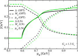
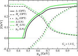
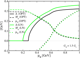
Figure 5: Diquark condensate $\Delta$, effective mass $M_{q}$, and effective chemical potential $\mu_{N}$ as a function of the baryon chemical potential $\mu_{B}$ for different values of the ratio $G_{d}/G_{s}$ in the LN approximation and OPT comparatively.

We start by showing in Fig. 5 the behavior of the effective quark mass $M_{q}$ and $\Delta$ with the increase of the baryon chemical potential $\mu_{B}$ for $G_{d}/G_{s}=1.3,\,1.4$ and $1.5$, which were the same values considered in Ref. SUNHE , which studied the BEC-BCS crossover in the LN approximation. The $\mu_{N}$ result for each method is also indicated in the plots, such as to facilitate visualization of the BEC region, which corresponds to the values of $\mu_{B}$ for which $\mu_{N}<0$, when $\Delta\neq 0$, going to $\mu_{N}>0$, corresponding to the BCS region. The results in Fig. 5 indicate that OPT disfavors the BEC region and that this region seems to decrease more significantly with the decrease of the ratio $G_{d}/G_{s}$. In addition, we observe that the OPT also disfavors the region in which $\Delta\neq 0$ for $1.3\lesssim G_{d}/G_{s}\lesssim 1.5$, increasing the value of critical chemical potential(s) $\mu_{B,c}$ (OPT) relative to those of the LN approximation. From the qualitative point of view, the variation of $\Delta$ and $M_{q}^{OPT}$ with the variation of $\mu_{B}$ remain similar to the ones observed in the LN case, while maintaining the phase transition as being second order when color neutrality is not required, as shown in Fig. 6.

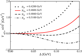
Figure 6: The effective potential in the OPT at zero temperature with the vacuum energy subtracted, $V_{\rm eff}\equiv V_{\rm eff}(\sigma,\Delta,\bar{\eta},\bar{\alpha},\mu_{B})-V_{\rm eff}(\sigma_{vac},\Delta=0,\bar{\eta}_{vac},\bar{\alpha},\mu_{B}=0)$, as a function of $\Delta$ for different values of baryon chemical potential $\mu_{B}$ around the critical value $\mu_{B,c}=0.4686$ GeV , for the ratio $G_{d}/G_{s}=1.4$. The evolution of the global mininum of potential when changing $\mu_{B}$ suggests a second-order phase transition in the order parameter $\Delta$, as occurs in the LN case.

By looking again at Fig. 5, we note that the value of the condensate $\Delta$ given by the OPT is always smaller than the one given by the LN approximation, and this difference becomes larger with the increase of $G_{d}/G_{s}$. In addition, we observe that $M_{q}^{OPT}$ increasingly approaches $M_{q}^{LN}$ for increasing values of $G_{d}/G_{s}$ and $\mu_{B}$. The difference between these quantities – for example, for the case $G_{d}/G_{s}=1.5$ – is visually insignificant from the critical chemical potential $\mu_{B,c}$ (OPT) of the phase transition in OPT. Something similar occurs with the chemical potential for which occurs the BEC-BCS crossover, obtained by the condition $\mu_{N}=0$, $\mu_{B,c}^{\rm BEC-BCS}$. In the OPT, the crossover requires a value of $\mu_{B,c}^{\rm BEC-BCS}$ (OPT) that is lower than that of in the LN approximation case, and this difference tends to decrease appreciably with the increase of $G_{d}/G_{s}$.

These results concerning the BEC-BCS crossover and the differences between the LN and OPT critical values are summarized in the Table 2, where, for completeness, we also show the value for the pseudocritical chemical potential, $\mu_{B,pc}^{\rm ch}$, for the chiral symmetry crossover (defined by the position of the inflection point in $M_{q}$).

Table 2: Values of critical chemical potentials for the LN and OPT, in both cases in the absence of color neutrality.

No color neutrality case
	$G_{d}/G_{s}$	$\mu_{B,c}$ (GeV)	$\mu_{B,c}^{\rm BEC-BCS}$ (GeV)	$\mu_{B,pc}^{\rm ch}$ (GeV)
	1.3	0.6003	0.7051	0.7398
LN	1.4	0.4513	0.6334	0.6785
	1.5	0.2010	0.5557	0.6104
	1.3	0.5972	0.6820	0.7306
OPT	1.4	0.4686	0.6155	0.6742
	1.5	0.2787	0.5454	0.6134

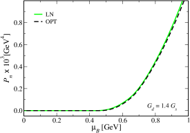
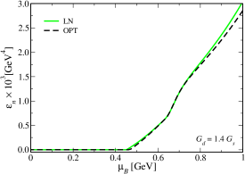
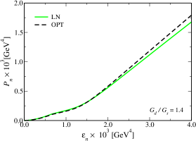
Figure 7: The pressure (top plot), the energy density as a function of $\mu_{B}$ (middle plot) and the equation of state (bottom plot), both for the ratio $G_{d}/G_{s}=1.4$.

To also exemplify some of the differences between OPT and LN for other thermodynamic quantities, in Fig. 7 we show the vacuum subtracted pressure and energy densities, $P_{n}(\sigma,\Delta)$ and $\varepsilon_{n}(\sigma,\Delta)$, respectively, in addition to the equation of state $P_{n}(\varepsilon_{n})$, where $P_{n}=P-P_{vac}$ and $\varepsilon_{n}=\varepsilon-\varepsilon_{vac}$, with (at $T=0$)

$$P(\sigma,\Delta) = -V_{\rm eff}(\sigma,\Delta),$$ (92)

$$\varepsilon(\sigma,\Delta) = -P(\sigma,\Delta)+\mu_{B}n_{B},$$ (93)

where $n_{B}$ is the baryon number density, given by

$$n_{B}=-\frac{\partial}{\partial\mu_{B}}V_{\rm eff}(\sigma,\Delta).$$ (94)

We have restricted Fig. 7 to show only the case $G_{d}/G_{s}=1.4$ as an example. Visually, there is no significant differences between such cases in the region of interest. But in the region of intermediate baryon chemical potentials, the OPT slightly decreases its values compared to the LN approximation for the value of $G_{d}/G_{s}$ used herein.

VI.4 The OPT results in the case of color neutrality

Let us now consider the case of imposing the color neutrality condition. As already discussed above, in this case we set $\mu=\mu_{B}/3+\mu_{8}/3$, $\mu_{b}=\mu_{B}/3-2\mu_{8}/3$, and the condition of color neutrality, given by Eq. (90), must be satisfied in the region where $\Delta\neq 0$, that represents the physical case.

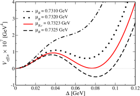
Figure 8: The vacuum subtracted effective potential in the OPT at zero temperature as a function of $\Delta$, for different values of the baryon chemical potential $\mu_{B}$ around the critical value $\mu_{B,c}=0.7323$ GeV and for the ratio $G_{d}/G_{s}=1.3$. The behavior of the global minimum of potential with the variation of $\mu_{B}$ and the coexistence between the two minima suggests a first-order phase transition in the order parameter $\Delta$.

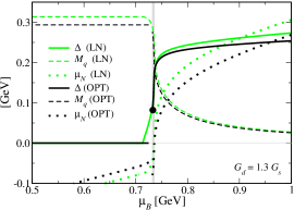
Figure 9: The diquark condensate $\Delta$, the effective quark mass $M_{q}$, and the effective chemical potential $\mu_{N}$ as a function of the baryon chemical potential $\mu_{B}$ for $G_{d}/G_{s}=1.3$, in the LN approximation and OPT comparatively. Color neutrality is considered. The thin vertical line indicates the position of the first-order transition (discontinuity) in $\Delta$.

The main effect coming from the corrections due to the OPT in relation to the case of LN, for the values of $G_{d}/G_{s}$ previously considered, is that there is a discontinuity in $\Delta(\mu_{B})$ at the critical baryon chemical potential $\mu_{B,c}$ (OPT), indicating a first-order phase transition. The emergence of a first-order transition in this case can be confirmed and illustrated in Figs. 8 and 9, where in both cases we have considered the case $G_{d}/G_{s}=1.3$ as an example. In this case, when the baryon chemical potential increases, the potential presents a new (local) minimum around $\mu_{B}\simeq 0.7113$ GeV, and at the critical baryon chemical potential $\mu_{B,c}\simeq 0.73226$ GeV, this minimum is aligned to the one at $\Delta=0$. If we keep increasing the chemical potential, the minimum at origin becomes local, and after that, a maximum point, around $\mu_{B}\simeq 0.7365$ GeV emerges. This interval, 0.7113 GeV $\lesssim\mu_{B}\lesssim$ 0.7365 GeV, corresponds to a metastable region, represented by the thin vertical gray region in Fig. 9. In the LN case, the BEC region, when contrasted with the case shown in Fig. 5 obtained when neglecting color neutrality, also shrinks, but it does not disappear completely, consistent with the observations made in Ref. SUNHE .

We should remark that in the LN approximation, the transition eventually also turns first order, but for values of the ratio $G_{d}/G_{s}\lesssim 1.05$, as observed in Refs. SUNHE ; Kitazawa:2007zs . By increasing the ratio $G_{d}/G_{s}$, we can again recover a second-order transition for the phase with a diquark condensate and a BEC-BCS crossover. For the OPT case, we find that the minimum value required for a second-order phase transition shifts from $G_{d}/G_{s}\approx 1.05$ in the LN case to a value $G_{d}/G_{s}\approx 1.525$, which is itself very close to the maximum value allowed for the ratio $G_{d}/G_{s}$ before the mass of the diquark vanishes, precluding the instability of the vacuum. In the OPT, for the parameters considered, this happens for values $G_{d}/G_{s}>1.55$.

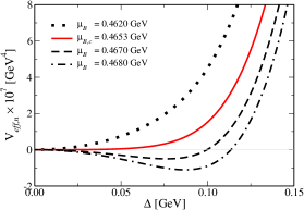
Figure 10: The vacuum subtracted effective potential in the OPT at zero temperature as a function of $\Delta$ for different values of baryon chemical potential $\mu_{B}$ around the critical value $\mu_{B,c}=0.4653$ GeV, for $G_{d}/G_{s}=1.53$. The behavior of the global minimum of potential with the variation of $\mu_{B}$ suggests a second-order phase transition in the order parameter $\Delta$. Color neutrality is considered.

In Fig. 10, we show the effective potential in the OPT for the case of $G_{d}/G_{s}=1.53$, confirming the resurgence of the second-order phase transition for diquark condensation.

Next, we will restrict our attention to the cases where a second-order phase transition for diquark condensation is possible in the OPT, which will in particular correspond to the cases where the ratio of $G_{d}/G_{s}$ will assume the values $G_{d}/G_{s}=1.53,\,1.54$, and $1.55$.

In Fig. 11, we show the results for $\Delta,M_{q}$, and $\mu_{N}$ for the values $G_{d}/G_{s}=1.53,\,1.54$, and $1.55$. It is possible to see that, similarly to the LN case with results shown in Fig. 5, as we increase the ratio $G_{d}/G_{s}$, the OPT favors the BEC phase. The critical baryon chemical potential $\mu_{B,c}$ and the crossover value $\mu_{B,c}^{\rm BEC-BCS}$ both decrease as the ratio $G_{d}/G_{s}$ increases. But $\mu_{B,c}$ is more affected by the value of $G_{d}/G_{s}$. In the LN case, however, both $\mu_{B,c}$ and $\mu_{B,c}^{\rm BEC-BCS}$ suffer similar influence due to a variation of of $G_{d}/G_{s}$. Both of these results can be seen in Fig. 12.

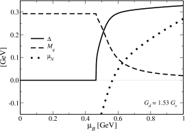
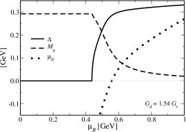
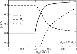
Figure 11: Diquark condensate $\Delta$, effective mass $M_{q}$, and effective chemical potential $\mu_{N}$ as a function of baryon chemical potential $\mu_{B}$ for different values of $G_{d}/G_{s}$ in the OPT case. Color neutrality is considered.

In Fig. 12, we illustrate the evolution of the critical points $\mu_{B,c}$, $\mu_{B,c}^{\rm BEC-BCS}$, while in Fig. 13 we give the width of the BEC region, defined by $(\mu_{B,c}^{\rm BEC-BCS}-\mu_{B,c})$ as a function of $G_{d}/G_{s}$, for both the LN and OPT cases.

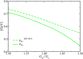
(a) LN case.

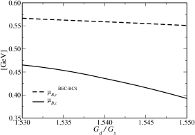
(b) OPT case.

Figure 12: The critical chemical potentials associated with the BEC phase transition $\mu_{B,c}$, as a function of $G_{d}/G_{s}$, for the LN and OPT cases, in their correspondent validity range. Color neutrality is considered in both cases.

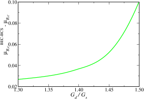
(a) LN case.

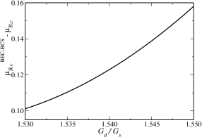
(b) OPT case.

Figure 13: The width of the BEC region, defined by $(\mu_{B,c}^{\rm BEC-BCS}-\mu_{B,c})$, as a function of $G_{d}/G_{s}$, for the LN and OPT cases, in their correspondent validity range. Color neutrality is considered in both cases.

In Table 3 we summarize the values for the critical chemical potentials obtained when considering the color neutrality condition in the LN and OPT cases. For completeness, we also give the values for the pseudocritical chemical potential for chiral condensation, $\mu_{B,pc}^{\rm ch}$. Note that the critical baryon chemical potential for the BEC transition always tends to decrease as we increase the ratio $G_{d}/G_{s}$, which is true in both the LN and OPT cases. Note also that the results for the critical baryon chemical potentials always remain below that of the value of the onset of baryonic matter (e.g., when comparing with the nucleon mass), which prompts the question of the reliability of these results when applied to real QCD. In fact, the same trend we see here is also seen in all previous studies for the BEC-BCS crossover study in the NJL model (see, however, Ref. He:2010nb ). As far as this issue is concerned, when we compare the LN and OPT results, we see that while the LN gives a much larger range of values for $G_{d}/G_{s}$ allowing for the BEC phase, in the OPT case this window shrinks considerably to a very small range of values, $1.525\lesssim G_{d}/G_{s}\lesssim 1.55$. In a sense, by including further contributions from both meson and diquark fluctuations (represented by the two-loop contributions) which are absent in the LN approximation, the OPT clearly disfavors the emergence of a BEC phase. This seems more in accordance, based on these results, with the expectancy that the appearance of a diquark BEC phase at low density must be an artificial effect in the (three-color) NJL model.

Table 3: Values of critical chemical potential, considering color neutrality effects, for LN and OPT.

The color neutrality case
	$G_{d}/G_{s}$	$\mu_{B,c}$ (GeV)	$\mu_{B,c}^{\rm BEC-BCS}$ (GeV)	$\mu_{B,pc}^{\rm ch}$ (GeV)
	1.3	0.7137	0.7370	0.7361
LN	1.4	0.6144	0.6603	0.6459
	1.5	0.4474	0.5767	0.5334
OPT	1.53	0.4653	0.5651	0.5213
	1.54	0.4366	0.5573	0.5119
	1.55	0.3939	0.5496	0.5025

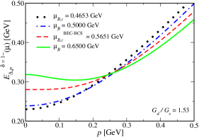
Figure 14: Particle dispersion relation $E_{\Delta,\vec{p}}^{\delta=1-}(\mu)$ in the OPT approximation for $G_{d}/G_{s}=1.53$. Color neutrality is considered.

As already mentioned previously, the BEC-BCS crossover can be characterized by the shape of the dispersion relation for the quark field, which for the OPT case is given by Eq. (15) when setting $\delta=1,\Delta_{1}=\Delta_{2}=\Delta$, $\alpha_{1}=\alpha_{2}=\alpha$, and $\mu^{\prime}=\mu=\mu_{B}/3+\mu_{8}/3$, or $E_{\Delta,\vec{p}}^{\delta=1-}(\mu)=\sqrt{\left[\sqrt{p^{2}+(M_{q}^{OPT})^{2}}-\mu\right]^{2}+\Delta^{2}}$ (the same form as in the LN). In Fig. 14, we illustrate the particle dispersion for the OPT in the color neutrality case for the example of $G_{d}/G_{s}=1.53$. For values of $\mu_{B}\leq\mu_{B,c}^{\rm BEC-BCS}$, the minimum of the dispersion is located at $\vec{p}=0$, and the gap energy is $|\mu_{N}|$ (remembering that $\mu_{N}=\mu-M_{q}^{OPT}$, where $M_{q}^{OPT}=m+\sigma^{OPT}$). The BEC phase corresponds to the region between $\mu_{B,c}$ and $\mu_{B,c}^{\rm BEC-BCS}$. Increasing the chemical potential beyond $\mu_{B,c}^{\rm BEC-BCS}$, this minimum is shifted to $|\vec{p}|\simeq|\mu|$ and the gap becomes equal to $\Delta$, indicating the BCS phase. Note that the diquark condensate $\Delta$, as can be seen from Figs. 5 and 11, tends to remain smaller than the baryon chemical potential. We also find that the critical chemical potential for the BEC transition ($\mu_{c}\equiv\mu_{B,c}/3$) corresponds exactly to half the mass of the diquarks. This can be proofed as follows: The diquark mass can be computed in the OPT scheme similarly to the calculation of the pion mass shown in Sec. V.1, with the appropriate changes – e.g., by replacing the pion vertex $-i\gamma^{5}\tau_{i}$ with that of the diquark boson field with the quarks, $iC\gamma^{5}\tau_{2}t_{2}$ obtained from the bosonized Lagrangian density Eq. (2) – from which we then obtain that the diquark mass is determined by the pole equation obtained in terms of the diquark self-energy $\Pi_{d}(q_{0},\vec{q}\,)$ as

$$0 = 1-2G_{d}\Pi_{d}(q_{0}=m_{d},\vec{q}=0)$$ (95)

$$= 1-2G_{d}\left\{2i(N_{c}-1)N_{f}\left[2I_{G}-m_{d}^{2}I(m_{d}^{2})\right]\right.$$

$$- \left.8(N_{c}-1)N_{f}G_{s}\left[2I_{G}-m_{d}^{2}I(m_{d}^{2})\right]^{2}\right.$$

$$+ \left.16(N_{c}-1)N_{f}G_{s}m_{d}^{2}\mathcal{M}^{2}I^{2}(m_{d}^{2})\right\},$$

where $I_{G}$ is given by Eq. (63) and $I(m_{d})$ is obtained from Eq. (64). Note that Eq. (95) in the LN limit reduces to

$$1 = 4iG_{d}(N_{c}-1)N_{f}\left[2I_{G}-m_{d}^{2}I(m_{d}^{2})\right]$$ (96)

$$= 2G_{d}(N_{c}-1)N_{f}\int\frac{d^{3}p}{(2\pi)^{3}}\left(\frac{1}{E_{\vec{p}}+m_{d}/2}\right.$$

$$+ \left.\frac{1}{E_{\vec{p}}-m_{d}/2}\right),$$

where we have evaluated the integral in $p_{0}$ to obtain the last line in the above equation. Equation (96) agrees with the corresponding LN result of Refs. SUNHE ; ZHUANG . In the OPT case, Eq. (95) is a function of the optimization parameter $\eta$ and must then be solved together with the PMS equation (22). Equation (96) in the LN approximation can be compared with the one determining the diquark condensate $\Delta$ [Eq. (48)], and use of the PMS equations (22) and (23), gives

$$\Delta=2(N_{c}-1)N_{f}G_{d}\bar{\alpha}J_{B}(\mu)\Bigr{|}_{\eta={\bar{\eta}}},$$ (97)

where $J_{B}(\mu)$ is given by Eq. (40). If we set again the LN limit in Eq. (97) and recall that in this case the OPT optimization parameters $\bar{\eta}$ and $\bar{\alpha}$ reduce to $\bar{\eta}=\sigma$ and $\bar{\alpha}=\Delta$, respectively, then Eq. (97) becomes, at the diquark condensation point $\mu_{B}\to\mu_{B,c}$ and where $\Delta\to 0$,

$$1 = 2(N_{c}-1)N_{f}G_{d}\int\frac{d^{3}p}{(2\pi)^{3}}\left(\frac{1}{E_{\vec{p}}+\mu_{B,c}/3}\right.$$ (98)

$$+ \left.\frac{1}{E_{\vec{p}}-\mu_{B,c}/3}\right),$$

and we also recover the LN result for $\mu_{B,c}$ as given in Refs. SUNHE ; ZHUANG . When comparing Eq. (96) with Eq. (98), we see immediately that $\mu_{B,c}/3=m_{d}/2$. Note also that when accounting for color neutrality, the same result follows when we consider that $\mu\to\mu+\mu_{8}/3$ [note that the integral $J_{B}$ in Eq. (97) is only a function of $\mu=\mu_{r}=\mu_{g}$], and the critical baryon chemical potential for diquark condensation shifts accordingly, $\mu_{B,c}/3\to m_{d}/2-\mu_{8}/3$. Since $\mu_{8}$ is in general negative, this corresponds to a increase of the diquark condensation point when color neutrality is considered, which agrees with the results shown, e.g., in Table 3. In the OPT scheme, this comparison between the diquark mass and the value for the condensation point is more involved for two main reasons: First, because now we have to solve Eqs. (95) and (97) subject to the PMS Eqs. (22) and (23) and also the gap equation determining $M_{q}$, which makes the numerical work somewhat more involved. Second and most importantly, there is clearly a mismatch between the order-1 OPT expression for the diquark self-energy leading to Eq. (95) and the corresponding contributions considered at the same order in the OPT for the effective potential. In particular, note that the order-1 OPT contributions to the diquark mass, corresponding to the two-loop diagrams which are similar to the ones seen in Fig. 4 for the pion, turn out to be equivalent to three-loop vacuum diagrams in the effective potential (e.g., when we close the external diquark legs in the self-energy diagrams such as to construct equivalent vacuum terms). These contributions would in fact be order2 in the OPT scheme when seen in the context of the effective potential. Due to this mismatch of terms between the diquark self-energy and the effective potential, we do not expect a perfect agreement for the value of $\mu_{B,c}/3$ obtained from the optimization of the effective potential, with the value of $m_{d}/2$ obtained from Eq. (95). This is a feature of the OPT scheme. Intrinsically, we should optimize a quantity that could produce simultaneous values for both $\mu_{B,c}$ and $m_{d}$. This could be, perhaps, the nonhomogeneous (space- or momentum-dependent) effective action, instead of the effective potential (the zero-momentum homogeneous action). Even so, when we compare results from these different quantities, we obtain, taking as an example the ratio $G_{d}/G_{s}=1.4$ in the absence of charge neutrality, the result $\mu_{B,c}/3=0.1562$ GeV, while the result from Eq. (95) gives $m_{d}/2=0.1596$ GeV, a difference of around $2\%$. Though not a proof, we can take this difference as a rough possible indication of the convergence of the OPT and a signal that when going to the next order, which will now include three-loop terms with similar topology to the ones contributing at the self-energy for the diquark mass, these terms are expected to produce an overall small contribution. This is a generic expectation from the OPT scheme seen in studies of its convergence properties in other models opt6 .

Finally, the observations already made in the absence of color neutrality regarding the thermodynamic quantities, like the pressure, energy density, and equation of state, remain essentially the same for the case with color neutrality. In Fig. 15, we show these quantities for the OPT for the three values of $G_{s}/G_{d}$ considered in the color neutrality example.

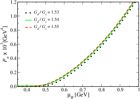
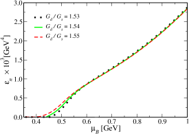
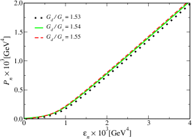
Figure 15: The thermodynamic quantities of the system (normalized pressure $P_{n}$ and normalized energy density $\varepsilon_{n}$) are given for different values of $G_{d}/G_{s}$ as a function of the baryon chemical potential $\mu_{B}$ at zero temperature on OPT approximation, as well as the state equation $P_{n}(\varepsilon_{n})$. Color neutrality is considered.

VII Conclusions

We have studied the BEC-BCS crossover in an extended two-flavor NJL model, with three colors and including the diquark interactions, in the context of the nonperturbative OPT, method and the results obtained were contrasted with those of the usual LN approximation. We derived in detail how the fitting of the parameters changes in the OPT case, deriving the corresponding corrections due to the OPT for the pion mass and decay constant. These quantities are affected by the diquark fluctuations already at first order in the OPT approximation and must be evaluated consistently.

We have studied the cases both of without and with color neutrality and have shown the differences between the two cases. There is a region of parameter values corresponding to the ratio between diquarks and the usual quark-antiquark interactions, $G_{d}/G_{s}$, below which a BEC phase becomes disfavored and the transition from the chiral phase with no diquark condensate to the phase of diquark condensate is first order, while for larger values diquarks become massless, condensing already at vanishing baryon chemical potential, signaling the instability of the vacuum. In the absence of color neutrality, for both the LN and OPT cases, this corresponds approximately to values of the ratio $G_{d}/G_{s}$ satisfying $1.05\lesssim G_{d}/G_{s}\lesssim 1.52$. When accounting for color neutrality, this range of values remains roughly unaltered in the LN case, but for the OPT and the values of the parameters considered, it slightly shifts and shrinks to the values $1.525\lesssim G_{d}/G_{s}\lesssim 1.55$. This shows that the OPT tends to suppress the BEC region, and consequently, the BEC-BCS crossover. To our knowledge, this is the first time that a method beyond the LN, when applied to the study of the BEC-BCS crossover, has given an indication of a possible suppression of the BEC regime. It would be interesting to further explore this issue when using other nonperturbative methods or including additional ingredients in the NJL Lagrangian density, like asymmetries – for example, a chiral imbalance and application of the recent regularization method exposed in Ref. FariasMSS – or by including a vector meson interaction, as studied in the LN context for the BEC-BCS crossover in Ref. SUNHE . With respect to this, it is interesting to point out that the OPT is able to radiatively generate vectorlike interactions Kneur:2012qp ; Restrepo:2014fna , which in principle could also be combined with other effects and possibly change the BEC-BCS region in nontrivial ways, as already indicated by the results of the present work.

Appendix A The pion decay constant derivation in the OPT expansion to order $\delta$.

At one-loop order, the expression of the pion decay constant is (in this appendix, we will use the following notation for the trace: $\mathrm{Tr}\equiv\mathrm{Tr}_{c}\mathrm{Tr}_{f}\mathrm{Tr}_{D}$)

$$if_{\pi,1}^{2}g_{\mu\nu}\delta_{ij} = \frac{1}{4}\int\frac{d^{4}p}{(2\pi)^{4}}$$

$$\times \textrm{Tr}\left[\frac{i}{\not{p}-\mathcal{M}}(\tau_{i}\gamma_{\mu}\gamma^{5})\frac{i}{\not{p}+\not{q}-\mathcal{M}}(\tau_{j}\gamma_{\nu}\gamma^{5})\right]$$

$$= -\frac{N_{c}N_{f}}{4}\delta_{ij}$$

$$\times \int\frac{d^{4}p}{(2\pi)^{4}}\frac{1}{(p^{2}-\mathcal{M}^{2}+i\epsilon)((p+q)^{2}-\mathcal{M}^{2}+i\epsilon)}$$

$$\times \textrm{Tr}_{D}\left[(\not{p}+\mathcal{M})\gamma_{\mu}\gamma^{5}(\not{p}+\not{q}+\mathcal{M})\gamma_{\nu}\gamma^{5}\right].$$

When $q=0$ (zero external momentum), we obtain

$$f_{\pi,1}^{2}g_{\mu\nu} = i\frac{N_{c}N_{f}}{4}\int\frac{d^{4}p}{(2\pi)^{4}}\left[8p_{\mu}p_{\nu}-4g_{\mu\nu}(p\cdot p+\mathcal{M}^{2})\right]$$ (100)

$$\times \frac{1}{(p^{2}-\mathcal{M}^{2}+i\epsilon)[(p+q)^{2}-\mathcal{M}^{2}+i\epsilon]}$$

$$= iN_{c}N_{f}\left[2\int\frac{d^{4}p}{(2\pi)^{4}}\frac{p_{\mu}p_{\nu}}{(p^{2}-\mathcal{M}^{2}+i\epsilon)^{2}}\right.$$

$$- \left.g_{\mu\nu}I_{G}(\mathcal{M})-2g_{\mu\nu}\mathcal{M}^{2}I(0)\vphantom{\int\frac{d^{4}p}{(2\pi)^{4}}\frac{p_{\mu}p_{\nu}}{(p^{2}-\mathcal{M}^{2}+i\epsilon)^{2}}}\right],$$

where

$$I_{G}(\mathcal{M}) = \int\frac{d^{4}p}{(2\pi)^{4}}\frac{1}{p^{2}-\mathcal{M}^{2}+i\epsilon},$$ (101)

and

$$I(0) = \int\frac{d^{4}p}{(2\pi)^{4}}\frac{1}{(p^{2}-\mathcal{M}^{2}+i\epsilon)^{2}}.$$ (102)

Then, using the relation from dimensional regularization Itzy

$$\int\frac{d^{4}p}{(2\pi)^{4}}\frac{p_{\mu}p_{\nu}}{(p^{2}-\mathcal{M}^{2}+i\epsilon)^{2}}=\frac{g_{\mu\nu}}{2}I_{G}(\mathcal{M}),$$ (103)

we obtain RUDOPT

$$f_{\pi,1}^{2} = -2iN_{c}N_{f}\mathcal{M}^{2}I(0).$$ (104)

At two-loop order, we have diagrams that involve the fluctuations from the scalar $\zeta$, $\vec{\pi}$, and $\phi$ fields, that contribute to $f_{\pi}^{2}$. Their expressions are given, respectively, by

$$if_{\pi,\zeta}^{2}g_{\mu\nu}\delta_{ij} = \frac{iG_{s}N_{c}}{2}\int\frac{d^{4}p_{1}}{(2\pi)^{4}}\int\frac{d^{4}p_{2}}{(2\pi)^{4}}\textrm{Tr}_{D}\left[\textrm{Tr}_{f}(\tau_{i}\tau_{j})\vphantom{\frac{\not{p}_{1}+\mathcal{M}}{p_{1}^{2}-\mathcal{M}^{2}+i\epsilon}}\right.$$

$$\times \left.\frac{\not{p}_{1}+\mathcal{M}}{p_{1}^{2}-\mathcal{M}^{2}+i\epsilon}\gamma_{\mu}\gamma^{5}\frac{\not{p}_{1}+\not{q}+\mathcal{M}}{(p_{1}+q)^{2}-\mathcal{M}^{2}+i\epsilon}\right.$$

$$\times \left.\frac{\not{p}_{2}+\not{q}+\mathcal{M}}{(p_{2}+q)^{2}-\mathcal{M}^{2}+i\epsilon}\gamma_{\nu}\gamma^{5}\frac{\not{p}_{2}+\mathcal{M}}{p_{2}^{2}-\mathcal{M}^{2}+i\epsilon}\right],$$

$$if_{\pi,\vec{\pi}}^{2}g_{\mu\nu}\delta_{ij} = -\frac{iG_{s}N_{c}}{2}\int\frac{d^{4}p_{1}}{(2\pi)^{4}}\int\frac{d^{4}p_{2}}{(2\pi)^{4}}$$ (106)

$$\times \textrm{Tr}_{D}\left[\textrm{Tr}_{f}(\tau_{k}\tau_{i}\tau_{k}\tau_{j})\gamma^{5}\frac{\not{p}_{1}+\mathcal{M}}{p_{1}^{2}-\mathcal{M}^{2}+i\epsilon}\gamma_{\mu}\gamma^{5}\right.$$

$$\times \frac{\not{p}_{1}+\not{q}+\mathcal{M}}{(p_{1}+q)^{2}-\mathcal{M}^{2}+i\epsilon}\gamma^{5}\frac{\not{p}_{2}+\not{q}+\mathcal{M}}{(p_{2}+q)^{2}-\mathcal{M}^{2}+i\epsilon}$$

$$\times \left.\gamma_{\nu}\gamma^{5}\frac{\not{p}_{2}+\mathcal{M}}{p_{2}^{2}-\mathcal{M}^{2}+i\epsilon}\right],$$

and

$$if_{\pi,\phi}^{2}g_{\mu\nu}\delta_{ij} = -iG_{d}(N_{c}-1)\int\frac{d^{4}p_{1}}{(2\pi)^{4}}\int\frac{d^{4}p_{2}}{(2\pi)^{4}}\textrm{Tr}_{D}$$ (107)

$$\times \left[\textrm{Tr}_{f}(\tau_{2}\tau_{i}^{T}\tau_{2}\tau_{j})\gamma^{5}\frac{\not{p}_{1}+\mathcal{M}}{p_{1}^{2}-\mathcal{M}^{2}+i\epsilon}\gamma_{\mu}\gamma^{5}\right.$$

$$\times \left.\frac{\not{p}_{1}+\not{q}+\mathcal{M}}{(p_{1}+q)^{2}-\mathcal{M}^{2}+i\epsilon}\gamma^{5}\frac{\not{p}_{2}+\not{q}+\mathcal{M}}{(p_{2}+q)^{2}-\mathcal{M}^{2}+i\epsilon}\right.$$

$$\times \left.\gamma_{\nu}\gamma^{5}\frac{\not{p}_{2}+\mathcal{M}}{p_{2}^{2}-\mathcal{M}^{2}+i\epsilon}\right].$$

When $q=0$, we have [recalling that $\textrm{Tr}_{f}(\tau_{i}\tau_{j})=N_{f}\delta_{ij}$, $\textrm{Tr}_{f}(\tau_{k}\tau_{i}\tau_{k}\tau_{j})=-(n_{\pi}-2)N_{f}\delta_{ij}$ and $\textrm{Tr}_{f}(\tau_{2}\tau_{i}^{T}\tau_{2}\tau_{j})=-N_{f}\delta_{ij}$]

$$f_{\pi,\zeta}^{2}g_{\mu\nu} = \frac{G_{s}N_{c}N_{f}}{2}\int\frac{d^{4}p_{1}}{(2\pi)^{4}}\int\frac{d^{4}p_{2}}{(2\pi)^{4}}$$ (108)

$$\times \frac{1}{(p_{1}^{2}-\mathcal{M}^{2}+i\epsilon)^{2}(p_{2}^{2}-\mathcal{M}^{2}+i\epsilon)^{2}}$$

$$\times \textrm{Tr}_{D}\left[(\not{p}_{1}+\mathcal{M})\gamma_{\mu}\gamma^{5}\right.$$

$$\times \left.(\not{p}_{1}+\mathcal{M})(\not{p}_{2}+\mathcal{M})\gamma_{\nu}\gamma^{5}(\not{p}_{2}+\mathcal{M})\right],$$

$$f_{\pi,\vec{\pi}}^{2}g_{\mu\nu} = \frac{G_{s}N_{c}N_{f}}{2}(n_{\pi}-2)\int\frac{d^{4}p_{1}}{(2\pi)^{4}}\int\frac{d^{4}p_{2}}{(2\pi)^{4}}$$ (109)

$$\times \frac{1}{(p_{1}^{2}-\mathcal{M}^{2}+i\epsilon)^{2}(p_{2}^{2}-\mathcal{M}^{2}+i\epsilon)^{2}}$$

$$\times \textrm{Tr}_{D}\left[\gamma^{5}(\not{p}_{1}+\mathcal{M})\gamma_{\mu}\gamma^{5}\right.$$

$$\times \left.(\not{p}_{1}+\mathcal{M})\gamma^{5}(\not{p}_{2}+\mathcal{M})\gamma_{\nu}\gamma^{5}(\not{p}_{2}+\mathcal{M})\right],$$

and

$$f_{\pi,\phi}^{2}g_{\mu\nu} = G_{d}(N_{c}-1)N_{f}\int\frac{d^{4}p_{1}}{(2\pi)^{4}}\int\frac{d^{4}p_{2}}{(2\pi)^{4}}$$ (110)

$$\times \frac{1}{(p_{1}^{2}-\mathcal{M}^{2}+i\epsilon)^{2}(p_{2}^{2}-\mathcal{M}^{2}+i\epsilon)^{2}}$$

$$\times \textrm{Tr}_{D}\left[\gamma^{5}(\not{p}_{1}+\mathcal{M})\gamma_{\mu}\gamma^{5}\right.$$

$$\times \left.(\not{p}_{1}+\mathcal{M})\gamma^{5}(\not{p}_{2}+\mathcal{M})\gamma_{\nu}\gamma^{5}(\not{p}_{2}+\mathcal{M})\right].$$

The double integrals involving the the traces in Eqs. (109) and (110) are equivalent, and we can define, for convenience, the momentum integrals appearing in those equations as

$$F\equiv\int\frac{d^{4}p_{1}}{(2\pi)^{4}}\int\frac{d^{4}p_{2}}{(2\pi)^{4}}\frac{1}{(p_{1}^{2}-\mathcal{M}^{2}+i\epsilon)^{2}(p_{2}^{2}-\mathcal{M}^{2}+i\epsilon)^{2}}$$

$$\times\textrm{Tr}_{D}\left[(\not{p}_{1}+\mathcal{M})\gamma_{\mu}\gamma^{5}(\not{p}_{1}+\mathcal{M})(\not{p}_{2}+\mathcal{M})\gamma_{\nu}\gamma^{5}(\not{p}_{2}+\mathcal{M})\right]$$

$$=4\left\{g_{\mu\nu}\left[-I_{G}^{2}(\mathcal{M})+2\mathcal{M}^{4}I^{2}(0)\right]\vphantom{\int\frac{d^{4}p_{1}}{(2\pi)^{4}}}\right.$$

$$+\left.4\int\frac{d^{4}p_{1}}{(2\pi)^{4}}\int\frac{d^{4}p_{2}}{(2\pi)^{4}}\frac{(p_{1}\cdot p_{2})p_{1\mu}p_{2\nu}}{(p_{1}^{2}-\mathcal{M}^{2}+i\epsilon)^{2}(p_{2}^{2}-\mathcal{M}^{2}+i\epsilon)^{2}}\right\}.$$

(111)

The calculations in order to find Eq. (111) are relatively laborious but straightforward. The double integral on the right-hand side in Eq. (111), which we will denote by $L$, when using dimensional regularization and the relation Eq. (103), becomes

$$L \equiv 4\int\frac{d^{4}p_{1}}{(2\pi)^{4}}\int\frac{d^{4}p_{2}}{(2\pi)^{4}}\frac{(p_{1}\cdot p_{2})p_{1\mu}p_{2\nu}}{(p_{1}^{2}-\mathcal{M}^{2}+i\epsilon)^{2}(p_{2}^{2}-\mathcal{M}^{2}+i\epsilon)^{2}}$$ (112)

$$= 4g^{\alpha\beta}\int\frac{d^{4}p_{1}}{(2\pi)^{4}}\frac{p_{1\alpha}p_{1\mu}}{(p_{1}^{2}-\mathcal{M}^{2}+i\epsilon)^{2}}\int\frac{d^{4}p_{2}}{(2\pi)^{4}}\frac{p_{2\beta}p_{2\nu}}{(p_{2}^{2}-\mathcal{M}^{2}+i\epsilon)^{2}}$$

$$= 4g^{\alpha\beta}\frac{g_{\alpha\mu}}{2}I_{G}(0)\frac{g_{\beta\nu}}{2}I_{G}(0)$$

$$= g_{\mu\nu}I_{G}^{2}(\mathcal{M}).$$

Substituting Eq. (112) into Eq. (111), and Eq. (111) into Eqs. (108), (109), and (110), we obtain

$$f_{\pi,\zeta}^{2} = 4G_{s}N_{c}N_{f}\mathcal{M}^{4}I^{2}(0),$$ (113)

$$f_{\pi,\vec{\pi}}^{2} = 4G_{s}N_{c}N_{f}(n_{\pi}-2)\mathcal{M}^{4}I^{2}(0),$$ (114)

$$f_{\pi,\phi}^{2} = 8G_{d}(N_{c}-1)N_{f}\mathcal{M}^{4}I^{2}(0).$$ (115)

The final expression for $f_{\pi}^{2}$ is obtained by summing Eqs. (104), (113), (114), and (115), to finally give the result

$$f_{\pi}^{2} = -2iN_{c}N_{f}\mathcal{M}^{2}I(0)$$

$$+ 4N_{c}N_{f}G_{s}\left[(n_{\pi}-1)+\frac{2G_{d}}{G_{s}}\frac{(N_{c}-1)}{N_{c}}\right]\mathcal{M}^{4}I^{2}(0)$$

$$= -2iN_{c}N_{f}\mathcal{M}^{2}I(0)+4N_{c}N_{f}G_{s}f(G_{d})\mathcal{M}^{4}I^{2}(0),$$

where

$$f(G_{d}) \equiv (n_{\pi}-1)+\frac{2G_{d}}{G_{s}}\frac{(N_{c}-1)}{N_{c}}.$$ (117)

References

• (1) H. T. Ding, F. Karsch and S. Mukherjee, Thermodynamics of strong-interaction matter from lattice QCD, Int. J. Mod. Phys. E 24, 1530007 (2015).
• (2) M. Cristoforetti et al. (AuroraScience Collaboration), New approach to the sign problem in quantum field theories: High density QCD on a Lefschetz thimble, Phys. Rev. D 86, 074506 (2012).
• (3) H. Fujii, D. Honda, M. Kato, Y. Kikukawa, S. Komatsu, and T. Sano, Hybrid Monte Carlo on Lefschetz thimbles - A study of the residual sign problem, J. High Energy Phys. 10 2013 147 (2013).
• (4) S. P. Klevansky, The Nambu–Jona-Lasinio model of quantum chromodynamics, Rev. Mod. Phys.  64, 649 (1992).
• (5) M. Buballa, NJL-model analysis of dense quark matter, Phys. Rep.  407, 205 (2005).
• (6) A. Schmitt, Dense matter in compact stars: A pedagogical introduction, Lect. Notes Phys.  811, 1 (2010).
• (7) J. C. Collins and M. J. Perry, Superdense Matter: Neutrons or Asymptotically Free Quarks?, Phys. Rev. Lett.  34, 1353 (1975).
• (8) M. G. Alford, A. Schmitt, K. Rajagopal and T. Schäfer, Color superconductivity in dense quark matter, Rev. Mod. Phys.  80, 1455 (2008).
• (9) H. Abuki, T. Hatsuda, and K. Itakura, Structural change of Cooper pairs and momentum dependent gap in color superconductivity, Phys. Rev. D 65, 074014 (2002).
• (10) M. Huang, P. F. Zhuang and W. q. Chao, Massive quark propagator and competition between chiral and diquark condensate, Phys. Rev. D 65, 076012 (2002).
• (11) C. Ratti and W. Weise, Thermodynamics of two-colour QCD and the Nambu–Jona-Lasinio model, Phys. Rev. D 70, 054013 (2004).
• (12) D. Ebert, K. G. Klimenko, and V. L. Yudichev, Pion, sigma-meson and diquarks in the 2SC phase of dense cold quark matter, Phys. Rev. C 72, 015201 (2005).
• (13) B. Chatterjee, H. Mishra, and A. Mishra, BCS-BEC crossover and phase structure of relativistic systems: A variational approach, Phys. Rev. D 79, 014003 (2009).
• (14) Y. Nishida and H. Abuki, BCS-BEC crossover in a relativistic superfluid and its significance to quark matter, Phys. Rev. D 72, 096004 (2005).
• (15) L. He and P. Zhuang, Relativistic BCS-BEC crossover at zero temperature, Phys. Rev. D 75, 096003 (2007).
• (16) H. Abuki and T. Brauner, Strongly interacting Fermi systems in 1/N expansion: From cold atoms to color superconductivity, Phys. Rev. D 78, 125010 (2008).
• (17) L. He, Nambu–Jona-Lasinio model description of weakly interacting Bose condensate and BEC-BCS crossover in dense QCD-like theories, Phys. Rev. D 82, 096003 (2010).
• (18) L. He, S. Mao and P. Zhuang, BCS-BEC crossover in relativistic Fermi systems, Int. J. Mod. Phys. A 28, 1330054 (2013).
• (19) M. Kitazawa, T. Koide, T. Kunihiro, and Y. Nemoto, Chiral and color superconducting phase transitions with vector interaction in a simple model, Prog. Theor. Phys.  108, 929 (2002).
• (20) M. Kitazawa, T. Koide, T. Kunihiro and Y. Nemoto, Precursor of color superconductivity in hot quark matter, Phys. Rev. D 65, 091504 (2002).
• (21) M. Kitazawa, T. Koide, T. Kunihiro and Y. Nemoto, Pseudogap of color superconductivity in heated quark matter, Phys. Rev. D 70, 056003 (2004).
• (22) V.I. Yukalov, Theory of perturbations with a strong interaction. Moscow Univ. Phys. Bull. 31, 10 (1976); Model of a hybrid crystal, Theor. Math. Phys. 28, 652 (1976).
• (23) P. M. Stevenson, Optimized perturbation theory, Phys. Rev. D 23, 2916 (1981).
• (24) A. Okopinska, Nonstandard expansion techniques for the effective potential in $\lambda\Phi^{4}$ quantum field theory, Phys. Rev. D 35, 1835 (1987).
• (25) V. I. Yukalov and E. P. Yukalova, Self-similar perturbation theory, Ann. Phys. (N.Y.) 277, 219 (1999).
• (26) H. Kleinert, Strong-coupling behavior of $\varphi^{4}$ theories and critical exponents, Phys. Rev. D 57, 2264 (1998).
• (27) K. G. Klimenko, Nonlinear optimized expansions and the Gross-Neveu model, Z. Phys. C 60, 677 (1993).
• (28) I. R. C. Buckley, A. Duncan and H. F. Jones, Proof of the convergence of the linear $\delta$ expansion: Zero dimensions, Phys. Rev. D 47, 2554 (1993); C. M. Bender, A. Duncan and H. F. Jones, Convergence of the optimized $\delta$ expansion for the connected vacuum amplitude: Zero dimensions, Phys. Rev. D 49, 4219 (1994); C. Arvanitis, H. F. Jones and C. S. Parker, Convergence of the optimized $\delta$ expansion for the connected vacuum amplitude: Anharmonic oscillator, Phys. Rev. D 52, 3704 (1995); H. Kleinert and W. Janke, Convergence behavior of variational perturbation expansion - A method for locating Bender-Wu singularities, Phys. Lett. A 206, 283 (1995); D. S. Rosa, R. L. S. Farias and R. O. Ramos, Reliability of the optimized perturbation theory in the 0-dimensional $O(N)$ scalar field model, Physica 464, 11 (2016). J. L. Kneur, M. B. Pinto and R. O. Ramos, Convergent Resummed Linear Delta Expansion in the Critical $O(N)$ $(\phi^{2}(i))^{2}$ (3D) Model, Phys. Rev. Lett.  89, 210403 (2002).
• (29) M. B. Pinto and R. O. Ramos, High temperature resummation in the linear delta expansion, Phys. Rev. D 60, 105005 (1999).
• (30) M. B. Pinto and R. O. Ramos, A nonperturbative study of inverse symmetry breaking at high temperatures, Phys. Rev. D 61, 125016 (2000).
• (31) R. L. S. Farias, G. Krein and R. O. Ramos, Applicability of the linear $\delta$ expansion for the $\lambda{\phi}^{4}$ field theory at finite temperature in the symmetric and broken phases, Phys. Rev. D 78, 065046 (2008).
• (32) D. C. Duarte, R. L. S. Farias and R. O. Ramos, Optimized perturbation theory for charged scalar fields at finite temperature and in an external magnetic field, Phys. Rev. D 84, 083525 (2011).
• (33) J. L. Kneur, M. B. Pinto and R. O. Ramos, Critical and tricritical points for the massless 2D Gross-Neveu model beyond large N, Phys. Rev. D 74, 125020 (2006); J. L. Kneur, M. B. Pinto, R. O. Ramos and E. Staudt, Updating the phase diagram of the Gross-Neveu model in 2+1 dimensions, Phys. Lett. B 657, 136 (2007).
• (34) J. L. Kneur and A. Neveu, $\alpha_{S}$ from $F_{\pi}$ and Renormalization Group Optimized Perturbation Theory, Phys. Rev. D 88, 074025 (2013).
• (35) J.-L. Kneur and M. B. Pinto, Renormalization Group Optimized Perturbation Theory at Finite Temperatures, Phys. Rev. D 92, 116008 (2015).
• (36) J.-L. Kneur and M. B. Pinto, Scale Invariant Resummed Perturbation at Finite Temperatures, Phys. Rev. Lett.  116, 031601 (2016).
• (37) G. Krein, D. P. Menezes and M. B. Pinto, Optimized delta expansion for the Walecka model, Phys. Lett. B 370, 5 (1996).
• (38) R. Khan, J. O. Andersen, L. T. Kyllingstad and M. Khan, The chiral phase transition and the role of vacuum fluctuations, Int. J. Mod. Phys. A 31, 1650025 (2016).
• (39) S. Chiku and T. Hatsuda, Optimized perturbation theory at finite temperature, Phys. Rev. D 58, 076001 (1998).
• (40) S. Chiku, Optimized perturbation theory at finite temperature: Two loop analysis, Prog. Theor. Phys. 104, 1129 (2000).
• (41) J. L. Kneur, M. B. Pinto and R. O. Ramos, Thermodynamics and Phase Structure of the Two-Flavor Nambu–Jona-Lasinio Model Beyond Large-$N_{c}$, Phys. Rev. C 81, 065205 (2010).
• (42) G. Sun, L. He and P. Zhuang, BEC-BCS crossover in the Nambu–Jona-Lasinio model of QCD, Phys. Rev. D 75, 096004 (2007).
• (43) M. Kitazawa, D. H. Rischke and I. A. Shovkovy, Bound diquarks and their Bose-Einstein condensation in strongly coupled quark matter, Phys. Lett. B 663, 228 (2008).
• (44) M. Huang, Color superconductivity at moderate baryon density, Int. J. Mod. Phys. E 14, 675 (2005).
• (45) D. Ebert, K. G. Klimenko and V. L. Yudichev, Mesons and diquarks in the color neutral superconducting phase of dense cold quark matter, Phys. Rev. D 72, 056007 (2005).
• (46) D. Ebert, K. G. Klimenko and V. L. Yudichev, Mesons and diquarks in neutral color superconducting quark matter with $\beta$ equilibrium, Phys. Rev. D 75, 025024 (2007).
• (47) P. Zhuang, Phase Structure of Color Superconductivity and Chiral Restoration, Mod. Phys. Lett. A 22, 607 (2007).
• (48) L. P. Gor’kov, On the Energy Spectrum of Superconductors, Soviet Physics JETP 34, 505 (1958).
• (49) Y. Nambu, Quasiparticles and Gauge Invariance in the Theory of Superconductivity, Phys. Rev.  117, 648 (1960).
• (50) J. I. Kapusta and C. Gale, Finite-Temperature Field Theory: Principles and Applications (Cambridge University Press, Cambridge, 2006).
• (51) M. Buballa and I. A. Shovkovy, A Note on color neutrality in Nambu–Jona-Lasinio-type models, Phys. Rev. D 72, 097501 (2005).
• (52) D. D. Dietrich and D. H. Rischke, Gluons, tadpoles, and color neutrality in a two flavor color superconductor, Prog. Part. Nucl. Phys.  53, 305 (2004).
• (53) M. Huang, P. f. Zhuang and W. q. Chao, “Charge neutrality effects on 2 flavor color superconductivity,” Phys. Rev. D 67, 065015 (2003).
• (54) I. Shovkovy and M. Huang, “Gapless two flavor color superconductor,” Phys. Lett. B 564, 205 (2003).
• (55) R. L.S.Farias, D. C. Duarte, G. Krein and R. O. Ramos, Thermodynamics of quark matter with a chiral imbalance, Phys. Rev. D 94, 074011 (2016).
• (56) J. L. Kneur, M. B. Pinto, R. O. Ramos and E. Staudt, Vector-like contributions from Optimized Perturbation in the Abelian Nambu–Jona-Lasinio model for cold and dense quark matter, Int. J. Mod. Phys. E 21, 1250017 (2012).
• (57) T. E. Restrepo, J. C. Macias, M. B. Pinto and G. N. Ferrari, Dynamical Generation of a Repulsive Vector Contribution to the Quark Pressure, Phys. Rev. D 91, 065017 (2015).
• (58) C. Itzykson and J. B. Zuber, Quantum Field Theory. (McGraw-Hill, USA, 1985).