Identification of Gaussian Process State Space Models

Abstract

The Gaussian process state space model (GPSSM) is a non-linear dynamical system, where unknown transition and/or measurement mappings are described by GPs. Most research in GPSSMs has focussed on the state estimation problem, i.e., computing a posterior of the latent state given the model. However, the key challenge in GPSSMs has not been satisfactorily addressed yet: system identification, i.e., learning the model. To address this challenge, we impose a structured Gaussian variational posterior distribution over the latent states, which is parameterised by a recognition model in the form of a bi-directional recurrent neural network. Inference with this structure allows us to recover a posterior smoothed over sequences of data. We provide a practical algorithm for efficiently computing a lower bound on the marginal likelihood using the reparameterisation trick. This further allows for the use of arbitrary kernels within the GPSSM. We demonstrate that the learnt GPSSM can efficiently generate plausible future trajectories of the identified system after only observing a small number of episodes from the true system.

1 Introduction

State space models can effectively address the problem of learning patterns and predicting behaviour in sequential data. Due to their modelling power they have a vast applicability in various domains of science and engineering, such as robotics, finance, neuroscience, etc. (Brown et al., 1998).

Most research and applications have focussed on linear state space models for which solutions for inference (state estimation) and learning (system identification) are well established (Kalman, 1960; Ljung, 1999). In this work, we are interested in non-linear state space models. In particular, we consider the case where a Gaussian process (GP) (Rasmussen and Williams, 2006) is responsible for modelling the underlying dynamics. This is widely known as the Gaussian process state space model (GPSSM). We choose to build upon GPs for a number of reasons. First, they are non-parametric, which makes them effective in learning from small datasets. This can be advantageous over well-known parametric models (e.g., recurrent neural networks—RNNs), especially in situation where data are not abundant. Second, we want to take advantage of the probabilistic properties of GPs. By using a GP for the latent transitions, we can get away with an approximate model and learn a distribution over functions. This allows us to account for model errors whilst quantifying uncertainty, as discussed and empirically shown by Schneider (1997) and Deisenroth et al. (2015). Consequently, the system will not become overconfident in regions of the space where data are scarce.

System identification with the GPSSM is a challenging task. This is due to un-identifiability issues: both states and transition functions are unknown. Most work so far has focused only on state estimation of the GPSSM. In this paper, we focus on addressing the challenge of system identification and based on recent work by Frigola et al. (2014) we propose a novel inference method for learning the GPSSM. We approximate the entire process of the state transition function by employing the framework of variational inference. We assume a Markov-structured Gaussian posterior distribution over the latent states. The variational posterior can be naturally combined with a recognition model based on bi-directional recurrent neural networks, which facilitate smoothing of the state posterior over the data sequences. We present an efficient algorithm based on the reparameterisation trick for computing the lower bound on the marginal likelihood. This significantly accelerates learning of the model and allows for arbitrary kernel functions.

2 Gaussian process state space models

We consider the dynamical system

$${\boldsymbol{{x}}}_{t}=f({\boldsymbol{{x}}}_{t-1},{\boldsymbol{{a}}}_{t-1})+{\boldsymbol{{\epsilon}}}_{f},\quad{\boldsymbol{{y}}}_{t}=g({{\boldsymbol{{x}}}}_{t})+{\boldsymbol{{\epsilon}}}_{g},$$ (1)

where $t$ indexes time, ${\boldsymbol{{x}}}\in\mathds{R}^{D}$ is a latent state, ${\boldsymbol{{a}}}\in\mathds{R}^{P}$ are control signals (actions) and ${\boldsymbol{{y}}}\in\mathds{R}^{O}$ are measurements/observations. We assume i.i.d. Gaussian system/measurement noise ${\boldsymbol{{\epsilon}}}_{(\cdot)}\sim\mathcal{N}\big{(}{\boldsymbol{{0}}},\sigma^{2}_{(\cdot)}{\boldsymbol{{I}}}\big{)}$. The state-space model in eq. (1) can be fully described by the measurement and transition functions, $g$ and $f$.

The key idea of a GPSSM is to model the transition function $f$ and/or the measurement function $g$ in eq. (1) using GPs, which are distributions over functions. A GP is fully specified by a mean $\eta(\cdot)$ and a covariance/kernel function $k(\cdot,\cdot)$, see e.g., (Rasmussen and Williams, 2006). The covariance function allows us to encode basic structural assumptions of the class of functions we want to model, e.g., smoothness, periodicity or stationarity. A common choice for a covariance function is the radial basis function (RBF).

Let $f(\cdot)$ denote a GP random function, and ${\boldsymbol{{X}}}=[{\boldsymbol{{x}}}_{i}]_{i=1}^{N}$ be a series of points in the domain of that function. Then, any finite subset of function evaluations, ${\boldsymbol{{f}}}=[f({\boldsymbol{{x}}}_{i})]_{i=1}^{N}$, are jointly Gaussian distributed

$$p({\boldsymbol{{f}}}|{\boldsymbol{{X}}})=\mathcal{N}\big{(}{\boldsymbol{{f}}}\,|\,{\boldsymbol{{\eta}}},\,{\boldsymbol{{K}}}_{xx}\big{)}\,,$$ (2)

where the matrix ${\boldsymbol{{K}}}_{xx}$ contains evaluations of the kernel function at all pairs of datapoints in $\mathbf{X}$, and ${\boldsymbol{{\eta}}}=[\eta({\boldsymbol{{x}}}_{i})]_{i=1}^{N}$ is the prior mean function. This property leads to the widely used GP regression model: if Gaussian noise is assumed, the marginal likelihood can be computed in closed form, enabling learning of the kernel parameters. By definition, the conditional distribution of a GP is another GP. If we are to observe the values ${\boldsymbol{{f}}}$ at the input locations ${\boldsymbol{{X}}}$, then we predict the values elsewhere on the GP using the conditional

$$f(\cdot)\,|\,{\boldsymbol{{f}}}\sim\mathcal{GP}\big{(}\eta(\cdot)+k(\cdot,{\boldsymbol{{X}}}){\boldsymbol{{K}}}_{xx}^{-1}({\boldsymbol{{f}}}-{\boldsymbol{{\eta}}})),\,k(\cdot,\cdot)-k(\cdot,{\boldsymbol{{X}}}){\boldsymbol{{K}}}_{xx}^{-1}k({\boldsymbol{{X}}},\cdot)\big{)}\,.$$ (3)

Unlike the supervised setting, in the GPSSM, we are presented with neither values of the function on which to condition, nor on inputs to the function since the hidden states ${\boldsymbol{{x}}}_{t}$ are latent. The challenge of inference in the GPSSM lies in dually inferring the latent variables ${\boldsymbol{{x}}}$ and in fitting the Gaussian process dynamics $f(\cdot)$.

In the GPSSM, we place independent GP priors on the transition function $f$ in eq. (1) for each output dimension of ${\boldsymbol{{x}}}_{t+1}$, and collect realisations of those functions in the random variables ${\boldsymbol{{f}}}$, such that

$$f_{d}(\cdot)\sim\mathcal{GP}\big{(}\eta_{d}(\cdot),\,k_{d}(\cdot,\cdot)\big{)},\quad{\boldsymbol{{f}}}_{t}=[f_{d}(\tilde{{\boldsymbol{{x}}}}_{t-1})]_{d=1}^{D}\quad\text{and}\quad p({\boldsymbol{{x}}}_{t}|{\boldsymbol{{f}}}_{t})=\mathcal{N}({\boldsymbol{{x}}}_{t}|{\boldsymbol{{f}}}_{t},\sigma^{2}_{f}{\boldsymbol{{I}}}),$$ (4)

where we used the short-hand notation $\tilde{{\boldsymbol{{x}}}}_{t}=[{\boldsymbol{{x}}}_{t},{\boldsymbol{{a}}}_{t}]$ to collect the state-action pair at time $t$. In this work, we use a mean function that keeps the state constant, so $\eta_{d}(\tilde{{\boldsymbol{{x}}}}_{t})={\boldsymbol{{x}}}_{t}^{(d)}$.

To reduce some of the un-identifiability problems of GPSSMs, we assume a linear measurement mapping $g$ so that the data conditional is

$$p({\boldsymbol{{y}}}_{t}|{\boldsymbol{{x}}}_{t})=\mathcal{N}({\boldsymbol{{y}}}_{t}|{\boldsymbol{{W}}}_{\!\!g}{\boldsymbol{{x}}}_{t}+{\boldsymbol{{b}}}_{g},\sigma^{2}_{g}{\boldsymbol{{I}}})\,.$$ (5)

The linear observation model $g({\boldsymbol{{x}}})={\boldsymbol{{W}}}_{\!\!g}{\boldsymbol{{x}}}+{\boldsymbol{{b}}}_{g}+{\boldsymbol{{\epsilon}}}_{g}$ is not limiting since a non-linear $g$ could be replaced by additional dimensions in the state space (Frigola, 2015).

2.1 Related work

State estimation in GPSSMs has been proposed by Ko and Fox (2009a) and Deisenroth et al. (2009) for filtering and by Deisenroth et al. (2012) and Deisenroth and Mohamed (2012) for smoothing using both deterministic (e.g., linearisation) and stochastic (e.g., particles) approximations. These approaches focused only on inference in learnt GPSSMs and not on system identification, since learning of the state transition function $f$ without observing the system’s true state ${\boldsymbol{{x}}}$ is challenging.

Towards this approach, Wang et al. (2008), Ko and Fox (2009b) and Turner et al. (2010) proposed methods for learning GPSSMs based on maximum likelihood estimation. Frigola et al. (2013) followed a Bayesian treatment to the problem and proposed an inference mechanism based on particle Markov chain Monte Carlo. Specifically, they first obtain sample trajectories from the smoothing distribution that could be used to define a predictive density via Monte Carlo integration. Then, conditioned on this trajectory they sample the model’s hyper-parameters. This approach scales proportionally to the length of the time series and the number of the particles. To tackle this inefficiency, Frigola et al. (2014) suggested a hybrid inference approach combining variational inference and sequential Monte Carlo. Using the sparse variational framework from (Titsias, 2009) to approximate the GP led to a tractable distribution over the state transition function that is independent of the length of the time series.

An alternative to learning a state-space model is to follow an autoregressive strategy (as in Murray-Smith and Girard, 2001; Likar and Kocijan, 2007; Turner, 2011; Roberts et al., 2013; Kocijan, 2016), to directly model the mapping from previous to current observations. This can be problematic since noise is propagated through the system during inference. To alleviate this, Mattos et al. (2015) proposed the recurrent GP, a non-linear dynamical model that resembles a deep GP mapping from observed inputs to observed outputs, with an autoregressive structure on the intermediate latent states. They further followed the idea by Dai et al. (2015) and introduced an RNN-based recognition model to approximate the true posterior of the latent state. A downside is the requirement to feed future actions forward into the RNN during inference, in order to propagate uncertainty towards the outputs. Another issue stems from the model’s inefficiency in analytically computing expectations of the kernel functions under the approximate posterior when dealing with high-dimensional latent states. Recently, Al-Shedivat et al. (2016), introduced a recurrent structure to the manifold GP (Calandra et al., 2016). They proposed to use an LSTM in order to map the observed inputs onto a non-linear manifold, where the GP actually operates on. For inefficiency, they followed an approximate inference scheme based on Kronecker products over Toeplitz-structured kernels.

3 Inference

Our inference scheme uses variational Bayes (see e.g., Beal, 2003; Blei et al., 2017). We first define the form of the approximation to the posterior, $q(\cdot)$. Then we derive the evidence lower bound (ELBO) with respect to which the posterior approximation is optimised in order to minimise the Kullback-Leibler divergence between the approximate and true posterior. We detail how the ELBO is estimated in a stochastic fashion and optimized using gradient-based methods, and describe how the form of the approximate posterior is given by a recurrent neural network. The graphical models of the GPSSM and our proposed approximation are shown in Figure 1.

3.1 Posterior approximation

Following the work by Frigola et al. (2014), we adopt a variational approximation to the posterior, assuming factorisation between the latent functions $f(\cdot)$ and the state trajectories ${\boldsymbol{{X}}}$. However, unlike Frigola et al.’s work, we do not run particle MCMC to approximate the state trajectories, but instead assume that the posterior over states is given by a Markov-structured Gaussian distribution parameterised by a recognition model (see section 3.3). In concordance with Frigola et al. (2014), we adopt a sparse variational framework to approximate the GP. The sparse approximation allows us to deal with both (a) the unobserved nature of the GP inputs and (b) any potential computational scaling issues with the GP by controlling the number of inducing points in the approximation.

Figure 1: The GPSSM with the GP state transition functions (left), and the proposed approximation with the recognition model in the form of a bi-RNN (right). Black arrows show conditional dependencies of the model, red arrows show the data-flow in the recognition.

The variational approximation to the GP posterior is formed as follows: Let ${\boldsymbol{{Z}}}=[{\boldsymbol{{z}}}_{1},\dotsc,{\boldsymbol{{z}}}_{M}]$ be some points in the same domain as $\tilde{{\boldsymbol{{x}}}}$. For each Gaussian process $f_{d}(\cdot)$, we define the inducing variables ${\boldsymbol{{u}}}_{d}=[f_{d}({\boldsymbol{{z}}}_{m})]_{m=1}^{M}$, so that the density of ${\boldsymbol{{u}}}_{d}$ under the GP prior is $\mathcal{N}({\boldsymbol{{\eta}}}_{d},{\boldsymbol{{K}}}_{zz})$, with ${\boldsymbol{{\eta}}}_{d}=[\eta_{d}({\boldsymbol{{z}}}_{m})]_{m=1}^{M}$. We make a mean-field variational approximation to the posterior for ${\boldsymbol{{U}}}$, taking the form $q({\boldsymbol{{U}}})=\prod_{d=1}^{D}\mathcal{N}({\boldsymbol{{u}}}_{d}\,|\,{\boldsymbol{{\mu}}}_{d},{\boldsymbol{{\Sigma}}}_{d})$. The variational posterior of the rest of the points on the GP is assumed to be given by the same conditional distribution as the prior:

$$f_{d}(\cdot)\,|\,{\boldsymbol{{u}}}_{d}\sim\mathcal{GP}\big{(}\eta_{d}(\cdot)+k(\cdot,{\boldsymbol{{Z}}}){\boldsymbol{{K}}}_{zz}^{-1}({\boldsymbol{{u}}}_{d}-{\boldsymbol{{\eta}}}_{d}),\quad k(\cdot,\cdot)-k(\cdot,{\boldsymbol{{Z}}}){\boldsymbol{{K}}}_{zz}^{-1}k({\boldsymbol{{Z}}},\cdot)\big{)}\,.$$ (6)

Integrating this expression with respect to the prior distribution $p({\boldsymbol{{u}}}_{d})=\mathcal{N}({\boldsymbol{{\eta}}}_{d},\,{\boldsymbol{{K}}}_{zz})$ gives the GP prior in eq. (4). Integrating with respect to the variational distribution $q({\boldsymbol{{U}}})$ gives our approximation to the posterior process $f_{d}(\cdot)\sim\mathcal{GP}\big{(}\mu_{d}(\cdot),v_{d}(\cdot,\cdot)\big{)}$, with

$$\mu_{d}(\cdot) =\eta_{d}(\cdot)+k(\cdot,{\boldsymbol{{Z}}}){\boldsymbol{{K}}}_{zz}^{-1}({\boldsymbol{{\mu}}}_{d}-{\boldsymbol{{\eta}}}_{d}),$$ (7)

$$v_{d}(\cdot,\cdot) =k(\cdot,\cdot)-k(\cdot,{\boldsymbol{{Z}}}){\boldsymbol{{K}}}_{zz}^{-1}[{\boldsymbol{{K}}}_{zz}-{\boldsymbol{{\Sigma}}}_{d}]{\boldsymbol{{K}}}_{zz}^{-1}k({\boldsymbol{{Z}}},\cdot)\,.$$ (8)

The approximation to the posterior of the state trajectory is assumed to have a Gauss-Markov structure:

$$q({\boldsymbol{{x}}}_{0})=\mathcal{N}\big{(}{\boldsymbol{{x}}}_{0}\,|\,{\boldsymbol{{m}}}_{0},{\boldsymbol{{L}}}_{0}{\boldsymbol{{L}}}_{0}^{\top}\big{)},\quad q({\boldsymbol{{x}}}_{t}\,|\,{\boldsymbol{{x}}}_{t-1})=\mathcal{N}\big{(}{\boldsymbol{{x}}}_{t}\,|\,{\boldsymbol{{A}}}_{t}{\boldsymbol{{x}}}_{t-1},{\boldsymbol{{L}}}_{t}{\boldsymbol{{L}}}_{t}^{\top}\big{)}\,.$$ (9)

This distribution is specified through a single mean vector ${\boldsymbol{{m}}}_{0}$, a series of square matrices ${\boldsymbol{{A}}}_{t}$, and a series of lower-triangular matrices ${\boldsymbol{{L}}}_{t}$. It serves as a locally linear approximation to an overall non-linear posterior over the states. This is a good approximation provided that the $\Delta t$ between the transitions is sufficiently small.

With the approximating distributions for the variational posterior defined in eq. (7)–(9), we are ready to derive the evidence lower bound (ELBO) on the model’s true likelihood. Following (Frigola, 2015, eq. (5.10)), the ELBO is given by

ELBO $$=\mathbb{E}_{q({\boldsymbol{{x}}}_{0})}[\log p({\boldsymbol{{x}}}_{0})]+\textsc{H}[q({\boldsymbol{{X}}})]-\textsc{KL}[q({\boldsymbol{{U}}})\,||\,p({\boldsymbol{{U}}})]$$

$$\quad+\mathbb{E}_{q({\boldsymbol{{X}}})}\Big{[}\sum_{t=1}^{T}\sum_{d=1}^{D}-\frac{1}{2\sigma_{f}^{2}}v_{d}(\tilde{{\boldsymbol{{x}}}}_{t-1},\tilde{{\boldsymbol{{x}}}}_{t-1})+\log\mathcal{N}\big{(}x_{t}^{(d)}\,|\,\mu_{d}(\tilde{{\boldsymbol{{x}}}}_{t-1}),\sigma^{2}_{f}\big{)}\Big{]}$$

$$\quad+\mathbb{E}_{q({\boldsymbol{{X}}})}\Big{[}\sum_{t=1}^{T}\log\mathcal{N}\big{(}{\boldsymbol{{y}}}_{t}\,|\,g({\boldsymbol{{x}}}_{t}),\sigma^{2}_{g}{\boldsymbol{{I}}}_{O}\big{)}\Big{]}\,,$$ (10)

where $\textsc{KL}[\cdot||\cdot]$ is the Kullback-Leibler divergence, and $\textsc{H}[\cdot]$ denotes the entropy. Note that with the above formulation we can naturally deal with multiple episodic data since the ELBO can be factorised across independent episodes. We can now learn the GPSSM by optimising the ELBO w.r.t. the parameters of the model and the variational parameters. A full derivation is provided in the supplementary material.

The form of the ELBO justifies the Markov-structure that we have assumed for the variational distribution $q({\boldsymbol{{X}}})$: we see that the latent states only interact over pairwise time steps ${\boldsymbol{{x}}}_{t}$ and ${\boldsymbol{{x}}}_{t-1}$; adding further structure to $q({\boldsymbol{{X}}})$ is unnecessary.

3.2 Efficient computation of the ELBO

To compute the ELBO in eq. (10), we need to compute expectations w.r.t. $q({\boldsymbol{{X}}})$. Frigola et al. (2014) showed that for the RBF kernel the relevant expectations can be computed in closed form in a similar way to Titsias and Lawrence (2010). To allow for general kernels we propose to use the reparameterisation trick (Kingma and Welling, 2014; Rezende et al., 2014) instead: by sampling a single trajectory from $q({\boldsymbol{{X}}})$ and evaluating the integrands in eq. (10), we obtain an unbiased estimate of the ELBO. To draw a sample from the Gauss-Markov structure in eq. (9), we first sample ${\boldsymbol{{\epsilon}}}_{t}\sim\mathcal{N}({\boldsymbol{{0}}},{\boldsymbol{{I}}}),\,t=0,\ldots,T$, and then apply recursively the affine transformation

$${\boldsymbol{{x}}}_{0}={\boldsymbol{{m}}}_{0}+{\boldsymbol{{L}}}_{0}{\boldsymbol{{\epsilon}}}_{0},\quad{\boldsymbol{{x}}}_{t}={\boldsymbol{{A}}}_{t}{\boldsymbol{{x}}}_{t-1}+{\boldsymbol{{L}}}_{t}{\boldsymbol{{\epsilon}}}_{t}\,.$$ (11)

This simple estimator of the ELBO can then be used in optimisation using stochastic gradient methods; we used the Adam optimizer (Kingma and Ba, 2015). It may seem initially counter-intuitive to use a stochastic estimate of the ELBO where one is available in closed form, but this approach offers two distinct advantages. First, computation is dramatically reduced: our scheme requires $\mathcal{O}(TD)$ storage in order to evaluate the integrand in eq. (10) at a single sample from $q({\boldsymbol{{X}}})$. A scheme that computes the integral in closed form requires $\mathcal{O}(TM^{2})$ (where M is the number of inducing variables in the sparse GP) storage for the sufficient statistics of the kernel evaluations. The second advantage is that we are no longer restricted to the RBF kernel, but can use any valid kernel for inference and learning in GPSSMs. The reparameterisation trick also allows us to perform batched updates of the model parameters, amounting to doubly stochastic variational inference (Titsias and Lázaro-Gredilla, 2014), which we experimentally found to improve run-time and sample-efficiency.

Some of the elements of the ELBO in eq. (10) are still available in closed-form. To reduce the variance of the estimate of the ELBO we exploit this where possible: the entropy of the Gauss-Markov structure is $\textsc{H}[q({\boldsymbol{{X}}})]=-\frac{TD}{2}\log(2\pi e)-\sum_{t=0}^{T}\log(\det({\boldsymbol{{L}}}_{t}))$; the expected likelihood (last term in eq. (10)) can be computed easily given the marginals of $q({\boldsymbol{{X}}})$, which are given by

$$q({\boldsymbol{{x}}}_{t})=\mathcal{N}({\boldsymbol{{m}}}_{t},{\boldsymbol{{\Sigma}}}_{t}),\quad{\boldsymbol{{m}}}_{t}={\boldsymbol{{A}}}_{t}{\boldsymbol{{m}}}_{t-1},\quad{\boldsymbol{{\Sigma}}}_{t}={\boldsymbol{{A}}}_{t}{\boldsymbol{{\Sigma}}}_{t-1}{\boldsymbol{{A}}}_{t}^{\top}+{\boldsymbol{{L}}}_{t}{\boldsymbol{{L}}}_{t}^{\top}\,,$$ (12)

and the necessary Kullback-Leibler divergences can be computed analytically: we use the implementations from GPflow (Matthews et al., 2017).

3.3 A recurrent recognition model

The variational distribution of the latent trajectories in eq. (9) has a large number of parameters (${\boldsymbol{{A}}}_{t},{\boldsymbol{{L}}}_{t}$) that grows with the length of the dataset. Further, if we wish to train a model on multiple episodes (independent data sequences sharing the same dynamics), then the number of parameters grows further. To alleviate this, we propose to use a recognition model in the form of a bi-directional recurrent neural network (bi-RNN), which is responsible for recovering the variational parameters ${\boldsymbol{{A}}}_{t},{\boldsymbol{{L}}}_{t}$.

A bi-RNN is a combination of two independent RNNs operating on opposite directions of the sequence. Each network is specified by two weight matrices ${\boldsymbol{{W}}}$ acting on a hidden state ${\boldsymbol{{h}}}$:

$${\boldsymbol{{h}}}_{t}^{(f)} =\phi({\boldsymbol{{W}}}_{h}^{(f)}{\boldsymbol{{h}}}_{t-1}^{(f)}+{\boldsymbol{{W}}}_{\tilde{y}}^{(f)}\tilde{{\boldsymbol{{y}}}}_{t}+{\boldsymbol{{b}}}_{h}^{(f)})\,,\quad\textrm{forward passing}$$ (13)

$${\boldsymbol{{h}}}_{t}^{(b)} =\phi({\boldsymbol{{W}}}_{h}^{(b)}{\boldsymbol{{h}}}_{t+1}^{(b)}+{\boldsymbol{{W}}}_{\tilde{y}}^{(b)}\tilde{{\boldsymbol{{y}}}}_{t}+{\boldsymbol{{b}}}_{h}^{(b)})\,,\quad\textrm{backward passing}$$ (14)

where $\tilde{{\boldsymbol{{y}}}}_{t}=[{\boldsymbol{{y}}}_{t},{\boldsymbol{{a}}}_{t}]$ denotes the concatenation of the observed data and control actions and the superscripts denote the direction (forward/backward) of the RNN. The activation function $\phi$ (we use the $\tanh$ function), acts on each element of its argument separately. In our experiments we found that using gated recurrent units (Cho et al., 2014) improved performance of our model. We now make the parameters of the Gauss-Markov structure dependent on the sequences ${\boldsymbol{{h}}}^{(f)},{\boldsymbol{{h}}}^{(b)}$, so that

$${\boldsymbol{{A}}}_{t}=\textrm{reshape}({\boldsymbol{{W}}}_{\!\!A}[{\boldsymbol{{h}}}_{t}^{(f)};{\boldsymbol{{h}}}_{t}^{(b)}]+{\boldsymbol{{b}}}_{A}),\quad{\boldsymbol{{L}}}_{t}=\textrm{reshape}({\boldsymbol{{W}}}_{\!\!L}[{\boldsymbol{{h}}}_{t}^{(f)};{\boldsymbol{{h}}}_{t}^{(b)}]+{\boldsymbol{{b}}}_{L})\,.$$ (15)

The parameters of the Gauss-Markov structure $q({\boldsymbol{{X}}})$ are now almost completely encapsulated in the recurrent recognition model as ${\boldsymbol{{W}}}_{h}^{(f,b)},{\boldsymbol{{W}}}_{\tilde{y}}^{(f,b)},{\boldsymbol{{W}}}_{\!\!A},{\boldsymbol{{W}}}_{\!\!L},{\boldsymbol{{b}}}_{h}^{(f,b)},{\boldsymbol{{b}}}_{A},{\boldsymbol{{b}}}_{L}$. We only need to infer the parameters of the initial state, ${\boldsymbol{{m}}}_{0},{\boldsymbol{{L}}}_{0}$ for each episode; this is where we utilise the functionality of the bi-RNN structure. Instead of directly learning the initial state $q({\boldsymbol{{x}}}_{0})$, we can now obtain it indirectly via the output state of the backward RNN. Another nice property of the proposed recognition model is that now $q({\boldsymbol{{X}}})$ is recognised from both future and past observations, since the proposed bi-RNN recognition model can be regarded as a forward and backward sequential smoother of our variational posterior. Finally, it is worth noting the interplay between the variational distribution $q({\boldsymbol{{X}}})$ and the recognition model. Recall that the variational distribution is a Bayesian linear approximation to the non-linear posterior and is fully defined by the time varying parameters, ${\boldsymbol{{A}}}_{t},{\boldsymbol{{L}}}_{t}$; the recognition model has the role to recover these parameters via the non-linear and time invariant RNN.

4 Experiments

We benchmark the proposed GPSSM approach on data from one illustrative example and three challenging non-linear data sets of simulated and real data. Our aim is to demonstrate that we can: (i) benefit from the use of non-smooth kernels with our approximate inference and accurately model non-smooth transition functions; (ii) successfully learn non-linear dynamical systems even from noisy and partially observed inputs; (iii) sample plausible future trajectories from the system even when trained with either a small number of episodes or long time sequences.

4.1 Non-linear system identification

We first apply our approach to a synthetic dataset generated broadly according to (Frigola et al., 2014). The data is created using a non-linear, non-smooth transition function with additive state and observation noise according to: $p(x_{t+1}|x_{t})=\mathcal{N}(f(x_{t}),\sigma_{f}^{2})$, and $p(y_{t}|x_{t})=\mathcal{N}(x_{t},\sigma_{g}^{2})$, where

$$f(x_{t})=x_{t}+1,\quad\textrm{if }x_{t}<4,\qquad 13-2x_{t},\quad\textrm{otherwise}\,.$$ (16)

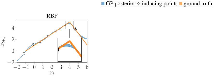
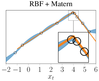
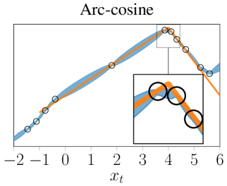
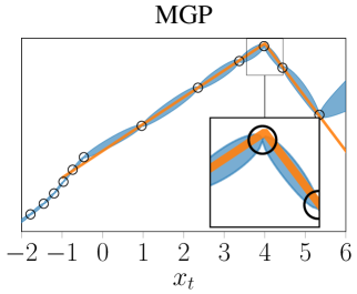
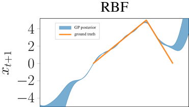
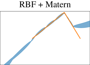
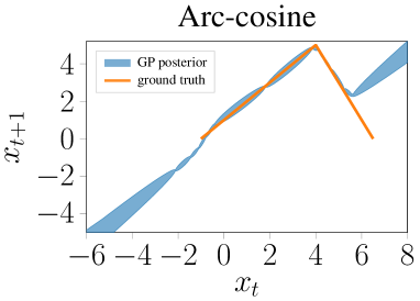
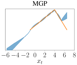
In our experiments, we set the system and measurement noise variances to $\sigma_{f}^{2}=0.01$ and $\sigma_{g}^{2}=0.1$, respectively, and generate 200 episodes of length $10$ that were used as the observed data for training the GPSSM. We used $20$ inducing points (initialised uniformly across the range of the input data) for approximating the GP and 20 hidden units for the recurrent recognition model. We evaluate the following kernels: RBF, additive composition of the RBF (initial $\ell=10$) and Matern ($\nu=\frac{1}{2}$, initial $\ell=0.1$), $0$-order arc-cosine (Cho and Saul, 2009), and the MGP kernel (Calandra et al., 2016) (depth 5, hidden dimensions $[3,2,3,2,3]$, $\tanh$ activation, Matern ($\nu=\frac{1}{2}$) compound kernel).

The learnt GP state transition functions are shown in Figure 2. With the non-smooth kernels we are able to learn accurate transitions and model the instantaneous dynamical change, as opposed to the smooth transition learnt with the RBF. Note that all non-smooth kernels place inducing points directly on the peak (at $x_{t}=4$) to model the kink, whereas the RBF kernel explains this behaviour as a longer-scale wiggliness of the posterior process. When using a kernel without the RBF component the GP posterior quickly reverts to the mean function ($\eta(x)=x$) as we move away from the data: the short length-scales that enable them to model the instantaneous change prevent them from extrapolating downwards in the transition function. The composition of the RBF and Matern kernel benefits from long and short length scales and can better extrapolate. The posteriors can be viewed across a longer range of the function space in the supplementary material.

Figure 2: The learnt state transition function with different kernels. The true function is given by eq. (16).

4.2 Modelling cart-pole dynamics

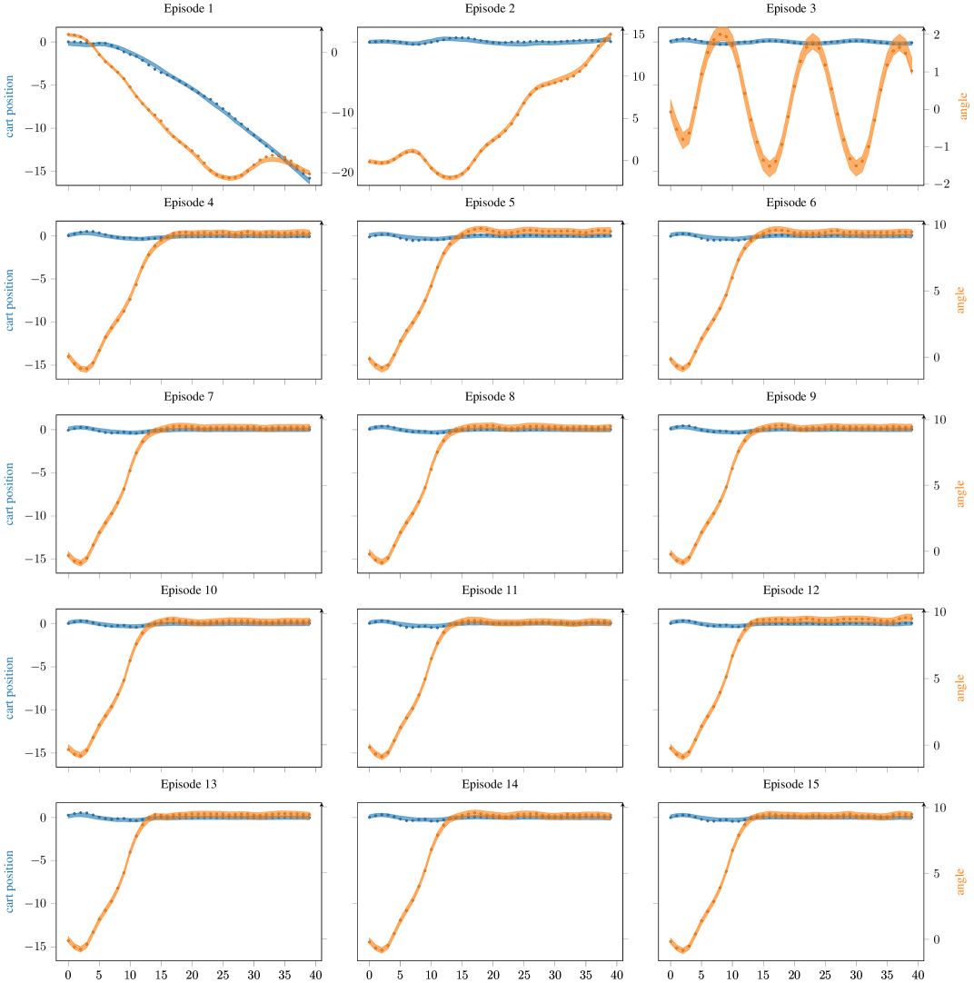
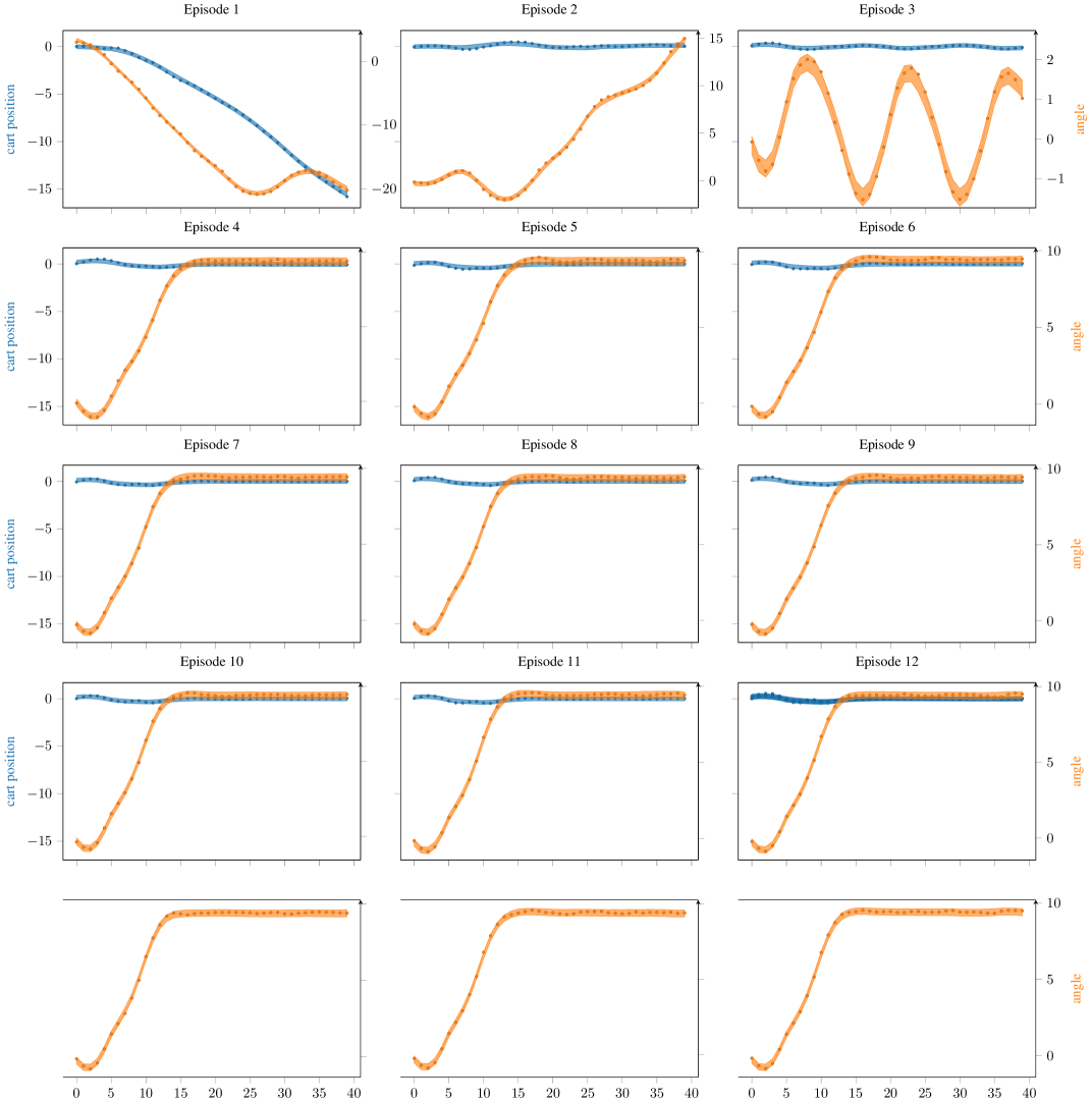
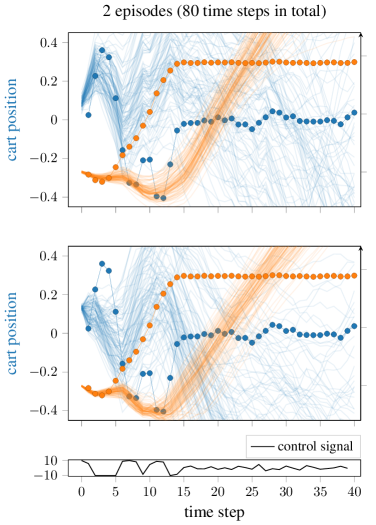
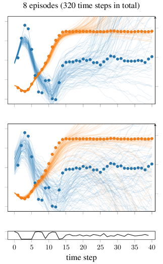
We demonstrate the efficacy of the proposed GPSSM on learning the non-linear dynamics of the cart-pole system from (Deisenroth and Rasmussen, 2011). The system is composed of a cart running on a track, with a freely swinging pendulum attached to it. The state of the system consists of the cart’s position and velocity, and the pendulum’s angle and angular velocity, while a horizontal force (action) $a\in[-10,10]N$ can be applied to the cart. We used the PILCO algorithm from (Deisenroth and Rasmussen, 2011) to learn a feedback controller that swings the pendulum and balances it in the inverted position in the middle of the track. We collected trajectory data from 16 trials during learning; each trajectory/episode was $4\,\mathrm{s}$ (40 time steps) long.

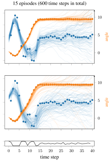
When training the GPSSM for the cart-pole system we used data up to the first 15 episodes. We used $100$ inducing points to approximate the GP function with a Matern $\nu=\frac{1}{2}$ and $50$ hidden units for the recurrent recognition model. The learning rate for the Adam optimiser was set to $10^{-3}$. We qualitatively assess the performance of our model by feeding the control sequence of the last episode to the GPSSM in order to generate future responses.

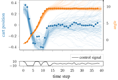
In Figure 3, we demonstrate the ability of the proposed GPSSM to learn the underlying dynamics of the system from a different number of episodes with fully and partially observed data. In the top row, the GPSSM observes the full 4D state, while in the bottom row, we train the GPSSM with only the cart’s position and the pendulum’s angle observed (i.e., the true state is not fully observed since the velocities are hidden). In both cases, sampling long-term trajectories based on only 2 episodes for training does not result in plausible future trajectories. However, we could model part of the dynamics after training with only 8 episodes (320 time steps interaction with the system), while training with 15 episodes (600 time steps in total) allowed the GPSSM to produce trajectories similar to the ground truth. It is worth emphasising the fact that the GPSSM could recover the unobserved velocities in the latent states, which resulted in smooth transitions of the cart and swinging of the pendulum. However, it seems that the recovered cart’s velocity is overestimated. This is evidenced by the increased variance in the prediction of the cart’s position around $0$ (the centre of the track). Detailed fittings for each episode and learnt latent states with observed and hidden velocities are provided in the supplementary material.

Figure 3: Predicting the cart’s position and pendulum’s angle behaviour from the cart-pole dataset by applying the control signal of the testing episode to sampled future trajectories from the proposed GPSSM. Learning of the dynamics is demonstrated with observed (upper row) and hidden (lower row) velocities and with increasing number of training episodes. Ground truth is denoted with the marked lines.

Table 1: Average Euclidean distance between the true and the predicted trajectories, measured at the pendulum’s tip. The error is in pendulum’s length units.

	2 episodes	8 episodes	15 episodes
Kalman	1.65	1.52	1.48
ARGP	1.22	1.03	0.80
GPSSM	1.21	0.67	0.59

Figure 4: Predictions with lagged actions.

In Table 1, we provide the average Euclidean distance between the predicted and the true trajectories measured at the pendulum’s tip, with fully observed states. We compare to two baselines: (i) the auto-regressive GP (ARGP) that maps the tuple $[{\boldsymbol{{y}}}_{t-1},a_{t-1}]$ to the next observation ${\boldsymbol{{y}}}_{t}$ (as in PILCO (Deisenroth et al., 2015)), and (ii) a linear system for identification that uses the Kalman filtering technique (Kalman, 1960). We see that the GPSSM significantly outperforms the baselines on this highly non-linear benchmark. The linear system cannot learn the dynamics at all, while the ARGP only manages to produce sensible error (less than a pendulum’s length) after seeing 15 episodes. Note that the GPSSM trained on 8 episodes produces trajectories with less error than the ARGP trained on 15 episodes.

We also ran experiments using lagged actions where the partially observed state at time $t$ is affected by the action at $t-2$. Figure 4 shows that we are able to sample future trajectories with an accuracy similar to time-aligned actions. This indicates that our model is able to learn a compressed representation of the full state and previous inputs, essentially ‘remembering’ the lagged actions.

4.3 Modelling double pendulum dynamics

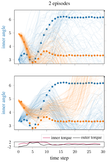
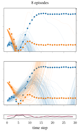
We demonstrate the learning and modelling of the dynamics of the double pendulum system from (Deisenroth et al., 2015). The double pendulum is a two-link robot arm with two actuators. The state of the system consists of the angles and the corresponding angular velocities of the inner and outer link, respectively, while different torques $a_{1},a_{2}\in[-2,2]\,\text{Nm}$ can be applied to the two actuators. The task of swinging the double pendulum and balancing it in the upwards position is extremely challenging. First, it requires the interplay of two correlated control signals (i.e., the torques). Second, the behaviour of the system, when operating at free will, is chaotic.

We learn the underlying dynamics from episodic data (15 episodes, 30 time steps long each). Training of the GPSSM was performed with data up to 14 episodes, while always demonstrating the learnt underlying dynamics on the last episode, which serves as the test set. We used $200$ inducing points to approximate the GP function with a Matern $\nu=\frac{1}{2}$ and $80$ hidden units for the recurrent recognition model. The learning rate for the Adam optimiser was set to $10^{-3}$. The difficulty of the task is evident in Figure 5, where we can see that even after observing 14 episodes we cannot accurately predict the system’s future behaviour for more than 15 time steps (i.e., $1.5\,\mathrm{s}$). It is worth noting that we can generate reliable simulation even though we observe only the pendulums’ angles.

Figure 5: Predicting the inner and outer pendulum’s angle from the double pendulum dataset by applying the control signals of the testing episode to sampled future trajectories from the proposed GPSSM. Learning of the dynamics is demonstrated with observed (upper row) and hidden (lower row) angular velocities and with increasing number of training episodes. Ground truth is denoted with the marked lines.

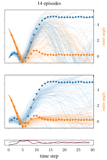
4.4 Modelling actuator dynamics

Here we evaluate the proposed GPSSM on real data from a hydraulic actuator that controls a robot arm (Sjöberg et al., 1995). The input is the size of the actuator’s valve opening and the output is its oil pressure. We train the GPSSM on half the sequence (512 steps) and evaluate the model on the remaining half. We use 15 inducing points to approximate the GP function with a combination of an RBF and a Matern $\nu=\frac{1}{2}$ and 15 hidden units for the recurrent recognition model. Figure 6 shows the fitting on the train data along with sampled future predictions from the learnt system when operating on a free simulation mode. It is worth noting the correct capturing of the uncertainty from the model at the points where the predictions are not accurate.

Figure 6: Demonstration of the identified model that controls the non-linear dynamics of the actuator dataset. The model’s fitting on the train data and sampled future predictions, after applying the control signal to the system. Ground truth is denoted with the marked lines.

5 Discussion and conclusion

We have proposed a novel inference mechanism for the GPSSM, in order to address the challenging task of non-linear system identification. Since our inference is based on the variational framework, successful learning of the model relies on defining good approximations to the posterior of the latent functions and states. Approximating the posterior over the dynamics with a sparse GP seems to be a reasonable choice given our assumptions over the transition function. However, the difficulty remains in the selection of the approximate posterior of the latent states. This is the key component that enables successful learning of the GPSSM.

In this work, we construct the variational posterior so that it follows the same Markov properties as the true states. Furthermore, it is enforced to have a simple-to-learn, linear, time-varying structure. To assure, though, that this approximation has rich representational capacity we proposed to recover the variational parameters of the posterior via a non-linear recurrent recognition model. Consequently, the joint approximate posterior resembles the behaviour of the true system, which facilitates the effective learning of the GPSSM.

In the experimental section we have provided evidence that the proposed approach is able to identify latent dynamics in true and simulated data, even from partial and lagged observations, while requiring only small data sets for this challenging task.

Acknowledgement

Marc P. Deisenroth has been supported by a Google faculty research award.

Appendix A Derivation of the ELBO

This appendix contains three parts: we first explicate the joint distribution of the model and data $p({\boldsymbol{{X}}},{\boldsymbol{{f}}}(\cdot),{\boldsymbol{{Y}}})$; then we describe the variational approximation to the model posterior $q({\boldsymbol{{X}}},{\boldsymbol{{f}}}(\cdot))$; then we show how they combine to produce the ELBO. Table 2 provides some nomenclature.

Table 2: Nomenclature used in this derivation

$t\in\{0\ldots T\}$	time steps indexed $t$
$d\in\{1\ldots D\}$	dimension of hidden states ${\boldsymbol{{x}}}_{t}$ indexed $d$
$O$	dimension of the observed data
$m\in\{1\ldots M\}$	number of inducing variables indexed $m$
${\boldsymbol{{x}}}_{t}$	hidden state at time $t$, ${\boldsymbol{{x}}}_{t}\in\mathbb{R}^{D}$
${\boldsymbol{{a}}}_{t}$	control input (action) at time $t$, ${\boldsymbol{{a}}}_{t}\in\mathbb{R}^{P}$
$\tilde{{\boldsymbol{{x}}}}_{t}$	concatenation of control input and state at $t$
${\boldsymbol{{y}}}_{t}$	observation at time $t$, ${\boldsymbol{{y}}}_{t}\in\mathbb{R}^{O}$
$\tilde{{\boldsymbol{{y}}}}_{t}$	concatenation of control input and observation at $t$
${\boldsymbol{{X}}}$	collection of hidden states, ${\boldsymbol{{X}}}=[{\boldsymbol{{x}}}_{t}]_{t=0}^{T}$.
${\boldsymbol{{Y}}}$	collection of observations, ${\boldsymbol{{Y}}}=[{\boldsymbol{{y}}}_{t}]_{t=0}^{T}$.
$\sigma^{2}_{f}$	variance of state transition noise
$\sigma^{2}_{g}$	variance of observation nosie
$f_{d}(\cdot)$	the $d^{\textrm{th}}$ Gaussian process (GP)
${\boldsymbol{{f}}}(\cdot)$	collection of GPs, $=[f_{d}(\cdot)]_{d=1}^{D}$
$\eta_{d}(\cdot)$	prior mean function of the $d^{\textrm{th}}$ GP
$k_{d}(\cdot\,,\cdot)$	prior covariance function of the $d^{\textrm{th}}$ GP
$\mu_{d}(\cdot)$	posterior mean function of the $d^{\textrm{th}}$ GP
$v_{d}(\cdot,\cdot)$	posterior covariance function of the $d^{\textrm{th}}$ GP
${\boldsymbol{{Z}}}$	Locations of variational pseudo-inputs
${\boldsymbol{{u}}}_{d}$	evaluations of the $d^{\textrm{th}}$ GP at the pseudo-inputs: ${\boldsymbol{{u}}}_{d}=[f_{d}({\boldsymbol{{z}}}_{m})]_{m=1}^{M}$.
${\boldsymbol{{U}}}$	collection: ${\boldsymbol{{U}}}=[{\boldsymbol{{u}}}_{d}]_{d=1}^{D}$
${\boldsymbol{{\mu}}}_{d}$	variational posterior mean of ${\boldsymbol{{u}}}_{d}$: ${\boldsymbol{{\mu}}}_{d}=[\mu_{d}({\boldsymbol{{z}}}_{m})]_{m=1}^{M}$
${\boldsymbol{{\Sigma}}}_{d}$	variational posterior covariance of ${\boldsymbol{{u}}}_{d}$
${\boldsymbol{{A}}}_{t}$	variational transition matrix of $q({\boldsymbol{{x}}}_{t}\,|\,{\boldsymbol{{x}}}_{t-1})$
${\boldsymbol{{L}}}_{t}$	triangular-square-root of variational covariance of $q({\boldsymbol{{x}}}_{t}\,|\,{\boldsymbol{{x}}}_{t-1})$
${\boldsymbol{{m}}}_{t}$	variational mean of the marginal $q({\boldsymbol{{x}}}_{t})$
${\boldsymbol{{S}}}_{t}$	variational covariance of the marginal $q({\boldsymbol{{x}}}_{t})$

A.1 Model joint distribution

Here we define the joint distribution of the Gaussian processes $f$, the latent states ${\boldsymbol{{x}}}$ and the data ${\boldsymbol{{y}}}$.

The Gaussian processes have prior mean $\eta(\cdot)$ and prior covariances $k(\cdot,\,\cdot)$:

$$p(f_{d}(\cdot))=\mathcal{GP}\big{(}\eta_{d}(\cdot),\,k_{d}(\cdot,\cdot)\big{)}\,\quad d=1\ldots D\,.$$ (17)

We note that placing a measure $p$ on the function $f$ causes some measure-theoretic discrepancies. Nonetheless, the derivation holds following a more theoretical consideration of the problem [Matthews et al., 2016], and the intuition given by our derivation is correct.

The initial state is assumed to be drawn from a standard normal distribution

$$p({\boldsymbol{{x}}}_{0})=\mathcal{N}({\boldsymbol{{0}}},\,{\boldsymbol{{I}}}_{D})\,.$$ (18)

The state transition depends on the Gaussian processes:

$$p({\boldsymbol{{x}}}_{t}\,|\,{\boldsymbol{{x}}}_{t-1},{\boldsymbol{{f}}}(\cdot))=\mathcal{N}\big{(}{\boldsymbol{{x}}}_{t}\,|\,{\boldsymbol{{f}}}(\tilde{{\boldsymbol{{x}}}}_{t-1}),\,\sigma_{f}^{2}{\boldsymbol{{I}}}_{D}\big{)}\,,$$ (19)

We assume a linear-Gaussian observation model:

$$p({\boldsymbol{{y}}}_{t}\,|\,{\boldsymbol{{x}}}_{t})=\mathcal{N}\big{(}{\boldsymbol{{y}}}_{t}\,|\,{\boldsymbol{{W}}}_{\!\!g}{\boldsymbol{{x}}}_{t}+{\boldsymbol{{b}}}_{g},\sigma_{g}^{2}{\boldsymbol{{I}}}_{O}\big{)}$$ (20)

The joint density is then

$$p({\boldsymbol{{f}}},{\boldsymbol{{X}}},{\boldsymbol{{Y}}})=\prod_{d=1}^{D}p(f_{d}(\cdot))\,p({\boldsymbol{{x}}}_{0})\,\prod_{t=1}^{T}p({\boldsymbol{{y}}}_{t}\,|\,{\boldsymbol{{x}}}_{t})\,\prod_{t=1}^{T}p({\boldsymbol{{x}}}_{t}\,|\,{\boldsymbol{{f}}},{\boldsymbol{{x}}}_{t-1})$$ (21)

A.2 Approximate posterior distribution

We will use variational Bayes to approximate the posterior distribution over ${\boldsymbol{{f}}}$ and ${\boldsymbol{{X}}}$, whilst simultaneously obtaining a bound on the marginal likelihood (the ELBO) which will be used to train the parameters of the model, including covariance function parameters, noise variances and the parameters ${\boldsymbol{{W}}}_{\!\!g},{\boldsymbol{{b}}}_{g}$ of the linear output mapping.

The posterior over Gaussian processes takes the form of a sparse GP. We introduce a series of $M$ variational inducing points ${\boldsymbol{{Z}}}=[{\boldsymbol{{z}}}_{m}]_{m=1}^{M}$ which lie in the same domain as $\tilde{{\boldsymbol{{x}}}}$. Following convention, the values of the $d^{\textrm{th}}$ function at those points are denoted ${\boldsymbol{{u}}}_{d}=[f_{d}({\boldsymbol{{z}}}_{m})]_{m=1}^{M}$, while evaluations from the prior as ${\boldsymbol{{\eta}}}_{d}=[\eta_{d}({\boldsymbol{{z}}}_{m})]_{m=1}^{M}$. Note that the variables ${\boldsymbol{{u}}}$ are not auxiliary variables, but part of the original model specification, being part of the GP. We assume a variational posterior of the form

$$q({\boldsymbol{{U}}})=\prod_{d=1}^{D}\mathcal{N}\big{(}{\boldsymbol{{u}}}_{d}\,|\,{\boldsymbol{{\mu}}}_{d},\,{\boldsymbol{{\Sigma}}}_{d}\big{)}\,.$$ (22)

The remainder of the GPs conditioned on ${\boldsymbol{{u}}}$ are assumed to take the same form as the GP prior conditional. That is

$$q(f_{d}(\cdot)\,|\,{\boldsymbol{{u}}}_{d})=p(f_{d}(\cdot)\,|\,{\boldsymbol{{u}}}_{d})=\mathcal{G}P\big{(}\eta_{d}(\cdot)+k(\cdot,{\boldsymbol{{Z}}}){\boldsymbol{{K}}}_{zz}^{-1}({\boldsymbol{{u}}}_{d}-{\boldsymbol{{\eta}}}_{d}),\,k(\cdot,\cdot)-k(\cdot,{\boldsymbol{{Z}}}){\boldsymbol{{K}}}_{zz}^{-1}k({\boldsymbol{{Z}}},\cdot)\big{)}\,.$$ (23)

Marginalising with respect to ${\boldsymbol{{u}}}_{d}$ leads to our approximation to the GP:

$$q(f_{d}(\cdot))=\mathcal{GP}\big{(}\mu_{d}(\cdot),v_{d}(\cdot,\cdot)\big{)}\,,$$ (24)

with

$$\mu_{d}(\cdot) =\eta_{d}(\cdot)+k(\cdot,{\boldsymbol{{Z}}}){\boldsymbol{{K}}}_{zz}^{-1}({\boldsymbol{{\mu}}}_{d}-{\boldsymbol{{\eta}}}_{d})\,,$$ (25)

$$v_{d}(\cdot,\cdot) =k(\cdot,\cdot)-k(\cdot,{\boldsymbol{{Z}}}){\boldsymbol{{K}}}_{zz}^{-1}[{\boldsymbol{{K}}}_{zz}-{\boldsymbol{{\Sigma}}}_{d}]{\boldsymbol{{K}}}_{zz}^{-1}k({\boldsymbol{{Z}}},\cdot)\,.$$ (26)

The approximation to the posterior over state trajectories is given a Gauss-Markov structure of the form

$$q({\boldsymbol{{X}}})=q({\boldsymbol{{x}}}_{0})\prod_{t=1}^{T}q({\boldsymbol{{x}}}_{t}\,|\,{\boldsymbol{{x}}}_{t-1})\,,$$ (27)

where

$$q({\boldsymbol{{x}}}_{0}) =\mathcal{N}({\boldsymbol{{x}}}_{0}\,|\,{\boldsymbol{{m}}}_{0},\,{\boldsymbol{{L}}}_{0}{\boldsymbol{{L}}}_{0}^{\top})$$ (28)

$$q({\boldsymbol{{x}}}_{t}\,|\,{\boldsymbol{{x}}}_{t-1}) =\mathcal{N}({\boldsymbol{{x}}}_{t}\,|\,{\boldsymbol{{A}}}_{t}{\boldsymbol{{x}}}_{t-1},\,{\boldsymbol{{L}}}_{t}{\boldsymbol{{L}}}_{t}^{\top})\,.$$ (29)

The complete set of variational parameters is then ${\boldsymbol{{Z}}},\{{\boldsymbol{{\mu}}}_{d},{\boldsymbol{{\Sigma}}}_{d}\}_{d=1}^{D},{\boldsymbol{{m}}}_{0},{\boldsymbol{{L}}}_{0},\{{\boldsymbol{{A}}}_{t},{\boldsymbol{{L}}}_{t}\}_{t=1}^{T}$. The parameters of $q({\boldsymbol{{X}}})$ are reconfigured to be the output of an RNN recognition model (see main text), whilst we optimise the parameters controlling ${\boldsymbol{{f}}}(\cdot)$ directly.

The joint posterior then factors as

$$q({\boldsymbol{{f}}}(\cdot),{\boldsymbol{{X}}})=\prod_{d=1}^{D}q(f_{d}(\cdot))q({\boldsymbol{{X}}})\,.$$ (30)

A.3 The ELBO

Having specified the forms of the model and the approximate posterior, we are ready to derive the ELBO. Following the standard variational Bayes methods, we write

$$\textsc{ELBO}=\mathbb{E}_{q({\boldsymbol{{X}}})q({\boldsymbol{{f}}}(\cdot))}\left[\log\frac{p({\boldsymbol{{Y}}}\,|\,{\boldsymbol{{X}}})p({\boldsymbol{{X}}}\,|\,{\boldsymbol{{f}}}(\cdot))}{q({\boldsymbol{{X}}})}\frac{p({\boldsymbol{{f}}}(\cdot))}{q({\boldsymbol{{f}}}(\cdot))}\right]\,.$$ (31)

We will split the ELBO into four parts, dealing with each in turn:

$$\textsc{ELBO}= \underbrace{\mathbb{E}_{q({\boldsymbol{{X}}})}\big{[}\log p({\boldsymbol{{Y}}}\,|\,{\boldsymbol{{X}}})\big{]}}_{\text{part 1}}+\underbrace{\mathbb{E}_{q({\boldsymbol{{X}}})q({\boldsymbol{{f}}}(\cdot))}\big{[}\log p({\boldsymbol{{X}}}\,|\,{\boldsymbol{{f}}}(\cdot))\big{]}}_{\text{part 2}}$$

$$-\underbrace{\mathbb{E}_{q({\boldsymbol{{X}}})}\big{[}\log q({\boldsymbol{{X}}})\big{]}}_{\text{part 3}}+\underbrace{\mathbb{E}_{q({\boldsymbol{{f}}}(\cdot))}\big{[}\log\frac{p({\boldsymbol{{f}}}(\cdot))}{q({\boldsymbol{{f}}}(\cdot))}\big{]}}_{\text{part 4}}\,.$$ (32)

Part 1

This expression can be computed straight-forwardly in closed form due to our choice of a linear-Gaussian emission $g({\boldsymbol{{x}}})$. Let ${\boldsymbol{{m}}}_{t},{\boldsymbol{{\Sigma}}}_{t}$ be the marginals of $q({\boldsymbol{{x}}}_{t})$ computed via the recursion, and recall the form of the linear emission function $g({\boldsymbol{{x}}}_{t})={\boldsymbol{{W}}}_{\!\!g}{\boldsymbol{{x}}}_{t}+{\boldsymbol{{b}}}_{g}$

$$\mathbb{E}_{q({\boldsymbol{{X}}})}\big{[}\log p({\boldsymbol{{Y}}}\,|\,{\boldsymbol{{X}}})\big{]} =\mathbb{E}_{q({\boldsymbol{{X}}})}\Big{[}\sum_{t=1}^{T}\log\mathcal{N}\big{(}{\boldsymbol{{y}}}_{t}\,|\,g({\boldsymbol{{x}}}_{t}),\sigma^{2}_{g}\big{)}\Big{]}$$

$$=\sum_{t=1}^{T}\mathbb{E}_{q({\boldsymbol{{x}}}_{t})}\Big{[}\log\mathcal{N}\big{(}{\boldsymbol{{y}}}_{t}\,|\,{\boldsymbol{{W}}}_{\!\!g}{\boldsymbol{{x}}}_{t}+{\boldsymbol{{b}}}_{g},\sigma^{2}_{g}\big{)}\Big{]}$$

$$=\sum_{t=1}^{T}\log\mathcal{N}\big{(}{\boldsymbol{{y}}}_{t}\,|\,{\boldsymbol{{W}}}_{\!\!g}{\boldsymbol{{m}}}_{t}+{\boldsymbol{{b}}}_{g},\sigma^{2}_{g}\big{)}-\tfrac{1}{2\sigma^{2}_{n}}\textrm{tr}({\boldsymbol{{W}}}_{\!\!g}^{\top}{\boldsymbol{{W}}}_{\!\!g}{\boldsymbol{{\Sigma}}}_{t})\,.$$ (33)

In practise we defer this simple computation to the variational_expectations functionality in GPflow [Matthews et al., 2017].

Part 2

This expression cannot be computed in closed form without restriction to the RBF kernel as in [Frigola, 2015]. We eliminate the integral with respect to ${\boldsymbol{{f}}}$ here, and then use the reparameterisation trick to estimate the integral with respect to ${\boldsymbol{{X}}}$ (see main text).

part 2 $$=\mathbb{E}_{q({\boldsymbol{{X}}})q({\boldsymbol{{f}}}(\cdot))}\big{[}\log p({\boldsymbol{{X}}}\,|\,{\boldsymbol{{f}}}(\cdot))\big{]}$$

$$=\mathbb{E}_{q({\boldsymbol{{X}}})q({\boldsymbol{{f}}}(\cdot))}\big{[}\log p({\boldsymbol{{x}}}_{0})\prod_{t=1}^{T}\mathcal{N}\big{(}{\boldsymbol{{x}}}_{t}\,|\,{\boldsymbol{{f}}}(\tilde{{\boldsymbol{{x}}}}_{t-1}),\,\sigma_{f}^{2}{\boldsymbol{{I}}}_{D}\big{)}\big{]}$$

$$=\mathbb{E}_{q({\boldsymbol{{x}}}_{0})}\big{[}\log p({\boldsymbol{{x}}}_{0})\big{]}+\mathbb{E}_{q({\boldsymbol{{X}}})q({\boldsymbol{{f}}}(\cdot))}\Big{[}\sum_{t=1}^{T}\sum_{d=1}^{D}\log\mathcal{N}\big{(}{\boldsymbol{{x}}}_{t}^{(d)}\,|\,f_{d}(\tilde{{\boldsymbol{{x}}}}_{t-1}),\,\sigma_{f}^{2}\big{)}\Big{]}$$

$$=\mathbb{E}_{q({\boldsymbol{{x}}}_{0})}\big{[}\log p({\boldsymbol{{x}}}_{0})\big{]}+\mathbb{E}_{q({\boldsymbol{{X}}})}\Big{[}\sum_{t=1}^{T}\sum_{d=1}^{D}\log\mathcal{N}\big{(}{\boldsymbol{{x}}}_{t}^{(d)}\,|\,\mu_{d}(\tilde{{\boldsymbol{{x}}}}_{t-1}),\,\sigma_{f}^{2}\big{)}-\tfrac{1}{2}\sigma_{f}^{-2}v_{d}(\tilde{{\boldsymbol{{x}}}}_{t-1},\tilde{{\boldsymbol{{x}}}}_{t-1})\Big{]},$$ (34)

which matches the term in the main text.

Part 3

This corresponds to the entropy of $q({\boldsymbol{{X}}})$. It is straightforward to derive:

$$-\mathbb{E}_{q({\boldsymbol{{X}}})}\big{[}\log q({\boldsymbol{{X}}})\big{]}=\textsc{H}[q({\boldsymbol{{X}}})]=\frac{(T+1)D}{2}\log(2\pi e)+\sum_{t=0}^{T}\log(\det({\boldsymbol{{L}}}_{t}))\,.$$ (35)

Part 4

This final part is the Kullback-Leibler divergence between the prior and (approximate) posterior GPs. We first note that it can be written as a sum across dimensions $d$, and then that each GP $f_{d}(\cdot)$ can be factored into two parts: $p(f_{d}(\cdot)\,|\,{\boldsymbol{{u}}}_{d})p({\boldsymbol{{u}}}_{d})$ and similarly for $q$. This results in

$$\mathbb{E}_{q({\boldsymbol{{f}}}(\cdot))}\left[\log\frac{p({\boldsymbol{{f}}}(\cdot))}{q({\boldsymbol{{f}}}(\cdot))}\right] =\sum_{d=1}^{D}\mathbb{E}_{q(f_{d}(\cdot))}\left[\log\frac{p(f_{d}(\cdot))}{q(f_{d}(\cdot))}\right]$$

$$=\sum_{d=1}^{D}\mathbb{E}_{q(f_{d}(\cdot)\,|\,{\boldsymbol{{u}}}_{d})q({\boldsymbol{{u}}}_{d})}\left[\log\frac{p(f_{d}(\cdot)\,|\,{\boldsymbol{{u}}}_{d})p({\boldsymbol{{u}}}_{d})}{q(f_{d}(\cdot)\,|\,{\boldsymbol{{u}}}_{d})q({\boldsymbol{{u}}}_{d})}\right]\,.$$ (36)

Since we have defined the posterior conditional $q(f_{d}(\cdot)\,|\,{\boldsymbol{{u}}}_{d}$) to match the prior conditional, the two terms cancel, resulting in

$$\mathbb{E}_{q({\boldsymbol{{f}}}(\cdot))}\left[\log\frac{p({\boldsymbol{{f}}}(\cdot))}{q({\boldsymbol{{f}}}(\cdot))}\right] =\sum_{d=1}^{D}\mathbb{E}_{q({\boldsymbol{{u}}}_{d})}\left[\log\frac{p({\boldsymbol{{u}}}_{d})}{q({\boldsymbol{{u}}}_{d})}\right]$$

$$=-\sum_{d=1}^{D}\textsc{KL}\big{[}q({\boldsymbol{{u}}}_{d})||p({\boldsymbol{{u}}}_{d})\big{]}\,.$$ (37)

Since the result is a Kullback-Leibler divergence between two finite-dimensional normal distributions, it is computed straightforwardly.

Although this notation is somewhat sloppy (since the sets of variables $f_{d}(\cdot)$ and ${\boldsymbol{{u}}}_{d}$ overlap), the result is correct. Matthews [2017] contains a more careful and significantly more technical derivation.

Appendix B Full visualisation of synthetic 1D dataset

Figure 7: Visualisation of the learned GP transition functions across a greater domain of the function. It can be seen that all models revert to the mean function (defined as the identity function) away from the data. The short lengthscales of the Arc-cosine and MGP (compounded with a Matern kernel) that are used to fit the kink of the true transition function mean that they almost instantaneously revert to the mean function. The longer length scales of the RBF-containing kernels mean that we revert much more slowly to the mean.

Appendix C Learnt latent states for cart-pole

Below we provide the learnt latent states for the cart-pole dataset with observed and hidden velocities. It is worth noting that the model has recovered similar structure for both cases.

Figure 8: Learnt latent states for the cart-pole dataset with observed velocities.

Figure 9: Learnt latent states for the cart-pole dataset with hidden velocities.

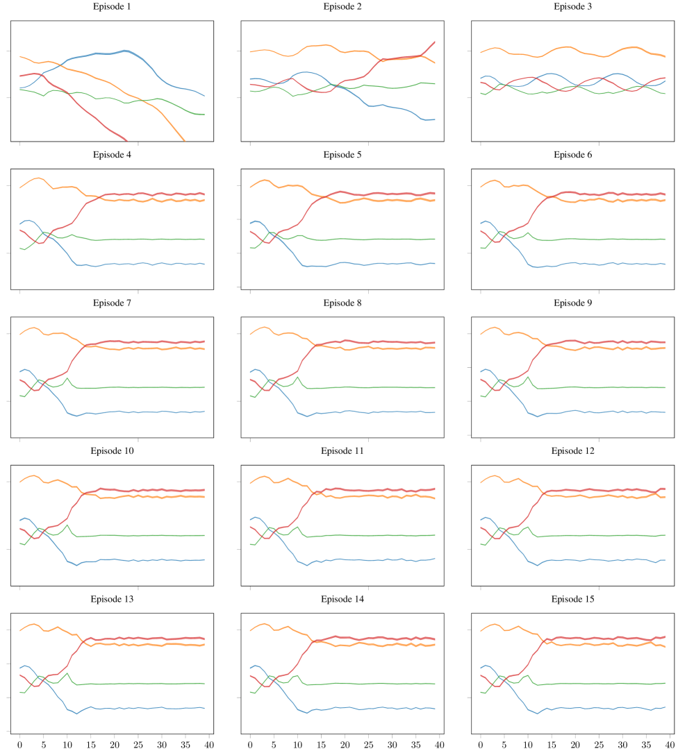
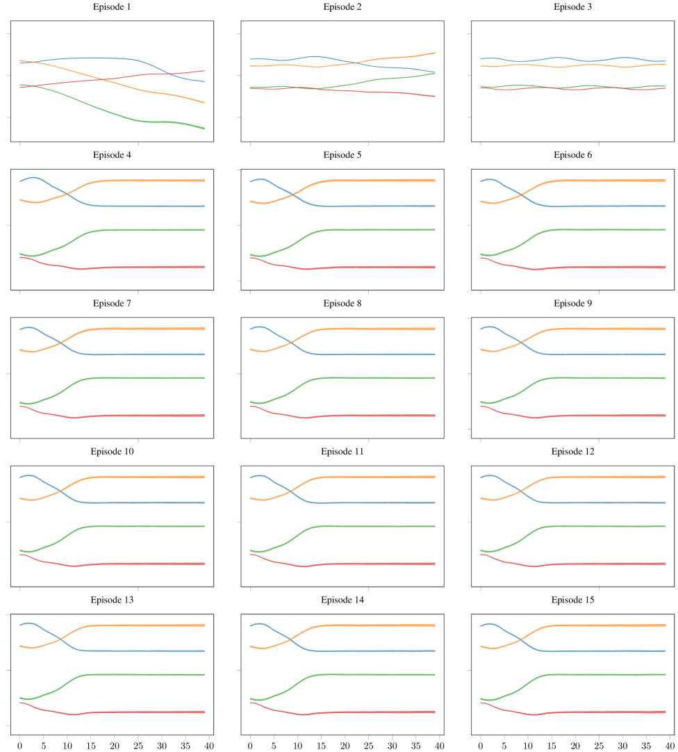
Appendix D Cart-pole training data fitting

Below we provide detailed fittings on the training episodes for the cart-pole dataset.

Figure 10: Detailed fittings per episode for the cart-pole dataset with observed velocities.

Figure 11: Detailed fittings per episode for the cart-pole dataset with hidden velocities.

References

- Al-Shedivat et al. [2016] Maruan Al-Shedivat, Andrew G. Wilson, Yunus Saatchi, Zhiting Hu, and Eric P. Xing. Learning scalable deep kernels with recurrent structure. arXiv preprint arXiv:1610.08936, 2016.
- Beal [2003] Matthew J. Beal. Variational algorithms for approximate Bayesian inference. PhD thesis, University of London, London, UK, 2003.
- Blei et al. [2017] David M. Blei, Alp Kucukelbir, and Jon D. McAuliffe. Variational inference: A review for statisticians. Journal of the American Statistical Association, 112(518):859–877, 2017.
- Brown et al. [1998] Emery N. Brown, Loren M. Frank, Dengda Tang, Michael C. Quirk, and Matthew A. Wilson. A statistical paradigm for neural spike train decoding applied to position prediction from ensemble firing patterns of rat hippocampal place cells. Journal of Neuroscience, 18(18):7411–7425, 1998.
- Calandra et al. [2016] Roberto Calandra, Jan Peters, Carl E. Rasmussen, and Marc P. Deisenroth. Manifold Gaussian processes for regression. In IEEE International Joint Conference on Neural Networks, 2016.
- Cho et al. [2014] KyungHyun Cho, Bart van Merrienboer, Dzmitry Bahdanau, and Yoshua Bengio. On the properties of neural machine translation: Encoder-decoder approaches. arXiv preprint arXiv:1409.1259, 2014.
- Cho and Saul [2009] Youngmin Cho and Lawrence K. Saul. Kernel methods for deep learning. In Advances in Neural Information Processing Systems, pages 342–350. 2009.
- Dai et al. [2015] Zhenwen Dai, Andreas Damianou, Javier González, and Neil Lawrence. Variational auto-encoded deep Gaussian processes. In International Conference on Learning Representations, 2015.
- Deisenroth and Mohamed [2012] Marc P. Deisenroth and Shakir Mohamed. Expectation propagation in Gaussian process dynamical systems. In Advances in Neural Information Processing Systems, pages 2618–2626, 2012.
- Deisenroth and Rasmussen [2011] Marc P. Deisenroth and Carl E. Rasmussen. PILCO: A model-based and data-efficient approach to policy search. In International Conference on Machine Learning, pages 465–472, 2011.
- Deisenroth et al. [2009] Marc P. Deisenroth, Marco F. Huber, and Uwe D. Hanebeck. Analytic moment-based Gaussian process filtering. In International Conference on Machine Learning, pages 225–232, 2009.
- Deisenroth et al. [2012] Marc P. Deisenroth, Ryan D. Turner, Marco Huber, Uwe D. Hanebeck, and Carl E. Rasmussen. Robust filtering and smoothing with Gaussian processes. IEEE Transactions on Automatic Control, 57(7):1865–1871, 2012.
- Deisenroth et al. [2015] Marc P. Deisenroth, Dieter Fox, and Carl E. Rasmussen. Gaussian processes for data-efficient learning in robotics and control. IEEE Transactions on Pattern Analysis and Machine Intelligence, 37(2):408–423, 2015.
- Frigola [2015] Roger Frigola. Bayesian time series learning with Gaussian processes. PhD thesis, University of Cambridge, Cambridge, UK, 2015.
- Frigola et al. [2013] Roger Frigola, Fredrik Lindsten, Thomas B. Schön, and Carl E. Rasmussen. Bayesian inference and learning in Gaussian process state-space models with particle MCMC. In Advances in Neural Information Processing Systems, pages 3156–3164, 2013.
- Frigola et al. [2014] Roger Frigola, Yutian Chen, and Carl E. Rasmussen. Variational Gaussian process state-space models. In Advances in Neural Information Processing Systems, pages 3680–3688, 2014.
- Kalman [1960] Rudolf E. Kalman. A new approach to linear filtering and prediction problems. Transactions of the American Society of Mathematical Engineering, Journal of Basic Engineering, 82(D):35–45, 1960.
- Kingma and Ba [2015] Diederik P. Kingma and Jimmy Ba. Adam: A method for stochastic optimization. In International Conference on Learning Representations, 2015.
- Kingma and Welling [2014] Diederik P. Kingma and Max Welling. Auto-encoding variational Bayes. In International Conference on Learning Representations, 2014.
- Ko and Fox [2009a] Jonathan Ko and Dieter Fox. GP-BayesFilters: Bayesian filtering using Gaussian process prediction and observation models. Autonomous Robots, 27(1):75–90, 2009a.
- Ko and Fox [2009b] Jonathan Ko and Dieter Fox. Learning GP-BayesFilters via Gaussian process latent variable models. In Robotics: Science and Systems, 2009b.
- Kocijan [2016] Juš Kocijan. Modelling and control of dynamic systems using Gaussian process models. Springer, 2016.
- Likar and Kocijan [2007] Bojan Likar and Juš Kocijan. Predictive control of a gas-liquid separation plant based on a Gaussian process model. Computers & Chemical Engineering, 31(3):142–152, 2007.
- Ljung [1999] Lennart Ljung. System identification: Theory for the user. Prentice Hall, 1999.
- Matthews [2017] Alexander G. de G. Matthews. Scalable Gaussian process inference using variational methods. PhD thesis, University of Cambridge, Cambridge, UK, 2017.
- Matthews et al. [2016] Alexander G. de G. Matthews, James Hensman, Richard E. Turner, and Zoubin Ghahramani. On sparse variational methods and the Kullback-Leibler divergence between stochastic processes. In International Conference on Artificial Intelligence and Statistics, volume 51 of JMLR W&CP, pages 231–239, 2016.
- Matthews et al. [2017] Alexander G. de G. Matthews, Mark van der Wilk, Tom Nickson, Keisuke Fujii, Alexis Boukouvalas, Pablo León-Villagrá, Zoubin Ghahramani, and James Hensman. GPflow: A Gaussian process library using TensorFlow. Journal of Machine Learning Research, 18(40):1–6, 2017.
- Mattos et al. [2015] César Lincoln C. Mattos, Zhenwen Dai, Andreas Damianou, Jeremy Forth, Guilherme A. Barreto, and Neil D. Lawrence. Recurrent Gaussian processes. In International Conference on Learning Representations, 2015.
- Murray-Smith and Girard [2001] Roderick Murray-Smith and Agathe Girard. Gaussian process priors with ARMA noise models. In Irish Signals and Systems Conference, pages 147–152, 2001.
- Rasmussen and Williams [2006] Carl E. Rasmussen and Christopher K. I. Williams. Gaussian processes for machine learning. The MIT Press, Cambridge, MA, USA, 2006.
- Rezende et al. [2014] Danilo J. Rezende, Shakir Mohamed, and Daan Wierstra. Stochastic backpropagation and approximate inference in deep generative models. In International Conference on Machine Learning, pages 1278–1286, 2014.
- Roberts et al. [2013] Stephen Roberts, Michael Osborne, Mark Ebden, Steven Reece, Neale Gibson, and Suzanne Aigrain. Gaussian processes for time-series modelling. Philosophical Transactions of the Royal Society A, 371(1984):20110550, 2013.
- Schneider [1997] Jeff G. Schneider. Exploiting model uncertainty estimates for safe dynamic control learning. In Advances in Neural Information Processing Systems. 1997.
- Sjöberg et al. [1995] Jonas Sjöberg, Qinghua Zhang, Lennart Ljung, Albert Benveniste, Bernard Delyon, Pierre-Yves Glorennec, Håkan Hjalmarsson, and Anatoli Juditsky. Nonlinear black-box modeling in system identification: A unified overview. Automatica, 31(12):1691–1724, 1995.
- Titsias [2009] Michalis K. Titsias. Variational learning of inducing variables in sparse Gaussian processes. In International Conference on Artificial Intelligence and Statistics, volume 5 of JMLR W&CP, pages 567–574, 2009.
- Titsias and Lawrence [2010] Michalis K. Titsias and Neil D. Lawrence. Bayesian Gaussian process latent variable model. In International Conference on Artificial Intelligence and Statistics, volume 9 of JMLR W&CP, pages 844–851, 2010.
- Titsias and Lázaro-Gredilla [2014] Michalis K. Titsias and Miguel Lázaro-Gredilla. Doubly stochastic variational Bayes for non-conjugate inference. In International Conference on Machine Learning, pages 1971–1979, 2014.
- Turner [2011] Ryan D. Turner. Gaussian processes for state space models and change point detection. PhD thesis, University of Cambridge, Cambridge, UK, 2011.
- Turner et al. [2010] Ryan D. Turner, Marc P. Deisenroth, and Carl E. Rasmussen. State-space inference and learning with Gaussian processes. In International Conference on Artificial Intelligence and Statistics, volume 9 of JMLR W&CP, pages 868–875, 2010.
- Wang et al. [2008] Jack M. Wang, David J. Fleet, and Aaron Hertzmann. Gaussian process dynamical models for human motion. IEEE Transactions on Pattern Analysis and Machine Intelligence, 30(2):283–298, 2008.