Working hard to know your neighbor’s margins:
Local descriptor learning loss

Abstract

We introduce a loss for metric learning, which is inspired by the Lowe’s matching criterion for SIFT. We show that the proposed loss, that maximizes the distance between the closest positive and closest negative example in the batch, is better than complex regularization methods; it works well for both shallow and deep convolution network architectures. Applying the novel loss to the L2Net CNN architecture results in a compact descriptor named HardNet. It has the same dimensionality as SIFT (128) and shows state-of-art performance in wide baseline stereo, patch verification and instance retrieval benchmarks.

1 Introduction

Many computer vision tasks rely on finding local correspondences, e.g. image retrieval [1, 2], panorama stitching [3], wide baseline stereo [4], 3D-reconstruction [5, 6]. Despite the growing number of attempts to replace complex classical pipelines with end-to-end learned models, e.g., for image matching [7], camera localization [8], the classical detectors and descriptors of local patches are still in use, due to their robustness, efficiency and their tight integration. Moreover, reformulating the task, which is solved by the complex pipeline as a differentiable end-to-end process is highly challenging.

As a first step towards end-to-end learning, hand-crafted descriptors like SIFT [9, 10] or detectors [9, 11, 12] have been replace with learned ones, e.g., LIFT [13], MatchNet [14] and DeepCompare [15]. However, these descriptors have not gained popularity in practical applications despite good performance in the patch verification task. Recent studies have confirmed that SIFT and its variants (RootSIFT-PCA [16], DSP-SIFT [17]) significantly outperform learned descriptors in image matching and small-scale retrieval [18], as well as in 3D-reconstruction [19]. One of the conclusions made in [19] is that current local patches datasets are not large and diverse enough to allow the learning of a high-quality widely-applicable descriptor.

In this paper, we focus on descriptor learning and, using a novel method, train a convolutional neural network (CNN), called HardNet. We additionally show that our learned descriptor significantly outperforms both hand-crafted and learned descriptors in real-world tasks like image retrieval and two view matching under extreme conditions. For the training, we use the standard patch correspondence data thus showing that the available datasets are sufficient for going beyond the state of the art.

2 Related work

Classical SIFT local feature matching consists of two parts: finding nearest neighbors and comparing the first to second nearest neighbor distance ratio threshold for filtering false positive matches. To best of our knowledge, no work in local descriptor learning fully mimics such strategy as the learning objective.

Simonyan and Zisserman [20] proposed a simple filter plus pooling scheme learned with convex optimization to replace the hand-crafted filters and poolings in SIFT. Han et al. [14] proposed a two-stage siamese architecture – for embedding and for two-patch similarity. The latter network improved matching performance, but prevented the use of fast approximate nearest neighbor algorithms like kd-tree [21]. Zagoruyko and Komodakis [15] have independently presented similar siamese-based method which explored different convolutional architectures. Simo-Serra et al [22] harnessed hard-negative mining with a relative shallow architecture that exploited pair-based similarity.

The three following papers have most closedly followed the classical SIFT matching scheme. Balntas et al [23] used a triplet margin loss and a triplet distance loss, with random sampling of the patch triplets. They show the superiority of the triplet-based architecture over a pair based. Although, unlike SIFT matching or our work, they sampled negatives randomly. Choy et al [7] calculate the distance matrix for mining positive as well as negative examples, followed by pairwise contrastive loss.

Tian et al [24] use $n$ matching pairs in batch for generating $n^{2}-n$ negative samples and require that the distance to the ground truth matchings is minimum in each row and column. No other constraint on the distance or distance ratio is enforced. Instead, they propose a penalty for the correlation of the descriptor dimensions and adopt deep supervision [25] by using intermediate feature maps for matching. Given the state-of-art performance, we have adopted the L2Net [24] architecture as base for our descriptor. We show that it is possible to learn even more powerful descriptor with significantly simpler learning objective without need of the two auxiliary loss terms.

Figure 1: Proposed sampling procedure. First, patches are described by the current network, then a distance matrix is calculated. The closest non-matching descriptor – shown in red – is selected for each $a_{i}$ and $p_{i}$ patch from positive pair (green) respectively. Finally, among two negative candidates the hardest one is chosen. All operations are done in a single forward pass.

3 The proposed descriptor

3.1 Sampling and loss

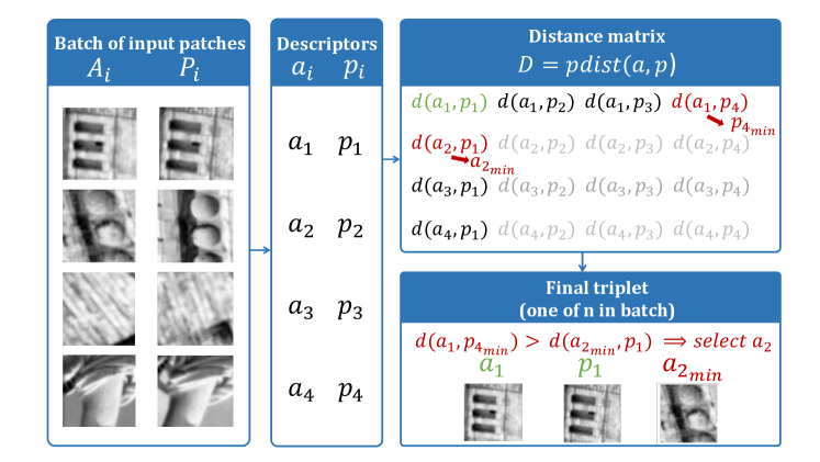
Our learning objective mimics SIFT matching criterion. The process is shown in Figure 1. First, a batch $\mathcal{X}=(A_{i},P_{i})_{i=1..n}$ of matching local patches is generated, where $A$ stands for the anchor and $P$ for the positive. The patches $A_{i}$ and $P_{i}$ correspond to the same point on 3D surface. We make sure that in batch $\mathcal{X}$, there is exactly one pair originating from a given 3D point.

Second, the $2n$ patches in $\mathcal{X}$ are passed through the network shown in Figure 2.

L2 pairwise distance matrix $D=\text{cdist}(a,p)$, where, $d(a_{i},p_{j})=\sqrt{2-2a_{i}p_{j}}$, $i=1..n,j=1..n$ of size $n\times n$ is calculated, where $a_{i}$ and $p_{j}$ denote the descriptors of patches $A_{i}$ and $P_{j}$ respectively.

Next, for each matching pair $a_{i}$ and $p_{i}$ the closest non-matching descriptors i.e. the $2^{nd}$ nearest neighbor, are found respectively:

$a_{i}$ – anchor descriptor, $p_{i}$ – positive descriptor,

$p_{j_{min}}$ – closest non-matching descriptor to $a_{i}$, where $j_{min}=\operatorname*{arg\,min}_{j=1..n,j\neq i}{d(a_{i},p_{j})}$,

$a_{k_{min}}$ – closest non-matching descriptor to $p_{i}$ where $k_{min}=\operatorname*{arg\,min}_{k=1..n,k\neq i}{d(a_{k},p_{i})}$.

Then from each quadruplet of descriptors $(a_{i},p_{i},p_{j_{min}},a_{k_{min}})$, a triplet is formed: $(a_{i},p_{i},p_{j_{min}})$, if $d(a_{i},p_{j_{min}})<d(a_{k_{min}},p_{i})$ and $(p_{i},a_{i},a_{k_{min}})$ otherwise.

Our goal is to minimize the distance between the matching descriptor and closest non-matching descriptor. These $n$ triplet distances are fed into the triplet margin loss:

$$L=\frac{1}{n}\sum_{i=1,n}{\max{(0,1+d(a_{i},p_{i})-\min{(d(a_{i},p_{j_{min}}),d(a_{k_{min}},p_{i}))})}}$$ (1)

where $\min{(d(a_{i},p_{j_{min}}),d(a_{k_{min}},p_{i})}$ is pre-computed during the triplet construction.

The distance matrix calculation is done on GPU and the only overhead compared to the random triplet sampling is the distance matrix calculation and calculating the minimum over rows and columns. Moreover, compared to usual learning with triplets, our scheme needs only two-stream CNN, not three, which results in 30% less memory consumption and computations.

Unlike in [24], neither deep supervision for intermediate layers is used, nor a constraint on the correlation of descriptor dimensions. We experienced no significant over-fitting.

3.2 Model architecture

Figure 2: The architecture of our network, adopted from L2Net [24]. Each convolutional layer is followed by batch normalization and ReLU, except the last one. Dropout regularization is used before the last convolution layer.

The HardNet architecture, Figure 2, is identical to L2Net [24]. Padding with zeros is applied to all convolutional layers, to preserve the spatial size, except to the final one. There are no pooling layers, since we found that they decrease performance of the descriptor. That is why the spatial size is reduced by strided convolutions. Batch normalization [26] layer followed by ReLU [27] non-linearity is added after each layer, except the last one. Dropout [28] regularization with 0.1 dropout rate is applied before the last convolution layer. The output of the network is L2 normalized to produce 128-D descriptor with unit-length. Grayscale input patches with size $32\times 32$ pixels are normalized by subtracting the per-patch mean and dividing by the per-patch standard deviation.

Optimization is done by stochastic gradient descent with learning rate of 0.1, momentum of 0.9 and weight decay of 0.0001. Learning rate was linearly decayed to zero within 10 epochs for the most of the experiments in this paper. Weights were initialized to orthogonally [29] with gain equal to 0.6, biases set to 0.01 Training is done with PyTorch library [30].

Post-NIPS update. After two major updates of PyTorch library, we were not able to reproduce the results. Therefore, we did a hyperparameter search and we found that increasing the learning rate to 10 and dropout rate to 0.3 leads to better results – see Figure 5 and Table 1. We have obtained the same results on different machines.

3.3 Model training

UBC Phototour [3], also known as Brown dataset. It consists of three subsets: Liberty, Notre Dame and Yosemite with about 400k normalized 64x64 patches in each. Keypoints were detected by DoG detector and verified by 3D model.

Test set consists of 100k matching and non-matching pairs for each sequence. Common setup is to train descriptor on one subset and test on two others. Metric is the false positive rate (FPR) at point of 0.95 true positive recall. It was found out by Michel Keller that [14] and [23] evaluation procedure reports FDR (false discovery rate) instead of FPR (false positive rate). To avoid the incomprehension of results we’ve decided to provide both FPR and FDR rates and re-estimated the scores for straight comparison. Results are shown in Table 1. Proposed descriptor outperforms competitors, with training augmentation, or without it. We haven‘t included results on multiscale patch sampling or so called “center-surrounding” architecture for two reasons. First, architectural choices are beyond the scope of current paper. Second, it was already shown in [24, 31] that “center-surrounding” consistently improves results on Brown dataset for different descriptors, while hurts matching performance on other, more realistic setups, e.g., on Oxford-Affine [32] dataset.

In the rest of paper we use descriptor trained on Liberty sequence, which is a common practice, to allow a fair comparison. TFeat [23] and L2Net [24] use the same dataset for training.

Table 1: Patch correspondence verification performance on the Brown dataset. We report false positive rate at true positive rate equal to 95% (FPR95). Some papers report false discovery rate (FDR) instead of FPR due to bug in the source code. For consistency we provide FPR, either obtained from the original article or re-estimated from the given FDR (marked with *). The best results are in bold.

Training	Notredame	Yosemite	Liberty	Yosemite	Liberty	Notredame	Mean
Test	Liberty		Notredame		Yosemite		FDR	FPR
SIFT [9]	29.84		22.53		27.29			26.55
MatchNet*[14]	7.04	11.47	3.82	5.65	11.6	8.7	7.74	8.05
TFeat-M* [23]	7.39	10.31	3.06	3.8	8.06	7.24	6.47	6.64
PCW [33]	7.44	9.84	3.48	3.54	6.56	5.02		5.98
L2Net [24]	3.64	5.29	1.15	1.62	4.43	3.30		3.24
HardNetNIPS	3.06	4.27	0.96	1.4	3.04	2.53	3.00	2.54
HardNet	1.47	2.67	0.62	0.88	2.14	1.65		1.57
Augmentation: flip, $90\degree$ random rotation
GLoss+[31]	3.69	4.91	0.77	1.14	3.09	2.67		2.71
DC2ch2st+[15]	4.85	7.2	1.9	2.11	5.00	4.10		4.19
L2Net+ [24] +	2.36	4.7	0.72	1.29	2.57	1.71		2.23
HardNet+NIPS	2.28	3.25	0.57	0.96	2.13	2.22	1.97	1.9
HardNet+	1.49	2.51	0.53	0.78	1.96	1.84		1.51

3.4 Exploring the batch size influence

Figure 3: Influence of the batch size on descriptor performance. The metric is false positive rate (FPR) at true positive rate equal to 95%, averaged over Notredame and Yosemite validation sequences.

Figure 4: Patch retrieval descriptor performance (mAP) vs. the number of distractors, evaluated on HPatches dataset.

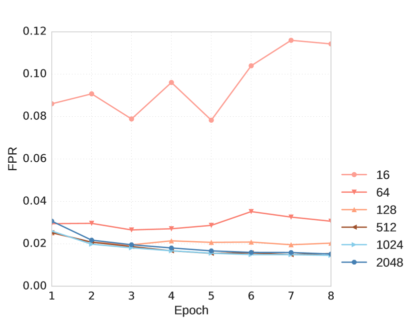
We study the influence of mini-batch size on the final descriptor performance. It is known that small mini-batches are beneficial to faster convergence and better generalization [34], while large batches allow better GPU utilization. Our loss function design should benefit from seeing more hard negative patches to learn to distinguish them from true positive patches. We report the results for batch sizes 16, 64, 128, 512, 1024, 2048. We trained the model described in Section 3.2 using Liberty sequence of Brown dataset. Results are shown in Figure 4. As expected, model performance improves with increasing the mini-batch size, as more examples are seen to get harder negatives. Although, increasing batch size to more than 512 does not bring significant benefit.

4 Empirical evaluation

Recently, Balntas et al. [23] showed that good performance on patch verification task on Brown dataset does not always mean good performance in the nearest neighbor setup and vice versa. Therefore, we have extensively evaluated learned descriptors on real-world tasks like two view matching and image retrieval.

We have selected RootSIFT [10], PCW [33], TFeat-M* [23], and L2Net [24] for direct comparison with our descriptor, as they show the best results on a variety of datasets.

4.1 Patch descriptor evaluation

Figure 5: Left to right: Verification, matching and retrieval results on HPatches dataset. All the descriptors are trained on Liberty subset of Brown [3] dataset, or are handcrafted. Comparison of descriptors trained on other datasets are in Figure 6. Marker color indicates the level of geometrical noise in: Easy, Hard and Tough. Marker type indicates the experimental setup. DiffSeq and SameSeq shows the source of negative examples for the verification task. Viewpt and Illum indicate the type of sequences for matching. None of the descriptors is trained on HPatches. The HardNet and HardNet+ were trained after NIPS with optimized hyperparameters learning rate.

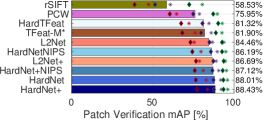
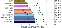
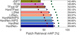
HPatches [18] is a recent dataset for local patch descriptor evaluation. It consists of 116 sequences of 6 images. The dataset is split into two parts: viewpoint – 59 sequences with significant viewpoint change and illumination – 57 sequences with significant illumination change, both natural and artificial. Keypoints are detected by DoG, Hessian and Harris detectors in the reference image and reprojected to the rest of the images in each sequence with 3 levels of geometric noise: Easy, Hard, and Tough variants. The HPatches benchmark defines three tasks: patch correspondence verification, image matching and small-scale patch retrieval. We refer the reader to the HPatches paper [18] for a detailed protocol for each task.

Results are shown in Figure 5. L2Net and HardNet have shown similar performance on the patch verification task with a small advantage of HardNet. On the matching task, even the non-augmented version of HardNet outperforms the augmented version of L2Net+ by a noticeable margin. The difference is larger in the Tough and Hard setups. Illumination sequences are more challenging than the geometric ones, for all the descriptors. We have trained network with TFeat architecture, but with proposed loss function – it is denoted as HardTFeat. It outperforms original version in matching and retrieval, while being on par with it on patch verification task.

In patch retrieval, relative performance of the descriptors is similar to the matching problem: HardNet beats L2Net+. Both descriptors significantly outperform the previous state-of-the-art, showing the superiority of the selected deep CNN architecture over the shallow TFeat model.

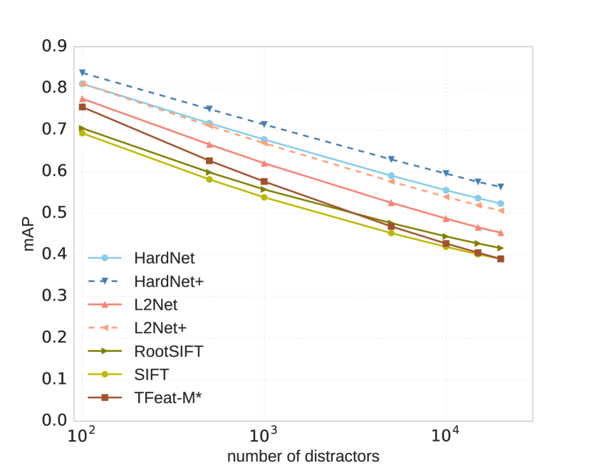
We also ran another patch retrieval experiment, varying the number of distractors (non-matching patches) in the retrieval dataset. The results are shown in Figure 4. TFeat descriptor performance, which is comparable to L2Net in the presence of low number distractors, degrades quickly as the size of the the database grows. At about 10,000 its performance drops below SIFT. This experiment explains why TFeat performs relatively poorly on the Oxford5k [35] and Paris6k [36] benchmarks, which contain around 12M and 15M distractors, respectively, see Section 4.4 for more details. Performance of the HardNet decreases slightly for both augmented and plain version and the difference in mAP to other descriptors grows with the increasing complexity of the task.

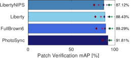
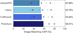
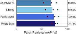
Post-NIPS update. We have studied impact of training dataset on descriptor performance. In particular, we compared commonly used Liberty subset with patches extracted by DoG detector, full Brown dataset – subsets Liberty, Notredame and Yosemite with patches, extracted by DoG and Harris detectors. We also included results by Mitra et al., who trained HardNet on new large scale PhotoSync dataset. Results are shown in Figure 6.

Figure 6: Comparison of HardNet versions, trained on different datasets. LibertyNIPS, Liberty – Liberty[3], FullBrown6 – all six subsets of Brown dataset [3], PhotoSync – new dataset from Mitra et al. [37]. Left to right: Verification, matching and retrieval results on HPatches dataset. Marker color indicates the level of geometrical noise in: Easy, Hard and Tough. Marker type indicates the experimental setup. DiffSeq and SameSeq shows the source of negative examples for the verification task. Viewpt and Illum indicate the type of sequences for matching.                                                                                                                                     None of the descriptors above was trained on HPatches. HardNet++ results are not presented since it was trained on HPatches.

4.2 Ablation study

Table 2: Comparison of the loss functions and sampling strategies on the HPatches matching task, the mean mAP is reported. CPR stands for the regularization penalty of the correlation between descriptor channels, as proposed in [24]. Hard negative mining is performed once per epoch. Best results are in bold. HardNet uses the hardest-in-batch sampling and the triplet margin loss.

Sampling / Loss	Softmin	Triplet margin	Contrastive
		$m=1$	$m=1$	$m=2$
Random	overfit
Hard negative mining	overfit
Random + CPR	0.349	0.286	0.007	0.083
Hard negative mining + CPR	0.391	0.346	0.055	0.279
Hardest in batch (ours)	0.474	0.482	0.444	0.482

For better understanding of the significance of the sampling strategy and the loss function, we conduct experiments summarized in Table 2. We train our HardNet model (architecture is exactly the same as L2Net model), change one parameter at a time and evaluate its impact.

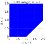
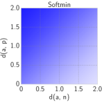
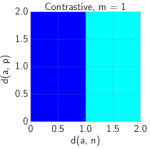
The following sampling strategies are compared: random, the proposed “hardest-in-batch”, and the “classical” hard negative mining, i.e. selecting in each epoch the closest negatives from the full training set. The following loss functions are tested: softmin on distances, triplet margin with margin $m=1$, contrastive with margins $m=1,m=2$. The last is the maximum possible distance for unit-normed descriptors. Mean mAP on HPatches Matching task is shown in Table 2.

The proposed “hardest-in-batch” clearly outperforms all the other sampling strategies for all loss functions and it is the main reason for HardNet good performance. The random sampling and “classical” hard negative mining led to huge overfit, when training loss was high, but test performance was low and varied several times from run to run. This behavior was observed with all loss function. Similar results for random sampling were reported in [24].

$\frac{\partial L}{\partial n}=\frac{\partial L}{\partial p}=1$ $\frac{\partial L}{\partial n}=0,\frac{\partial L}{\partial p}=1$ $\frac{\partial L}{\partial n}=\frac{\partial L}{\partial p}=0$

Figure 7: Contribution to the gradient magnitude from the positive and negative examples. Horizontal and vertical axes show the distance from the anchor (a) to the negative (n) and positive (p) examples respectively. Softmin loss gradient quickly decreases when $d(a,n)>d(a,p)$, unlike the triplet margin loss. For the contrastive loss, negative examples with $d(a,n)>m$ contribute zero to the gradient. The triplet margin loss and the contrastive loss with a big margin behave very similarly.

The poor results of hard negative mining (“hardest-in-the-training-set”) are surprising. We guess that this is due to dataset label noise, the mined “hard negatives” are actually positives. Visual inspection confirms this. We were able to get reasonable results with random and hard negative mining sampling only with additional correlation penalty on descriptor channels (CPR), as proposed in [24].

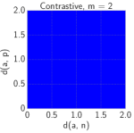
Regarding the loss functions, softmin gave the most stable results across all sampling strategies, but it is marginally outperformed by contrastive and triplet margin loss for our strategy. One possible explanation is that the triplet margin loss and contrastive loss with a large margin have constant non-zero derivative w.r.t to both positive and negative samples, see Figure 7. In the case of contrastive loss with a small margin, many negative examples are not used in the optimization (zero derivatives), while the softmin derivatives become small, once the distance to the positive example is smaller than to the negative one.

4.3 Wide baseline stereo

Figure 8: Descriptor evaluation on the W1BS patch dataset, mean area under precision-recall curve is reported. Letters denote nuisance factor, A: appearance; G: viewpoint/geometry; L: illumination; S: sensor; map2photo: satellite photo vs. map.

To validate descriptor generalization and their ability to operate in extreme conditions, we tested them on the W1BS dataset [4]. It consists of 40 image pairs with one particular extreme change between the images:

• Appearance (A): difference in appearance due to seasonal or weather change, occlusions, etc;

• Geometry (G): difference in scale, camera and object position;

• Illumination (L): significant difference in intensity, wavelength of light source;

• Sensor (S): difference in sensor data (IR, MRI).

Moreover, local features in W1BS dataset are detected with MSER [38], Hessian-Affine [11] (in implementation from [39]) and FOCI [40] detectors. They fire on different local structures than DoG. Note that DoG patches were used for the training of the descriptors. Another significant difference to the HPatches setup is the absence of the geometrical noise: all patches are perfectly reprojected to the target image in pair. The testing protocol is the same as for the HPatches matching task.

Results are shown in Figure 8. HardNet and L2Net perform comparably, former is performing better on images with geometrical and appearance changes, while latter works a bit better in map2photo and visible-vs-infrared pairs. Both outperform SIFT, but only by a small margin. However, considering the significant amount of the domain shift, descriptors perform very well, while TFeat loses badly to SIFT. HardTFeat significantly outperforms the original TFeat descriptor on the W1BS dataset, showing the superiority of the proposed loss.

Good performance on patch matching and verification task does not automatically lead to the better performance in practice, e.g. to more images registered. Therefore we also compared descriptor on wide baseline stereo setup with two metric: number of successfully matched image pairs and average number of inliers per matched pair, following the matcher comparison protocol from [4]. The only change to the original protocol is that first fast matching steps with ORB detector and descriptor were removed, as we are comparing “SIFT-replacement” descriptors.

The results are shown in Table 3. Results on Edge Foci (EF) [40], Extreme view [41] and Oxford Affine [11] datasets are saturated and all the descriptors are good enough for matching all image pairs. HardNet has an a slight advantage in a number of inliers per image. The rest of datasets: SymB [42], GDB [43], WxBS [4] and LTLL [44] have one thing in common: image pairs are or from different domain than photo (e.g. drawing to drawing) or cross-domain (e.g., drawing to photo). Here HardNet outperforms learned descriptors and is on-par with hand-crafted RootSIFT. We would like to note that HardNet was not learned to match in different domain, nor cross-domain scenario, therefore such results show the generalization ability.

Table 3: Comparison of the descriptors on wide baseline stereo within MODS matcher[4] on wide baseline stereo datasets. Number of matched image pairs and average number of inliers are reported. Numbers is the header corresponds to the number of image pairs in dataset.

	EF		EVD		OxAff		SymB		GDB		WxBS		LTLL
Descriptor	33	inl.	15	inl.	40	inl.	46	inl.	22	inl.	37	inl.	172	inl.
RootSIFT	33	32	15	34	40	169	45	43	21	52	11	93	123	27
TFeat-M*	32	30	15	37	40	265	40	45	16	72	10	62	96	29
L2Net+	33	34	15	34	40	304	43	46	19	78	9	51	127	26
HardNet+	33	35	15	41	40	316	44	47	21	75	11	54	127	31

4.4 Image retrieval

Table 4: Performance (mAP) evaluation on bag-of-words (BoW) image retrieval. Vocabulary consisting of 1M visual words is learned on independent dataset, that is, when evaluating on Oxford5k, the vocabulary is learned with features of Paris6k and vice versa. SV: spatial verification. QE: query expansion. The best results are highlighted in bold. All the descriptors except SIFT and HardNet++ were learned on Liberty sequence of Brown dataset [3]. HardNet++ is trained on union of Brown and HPatches [18] datasets.

	Oxford5k			Paris6k
Descriptor	BoW	BoW+SV	BoW+QE	BoW	BoW+SV	BoW+QE
TFeat-M* [23]	46.7	55.6	72.2	43.8	51.8	65.3
RootSIFT [10]	55.1	63.0	78.4	59.3	63.7	76.4
L2Net+ [24]	59.8	67.7	80.4	63.0	66.6	77.2
HardNet	59.0	67.6	83.2	61.4	67.4	77.5
HardNet+	59.8	68.8	83.0	61.0	67.0	77.5
HardNet++	60.8	69.6	84.5	65.0	70.3	79.1

We evaluate our method, and compare against the related ones, on the practical application of image retrieval with local features. Standard image retrieval datasets are used for the evaluation, i.e., Oxford5k [35] and Paris6k [36] datasets. Both datasets contain a set of images (5062 for Oxford5k and 6300 for Paris6k) depicting 11 different landmarks together with distractors. For each of the 11 landmarks there are 5 different query regions defined by a bounding box, constituting 55 query regions per dataset. The performance is reported as mean average precision (mAP) [35].

In the first experiment, for each image in the dataset, multi-scale Hessian-affine features [32] are extracted. Exactly the same features are described by ours and all related methods, each of them producing a 128-D descriptor per feature. Then, k-means with approximate nearest neighbor [21] is used to learn a 1 million visual vocabulary on an independent dataset, that is, when evaluating on Oxford5k, the vocabulary is learned with descriptors of Paris6k and vice versa. All descriptors of testing dataset are assigned to the corresponding vocabulary, so finally, an image is represented by the histogram of visual word occurrences, i.e., the bag-of-words (BoW) [1] representation, and an inverted file is used for an efficient search. Additionally, spatial verification (SV) [35], and standard query expansion (QE) [36] are used to re-rank and refine the search results. Comparison with the related work on patch description is presented in Table 4. HardNet+ and L2Net+ perform comparably across both datasets and all settings, with slightly better performance of HardNet+ on average across all results (average mAP 69.5 vs. 69.1). RootSIFT, which was the best performing descriptor in image retrieval for a long time, falls behind with average mAP 66.0 across all results.

We also trained HardNet++ version – with all available training data at the moment: union of Brown and HPatches datasets, instead of just Liberty sequence from Brown for the HardNet+. It shows the benefits of having more training data and is performing best for all setups.

Finally, we compare our descriptor with the state-of-the-art image retrieval approaches that use local features. For fairness, all methods presented in Table 5 use the same local feature detector as described before, learn the vocabulary on an independent dataset, and use spatial verification (SV) and query expansion (QE). In our case (HardNet++–HQE), a visual vocabulary of 65k visual words is learned, with additional Hamming embedding (HE) [45] technique that further refines descriptor assignments with a 128 bits binary signature. We follow the same procedure as RootSIFT–HQE [46] method, by replacing RootSIFT with our learned HardNet++ descriptor. Specifically, we use: (i) weighting of the votes as a decreasing function of the Hamming distance [47]; (ii) burstiness suppression [47]; (iii) multiple assignments of features to visual words [36, 48]; and (iv) QE with feature aggregation [46]. All parameters are set as in [46]. The performance of our method is the best reported on both Oxford5k and Paris6k when learning the vocabulary on an independent dataset (mAP 89.1 was reported [10] on Oxford5k by learning it on the same dataset comprising the relevant images), and using the same amount of features (mAP 89.4 was reported [46] on Oxford5k when using twice as many local features, i.e., 22M compared to 12.5M used here).

Table 5: Performance (mAP) comparison with the state-of-the-art image retrieval with local features. Vocabulary is learned on independent dataset, that is, when evaluating on Oxford5k, the vocabulary is learned with features of Paris6k and vice versa. All presented results are with spatial verification and query expansion. VS: vocabulary size. SA: single assignment. MA: multiple assignments. The best results are highlighted in bold.

		Oxford5k		Paris6k
Method	VS	SA	MA	SA	MA
SIFT–BoW [39]	1M	78.4	82.2	–	–
SIFT–BoW-fVocab [49]	16M	74.0	84.9	73.6	82.4
RootSIFT–HQE [46]	65k	85.3	88.0	81.3	82.8
HardNet++–HQE	65k	86.8	88.3	82.8	84.9

5 Conclusions

We proposed a novel loss function for learning a local image descriptor that relies on the hard negative mining within a mini-batch and the maximization of the distance between the closest positive and closest negative patches. The proposed sampling strategy outperforms classical hard-negative mining and random sampling for softmin, triplet margin and contrastive losses.

The resulting descriptor is compact – it has the same dimensionality as SIFT (128), it shows state-of-art performance on standard matching, patch verification and retrieval benchmarks and it is fast to compute on a GPU. The training source code and the trained convnets are available at https://github.com/DagnyT/hardnet.

References

- Sivic and Zisserman [2003] Josef Sivic and Andrew Zisserman. Video google: A text retrieval approach to object matching in videos. In International Conference on Computer Vision (ICCV), pages 1470–1477, 2003.
- Radenovic et al. [2016] Filip Radenovic, Giorgos Tolias, and Ondrej Chum. CNN image retrieval learns from BoW: Unsupervised fine-tuning with hard examples. In European Conference on Computer Vision (ECCV), pages 3–20, 2016.
- Brown and Lowe [2007] Matthew Brown and David G. Lowe. Automatic panoramic image stitching using invariant features. International Journal of Computer Vision (IJCV), 74(1):59–73, 2007.
- Mishkin et al. [2015a] Dmytro Mishkin, Jiri Matas, Michal Perdoch, and Karel Lenc. Wxbs: Wide baseline stereo generalizations. Arxiv 1504.06603, 2015a.
- Schonberger et al. [2015] Johannes L. Schonberger, Filip Radenovic, Ondrej Chum, and Jan-Michael Frahm. From single image query to detailed 3D reconstruction. In Conference on Computer Vision and Pattern Recognition (CVPR), pages 5126–5134, 2015.
- Schonberger and Frahm [2016] Johannes L. Schonberger and Jan-Michael Frahm. Structure-from-motion revisited. In Conference on Computer Vision and Pattern Recognition (CVPR), pages 4104–4113, 2016.
- Choy et al. [2016] Christopher B. Choy, JunYoung Gwak, Silvio Savarese, and Manmohan Chandraker. Universal correspondence network. In Advances in Neural Information Processing Systems, pages 2414–2422, 2016.
- Kendall et al. [2015] Alex Kendall, Matthew Grimes, and Roberto Cipolla. Posenet: A convolutional network for real-time 6-DOF camera relocalization. In International Conference on Computer Vision (ICCV), 2015.
- Lowe [2004] David G. Lowe. Distinctive image features from scale-invariant keypoints. International Journal of Computer Vision (IJCV), 60(2):91–110, 2004.
- Arandjelovic and Zisserman [2012] Relja Arandjelovic and Andrew Zisserman. Three things everyone should know to improve object retrieval. In Conference on Computer Vision and Pattern Recognition (CVPR), pages 2911–2918, 2012.
- Mikolajczyk and Schmid [2004] Krystian Mikolajczyk and Cordelia Schmid. Scale & affine invariant interest point detectors. International Journal of Computer Vision (IJCV), 60(1):63–86, 2004.
- Rublee et al. [2011] Ethan Rublee, Vincent Rabaud, Kurt Konolige, and Gary Bradski. ORB: An efficient alternative to SIFT or SURF. In International Conference on Computer Vision (ICCV), pages 2564–2571, 2011.
- Yi et al. [2016] Kwang Moo Yi, Eduard Trulls, Vincent Lepetit, and Pascal Fua. LIFT: Learned invariant feature transform. In European Conference on Computer Vision (ECCV), pages 467–483, 2016.
- Han et al. [2015] Xufeng Han, T. Leung, Y. Jia, R. Sukthankar, and A. C. Berg. Matchnet: Unifying feature and metric learning for patch-based matching. In Conference on Computer Vision and Pattern Recognition (CVPR), pages 3279–3286, 2015.
- Zagoruyko and Komodakis [2015] Sergey Zagoruyko and Nikos Komodakis. Learning to compare image patches via convolutional neural networks. In Conference on Computer Vision and Pattern Recognition (CVPR), 2015.
- Bursuc et al. [2015] Andrei Bursuc, Giorgos Tolias, and Herve Jegou. Kernel local descriptors with implicit rotation matching. In ACM International Conference on Multimedia Retrieval, 2015.
- Dong and Soatto [2015] Jingming Dong and Stefano Soatto. Domain-size pooling in local descriptors: DSP-SIFT. In Conference on Computer Vision and Pattern Recognition (CVPR), pages 5097–5106, 2015.
- Balntas et al. [2017] Vassileios Balntas, Karel Lenc, Andrea Vedaldi, and Krystian Mikolajczyk. HPatches: A benchmark and evaluation of handcrafted and learned local descriptors. In Conference on Computer Vision and Pattern Recognition (CVPR), 2017.
- Schonberger et al. [2017] Johannes L. Schonberger, Hans Hardmeier, Torsten Sattler, and Marc Pollefeys. Comparative evaluation of hand-crafted and learned local features. In Conference on Computer Vision and Pattern Recognition (CVPR), 2017.
- Simonyan et al. [2012] Karen Simonyan, Andrea Vedaldi, and Andrew Zisserman. Descriptor learning using convex optimisation. In European Conference on Computer Vision (ECCV), pages 243–256, 2012.
- Muja and Lowe [2009] Marius Muja and David G. Lowe. Fast approximate nearest neighbors with automatic algorithm configuration. In International Conference on Computer Vision Theory and Application (VISSAPP), pages 331–340, 2009.
- Simo-Serra et al. [2015] Edgar Simo-Serra, Eduard Trulls, Luis Ferraz, Iasonas Kokkinos, Pascal Fua, and Francesc Moreno-Noguer. Discriminative learning of deep convolutional feature point descriptors. In International Conference on Computer Vision (ICCV), pages 118–126, 2015.
- Balntas et al. [2016] Vassileios Balntas, Edgar Riba, Daniel Ponsa, and Krystian Mikolajczyk. Learning local feature descriptors with triplets and shallow convolutional neural networks. In British Machine Vision Conference (BMVC), 2016.
- Yurun Tian and Wu [2017] Bin Fan Yurun Tian and Fuchao Wu. L2-Net: Deep learning of discriminative patch descriptor in euclidean space. In Conference on Computer Vision and Pattern Recognition (CVPR), 2017.
- Lee et al. [2015] Chen-Yu Lee, Saining Xie, Patrick Gallagher, Zhengyou Zhang, and Zhuowen Tu. Deeply-supervised nets. In Artificial Intelligence and Statistics, pages 562–570, 2015.
- Ioffe and Szegedy [2015] Sergey Ioffe and Christian Szegedy. Batch Normalization: Accelerating Deep Network Training by Reducing Internal Covariate Shift. ArXiv 1502.03167, 2015.
- Nair and Hinton [2010] Vinod Nair and Geoffrey E. Hinton. Rectified linear units improve restricted boltzmann machines. In International Conference on Machine Learning (ICML), pages 807–814, 2010.
- Srivastava et al. [2014] Nitish Srivastava, Geoffrey E Hinton, Alex Krizhevsky, Ilya Sutskever, and Ruslan Salakhutdinov. Dropout: a simple way to prevent neural networks from overfitting. Journal of Machine Learning Research (JMLR), 15(1):1929–1958, 2014.
- Saxe et al. [2014] Andrew M. Saxe, James L. McClelland, and Surya Ganguli. Exact solutions to the nonlinear dynamics of learning in deep linear neural networks. In Proceedings of ICLR, 2014. URL http://arxiv.org/abs/1312.6120.
- [30] PyTorch. http://pytorch.org.
- Kumar B. G. et al. [2016] Vijay Kumar B. G., Gustavo Carneiro, and Ian Reid. Learning local image descriptors with deep siamese and triplet convolutional networks by minimising global loss functions. In Conference on Computer Vision and Pattern Recognition (CVPR), pages 5385–5394, 2016.
- Mikolajczyk et al. [2005] Krystian Mikolajczyk, Tinne Tuytelaars, Cordelia Schmid, Andrew Zisserman, Jiri Matas, Frederik Schaffalitzky, Timor Kadir, and Luc Van Gool. A comparison of affine region detectors. International Journal of Computer Vision (IJCV), 65(1):43–72, 2005.
- Mukundan et al. [2017] Arun Mukundan, Giorgos Tolias, and Ondrej Chum. Multiple-kernel local-patch descriptor. In British Machine Vision Conference, 2017. URL https://arxiv.org/pdf/1707.07825.pdf.
- Wilson and Martinez [2003] D. Randall Wilson and Tony R. Martinez. The general inefficiency of batch training for gradient descent learning. Neural Networks, 16(10):1429–1451, 2003.
- Philbin et al. [2007] James Philbin, Ondrej Chum, Michael Isard, Josef Sivic, and Andrew Zisserman. Object retrieval with large vocabularies and fast spatial matching. In Conference on Computer Vision and Pattern Recognition (CVPR), pages 1–8, 2007.
- Philbin et al. [2008] James Philbin, Ondrej Chum, Michael Isard, Josef Sivic, and Andrew Zisserman. Lost in quantization: Improving particular object retrieval in large scale image databases. In Conference on Computer Vision and Pattern Recognition (CVPR), pages 1–8, 2008.
- Mitra et al. [2018] R. Mitra, N. Doiphode, U. Gautam, S. Narayan, S. Ahmed, S. Chandran, and A. Jain. A Large Dataset for Improving Patch Matching. ArXiv e-prints, January 2018.
- Matas et al. [2002] Jiri Matas, Ondrej Chum, Martin Urban, and Tomas Pajdla. Robust wide baseline stereo from maximally stable extrema regions. In British Machine Vision Conference (BMVC), pages 384–393, 2002.
- Perdoch et al. [2009] Michal Perdoch, Ondrej Chum, and Jiri Matas. Efficient representation of local geometry for large scale object retrieval. In Conference on Computer Vision and Pattern Recognition (CVPR), pages 9–16, 2009.
- Zitnick and Ramnath [2011] C. Lawrence Zitnick and Krishnan Ramnath. Edge foci interest points. In International Conference on Computer Vision (ICCV), pages 359–366, 2011.
- Mishkin et al. [2015b] Dmytro Mishkin, Jiri Matas, and Michal Perdoch. Mods: Fast and robust method for two-view matching. Computer Vision and Image Understanding, 141:81 – 93, 2015b. doi: https://doi.org/10.1016/j.cviu.2015.08.005.
- Hauagge and Snavely [2012] Daniel C. Hauagge and Noah Snavely. Image matching using local symmetry features. In Computer Vision and Pattern Recognition (CVPR), pages 206–213, 2012.
- Yang et al. [2007] Gehua Yang, Charles V Stewart, Michal Sofka, and Chia-Ling Tsai. Registration of challenging image pairs: Initialization, estimation, and decision. Pattern Analysis and Machine Intelligence (PAMI), 29(11):1973–1989, 2007.
- Fernando et al. [2015] Basura Fernando, Tatiana Tommasi, and Tinne Tuytelaars. Location recognition over large time lags. Computer Vision and Image Understanding, 139:21 – 28, 2015. ISSN 1077-3142. doi: https://doi.org/10.1016/j.cviu.2015.05.016.
- Jegou et al. [2010a] Herve Jegou, Matthijs Douze, and Cordelia Schmid. Improving bag-of-features for large scale image search. International Journal of Computer Vision (IJCV), 87(3):316–336, 2010a.
- Tolias and Jegou [2014] Giorgos Tolias and Herve Jegou. Visual query expansion with or without geometry: refining local descriptors by feature aggregation. Pattern Recognition, 47(10):3466–3476, 2014.
- Jegou et al. [2009] Herve Jegou, Matthijs Douze, and Cordelia Schmid. On the burstiness of visual elements. In Computer Vision and Pattern Recognition (CVPR), pages 1169–1176, 2009.
- Jegou et al. [2010b] Herve Jegou, Cordelia Schmid, Hedi Harzallah, and Jakob Verbeek. Accurate image search using the contextual dissimilarity measure. Pattern Analysis and Machine Intelligence (PAMI), 32(1):2–11, 2010b.
- Mikulik et al. [2013] Andrej Mikulik, Michal Perdoch, Ondřej Chum, and Jiří Matas. Learning vocabularies over a fine quantization. International Journal of Computer Vision (IJCV), 103(1):163–175, 2013.