Next generation extended Lagrangian first principles molecular dynamics

Abstract

Extended Lagrangian Born-Oppenheimer molecular dynamics [Phys. Rev. Lett., ${\bf 100}$, 123004 (2008)] is formulated for general Hohenberg-Kohn density functional theory and compared to the extended Lagrangian framework of first principles molecular dynamics by Car and Parrinello [Phys. Rev. Lett. ${\bf 55}$, 2471 (1985)]. It is shown how extended Lagrangian Born-Oppenheimer molecular dynamics overcomes several shortcomings of regular, direct Born-Oppenheimer molecular dynamics, while improving or maintaining important features of Car-Parrinello simulations. The accuracy of the electronic degrees of freedom in extended Lagrangian Born-Oppenheimer molecular dynamics, with respect to the exact Born-Oppenheimer solution, is of second order in the size of the integration time step and of fourth order in the potential energy surface. Improved stability over recent formulations of extended Lagrangian Born-Oppenheimer molecular dynamics is achieved by generalizing the theory to finite temperature ensembles, using fractional occupation numbers in the calculation of the inner-product kernel of the extended harmonic oscillator that appears as a preconditioner in the electronic equations of motion. Materials systems that normally exhibit slow self-consistent field convergence can be simulated using integration time steps of the same order as in direct Born-Oppenheimer molecular dynamics, but without the requirement of an iterative, non-linear electronic ground state optimization prior to the force evaluations and without a systematic drift in the total energy. In combination with proposed low-rank and on-the-fly updates of the kernel, this formulation provides an efficient and general framework for quantum based Born-Oppenheimer molecular dynamics simulations.

I Introduction

Quantum based molecular dynamics, using classical molecular trajectories, but with the interatomic forces calculated on-the-fly from a quantum mechanical description of the underlying electronic structure, offers an almost universal simulation engine for computational materials science, chemistry and molecular biology. Similar to classical molecular dynamics Allen and Tildesley (1990); Karplus and Petsko (1990); vanGusteren and Berendsen (1990); Tuckerman and Martyna (2000); Frenkel and Smit (2002); Karplus and McCammon (2002); Sanbonmatsu and Tung (2007); Orozco (2014); Perilla et al. (2015), quantum based molecular dynamics can be used to analyze, predict and manipulate a broad range of systems and phenomena Marx and Hutter (2000); Tuckerman (2002); Kirchner et al. (2012); Hutter (2012). However, since quantum based molecular dynamics includes an explicit quantum mechanical description of the electrons, it can be used also for materials that are difficult or impossible to simulate with classical force field methods. Quantum based molecular dynamics therefore provides a more general approach that can handle phenomena such as electronic excitations in photo voltaics, quantum size effects in nanodevices, spin-polarization in magnetic materials, quantum response properties such as the conductivity or the polarizability, thermal excitations in warm dense matter, as well as bond formation and dissociation with the associated charge transfer in chemical reactions.

While some early applications of quantum based molecular dynamics simulations date back to the mid 70’s Wang and Karplus (1973); Leforestier (1978); Warshel and Karplus (1975), it was only after the introduction of the ingenious unified extended Lagrangian approach to first principles electronic structure theory by Car and Parrinello Car and Parrinello (1985); Remler and Madden (1990); Pastore et al. (1991); Bornemann and Schütte (1998); Marx and Hutter (2000); Hutter (2012) that stable and efficient molecular dynamics simulations with predictive quantum accuracy became practically feasible for a broad range of materials systems. Their pioneering contribution unraveled major developments of first principles molecular dynamics simulation tools and opened the door to a number of new applications in materials science, chemistry and molecular biology Remler and Madden (1990); Marx and Hutter (2000); Carloni et al. (2002); Tuckerman (2002); Senn and Thiel (2009); Kirchner et al. (2012); Hutter (2012). In contrast to the straightforward direct Born-Oppenheimer approach, where the interatomic forces are calculated with an optimized relaxed electronic ground state in each time step Heitler and London (1927); Born and Oppenheimer (1927); Barnett and Landman (1993); Kresse and Hafner (1993); Marx and Hutter (2000), Car-Parrinello molecular dynamics avoids the ground state relaxation. Instead, the electronic degrees of freedom are included as dynamical variables that approximately follow the electronic ground state. This formulation avoids problems arising from the non-linear iterative ground state optimization that is necessary in a direct Born-Oppenheimer simulation, such as a high computational overhead or non-conservative forces and a systematic drift in the total energy Remler and Madden (1990); Pulay and Fogarasi (2004); Niklasson et al. (2006); Kühne et al. (2007).

Extended Lagrangian Car-Parrinello molecular dynamics has been adapted to multiple research fields. For example, the plane-wave basis functions that were used to represent the electronic degrees of freedom in the original formulation, have been modified to include localized atomic-orbitals Hartke and Carter (1992), the charge density Lambert et al. (2006), or the atomic-orbital density matrix Schlegel et al. (2001); Iyengar et al. (2001); Herbert and Head-Gordon (2004). This allows Car-Parrinello molecular dynamics to be applied to a broad range of problems including, for example, warm dense matter Lambert et al. (2006), quantum chemistry simulations using correlated wavefunction methods Li et al. (2016), and to extended systems using linear scaling electronic structure theory Goedecker (1999); Bowler and Miyazaki (2012); Schlegel et al. (2001); Iyengar et al. (2001); Herbert and Head-Gordon (2004). Car-Parrinello based techniques are often referred to simply as ”the extended Lagrangian approach”. This is unfortunate, since there are a number of different extended Lagrangian approaches. Probably the first extended Lagrangian formulations in molecular dynamics were introduced to include the effects of thermostats or barostats in classical force field simulations Andersen (1980); Parrinello and Rahman (1980); Nose (1984) – and recently, a new extended Lagrangian formulation of first-principles Born-Oppenheimer molecular dynamics was proposed by the author and his co-workers in a series of papers Niklasson (2008a); Niklasson et al. (2009); Odell et al. (2009); Steneteg et al. (2010); Zheng et al. (2011); Cawkwell and Niklasson (2012); Souvatzis and Niklasson (2014); Niklasson and Cawkwell (2014); Aradi et al. (2015); Martinez et al. (2015); Vitale et al. (2017); Albaugh et al. (2017). This formulation is the main focus of this article.

The extended Lagrangian formulation of first-principles Born-Oppenheimer molecular dynamics differs from the Car-Parrinello method, although some interesting connections have been discussed Kirchner et al. (2012); Hutter (2012); Lin et al. (2014). Both methods provide general theoretical frameworks that are applicable to a broad class of materials problems and electronic structure methods. However, extended Lagrangian Born-Oppenheimer molecular dynamics is a higher-order method and it is based on a different Lagrangian that avoids the orthonormalization (or the idempotency) constraints as well as the problem of choosing material-dependent fictitious electron mass parameters.

Extended Lagrangian Born-Oppenheimer molecular dynamics Niklasson et al. (2006); Niklasson (2008a) was originally developed to overcome shortcomings of direct Born-Oppenheimer molecular dynamics, such as the irreversible and unphysical evolution of the electronic degrees of freedom, which is causing a systematic drift in the total energy and temperature Remler and Madden (1990); Pulay and Fogarasi (2004). The original idea was based on a time-reversible extrapolation of the electronic degrees of freedom from previous time steps followed by a fast, approximate update of the Born-Oppenheimer potential energy surface and the forces Niklasson et al. (2006). This ad hoc approach, which has many similarities with, for example, the Fock-dynamics scheme by Pulay and Fogarasi Pulay and Fogarasi (2004); Herbert and Head-Gordon (2005) as well as the technique by Kühne et. al Kühne et al. (2007); Kolafa (2003), was thereafter generalized and formulated in terms of an extended Lagrangian framework in the spirit of Car-Parrinello molecular dynamics Niklasson (2008a). This framework represents a new generation extended Lagrangian first principles molecular dynamics that overcomes shortcomings of direct Born-Oppenheimer molecular dynamics while maintaining important benefits of Car’s and Parrinello’s formulation.

First I present extended Lagrangian Born-Oppenheimer molecular dynamics in terms of Hohenberg-Kohn density functional theory and discuss its relation to Car-Parrinello molecular dynamics. Thereafter, I formulate a generalized extended Lagrangian Born-Oppenheimer molecular dynamics for thermal (or ensemble) Kohn-Sham density functional theory with fractional occupation numbers. I then focus on the calculation and approximation of the inner-product kernel that appears in the extended harmonic oscillator of the Lagrangian. I show how this kernel can be constructed on-the-fly through a sequence of low-rank updates. At the end I demonstrate the framework with examples using self-consistent-charge density functional based tight-binding (SCC-DFTB) theory, before I outline remaining challenges and give a summary and conclusions.

II Next generation extended Lagrangian first principles molecular dynamics

Extended Lagrangian Born-Oppenheimer molecular dynamics was first formulated in Ref. Niklasson (2008a), and then developed and adapted to a number of electronic structure codes at different levels of theory and choices of dynamical variables for the electronic degrees of freedom Niklasson et al. (2009); Odell et al. (2009); Steneteg et al. (2010); Zheng et al. (2011); Niklasson et al. (2011); Cawkwell and Niklasson (2012); Souvatzis and Niklasson (2014); Niklasson and Cawkwell (2014); Aradi et al. (2015); Arita et al. (2014); Lin et al. (2014); Nomura et al. (2015); Albaugh et al. (2015); Niklasson et al. (2016); Vitale et al. (2017); Albaugh et al. (2017). Recently the framework was introduced in a more general form, including a kernel that defines the inner product norm of the extended harmonic oscillator Niklasson and Cawkwell (2014). This kernel appears similar to a preconditioner in the equations of motion of the extended electronic degrees of freedom, which can be used to improve the stability and the accuracy of a simulation. In early formulations of extended Lagrangian Born-Oppenheimer molecular dynamics a few self-consistent field iterations were sometimes required prior to the force evaluations. With the generalized framework, which is based on an underlying shadow Hamiltonian dynamics, the self-consistent field procedure can be avoided completely. In this section I will briefly review this formulation in a more rigorous form based on Hohenberg’s and Kohn’s non-degenerate ground state density functional theory. Extensions beyond Hohenberg-Kohn density functional theory should be straightforward, e.g. within Levy’s and Lieb’s formulations Levy (1979); Lieb (1983), but this will not be discussed here. The purpose is to present a clear and fairly brief formulation of extended Lagrangian Born-Oppenheimer molecular dynamics.

II.1 Density functional theory for Born-Oppenheimer molecular dynamics

In Hohenberg’s and Kohn’s original density functional theory Hohenberg and Kohn (1964); Parr and Yang (1989); Dreizler and Gross (1990) the electronic ground state density, $\rho_{\rm min}({\bf r})$, of a non-degenerate electron system in an external potential, $v({\bf R,r})$, that moves with the nuclear coordinates, ${\bf R}=\{R_{I}\}$, is given through a constrained functional minimization over all $v$-representable densities, $\rho({\bf r})\in{\cal V}$, such that

$$\rho_{\rm min}({\bf r})=\arg\min_{\rho\in{\cal V}}\left\{F[\rho]+\int v({\bf R,r})\rho({\bf r})d{\bf r}\right\},$$ (1)

where $F[\rho]$ is a universal functional of the electron density. The Born-Oppenheimer potential energy surface is then given by

$$U_{\rm BO}({\bf R})=F[\rho_{\rm min}]+\int v({\bf R,r})\rho_{\rm min}({\bf r})d{\bf r}+V_{nn}({\bf R}),$$ (2)

including a nuclear-nuclear (or ion-ion) interaction potential, $V_{nn}({\bf R})$. A Born-Oppenheimer molecular dynamics based on density functional theory can then be defined through the Lagrangian

$${\cal L}_{\rm BO}({\bf R},{\bf{\dot{R}}})=\frac{1}{2}\sum_{I}M_{I}{\dot{R}}_{I}^{2}-U_{\rm BO}({\bf R}),$$ (3)

where $M_{I}$ are the nuclear masses and the dots denote time derivatives. The Euler-Lagrange’s equations,

$$\frac{d}{dt}\left(\frac{\partial{\cal L}_{\rm BO}}{\partial{\dot{R}}_{I}}\right)=\frac{\partial{\cal L}_{\rm BO}}{\partial{R}_{I}},$$ (4)

then gives us the equations of motion,

$$M_{I}{\ddot{R}_{I}}=-\frac{\partial U_{\rm BO}({\bf R})}{\partial R_{I}}.$$ (5)

The corresponding constant of motion is the Born-Oppenheimer Hamiltonian

$${\cal H}_{\rm BO}=\frac{1}{2}\sum_{I}M_{I}{\dot{R}}_{I}^{2}+U_{\rm BO}({\bf R}).$$ (6)

II.2 Shadow Born-Oppenheimer potential energy surface

The main cost associated with density functional based Born-Oppenheimer molecular dynamics is the non-linear ground state minimization in Eq. (1), which is required prior to each force evaluation in Eq. (5). The ground state optimization is typically given through an iterative self-consistent-field optimization procedure Broyden (1965); Anderson (1965); Pulay (1980); Srivastava (1984); Kerker (1981); Johnson (1988) or with a constrained direct energy functional minimization using, for example, a non-linear conjugate gradient method Fletcher (1970); Stich et al. (1989); Hutter et al. (1994); Weber et al. (2008). In practice these techniques are always approximate and incomplete. This incompleteness, combined with initial guesses to the optimization that are extrapolated from previous time steps, which is used to reduce the computational overhead, leads to errors in the forces and a systematic drift in the total energy or an unphysical statistical temperature distribution in canonical simulations Remler and Madden (1990); Pulay and Fogarasi (2004); Martinez et al. (2015). These problems all arise from the non-linearity of the universal density functional $F[\rho]$. To avoid the expensive, yet still approximate, iterative ground state optimization, we can replace the universal functional $F[\rho]$ with an approximate expression $F^{(1)}[\rho,n]$, given from a linearization of $F[\rho]$ around some approximate, constant ground state density $n({\bf r})$, i.e. where

$$F[\rho]\approx F^{(1)}[\rho,n]=F[n]+\int\left.\frac{\delta F[\rho]}{\delta\rho({\bf r})}\right|_{\rho=n}\left(\rho({\bf r})-n({\bf r})\right)d{\bf r}.$$ (7)

This gives us the corresponding $n$-dependent linearized density functional,

$$E^{(1)}[\rho,n]=F^{(1)}[\rho,n]+\int v({\bf R},{\bf r})\rho({\bf r})d{\bf r}.$$ (8)

We now approximate the exact ground state density, $\rho_{\rm min}({\bf r})$, by the constrained minimization

$$\rho^{(1)}[n]({\bf r})=\arg\min_{\rho\in{\cal V}}\left\{F^{(1)}[\rho,n]+\int v({\bf R,r})\rho({\bf r})d{\bf r}\right\},$$ (9)

or more generally by a variationally stationary solution, $\rho^{(1)}_{\rm min}[n]({\bf r})$, of the linearized functional with respect to the constrained density $\rho({\bf r})\in{\cal V}$, i.e. by solving

$$\left.\frac{\delta E^{(1)}[\rho,n]}{\delta\rho}\right|_{\rho\in{\cal V}}=0.$$ (10)

The approximate, but still variationally optimized, ground state density $\rho^{(1)}_{\rm min}[n]({\bf r})$ defines the $n$-dependent, approximate Born-Oppenheimer potential energy surface,

$$U^{(1)}_{\rm BO}[n]({\bf R})=F^{(1)}[\rho^{(1)}_{\rm min},n]+\int v({\bf R},{\bf r})\rho^{(1)}_{\rm min}({\bf r})d{\bf r}+V_{nn}({\bf R}).$$ (11)

Since the solution of Eq. (10) is given for a linearized functional, the iterative self-consistent-field optimization procedure is avoided and the $n$-dependent ground state density, $\rho_{\rm min}^{(1)}[n]({\bf r})$, can be calculated directly in a single optimization step at only a fraction of the cost of the original problem.

The idea is to use $U^{(1)}_{\rm BO}[n]({\bf R})$ as an approximate shadow potential from which exact forces can be calculated with a low computational cost. Such a backward analysis approach is frequently used in classical molecular dynamics. Instead of calculating approximate forces for an underlying exact Hamiltonian, exact forces are calculated for an approximate shadow Hamiltonian that closely follows the exact Hamiltonian. A large class of symplectic or geometric integration schemes can be constructed in this way, e.g. the well-known velocity Verlet or leap-frog scheme Channel and Scovel (1990); McLachlan and Atela (1992); Leimkuhler and Reich (2004); Engel et al. (2005). As I will describe below, the approximate Born-Oppenheimer potential energy surface, $U^{(1)}_{\rm BO}[n]({\bf R})$, makes this shadow Hamiltonian approach possible also for non-linear self-consistent-field theory. However, the general application of this technique has some limitations. In particular, the conditions under which the construction of $U^{(1)}_{\rm BO}[n]({\bf R})$, Eqs. (7)-(11), works as an accurate approximation of the exact ground state potential, $U_{\rm BO}({\bf R})$ in Eq. (2), are not well understood for general Hohenberg-Kohn theory and some caution is therefore necessary. In fact, it is straightforward to chose hypothetical functional expressions and constraints under which a construction like the one in Eqs. (7)-(11) both works and fails as an accurate approximation. Here we have to assume that the right (although unknown) conditions are met and that the construction gives an approximation where $U^{(1)}_{\rm BO}[n]({\bf R})\approx U_{\rm BO}({\bf R})$, with the size of the (unsigned) energy difference between $U^{(1)}_{\rm BO}[n]({\bf R})$ and the exact Born-Oppenheimer surface $U_{\rm BO}({\bf R})$ scaling as $\Delta\rho^{2}$, where $\Delta\rho$ is the size in the difference $(\rho_{\rm min}-n)$ or the residual $(\rho_{\rm min}^{(1)}[n]-n)$. We further assume that

$$\partial U^{(1)}_{\rm BO}[n]({\bf R})/\partial n\sim\rho_{\rm min}^{(1)}[n]-n.$$ (12)

So far, the motivations for these assumptions are given mainly by model examples and a posteriori numerical analysis. However, in Kohn-Sham density functional theory, $U^{(1)}_{\rm BO}[n]({\bf R})$ is directly related to the Harris-Foulkes functional Harris (1985); Foulkes and Haydock (1989), which has the desired properties, and in the related Hartree-Fock theory the corresponding assumptions (with the density replaced by a density matrix) also hold. For general Hohenberg-Kohn density functional theory, any formal proof of the validity and accuracy of the approximation based on the variationally optimized constrained solution using the linearized universal functional approximation is left for the future.

The approximation of $U_{\rm BO}({\bf R})$ presented above is not the only option. Other approaches following the same basic idea that provides a simplified shadow potential energy surface for non-linear self-consistent field theory are also possible. This is of particular interest to methods that are different from Kohn-Sham implementations of density functional theory, e.g. orbtial-free Thomas-Fermi density functional theory, excited state dynamics, methods for strongly correlated electrons, and extensions to polarizable force field methods Albaugh et al. (2015); Vitale et al. (2017); Albaugh et al. (2017). Shadow potential methods for non-linear self-consistent field theory represents an interesting and potentially fruitful area of research.

II.3 Extended Lagrangian

A straightforward application of the shadow potential energy surface $U^{(1)}_{\rm BO}[n]({\bf R})$ in the molecular dynamics scheme in Eq. (3) would not work. As the molecular trajectories evolve, the accuracy of the linearized expression around a constant density $n({\bf r})$ would become progressively worse and if we update $n({\bf r})$ as a function of the nuclear positions ${\bf R}$ we would get additional force terms depending on $\partial n/\partial R_{I}$ that are difficult to calculate. A solution to these problems is given by including $n({\bf r})$ as a dynamical variable field, which follows the ground state density through a harmonic oscillator. We can do this with the extended Lagrangian,

$$\begin{array}[]{l}{\displaystyle{\cal L}_{\rm XBO}({\bf R},{\bf{\dot{R}}},n,{\dot{n}})=\frac{1}{2}\sum_{I}M_{I}{\dot{R}_{I}}^{2}-U^{(1)}_{\rm BO}[n]({\bf R})}\\ {}{}\\ {\displaystyle~{}~{}+\frac{\mu}{2}\int({\dot{n}}({\bf r}))^{2}d{\bf r}}\\ {}{}\\ {\displaystyle~{}~{}~{}~{}-\frac{\mu\omega^{2}}{2}\iiint\left(\rho_{\rm min}^{(1)}[n]({\bf r})-n({\bf r})\right)K({\bf r^{\prime}},{\bf r})}\\ {}{}\\ {\displaystyle~{}~{}~{}~{}~{}~{}\times K({\bf r^{\prime}},{\bf r^{\prime\prime}})\left(\rho_{\rm min}^{(1)}[n]({\bf r^{\prime\prime}})-n({\bf r^{\prime\prime}})\right)d{\bf r}d{\bf r^{\prime}}d{\bf r^{\prime\prime}}},\end{array}$$ (13)

where the kernel $K({\bf r^{\prime}},{\bf r})$ is defined as the inverse Jacobian of the residual function, $\rho_{\rm min}^{(1)}[n]({\bf r})-n({\bf r})$, i.e. such that

$${\displaystyle\int K({\bf r},{\bf r^{\prime}})\left(\frac{\delta\rho_{\rm min}^{(1)}[n]({\bf r^{\prime}})}{\delta n({\bf r^{\prime\prime}})}-\frac{\delta n({\bf r^{\prime}})}{\delta n({\bf r^{\prime\prime}})}\right)d{\bf r^{\prime}}=\delta({\bf r-r^{\prime\prime}})}.$$ (14)

In the extended Lagrangian, $\mu$ is a fictitious mass parameter and $\omega$ is the frequency of the extended harmonic oscillator.

II.4 Equations of motion from a classical (Born-Oppenheimer-like) adiabatic approximation

To formulate a quantum based molecular dynamics scheme we need the equations of motion corresponding to the postulated Lagrangian in Eq. (13) in a simple and practically feasible form. We can achieve this by deriving the Euler-Lagrange equations of motion in a classical adiabatic limit, where we assume that the oscillator frequency $\omega$ is high compared to the fastest nuclear degrees of freedom $\Omega$, i.e. when $\omega\gg\Omega$. This is similar to the quantum adiabatic limit of the Born-Oppenheimer approximation in electronic structure theory, which also imposes a decoupling between the nuclear and the electronic degrees of freedom. The classical adiabatic separation is applied to the extended Lagrangian assuming the approximation $\omega^{2}/\Omega^{2}\rightarrow\infty$. We perform this classical adiabatic limit in the derivation of the equations of motion by letting $\omega\rightarrow\infty$ and the mass parameter $\mu\rightarrow 0$, while $\mu\omega\rightarrow{\rm constant}~{}k$, under the assumptions that $K$ and $\delta K/\delta n$ are bounded and that

$$\delta U^{(1)}[n]/\delta n\sim(\rho_{\rm min}^{(1)}[n]-n)\sim 1/\omega^{2}.$$ (15)

In this limit Niklasson and Cawkwell (2014) we get the equations of motion

$$\begin{array}[]{l}{\displaystyle M_{I}{\ddot{R}}_{I}=\left.-\frac{\partial U^{(1)}_{\rm BO}[n]({\bf R})}{\partial R_{I}}\right|_{n}},\\ {}{}\\ {\displaystyle{\ddot{n}}({\bf r})=-\omega^{2}\int K({\bf r},{\bf r^{\prime}})\left(\rho_{\rm min}^{(1)}[n]({\bf r^{\prime}})-n({\bf r^{\prime}})\right)d{\bf r^{\prime}}}.\end{array}$$ (16)

No iterative ground state optimization is necessary prior to the force evaluations, since the calculation of $\rho_{\rm min}^{(1)}[n]({\bf r})$ in Eq. (10), which defines $U^{(1)}_{\rm BO}[n]({\bf R})$, is given directly in a single step thanks to the linearized form of the universal functional, $F^{(1)}[n,\rho]$. Both the nuclear and the electronic degrees of freedom can be integrated with accurate time-reversible or symplectic integration schemes. The nuclear force evaluation in Eq. (16) is calculated with the partial derivatives under constant density $n({\bf r})$, since $n({\bf r})$ occurs as a dynamical variable, and all $\delta U^{(1)}_{\rm BO}[n]/\delta\rho$ terms vanish because of Eq. (10). In this way we do not rely on the Hellmann-Feynman theorem for the exact ground state and no additional adjustment terms to the forces are needed despite an incomplete ground state optimization with respect to $U_{\rm BO}({\bf R})$. The kernel $K({\bf r},{\bf r^{\prime}})$, which was introduced as an inner-product norm of the extended harmonic oscillator in Eq. (13), appears like a preconditioner in the equation of motion for the extended electronic degrees of freedom and makes $n({\bf r})$ behave as if it oscillates around a close approximation to the exact ground state density $\rho_{\rm min}({\bf r})$. This can be understood from the fact that the kernel $K$ acts like in a quadratically convergent Newton minimization, such that

$$\begin{array}[]{l}{\displaystyle\int K({\bf r},{\bf r^{\prime}})\left(\rho_{\rm min}^{(1)}[n]({\bf r^{\prime}})-n({\bf r^{\prime}})\right)d{\bf r^{\prime}}}\\ {}{}\\ {\displaystyle~{}~{}=(\rho_{\rm min}({\bf r})-n({\bf r}))+{\cal O}\left[(\rho_{\rm min}^{(1)}[n]-n)^{2}\right]}.\end{array}$$ (17)

The constant of motion can be derived from Noether’s theorem, where

$${\displaystyle\sum_{I}\frac{\partial{\cal L}_{\rm XBO}}{\partial{\dot{R}}_{I}}+\frac{\partial{\cal L}_{\rm XBO}}{\partial{\dot{n}}}-{\cal L}_{\rm XBO}={\rm Constant}}.$$ (18)

In the adiabatic limit when $\omega\rightarrow\infty$ and $\mu\rightarrow 0$ this constant of motion is given by the Born-Oppenheimer shadow Hamiltonian

$${\displaystyle{\cal H}_{\rm XBO}^{(1)}=\frac{1}{2}\sum_{I}M_{I}{\dot{R}}_{I}^{2}+U^{(1)}_{\rm BO}[n]({\bf R})},$$ (19)

which closely follows the exact Born-Oppenheimer constant of motion ${\cal H}_{\rm BO}$ in Eq. (6). As long as there is a clear adiabatic separation between the fastest nuclear degrees of freedom $\Omega$ and $\omega$, we thus expect a molecular dynamics scheme that closely follows the exact Born-Oppenheimer potential energy surface. It can be shown that this classical adiabatic separation, assumed in the derivation of the equations of motion, is automatically fulfilled for any material system as long as we use integration time steps of the same order as in a regular direct Born-Oppenheimer molecular dynamics simulation, in combination with, for example, the Verlet algorithm Niklasson and Cawkwell (2014), as will be discussed below.

II.5 Integrating the equations of motion

To integrate the equations of motion we first need to define the initial boundary conditions at time $t=t_{0}$ for the electronic degrees of freedom,

$$\begin{array}[]{l}{\displaystyle n(t_{0})=\rho_{\rm min}(t_{0})},\\ {}{}\\ {\displaystyle{\dot{n}}(t_{0})=0},\end{array}$$ (20)

and the nuclear degrees of freedom,

$$\begin{array}[]{l}{\displaystyle{\bf R}(t_{0})={\bf R}_{0}},\\ {}{}\\ {\displaystyle{\bf{\dot{R}}}(t_{0})={\bf{\dot{R}}}_{0}}.\\ \end{array}$$ (21)

Here I have dropped the ${\bf r}$ in $n({\bf r},t)$ and included time $t$ for clarity. The equations of motion can then in principle be integrated with any standard method used in classical molecular dynamics, e.g. a combined leap-frog and Verlet scheme:

$$\begin{array}[]{l}{\displaystyle{\bf{\dot{R}}}(t+\frac{\delta t}{2})={\bf{\dot{R}}}(t)+\frac{\delta t}{2}{\bf{\ddot{R}}}(t)}\\ {}{}\\ {\displaystyle{\bf R}(t+\delta t)={\bf R}(t)+\delta t{\bf{\ddot{R}}}(t+\frac{\delta t)}{2}}\\ {}{}\\ {\displaystyle n(t+\delta t)=2n(t)-n(t-\delta t)+\delta t^{2}{\ddot{n}}(t)}\\ {}{}\\ {\displaystyle{\bf{\dot{R}}}(t+\delta t)={\bf{\dot{R}}}(t+\frac{\delta t}{2})+\frac{\delta t}{2}{\bf{\ddot{R}}}(t+\delta t)}.\\ \end{array}$$ (22)

However, there is one important difference to classical molecular dynamics. In the presence of numerical noise, due to finite numerical precision or an approximate sparse matrix algebra used to achieve linear scaling complexity Cawkwell and Niklasson (2012); Arita et al. (2014); Negre et al. (2016); Vitale et al. (2017); Hirakawa et al. (2017), the electronic degrees of freedom might start to diverge from the exact ground state density, which is determined by the nuclear degrees of freedom. This happens as soon as we use any integration scheme with a perfect time reversibility. In this case, numerical noise is never removed but is accumulated in the electronic degrees of freedom until divergence occurs when $n(t)$ and ${\bf R}(t)$ no longer are aligned, i.e. when $n(t)$ no longer is sufficiently close to the electronic ground state for the external potential $v({\bf R,r})$ in Eq. (1). Some form of electron dissipation (or synchronization Pecora and Carrol (1990, 2015)) is needed to avoid this breakdown. We typically use a modified Verlet integration scheme to introduce a weak dissipation without causing any significant drift in the total energy Niklasson et al. (2009); Steneteg et al. (2010); Zheng et al. (2011). In this case the Verlet integration of the electronic degrees of freedom, Eq. (22), is given by

$$\begin{array}[]{l}{\displaystyle n(t+\delta t)=2n(t)-n(t-\delta t)+\delta t^{2}{\ddot{n}}(t)}\\ {}{}\\ {\displaystyle~{}~{}~{}~{}~{}~{}~{}~{}~{}~{}~{}~{}+\alpha\sum_{k=0}^{K_{\rm max}}c_{k}n(t-k\delta t)},\\ \end{array}$$ (23)

for some optimized set of coefficients, $\alpha$ and $\{c_{k}\}$ in Tab. 1. The first three terms on the right hand side correspond to the regular Verlet integration and the last term is a dissipative force term. Alternative damping schemes can also be adapted to the integration of wavefunctions Steneteg et al. (2010) and higher-order symplectic algorithms Odell et al. (2009, 2011). Recently a more general class of integrators was introduced that was shown to work well in combination with polarizable force field models Albaugh et al. (2015); Vitale et al. (2017); Albaugh et al. (2017).

II.6 Natural adiabatic separation

In the modified Verlet integration scheme, Eqs. (16) and (23) above, the term

$$\delta t^{2}{\ddot{n}}({\bf r})=-\delta t^{2}\omega^{2}\int K({\bf r},{\bf r^{\prime}})(\rho^{(1)}_{\rm min}[n]({\bf r^{\prime}})-n({\bf r^{\prime}}))d{\bf r^{\prime}}$$ (24)

includes a dimensionless variable $\kappa=\delta t^{2}\omega^{2}$. To achieve stability in the Verlet integration, this constant should to be smaller than two Niklasson et al. (2009), i.e. $\kappa<2$. For normal integration time steps in direct Born-Oppenheimer molecular dynamics, $\delta t$ is some fraction $T_{\Omega}/m$ of the fastest period of the nuclear motion, $T_{\Omega}$. Typically $m\in[15,20]$, which means that $\omega$ automatically is multiple times higher than the corresponding frequency, $\Omega=2\pi/T_{\Omega}$, of the nuclear degrees of freedom Niklasson and Cawkwell (2014). This guarantees a natural and system-independent classical adiabatic separation between the nuclear and electronic degrees of freedom. This also motivates the separation assumed in the derivation of the equations of motion.

Table 1: Optimized $\alpha$ and $\kappa=\delta t^{2}\omega^{2}$ values and the $c_{k}$ coefficient for the dissipative electronic force term in Eq. (23), see Refs. Niklasson et al. (2009); Steneteg et al. (2010); Zheng et al. (2011).

$K_{\rm max}$	$\kappa$	​​$\alpha$​​	​$c_{0}$	$c_{1}$	$c_{2}$	$c_{3}$	$c_{4}$	$c_{5}$	$c_{6}$	$c_{7}$
5	1.82	​​0.018​​	-6	14	-8	-3	4	-1
6	1.84	​​0.0055​​	-14	36	-27	-2	12	-6	1
7	1.86	​​0.0016​​	-36	99	-88	11	32	-25	8	-1

II.7 A few remarks

The extended Lagrangian density functional Born-Oppenheimer molecular dynamics scheme, formulated above, is based on three key ideas: i) the first idea is to define an approximate shadow Born-Oppenheimer potential energy surface based on a constrained minimization (or a stationary solution) of an energy expression with the universal functional that is linearized around some sufficiently accurate approximation, $n({\bf r})$, to the exact ground state density $\rho_{\rm min}({\bf r})$; ii) the second idea is to use this linearized functional and to include the density, $n({\bf r})$, as a dynamical field variable, in an extended Lagrangian formulation, where $n({\bf r})$ follows the optimized ground state density, $\rho^{(1)}[n]({\bf r})$, through a generalized harmonic oscillator including an inner product kernel $K({\bf r},{\bf r^{\prime}})$; and iii) the third idea is to apply an classical (Born-Oppenheimer-like) adiabatic approximation, assuming $\omega/\Omega\rightarrow\infty$, in the derivation of the equations of motion. The result is a fast and efficient simulation framework that closely follows the dynamics determined by the exact Born-Oppenheimer potential energy surface.

The theory above was presented in terms of general Hohenberg-Kohn density functional theory and should thus, in principle, be applicable to a broad range of implementations, including orbital-free Thomas-Fermi-Dirac and Kohn-Sham theory. The electron density, chosen as the dynamical variable for the electronic degrees of freedom above, can easily be replaced by, for example, the single-particle wavefunctions Steneteg et al. (2010) or the density matrix Souvatzis and Niklasson (2014); Arita et al. (2014); Vitale et al. (2017). Modifications also makes the extended Lagrangian framework above applicable to classical molecular dynamics schemes with polarizable force fields Albaugh et al. (2015); Nomura et al. (2015); Albaugh et al. (2017).

III Comparison to extended Lagrangian Car-Parrinello molecular dynamics

Car and Parrinello introduced a general a class of extended Lagrangians Car and Parrinello (1985); Marx and Hutter (2000); Hutter (2012). For Kohn-Sham density functional (or Hartree-Fock) theory the Carr-Parrinello Lagrangian can be represented by

$$\begin{array}[]{l}{\displaystyle{\cal L}_{\rm CP}=\frac{1}{2}\sum_{I}M_{I}{\dot{R}}_{I}^{2}+\frac{1}{2}\sum_{i}\mu_{i}\langle{\dot{\psi}}_{i}|{\dot{\psi}}_{i}\rangle}\\ {}{}\\ {\displaystyle-U({\bf R},\{\psi_{i}\})+\sum_{ij}\lambda_{ij}\left(\langle\psi_{i}|\psi_{j}\rangle-\delta_{ij}\right)},\end{array}$$ (25)

where $U({\bf R},\{\psi_{i}\})$ is the potential energy calculated for an orthonormal set of occupied instantaneous single-particle orbitals $\{\psi_{i}\}$. The last term includes the orthonormalization constraints and $\mu_{i}$ are fictitious electron mass parameters. The corresponding Euler-Lagrange equations of motion are

$$\begin{array}[]{l}{\displaystyle M_{I}{\ddot{R}}_{I}=\left.\frac{\partial U({\bf R},\{\psi_{i}\})}{\partial R_{I}}\right|_{\psi}+\sum\lambda_{ij}\frac{\partial}{\partial R_{I}}\langle\psi_{i}|\psi_{j}\rangle},\\ {}{}\\ {\displaystyle\mu_{i}{\ddot{\psi}_{i}}=-H({\bf R},\{\psi_{i}\})\psi_{i}+\sum_{j}\lambda_{ij}\psi_{j}}.\end{array}$$ (26)

$H({\bf R},\{\psi_{i}\})$ is the effective single-particle Hamiltonian, e.g. the Kohn-Sham Hamiltonian (or the Fockian). The constant of motion is given by the Car-Parinello Hamiltonian

$${\cal H}_{\rm CP}=\frac{1}{2}\sum_{I}M_{I}{\dot{R}}_{I}^{2}+U({\bf R},\{\psi_{i}\})+\frac{1}{2}\sum_{i}\mu_{i}\langle{\dot{\psi}}_{i}|{\dot{\psi}}_{i}\rangle.$$ (27)

To simulate a dynamics that approximates Born-Oppenheimer properties, the last electronic kinetic energy term in ${\cal H}_{\rm CP}$ needs to be kept small, which is possible if the nuclear and the electronic degrees of freedom are adiabatically decoupled such that $\langle{\dot{\psi}}_{i}|{\dot{\psi}}_{i}\rangle$ does not increase because of the nuclear motion. A decoupling can be achieved by choosing sufficiently small mass parameters $\mu_{i}$. Unfortunately, this reduces the largest integration time step $\delta t$ that can be used. The largest possible size of $\mu_{i}$ depends of the electronic gap of the system and the appropriate choice of $\mu_{i}$ and $\delta t$ may thus require some prior estimates and expertise to provide efficient and accurate simulations Marx and Hutter (2000); Tangney and Scandolo (2002); Tangney (2006); Hutter (2012).

III.1 Similarities

There are several interesting relations between Car-Parrinello and extended Lagrangian Born-Oppenheimer molecular dynamics: (1) both are extended Lagrangian approaches to first principles molecular dynamics simulations, providing general, unified frameworks that easily can be adapted to a number of different problems also beyond first principles molecular dynamics; (2) in contrast to regular direct Born-Oppenheimer molecular dynamics, no iterative self-consistent-field optimization procedure is needed; (3) while extended Lagrangian Born-Oppenheimer molecular dynamics assumes an classical adiabatic separation in the derivation of the equations of motion, Car-Parrinello molecular dynamics enforces the corresponding adiabatic decoupling between the nuclear and electronic degrees of freedom in the integration of the equations of motion, e.g. by choosing appropriate electron mass parameters, $\mu_{i}$, and integration time step, $\delta t$; (4) in both methods electronic degrees of freedom are used as extended dynamical variables that oscillate around the exact ground state or some close approximation to the ground state; (5) the equations of motion for the nuclear and the electronic degrees of freedom can both be integrated with time-reversible or symplectic integration schemes that avoid (or drastically reduce) the problem with a systematic drift in the total energy; and (6) in the limit when the integration time step $\delta t\rightarrow 0$ (and when $\mu\rightarrow 0$ in Car-Parrinello molecular dynamics), both methods converge to exact Born-Oppenheimer molecular dynamics. In this way extended Lagrangian Born-Oppenheimer molecular dynamics maintains several important benefits of Car-Parrinello molecular dynamics simulations.

III.2 Differences

Apart from these similarities there are also several significant differences: (1) a single full diagonalization is required in each time step of extended Lagrangian Born-Oppenheimer molecular dynamics, i.e. in the ground state optimization of the linearized functional expression in Eq. (10), compared to the more simplified expression of matrix-vector multiplications, $H\psi_{i}$, necessary in Car-Parrinello molecular dynamics in Eq. (26); (2) on the other hand, the non-linear constraints, e.g. of wavefunction orthonormality or the equivalent density matrix idempotency, is avoided in extended Lagrangian Born-Oppenheimer molecular dynamics; (3) the adiabatic decoupling between the nuclear and the electronic dynamical variables is system independent and automatically fulfilled in extended Lagrangian Born-Oppenheimer molecular dynamics as long as normal Born-Oppenheimer integration time steps are used and does not depend on the size of the electronic gap as in Car-Parrinello molecular dynamics; (4) the problem of choosing appropriate mass parameters, $\mu_{i}$, in Car-Parrinello molecular dynamics is replaced by the challenge of calculating or approximating the kernel, $K({\bf r},{\bf r^{\prime}})$, in extended Lagrangian Born-Oppenheimer molecular dynamics; (5) extended Lagrangian Born-Oppenheimer molecular dynamics can be applied both for metals and insulators with integration time steps, $\delta t$, which are of the same size as in direct Born-Oppenheimer molecular dynamics, whereas Car-Parrinello molecular dynamics requires a shorter integration time step as the electronic gap is reduced, which increases the computational overhead Marx and Hutter (2000); (6) the constant of motion in extended Lagrangian Born-Oppenheimer molecular dynamics, i.e. the shadow Hamiltonian in Eq. (41), follows closely the ”exact” total Born-Oppenheimer energy in Eq. (6), whereas the constant of motion in Car-Parrinello molecular dynamics, Eq. (27), includes an additional kinetic energy term from the electronic degrees of freedom; (7) while both methods converge to the exact Born-Oppenheimer limit as the integration time step $\delta t\rightarrow 0$, the Car-Parrinello method is a first-order method Pastore et al. (1991); Bornemann and Schütte (1998), since the the difference $\Delta_{\rm CP-BO}=|\psi_{i}-\psi_{i,{\rm BO}}|$ between the dynamical variables of the electronic degrees of freedom, $\{\psi_{i}\}$, and the exact ground state solution, $\psi_{i,{\rm BO}}$, scales as $\Delta_{\rm CP-BO}\sim\mu^{1/2}\sim\delta t$, whereas extended Lagrangian Born-Oppenheimer molecular dynamics can be regarded as a second-order method, since the convergence of the corresponding difference scales as $\Delta_{\rm XLBO-BO}=\|\rho_{\rm min}-n\|\sim\|\rho^{(1)}_{\rm min}[n]-n\|\sim\omega^{-2}\sim\delta t^{2}$ Souvatzis and Niklasson (2013); Niklasson and Cawkwell (2014); and (8) the error in the potential energy surface with respect to the exact Born-Oppenheimer potential energy surface for each new configuration during a simulation is therefore of second order ($\delta t^{2}$) for Car-Parrinello molecular dynamics, whereas it is of fourth order ($\delta t^{4}$) for extended Lagrangian Born-Oppenheimer molecular dynamics (see Fig. 10).

Despite these differences, extended Lagrangian Born-Oppenheimer molecular dynamics can be understood in the spirit of Car-Parrinello molecular dynamics and be seen as a next generation (second-order) extended Lagrangian first principles molecular dynamics that follows in the footsteps of the seminal work by Car and Parrinello three decades ago.

IV Finite temperature Kohn-Sham formulation of extended Lagrangian Born-Oppenheimer molecular dynamics

Extended Lagrangian density functional based Born-Oppenheimer molecular dynamics can also be applied to finite temperature ensembles Niklasson et al. (2011). Here I will use a thermal Kohn-Sham formulation of density functional theory Parr and Yang (1989); Mermin (1965) to introduce this generalization, including the inner-product kernel for temperature dependent, fractional occupation numbers.

IV.1 Kohn-Sham shadow potential

In Kohn-Sham density functional theory the universal functional, $F[\rho]$, in Eq. (1), is implemented with

$$F_{\rm KS}[\rho]=-\frac{1}{2}\sum_{i}f_{i}\langle\psi_{i}|\nabla^{2}|\psi_{i}\rangle+\frac{1}{2}\iint\frac{\rho({\bf r})\rho({\bf r^{\prime}})}{|{\bf r-r^{\prime}}|}d{\bf r}d{\bf r^{\prime}}+E_{\rm xc}[\rho],$$ (28)

where the $v$-representable density is given by a sum of orthonormal single-particle orbitals, i.e. with

$$\rho=\sum_{i}f_{i}|\psi_{i}|^{2}$$ (29)

and

$$\langle\psi_{i}|\psi_{j}\rangle=\delta_{ij}.$$ (30)

Here $f_{i}\in[0,1]$ are Fermi occupation factors. At zero electronic temperature $f_{i}=1$ for occupied state and $f_{i}=0$ for unoccupied state. Special cases occurring due to spin degrees of freedom are left out for simplicity. The last term, $E_{\rm xc}[\rho]$, is the exchange correlation functional, which in practice has to be approximated. Our linearized functional, ${F}^{(1)}_{\rm KS}[\rho,n]$, becomes

$$\begin{array}[]{l}{\displaystyle F^{(1)}_{\rm KS}[\rho,n]=-\frac{1}{2}\sum_{i}f_{i}\langle\psi_{i}|\nabla^{2}|\psi_{i}\rangle}\\ {}{}\\ {\displaystyle~{}~{}+\frac{1}{2}\iint\frac{(2\rho({\bf r})-n({\bf r}))n({\bf r^{\prime}})}{|{\bf r-r^{\prime}}|}d{\bf r}d{\bf r^{\prime}}}\\ {}{}\\ {\displaystyle~{}~{}~{}~{}+E_{\rm xc}[n]+\int v_{\rm xc}[n]({\bf r})(\rho({\bf r})-n({\bf r}))d{\bf r}},\end{array}$$ (31)

where $v_{\rm xc}[n]({\bf r})$ is the functional derivative of $E_{\rm xc}[\rho]$ calculated at $\rho=n$. The variationally optimized density, $\rho^{(1)}_{\rm min}[n]({\bf r})$, for the linearized functional, including the external potential energy, $\int v({\bf R,r})\rho({\bf r})d{\bf r}$, is given from the constrained optimization, as in Eq. (10), under the conditions that $\rho=\sum_{i}f_{i}|\psi_{i}|^{2}$ and $\langle\psi_{i}|\psi_{j}\rangle=\delta_{ij}$. This leads to the linearized Kohn-Sham eigenvalue equation

$$H_{\rm KS}[n]|\psi^{(1)}_{{\rm min},i}\rangle=\epsilon_{i}|\psi^{(1)}_{{\rm min},i}\rangle~{}~{}~{},$$ (32)

where

$$\rho^{(1)}_{\rm min}[n]({\bf r})=\sum_{i}f_{i}|\psi^{(1)}_{{\rm min},i}({\bf r})|^{2},$$ (33)

and with the Kohn-Sham Hamiltonian

$$H_{\rm KS}[n]=-\frac{1}{2}\nabla^{2}+\int\frac{n({\bf r^{\prime}})}{|{\bf r-r^{\prime}}|}d{\bf r}+v_{\rm xc}[n]({\bf r})+v({\bf R,r}).$$ (34)

The Kohn-Sham shadow potential energy surface is then given by

$$\begin{array}[]{l}{\displaystyle U^{(1)}_{\rm KS}[n]({\bf R})=-\frac{1}{2}\sum_{i}f_{i}\langle\psi^{(1)}_{{\rm min},i}|\nabla^{2}|\psi^{(1)}_{{\rm min},i}\rangle}\\ {}{}\\ {\displaystyle~{}~{}+\frac{1}{2}\iint\frac{(2\rho^{(1)}_{\rm min}[n]({\bf r})-n({\bf r}))n({\bf r^{\prime}})}{|{\bf r-r^{\prime}}|}d{\bf r}d{\bf r^{\prime}}}\\ {}{}\\ {\displaystyle~{}~{}~{}~{}+E_{\rm xc}[n]+\int v_{\rm xc}[n]({\bf r})(\rho^{(1)}_{\rm min}[n]({\bf r})-n({\bf r}))d{\bf r}}\\ {}{}\\ {\displaystyle~{}~{}~{}~{}~{}~{}+\int v({\bf R},{\bf r})\rho^{(1)}_{\rm min}({\bf r})d{\bf r}+V_{nn}({\bf R})}.\end{array}$$ (35)

No iterative self-consistent field optimization is necessary in the calculation of the linearized Kohn-Sham potential $U^{(1)}_{\rm KS}[n]({\bf R})$.

IV.2 Free energy shadow potential

At finite electronic temperatures, $T_{e}>0$, the occupation factors, ${\bf f}=\{f_{i}\}$, are fractional and determined by the Fermi-Dirac function,

$${\displaystyle f_{i}=\left[e^{\beta(\epsilon_{i}-\mu_{e})}+1\right]^{-1}},$$ (36)

where $\mu_{e}$ is the chemical potential, which is set such that the sum of the $f_{i}$’s is the number of occupied states, i.e. $\sum_{i}f_{i}=N_{\rm occ}$, and $\beta$ is the inverse temperature, i.e. $\beta=1/(k_{B}T_{e})$. In the case of finite electronic temperatures Parr and Yang (1989) we need to include an electronic entropy contribution, $S[{\bf f}]$, in a free energy generalization, $\Omega^{(1)}_{\rm KS}[n]({\bf R})$, of the shadow potential, $U^{(1)}_{\rm KS}[n]({\bf R})$, where

$$\Omega^{(1)}_{\rm KS}[n]({\bf R})=U^{(1)}_{\rm KS}[n]({\bf R})-T_{e}S[{\bf f}].$$ (37)

The entropy function for the Fermi-Dirac distribution is

$$S[{\bf f}]=-k_{B}\sum_{i}\left(f_{i}\ln f_{i}+(1-f_{i})\ln(1-f_{i})\right).$$ (38)

The entropy is needed to obtain variationally correct (and thus conservative) force terms with a simple Hellmann-Feynman-like expression Weinert and Davenport (1992); Wentzcovitch et al. (1992); Niklasson (2008b).

IV.3 Extended Lagrangian

The temperature-dependent extended Lagrangian is a straightforward generalization of Eq. (13), i.e.

$$\begin{array}[]{l}{\displaystyle{\cal L}({\bf R},{\bf{\dot{R}}},n,{\dot{n}})=\frac{1}{2}\sum_{I}M_{I}{\dot{R}_{I}}^{2}-\Omega^{(1)}_{\rm KS}[n]({\bf R})}\\ {}{}\\ {\displaystyle~{}~{}+\frac{\mu}{2}\int({\dot{n}}({\bf r}))^{2}d{\bf r}}\\ {}{}\\ {\displaystyle~{}~{}~{}~{}-\frac{\mu\omega^{2}}{2}\iiint\left(\rho_{\rm min}^{(1)}[n]({\bf r})-n({\bf r})\right)K({\bf r^{\prime}},{\bf r})}\\ {}{}\\ {\displaystyle~{}~{}~{}~{}~{}~{}\times K({\bf r^{\prime}},{\bf r^{\prime\prime}})\left(\rho_{\rm min}^{(1)}[n]({\bf r^{\prime\prime}})-n({\bf r^{\prime\prime}})\right)d{\bf r}d{\bf r^{\prime}}d{\bf r^{\prime\prime}}},\end{array}$$ (39)

with the corresponding equations of motion in the adiabatic limit,

$$\begin{array}[]{l}{\displaystyle M_{I}{\ddot{R}}_{I}=\left.-\frac{\partial\Omega^{(1)}_{\rm KS}[n]({\bf R})}{\partial R_{I}}\right|_{n}},\\ {}{}\\ {\displaystyle{\ddot{n}}({\bf r})=-\omega^{2}\int K({\bf r},{\bf r^{\prime}})\left(\rho_{\rm min}^{(1)}[n]({\bf r^{\prime}})-n({\bf r^{\prime}})\right)d{\bf r^{\prime}}},\end{array}$$ (40)

and a constant of motion

$${\displaystyle{\cal F}^{(1)}_{\rm KS}=\frac{1}{2}\sum_{I}M_{I}{\dot{R}}_{I}^{2}+\Omega^{(1)}_{\rm KS}[n]({\bf R})}.$$ (41)

Apart from replacing with $U^{(1)}_{\rm BO}[n]({\bf R})$ with $\Omega^{(1)}_{\rm KS}[n]({\bf R})$ and ${\cal H}_{\rm BO}^{(1)}$ with ${\cal F}^{(1)}_{\rm KS}$ everything in the thermal Kohn-Sham density-functional-based dynamics is thus the same as for the zero-temperature Hohenberg-Kohn density functional formulation. The same integration technique, e.g. the leap-frog and modified Verlet scheme as in Eqs. (22) and (23), can also be used.

IV.4 A few remarks

The Kohn-Sham shadow potential energy surface $U^{(1)}_{\rm KS}[n]({\bf R})$ can be reformulated to the well-known Harris-Foulkes functional Harris (1985); Foulkes and Haydock (1989), where $n$ becomes an approximate ”input density” (or overlapping atomic densities) and $\rho^{(1)}[n]$ the ”output density”. However, there is both a conceptual and practical difference between the Kohn-Sham formulation of $U^{(1)}_{\rm BO}[n]({\bf R})$ and the Harris-Foulkes functional. Instead of an approximate energy expression, providing a faster energy convergence in a sequence of input and output densities during a self-consistent-field optimization (or an approximate functional using overlapping atomic densities), $U^{(1)}_{\rm BO}[n]({\bf R})$ is here introduced as an exact shadow potential energy surface that is part of a dynamical extended Lagrangian framework in a classical adiabatic limit (as $\omega\rightarrow\infty$), which can be used to calculate both energies and forces with high precision. The problem that the Harris-Foulkes functional is not variational with respect to ”the input density”, $n({\bf r})$, or that the Hellmann-Feynman theorem is not fulfilled, which prohibits force evaluations for the Harris-Foulkes functional without additional correction terms, is here never an issue, since $n({\bf r})$ occurs as a dynamical field variable within the extended Lagrangian framework. Moreover, since $n({\bf r})$ closely follows the exact ground state, the accuracy in the force evaluations will be high such that the constant of motion during a simulation will follow the exact Born-Oppenheimer solution with an error only of second order in the deviation of $n({\bf r})$ from the exact ground state density. In practice, the main error of an extended Lagrangian Born-Oppenheimer simulation, compared to the theoretically “exact” simulation, will therefore be dominated by the local truncation error of the Verlet integration algorithm, caused by the finite size of the integration time step.

V The kernel $K({\bf r},{\bf r})$

The definition of the kernel, $K({\bf r},{\bf r^{\prime}})$ in Eq. (14), does not only lead to a simple form of the equations of motion, it also has a direct physical implication. The kernel makes the dynamical variable density, $n({\bf r})$, oscillate as if it was virtually centered around the exact Born-Oppenheimer ground state density, $\rho_{\rm min}({\bf r})$. This improves both the stability and the accuracy of extended Lagrangian dynamics.

V.1 Coarse graining

The kernel $K({\bf r},{\bf r^{\prime}})$ is given as the inverse of the Jacobian of the residual function, $\rho^{(1)}_{\rm min}[n]({\bf r})-n({\bf r})$, i.e. as

$$K({\bf r},{\bf r^{\prime}})=\left[\frac{\delta\rho_{\rm min}^{(1)}[n]({\bf r})}{\delta n({\bf r^{\prime}})}-\delta({\bf r-r^{\prime}})\right]^{-1}.$$ (42)

In a coarse-grained algebraic matrix-vector notation, e.g. where $n$ is a vector of length $N$ with the values of the integrated charge densities for each atom or the values of discretized point charges in space, we can describe the kernel as

$$K=\left[\left\{\frac{\delta\rho[n]}{\delta n}\right\}-I\right]^{-1},$$ (43)

where $K$ is a $N\times N$ matrix, $\{{\delta\rho[n]}/{\delta n}\}$ is a set of $N$ number of $N\times 1$ column vectors, and $I$ is the $N\times N$ identity matrix. The corresponding equations of motion for the electronic degrees of freedom, Eq. (16), in this matrix-vector notation is

$${\displaystyle{\ddot{n}}=-\omega^{2}K\left(\rho[n]-n\right)}.$$ (44)

The notation “min” and $(1)$ in $\rho^{(1)}_{\rm min}[n]$ have here been dropped for simplicity and they will not be used in the remaining part of the paper.

V.2 Quantum response calculations with fractional occupation numbers

At $T_{e}=0$ the charge response, $\{{\delta\rho[n]}/{\delta n}\}$, can be calculated using regular quantum perturbation theory, e.g. Rayleigh-Shrödinger perturbation theory. For example, if $n$ is a vector of atomic net charges, then we can calculate the response ${\delta\rho[n]}/{\delta n}$ as follows. For a perturbation of an atomic charge $\delta n(R_{I})$ at position $R_{I}$ we first calculate the response in the Coulomb potential $\delta V_{\rm Coul}({\bf R})/\delta n(R_{I})$. We can then use $\delta V_{\rm Coul}({\bf R})/\delta n(R_{I})$ as a perturbation of the Kohn-Sham Hamiltonian, i.e.

$$H=H^{(0)}_{\rm KS}[n]+\lambda_{I}H^{(1)}_{I},$$ (45)

where

$$H^{(1)}_{I}=\delta V_{\rm Coul}({\bf R})/\delta n(R_{I}).$$ (46)

Using (non-degenerate) Rayleigh-Shrödinger perturbation theory, we can then calculate the first-order response in the wavefunctions,

$$|\psi^{(1)}_{i}\rangle=\sum_{j\neq i}\frac{\langle\psi^{(0)}_{j}|H^{(1)}_{I}|\psi^{(0)}_{i}\rangle}{\epsilon^{(0)}_{i}-\epsilon^{(0)}_{j}}|\psi^{(0)}_{j}\rangle,$$ (47)

from which the first order response in the charge on all the atoms, i.e. the column vector ${\delta\rho[n]}/{\delta n(R_{I})}$, can be calculated. This is repeated for perturbations on each atom $I$. Once all the column vectors of the charge response, $\{{\delta\rho[n]}/{\delta n(R_{I})}\}$, in Eq. (43) have been calculated, we subtract the identity matrix $I$ and perform the matrix inverse to get the kernel $K$.

At $T_{e}>0$ it is in principle possible to generalize Rayleigh-Shrödinger perturbation theory to canonical ensembles including fractional occupation factors Nishimoto (2017). However, an interesting alternative to Rayleigh-Shrödinger-based calculations is provided by density matrix perturbation theory Niklasson and Challacombe (2004); Weber et al. (2004, 2005), which also enables response calculations with linear scaling complexity. Density matrix perturbation theory was recently generalized to finite temperature ensembles Niklasson et al. (2015). This canonical density matrix perturbation theory allows response calculations also for degenerate problems, including systems with fractional occupation numbers such as metals and is thus well suited for thermal Kohn-Sham density functional theory. A full description of canonical density matrix perturbation theory, including a detailed algorithm, is given in Ref. Niklasson et al. (2015).

V.3 Approximating the kernel

Since the full kernel $K$ is fairly expensive to calculate, some approximations could be useful. For example: 1) we may use Broyden or Anderson schemes Broyden (1965); Anderson (1965) to estimate $K$; 2) for different classes of materials we could approximate the kernel from a related, but simplified model system as in the Kerker scheme for metals Kerker (1981); 3) we may calculate the full kernel exactly in the first time step and then keep it constant or perform some approximate updates on-the-fly at some predefined (or adaptive) frequency; 4) we can apply some form of coarse graining where $K$ and the charge response, $\{{\delta\rho[n]}/{\delta n}\}$, are calculated, for example, per atom or per molecule; 5) high accuracy could be used in the short-range response with some tail approximation for the long-range behavior; 6) we could use a low-rank estimate of $K$ that is less expensive to calculate; 7) we can use a fully local scaled delta-function approximation where $K({\bf r},{\bf r^{\prime}})\approx-c\delta({\bf r-r^{\prime}})$ for some constant $c\in[0,1]$; or 8) we may simply replace the effect of the kernel, Eq. (17), by regular self-consistent field optimization. In the test examples below I will demonstrate a few of these approaches, but first I will present 6), the low-rank approach, in some detail.

V.4 Construct $K$ from a sequence of rank-1 updates

I propose a scheme for how the kernel $K$ can be constructed through a sequence of rank-1 updates, which relies on the Sherman-Morrison formula Sherman and Morrison (1950) and a sequence of directional derivatives given by quantum perturbation theory. If we start with

$$K_{0}=[J_{0}-I]^{-1},$$ (48)

where

$$J_{0}=cI$$ (49)

for some constant $c$, ($c\neq 1$), then if ${\bf v}=\{v_{i}\}$ is a set of $N\times 1$ orthonormal perturbation vectors, it can be shown that for $i=1,2,\ldots,N$ the sequence of operations:

$$\begin{array}[]{l}{\displaystyle u_{i}=\left.\frac{\delta\rho[n+\lambda v_{i}]}{\delta\lambda}\right|_{\lambda=0}-J_{i-1}v_{i}},\\ {}{}\\ {\displaystyle J_{i}=J_{i-1}+u_{i}v_{i}^{T}},\\ {}{}\\ {\displaystyle K_{i}=K_{i-1}-\frac{K_{i-1}u_{i}v_{i}^{T}K_{i-1}}{1+v_{i}^{T}K_{i-1}u_{i}}},\end{array}$$ (50)

converges to the exact kernel in Eq. (43), such that $K=K_{N}$. The derivatives, i.e. the directional Gateaux differentials, in the first line of Eq. (50) can be calculated using density matrix perturbation theory, both at zero electronic temperature, $T_{e}=0$ K Niklasson and Challacombe (2004); Weber et al. (2004, 2005), and at finite electronic temperature, $T_{e}>0$ K Niklasson et al. (2015).

The construction of $K$ over a general set of orthonormalized perturbation vectors ${\bf v}=\{v_{i}\}$, gives us the flexibility to chose a few optimal perturbation directions in a low-rank approximation of $K$. In fact, the scheme can be used to construct an approximate kernel by improving any initial estimate of $K_{0}$ with a single (or a low) rank update using only one or a few well-chosen perturbation vectors in Eq. (50).

V.5 Estimate $K$ from an approximate $K_{0}$ with single rank-1 updates

If we choose to use only a single rank-1 update of an approximate kernel $K_{0}$, how do we then chose the perturbation vector $v_{1}$ in the best possible way? In the equations of motion, Eq. (44), $K$ acts on the vector $\rho[n]-n$. Based on the update formula for $K_{i-1}$ in Eq. (50) it is easy to see that we get a significant update of $K_{0}$ that optimizes the immediate overlap with respect to $\rho[n]-n$ if we chose $v_{1}$ such that $v_{1}^{T}K_{0}$ is parallel to $\rho[n]-n$, i.e. if we calculate the rank-1 update using the normalized perturbation vector

$$v_{1}=\frac{K_{0}(\rho[n]-n)}{\|K_{0}(\rho[n]-n)\|}.$$ (51)

Even when $J_{0}=-cI$ and $K_{0}=[J_{0}-I]^{-1}$ and with a single “rank-1 only update” this choice of $v_{1}$ and $K_{1}$ often gives a good approximation of the exact kernel acting on $\rho[n]-n$. It can therefore be used as a simple and efficient single rank-1 update approximation of the kernel $K$ in extended Lagrangian Born-Oppenheimer molecular dynamics. The low-rank approximation of the kernel is of particular interest for plane-wave, finite grid, or wavelet implementations. In these cases it is not possible to construct the full explicit kernel, since the dimension of the matrix would be very high. In a molecular dynamics simulation the approximate kernel from a previous time step, $K_{0}(t)$, can be used as an initial estimate of $K_{0}(t+\delta t)$ that can be updated on-the-fly by a rank-1 update. In this way an accumulated and adaptive approximation of the kernel is build up, on-the-fly, during a simulation.

V.6 A self-consistent-field optimization scheme

The kernel update procedure, Eqs. (48)-(51), also provides a practical algorithm for regular self-consistent field optimizations, where an approximate charge density $\rho_{j}$ can be updated by

$$\rho_{j+1}=\rho_{j}-K_{j}\left(\rho[\rho_{j}]-\rho_{j}\right).$$ (52)

This procedure using approximate, low-rank updated kernels that are estimated directly from quantum response theory thus serves as an alternative to, for example, Broyden’s scheme and Pulay or Anderson mixing Broyden (1965); Anderson (1965); Pulay (1980). In an iterative self-consistent-field optimization scheme we can sometimes improve convergence by orthogonalizing each new perturbation vector $v_{j}=K_{j-1}(\rho[\rho_{j}]-\rho_{j})$ to all previous vectors $v_{i}$ ($i<j$).

VI Examples

The theory presented in this paper is quite general and should be applicable to a broad range of electronic structure methods. Here I will demonstrate extended Lagrangian Born-Oppenheimer molecular dynamics using self-consistent-charge density functional based tight-binding (SCC-DFTB) theory Elstner et al. (1998); Finnis et al. (1998); Frauenheim et al. (2000); Cawkwell and Niklasson (2012); Aradi et al. (2015). It represents a simplified and highly efficient form of Kohn-Sham density functional theory that includes all essential complexities that are necessary to demonstrate key features of extended Lagrangian Born-Oppenheimer dynamics. SCC-DFTB uses an atomistic coarse graining of the electronic structure with a Mulliken net charge on each atom, $\rho(R_{I})$. The charges interact through a Coulomb field at long range, which is screened to a Hubbard $U$ for the on site interactions. The charge-independent part of the Kohn-Sham Hamiltonian is approximated using a Slater-Koster tight-binding Hamiltonian and a non-orthogonal atomic-orbital basis-set representation. Remaining parts of the exchange-correlation and Hartree energies are approximated with a repulsive pair potential and the entropy contribution at finite electronic temperatures is given by the regular expression, Eq. (38), as a function of the orbital occupation factors. The charges, $\rho$, are calculated self-consistently as in regular Kohn-Sham density functional theory. The forces are calculated from the gradients of the SCC-DFTB total free energy, including basis-set dependent Pulay forces. The extended dynamical variables for the electronic degrees of freedom in the extended Lagrangian formulation are denoted by $n$, corresponding to approximate net Mulliken charges.

Except for the initial conditions of the first time step, Eq. (20), no self-consistent field iterations will be used in the simulations. Any constant occurring in the iterations, e.g. linear mixing coefficients or $c$ in $J_{0}=cI$, are kept constant in each simulation after an initial optimization, chosen to achieve fastest convergence in the initial ground-state calculation within a tolerance of $0.1$. All test systems have periodic boundary conditions. The modified Verlet integration scheme, Eqs. (22) and (23), was used in all the molecular dynamics simulations with $\kappa=1.82$, in Tab. 1.

The implementation and simulations were performed with an experimental, stand-alone version, of the open source software package LATTE Cawkwell and et al. (2010); Sanville et al. (2010); Cawkwell and Niklasson (2012). As examples I choose three different test systems. The first example, Fig. 1, which is the more challenging system, is a hydroqionone radical solvated in water. The initial self-consistent field optimization is hard to converge to a physically meaningful ground state without using fractional occupation numbers, i.e. thermal density functional theory. The second test system is liquid water, which represents a “normal” simulation, and serves as a standard for comparison. In the initial, self-consistent ground state optimization, Eq. (20), I also make a comparison to the Anderson/Pulay acceleration scheme Anderson (1965); Pulay (1980, 1982) with an implementation as in Ref. Banerjee et al. (2016) but without any restarts. The third test system is liquid nitromethane (7 molecules, 49 atoms), which is used to demonstrate the scaling of the accuracy in the forces, the electron density, and the free energy shadow potential surface.

VI.1 Hydroquinone radical in water

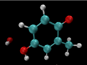
Figure 1: The hydroquionone radical (C₇H₆OOH + OH) that has been solvated in water (surrounding water is not shown).

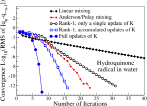
Figure 2: Convergence or the root mean square (RMS) of the difference in charge between iterations of the self-consistent-field optimization for a hydroquinone radical in water (with a total of 99 atoms and the electronic temperature $T_{e}=3,000$ K) using simple linear mixing, Anderson/Pulay mixing, rank-1 updates of the kernel $K$ or full updates of the entire $K$ in each iterations. In practice the Anderson/Pulay scheme is the fastest.

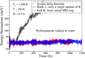
Figure 3: The fluctuations in the total free energy (potential + entropy + kinetic, corresponding to the constant of motion Eq. (41) ) of an extended Lagrangian Born-Oppenheimer molecular dynamics simulation of a hydroquinone radical in water (99 atoms, with a statistical temperature for the molecular trajectories, $T\sim 250K$, and the electronic temperature $T_{e}=3,000$ K) using three different approximations of the kernel $K$ .

The simulation of the water solvated hydroquinone radical test system in Fig. 1 is quite challenging. Even with an electronic temperature of $T_{e}=3,000$ K the initial self-consistent-field convergence can be slow. Figure 2 shows how a simple linear mixing scheme (with the fix mixing parameter optimized within a tolerance of 0.1) requires the order of 100 iterations to reach an accurate ground state solution. Anderson/Pulay mixing Banerjee et al. (2016) (without restart) accelerates convergence significantly. A rank-1 update of the kernel $K$, using the normalized perturbation vector chosen from $v_{j}=K_{j-1}(\rho[\rho_{j}]-\rho_{j})$ with the update as in Eq. (52), also offers an efficient alternative, though each iteration takes about twice as long to calculate as in the Anderson/Pulay mixing scheme. Figure 2 shows two cases of rank-1 updates, either using a single rank-1 based approximation of the kernel (each time updating a scaled delta-function estimate of $K_{0}$ in Eqs. (48) and (49) with a only single rank-1 update, Eq. (50)), or using multiple accumulated rank-1 updates, Eq. (50), one new update for each new self-consistent field iteration. The calculation with the full updates of $K$, which in each self-consistent field iteration requires as many response calculations as there are atoms in the system, converges rapidly, but is by far the slowest scheme.

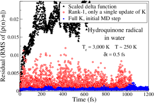
Figure 4: The the root mean square (RMS) of the residual function ($\rho[n]-n$) as a function of simulation time for the simulation of the hydroquinone radical in water in Fig. 3 .

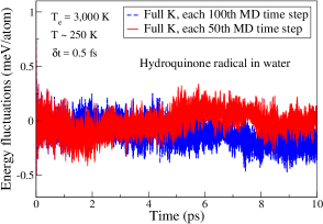
Figure 5: The fluctuations in the total free energy (potential + entropy + kinetic, corresponding to the constant of motion in Eq. (41)) of an extended Lagrangian Born-Oppenheimer molecular dynamics simulation of a hydroquinone radical in water (99 atoms).

Even if the Anderson/Pulay scheme reaches convergence in the smallest amount of wall-clock time, it seems hard to apply as approximations of the kernel $K$ in the extended Lagrangian Born-Oppenheimer molecular dynamics scheme. In this case the exact full calculation of the kernel, the rank-1 update approach (either using single rank-1 only updates of scaled delta-function approximations or accumulated rank-1 updates), or only the scaled delta-function approximation, offer better alternatives.

Figure 3 shows the fluctuations of the total free energy for an extended Lagrangian Born-Oppenheimer simulation using either a scaled delta-function approximation of the kernel, $K=cI$, the single rank-1 updated approximation of $K$, or a full calculation of the kernel in the initial time step after which $K$ is kept constant. The rank-1 and full kernel approaches have energy fluctuations that are virtually on top of each other for the first 1,000 time steps, whereas the scaled delta-function approximation shows fluctuations increasing in size, leading to a significant drift already after about 100 fs of simulation time. The behavior can be understood from the ability to keep the dynamical variable density, $n(t)$, close to the ground state, which can be estimated from the distance to $\rho[n]$, i.e. the size of the residual function $\rho[n]-n$. The root means square (RMS) of $\rho[n]-n$ is shown in Fig. 4. The simulation with the scaled delta-function approximation of $K$ shows a significant size of the residual, whereas the single rank-1 update and the full kernel approximations keep the residual function small such that $n$ remains close to the exact ground state. Using the accumulated rank-1 updated kernel (not shown) gives results similar or worse compared to the approximation using only single rank-1 updates of scaled delta-functions in each time step. The advantage with the rank-1 only (or low-rank) updated approximation of the kernel is that it can be generalized to simulations using a real-space grid, density matrices, or a plane-wave basis functions for which full kernel calculations are not practically feasible.

Figure 5 shows the total free energy of two longer molecular dynamics simulations of the hydroquinone radical in water over 10 ps of simulation time. The full kernel, updated once every 100th or 50th time step, was used as an approximation. The simulation remains stable, though it shows some long-term random-walk-like fluctuations in the total free energy due to small numerical errors in the force evaluations.

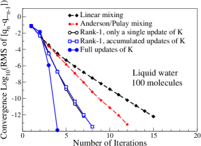
Figure 6: Convergence or the root mean square (RMS) of the difference in charge between iterations of the self-consistent-field optimization for a water system (with a total of 100 molecules at $T_{e}=3,000$ K) using simple linear mixing, Anderson/Pulay mixing, two different rank-1 updates of the kernel $K$ or full updates of the entire $K$ in each iterations. In practice the Anderson/Pulay scheme is the fastest.

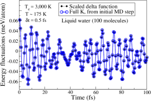
Figure 7: The fluctuations in the total free energy (potential + entropy + kinetic, corresponding to the constant of motion in Eq. (41)) of an extended Lagrangian Born-Oppenheimer molecular dynamics simulation of a water system (100 molecules) using either a scaled delta-function approximation of the kernel or the full kernel, $K$, calculated at the first time step and then kept constant. The scaled delta-function approximation and the full kernel calculation give almost identical results.

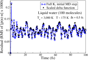
Figure 8: The root mean square (RMS) of the residual function ($\rho[n]-n$)($\times 1000$) as a function of simulation time for the water simulation in Fig. 7. The scaled delta-function approximation of the kernel $K$ and the full kernel calculation give almost identical results.

VI.2 Water

A more regular molecular dynamics simulation may be represented by liquid water. Notice, that choosing the same electronic temperature of $3,000$ K, as in the quinone system, in practice has no influence on the electronic structure of liquid water, since the gap is much larger than for the hydroquinone radical in the example above. In the liquid water simulation we find a much smaller difference between a fully optimized kernel and a scaled delta-function approximation of $K$. This is reflected in the relatively fast convergence for the simple linear mixing approach in Fig. 6. The energy fluctuation curves for the scaled delta-function kernel and the exact full kernel simulations in Fig. 7 are essentially on top of each other. The reason for this can be understood from the very small residual function, both for the scaled delta-function approximation and the exact full kernel (calculated only in the first time step and then kept fix), as shown in Fig. 8.

VI.3 Scaling analysis

By choosing an appropriate approximation of the kernel $K$, we can stabilize the dynamics of an extended Lagrangian Born-Oppenheimer molecular dynamics simulation. The kernel acts like a preconditioner in the equations of motion for the extended electronic degrees of freedom, which causes the dynamical variable density $n(t)$ to oscillate around a closer approximation of the exact Born-Oppenheimer ground state density $\rho_{\rm min}(t)$ and keeps the residual function $\rho[n]-n$ small. For many systems a simple scaled delta-function approximation of the kernel is sufficiently accurate, but for systems exhibiting slow self-consistent field convergence, the approximation based on rank-1 updates or the infrequent calculation of an exact full kernel using fractional occupation number, serve as practical alternatives, with only a modest computational overhead. A slightly more expensive alternative is to reduce the integration time step $\delta t$, which rapidly improves accuracy because of the second-order nature of extended Lagrangian Born-Oppenheimer molecular dynamics for which the residual function scales as $(\rho[n]-n)\sim\delta t^{2}$. This quadratic scaling is demonstrated in Fig. 9.

The total free energy fluctuation curves in Fig. 3 for the full kernel and the rank-1 only approximations are almost on top of each other for the first 500 fs, even if the residual functions in Fig. 4 differ in size by almost an order in magnitude. The reason for this is that the error in the free energy shadow potential compared to the fully converged regular Born-Oppenheimer free energy potential scales as $(\rho[n]-n)^{2}\sim\delta t^{4}$, whereas the amplitude of the total free energy fluctuations are dominated by the local truncation error of the Verlet scheme, which scales as $(\rho[n]-n)\sim(\rho_{\rm min}-n)\sim\delta t^{2}$. The scaling is demonstrated in Fig. 10. Any error compared to a fully converged regular Born-Oppenheimer simulation is then small compared to the error due to the finite integration time step. Figure 10, which illustrates the results from simulations of liquid nitromethane, also demonstrates the $\delta t^{2}$ scaling of the error in the forces acting on the nuclear degrees of freedom.

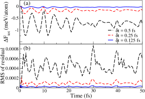
Figure 9: The upper panel (a) shows fluctuations in the total free energy (corresponding to the constant of motion in Eq. (41)) for an extended Lagrangian Born-Oppenheimer molecular dynamics simulation of the the hydroqionone radical in water for various sizes of the integration time step ($\delta t=$ 0.5 fs, 0.25 fs, and 0.125 fs). The electronic temperature was set to $T_{e}=3,000$ K and the statistical temperature of the molecular trajectories, $T\sim 250$ K. The lower panel (b) shows the corresponding fluctuations of the root mean square (RMS) of the residual function ($\rho[n]-n$). The simulations were performed with a full calculation of the kernel $K$ that was calculated for the initial configuration and then kept fix. Both the size of the fluctuations of the total free energy and the RMS of the residual function scale quadratically with the integration time step.

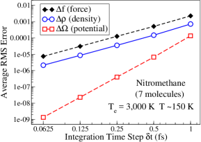
Figure 10: The scaling of the average (over $\sim 100$ fs of simulation time) of the root mean square (RMS) error, as a function of the integration time step $\delta t$, in the forces $\Delta f$, the electron density $\Delta\rho$ from ($n-\rho_{\rm min}$), and the free energy potential surface $\Delta\Omega$ from ($\Omega^{(1)}[n]({\bf R})-\Omega_{\rm BO}[\rho_{\rm min}]({\bf R})$), during an extended Lagrangian Born-Oppenheimer simulation with respect to the corresponding ”exact” fully converged Born-Oppenheimer values for each configuration, ${\bf R}(t_{0}+k\delta t)$. The deviation in the forces and the density scales as $\delta t^{2}$, whereas the error in the shadow potential scales as $\delta t^{4}$. The exact full kernel $K$ was recalculated once every 100th integration time step.

The residual function, $\rho[n]-n$, plays an important role. It provides a measure of the distance of $n(t)$ (or $\rho[n](t)$) to the exact ground state density $\rho_{\rm min}(t)$. If the residual function is too large we may expect that the validity of the linearized shadow potential energy surfaces, $U^{(1)}[n]({\bf R})$ or $\Omega^{(1)}[n]({\bf R})$, breaks down. The residual function is easy to monitor during a simulation and serves as a gauge of the accuracy in a way similar to the total free energy fluctuations. The residual function is of particular interest in simulations of canonical (NVT) ensembles that don’t necessarily have a constant of motion Martinez et al. (2015), or in simulations using linear scaling electronic structure theory for systems with fractional occupation numbers, where it might be expensive to calculate the electronic entropy.

It is not possible to demonstrate all different aspects of the kernel approximation techniques. Their relative efficiency may differ significantly depending on the test system. A wide range of tricks can also be used and combined with the kernel techniques presented here, including adaptive back tracking, variable time steps, restarts, and orthonormalized updates. The complexity, in many ways, is directly related to the challenges of the regular self-consistent field optimization for the ground state electronic structure, and we can most probably not expect a single universal black-box solver that works for all material systems in all situations.

VII What still remains

This article presents the development of extended Lagrangian Born-Oppenheimer molecular dynamics. Even if most parts of the theory seems complete several important steps are still needed, for example: 1) implementations in broadly available, state-of-the-art, first principles electronic structure codes Ahlrichs et al. (1989); Schmidt et al. (1993); Kresse and Furthmuller (1996); Hernández et al. (1996); Tsuchida and Tsukada (1998); Soler et al. (2002); Bowler et al. (2001); Ozaki and Kino (2005); VandeVondele et al. (2005); Bowler et al. (2006); Kronik et al. (2006); Bock et al. (2008); Genovese et al. (2008); Blum et al. (2009); Hine et al. (2009); Rudberg et al. (2011); VandeVondele et al. (2012); Aidas and et al. (2013); Arita et al. (2014); Osei-Kuffuor et al. (2014); Qin et al. (2015) that can take full advantage of the approximations of $K$ proposed in this paper, e.g. based on low-rank updates calculated from quantum perturbation theory; 2) convincing demonstrations of quantum-based simulations, allowing longer simulation times and/or larger system sizes than previously possible, for a broad range of problems across materials science, chemistry and biology; 3) theoretically rigorous (adaptive) integration algorithms that can be used for a variety of thermodynamic ensembles; and 4) extensions beyond regular ground state Kohn-Sham Born-Oppenheimer simulations, such as, orbital-free high-temperature methods, path-integral molecular dynamics techniques, methods for strong electron correlation, accelerated molecular dynamics, polarizable force fields and QM/MM implementations, and excited state molecular dynamics. While a few steps have been taken, a lot of work still remains.

VIII Conclusion and summary

The unified extended Lagrangian framework introduced by Car and Parrinello made first principles molecular dynamics simulations possible for a broad range of materials for the first time and set the stage for a whole generation of electronic structure modeling. In this paper I have reviewed a new approach to first principles molecular dynamics. This framework of extended Lagrangian Born-Oppenheimer molecular dynamics was presented using general Hohenberg-Kohn density functional theory and I discussed some of its similarities and differences compared to extended Lagrangian Car-Parrinello molecular dynamics. A key difference is that the accuracy of the electronic degrees of freedom in extended Lagrangian Born-Oppenheimer molecular dynamics, with respect to the exact Born-Oppenheimer solution, is of second order in the size of the integration time step and of fourth order in the potential energy surface, whereas Car-Parrinello molecular dynamics is of first order in the electronic degrees of freedom and of second order in the potential energy. This means that the underlying shadow Hamiltonian of extended Lagrangian Born-Oppenheimer molecular dynamics closely mimics the exact Born-Oppenheimer Hamiltonian. An interesting challenge is to design possibly even higher-order formulations.

Improved stability over the most recent formulation of extended Lagrangian Born-Oppenheimer molecular dynamics was achieved by generalizing the theory to finite temperature ensembles, using fractional occupation numbers in the calculation of the inner-product kernel of the harmonic oscillator extension, which appears like a preconditioner in the electronic equations of motion. I showed how this kernel can be estimated on-the-fly using rank-1 updates of approximate kernels with the updates calculated directly from quantum perturbation theory with the perturbations chosen along optimal directions, or by the exact full kernel recalculated at some low frequency. Material systems that normally exhibit slow self-consistent field convergence can be simulated using integration time steps of the same order as in direct Born-Oppenheimer molecular dynamics without the requirement of an expensive, iterative, non-linear electronic ground state optimization prior to the force evaluations and without a systematic drift in the total energy.

The formulation of extended Lagrangian Born-Oppenheimer molecular dynamics presented in this paper represents a framework for a next generation extended Lagrangian first principles molecular dynamics that overcomes shortcomings of regular, direct Born-Oppenheimer simulations, while maintaining or improving properties of Car-Parrinello molecular dynamics.

IX Acknowledgements

This work was supported by the Department of Energy Offices of Basic Energy Sciences (Grant No. LANL2014E8AN) and performed at Los Alamos National Laboratory (LANL) in New Mexico. Discussions with A. Albaugh, B. Aradi, R. Car, E. Chisolm, O. Certik, M.J. Cawkwell, Th. Frauenheim, T. Head-Gordon, S.M. Mniszewski, C.F.A. Negre, and C-K Skylaris are gratefully acknowledged as well as generous inspiration from T. Peery and the T-division international Java group. LANL, is an affirmative action/equal opportunity employer, which is operated by Los Alamos National Security, LLC, for the National Nuclear Security Administration of the U.S. DOE under Contract No. DE- AC52-06NA25396.

References

- Allen and Tildesley (1990) M. Allen and D. Tildesley, Computer Simulation of Liquids (Oxford Science, London, 1990).
- Karplus and Petsko (1990) M. Karplus and G. Petsko, Nature 347, 631 (1990).
- vanGusteren and Berendsen (1990) W. F. vanGusteren and H. J. C. Berendsen, Angewandte Chemie 29, 992 (1990).
- Tuckerman and Martyna (2000) M. E. Tuckerman and G. J. Martyna, J. Phys. Chem. B 104, 159 (2000).
- Frenkel and Smit (2002) D. Frenkel and B. Smit, “Understanding molecular simulation,” in Understanding Molecular Simulation, Second Edition (Academic Press, 2002) 2nd ed.
- Karplus and McCammon (2002) M. Karplus and J. McCammon, Nature Struc. Mol. Bio. 9, 646 (2002).
- Sanbonmatsu and Tung (2007) K. Y. Sanbonmatsu and C.-S. Tung, J. Struct. Biol. 157, 470 (2007).
- Orozco (2014) M. Orozco, Chem. Soc. Rev. 43, 5051 (2014).
- Perilla et al. (2015) J. Perilla, B. Goh, C. K. Cassidy, B. Lui, R. C. Bernardi, T. Rudack, H. Yu, Z. Wu, and K. Schulten, Curr. Opin. Struct. Biol. 31, 64 (2015).
- Marx and Hutter (2000) D. Marx and J. Hutter, “Modern methods and algorithms of quantum chemistry,” (ed. J. Grotendorst, John von Neumann Institute for Computing, Jülich, Germany, 2000) 2nd ed.
- Tuckerman (2002) M. E. Tuckerman, J. Phys.: Conden. Matter 14, 1297 (2002).
- Kirchner et al. (2012) B. Kirchner, J. di Dio Philipp, and J. Hutter, Top. Curr. Chem. 307, 109 (2012).
- Hutter (2012) J. Hutter, WIREs Comput. Mol. Sci. 2, 604 (2012).
- Wang and Karplus (1973) I. S. Y. Wang and M. Karplus, J. Am. Chem. Soc. 95, 8160 (1973).
- Leforestier (1978) C. Leforestier, J. Chem. Phys. 68, 4406 (1978).
- Warshel and Karplus (1975) A. Warshel and M. Karplus, Chem. Phys. Lett. 32, 11 (1975).
- Car and Parrinello (1985) R. Car and M. Parrinello, Phys. Rev. Lett. 55, 2471 (1985).
- Remler and Madden (1990) D. K. Remler and P. A. Madden, Mol. Phys. 70, 921 (1990).
- Pastore et al. (1991) G. Pastore, E. Smargassi, and F. Buda, Phys. Rev. A 44, 6334 (1991).
- Bornemann and Schütte (1998) F. A. Bornemann and C. Schütte, Numerische Mathematik 78, 359 (1998).
- Carloni et al. (2002) P. Carloni, U. Rothlisberger, and M. Parrinello, Acc. Chem. Res. 35, 455 (2002).
- Senn and Thiel (2009) H. M. Senn and W. Thiel, Angew. Chem. Int. Ed. Engl. 48, 1198 (2009).
- Heitler and London (1927) W. Heitler and F. London, Z. Phys. 44, 455 (1927).
- Born and Oppenheimer (1927) M. Born and R. Oppenheimer, Ann. Phys. 389, 475 (1927).
- Barnett and Landman (1993) R. N. Barnett and U. Landman, Phys. Rev. B 48, 2081 (1993).
- Kresse and Hafner (1993) G. Kresse and J. Hafner, Phys. Rev. B 47, 558 (1993).
- Pulay and Fogarasi (2004) P. Pulay and G. Fogarasi, Chem. Phys. Lett. 386, 272 (2004).
- Niklasson et al. (2006) A. M. N. Niklasson, C. J. Tymczak, and M. Challacombe, Phys. Rev. Lett. 97, 123001 (2006).
- Kühne et al. (2007) T. D. Kühne, M. Krack, F. R. Mohamed, and M. Parrinello, Phys. Rev. Lett. 98, 066401 (2007).
- Hartke and Carter (1992) B. Hartke and E. Carter, Chem. Phys. Lett. 189, 358 (1992).
- Lambert et al. (2006) F. Lambert, J. Clerouin, and S. Mazevet, Eur. Phys. Lett. 75, 681 (2006).
- Schlegel et al. (2001) H. B. Schlegel, J. M. Millam, S. S. Iyengar, G. A. Voth, A. D. Daniels, G. Scusseria, and M. J. Frisch, J. Chem. Phys. 114, 9758 (2001).
- Iyengar et al. (2001) S. S. Iyengar, H. B. Schlegel, J. M. Millam, G. A. Voth, G. Scusseria, and M. J. Frisch, J. Chem. Phys. 115, 10291 (2001).
- Herbert and Head-Gordon (2004) J. M. Herbert and M. Head-Gordon, J. Chem. Phys. 121, 11542 (2004).
- Li et al. (2016) J. Li, C. Haycraft, and S. S. Iyengar, J. Chem. Theory Comput. 12, 2493 (2016).
- Goedecker (1999) S. Goedecker, Rev. Mod. Phys. 71, 1085 (1999).
- Bowler and Miyazaki (2012) D. R. Bowler and T. Miyazaki, Rep. Prog. Phys. 75, 036503 (2012).
- Andersen (1980) H. C. Andersen, J. Chem. Phys. 72, 2384 (1980).
- Parrinello and Rahman (1980) M. Parrinello and A. Rahman, Phys. Rev. Lett. 45, 1196 (1980).
- Nose (1984) S. Nose, J. Chem. Phys. 81, 511 (1984).
- Niklasson (2008a) A. M. N. Niklasson, Phys. Rev. Lett. 100, 123004 (2008a).
- Niklasson et al. (2009) A. M. N. Niklasson, P. Steneteg, A. Odell, N. Bock, M. Challacombe, C. J. Tymczak, E. Holmstrom, G. Zheng, and V. Weber, J. Chem. Phys. 130, 214109 (2009).
- Odell et al. (2009) A. Odell, A. Delin, B. Johansson, N. Bock, M. Challacombe, and A. M. N. Niklasson, J. Chem. Phys. 131, 244106 (2009).
- Steneteg et al. (2010) P. Steneteg, I. A. Abrikosov, V. Weber, and A. M. N. Niklasson, Phys. Rev. B 82, 075110 (2010).
- Zheng et al. (2011) G. Zheng, A. M. N. Niklasson, and M. Karplus, J. Chem. Phys. 135, 044122 (2011).
- Cawkwell and Niklasson (2012) M. J. Cawkwell and A. M. N. Niklasson, J. Chem. Phys. 137, 134105 (2012).
- Souvatzis and Niklasson (2014) P. Souvatzis and A. M. N. Niklasson, J. Chem. Phys. 140, 044117 (2014).
- Niklasson and Cawkwell (2014) A. M. N. Niklasson and M. Cawkwell, J. Chem. Phys. 141, 164123 (2014).
- Aradi et al. (2015) B. Aradi, A. M. N. Niklasson, and T. Frauenheim, J. Chem. Theory Comput. 11, 3357 (2015).
- Martinez et al. (2015) E. Martinez, M. J. Cawkwell, , A. F. Voter, and A. M. N. Niklasson, J. Chem. Phys. 142, 1770 (2015).
- Vitale et al. (2017) V. Vitale, J. Dziezic, A. Albaugh, A. Niklasson, T. J. Head-Gordon, and C.-K. Skylaris, J. Chem. Phys. 12, 124115 (2017).
- Albaugh et al. (2017) A. Albaugh, A. Niklasson, and T. J. Head-Gordon, J. Phys. Chem. Lett. 8, 1714 (2017).
- Lin et al. (2014) L. Lin, J. Lu, and S. Shao, Entropy 16, 110 (2014).
- Herbert and Head-Gordon (2005) J. Herbert and M. Head-Gordon, Phys. Chem. Chem. Phys. 7, 3269 (2005).
- Kolafa (2003) J. Kolafa, J. Comput. Chem. 25, 335 (2003).
- Niklasson et al. (2011) A. M. N. Niklasson, P. Steneteg, and N. Bock, J. Chem. Phys. 135, 164111 (2011).
- Arita et al. (2014) M. Arita, D. R. Bowler, and T. Miyazaki, J. Chem. Theory Comput. 10, 5419 (2014).
- Nomura et al. (2015) K. Nomura, P. E. Small, R. K. Kalia, A. Nakano, and P. Vashista, Comput. Phys. Comm. 192, 91 (2015).
- Albaugh et al. (2015) A. Albaugh, O. Demardash, and T. J. Head-Gordon, J. Chem. Phys. 143, 174104 (2015).
- Niklasson et al. (2016) A. M. N. Niklasson, S. M. Mnizsewski, C. F. A. Negre, M. J. Cawkwell, P. J. Swart, J. Mohd-Yusof, T. C. Germann, M. E. Wall, N. Bock, E. H. Rubensson, and H. Djidjev, J. Chem. Phys. 144, 234101 (2016).
- Levy (1979) M. Levy, Proc. Nat. Acad. Sci. 76, 6062 (1979).
- Lieb (1983) E. H. Lieb, Int. J. Quant. Chem. 24, 243 (1983).
- Hohenberg and Kohn (1964) P. Hohenberg and W. Kohn, Phys. Rev. 136, B:864 (1964).
- Parr and Yang (1989) R. G. Parr and W. Yang, Density-functional theory of atoms and molecules (Oxford University Press, Oxford, 1989).
- Dreizler and Gross (1990) R. Dreizler and K. Gross, Density-functional theory (Springer Verlag, Berlin Heidelberg, 1990).
- Broyden (1965) C. G. Broyden, Math. Comput. 19, 577 (1965).
- Anderson (1965) D. G. Anderson, J. Assoc. Comput. Mach. 12, 547 (1965).
- Pulay (1980) P. Pulay, Chem. Phys. Let. 73, 393 (1980).
- Srivastava (1984) G. P. Srivastava, J. Phys. A: Math. Gen. 17, L317 (1984).
- Kerker (1981) G. P. Kerker, Phys. Rev. B 23, 3082 (1981).
- Johnson (1988) D. D. Johnson, Phys. Rev. B 38, 12807 (1988).
- Fletcher (1970) R. Fletcher, Mol. Phys. 19, 55 (1970).
- Stich et al. (1989) I. Stich, R. Car, M. Parrinello, and S. Baroni, Phys. Rev. B 39, 4997 (1989).
- Hutter et al. (1994) J. Hutter, H. P. Luthi, and M. Parrinello, Comput. Mater. Sci 2, 244 (1994).
- Weber et al. (2008) V. Weber, J. VandeVondele, J. Hutter, and A. M. N. Niklasson, J. Chem. Phys. 128, 084113 (2008).
- Channel and Scovel (1990) J. P. Channel and C. Scovel, Nonlinearity 3, 231 (1990).
- McLachlan and Atela (1992) R. McLachlan and P. Atela, Nonlinearity 5, 541 (1992).
- Leimkuhler and Reich (2004) B. Leimkuhler and S. Reich, Simulating Hamiltonian Dynamics (Cambridge University Press, Cambridge, 2004).
- Engel et al. (2005) R. D. Engel, R. D. Skeel, and M. Drees, J. Comput. Phys. 206, 432 (2005).
- Harris (1985) J. Harris, Phys. Rev. B 31, 1770 (1985).
- Foulkes and Haydock (1989) W. M. C. Foulkes and R. Haydock, Phys. Rev. B 39, 12520 (1989).
- Negre et al. (2016) C. F. A. Negre, S. M. Mnizsewski, A. M. N. Niklasson, S. M. Mnizsewski, M. J. Cawkwell, N. Bock, M. E. Wall, and A. M. N. Niklasson, J. Chem. Theory Comput. 12, 3063 (2016).
- Hirakawa et al. (2017) T. Hirakawa, T. suzuki, D. R. Bowler, and T. Myazaki, arXiv http://arxiv.org/abs/1705.01448 (2017).
- Pecora and Carrol (1990) L. M. Pecora and T. L. Carrol, Phys. Rev. Lett. 64, 821 (1990).
- Pecora and Carrol (2015) L. M. Pecora and T. L. Carrol, Chaos 25, 097611 (2015).
- Odell et al. (2011) A. Odell, A. Delin, B. Johansson, M. J. Cawkwell, and A. M. N. Niklasson, J. Chem. Phys. 135, 224105 (2011).
- Tangney and Scandolo (2002) P. Tangney and S. Scandolo, J. Chem. Phys. 116, 14 (2002).
- Tangney (2006) P. Tangney, J. Chem. Phys. 124, 44111 (2006).
- Souvatzis and Niklasson (2013) P. Souvatzis and A. M. N. Niklasson, J. Chem. Phys. 139, 214102 (2013).
- Mermin (1965) N. D. Mermin, Phys. Rev. B 137, A1441 (1965).
- Weinert and Davenport (1992) M. Weinert and J. W. Davenport, Phys. Rev. B 45, R13709 (1992).
- Wentzcovitch et al. (1992) R. M. Wentzcovitch, J. L. Martins, and P. B. Allen, Phys. Rev. B 45, R11372 (1992).
- Niklasson (2008b) A. M. N. Niklasson, J. Chem. Phys. 129, 244107 (2008b).
- Nishimoto (2017) Y. Nishimoto, J. Chem. Phys. 146, 084101 (2017).
- Niklasson and Challacombe (2004) A. M. N. Niklasson and M. Challacombe, Phys. Rev. Lett. 92, 193001 (2004).
- Weber et al. (2004) V. Weber, A. M. N. Niklasson, and M. Challacombe, Phys. Rev. Lett. 92, 193002 (2004).
- Weber et al. (2005) V. Weber, A. M. N. Niklasson, and M. Challacombe, J. Chem. Phys. 123, 44106 (2005).
- Niklasson et al. (2015) A. M. N. Niklasson, M. J. Cawkwell, E. H. Rubensson, and E. Rudberg, Phys. Rev. E 92, 063301 (2015).
- Sherman and Morrison (1950) J. Sherman and W. J. Morrison, Ann. Math. Statist. 21, 124 (1950).
- Elstner et al. (1998) M. Elstner, D. Poresag, G. Jungnickel, J. Elsner, M. Haugk, T. Frauenheim, S. Suhai, and G. Seifert, Phys. Rev. B 58, 7260 (1998).
- Finnis et al. (1998) M. W. Finnis, A. T. Paxton, M. Methfessel, and M. van Schilfgarde, Phys. Rev. Lett. 81, 5149 (1998).
- Frauenheim et al. (2000) T. Frauenheim, G. Seifert, M. E. aand Z. Hajnal, G. Jungnickel, D. Poresag, S. Suhai, and R. Scholz, Phys. Stat. sol. 217, 41 (2000).
- Cawkwell and et al. (2010) M. J. Cawkwell and et al., “LATTE,” (2010), Los Alamos National Laboratory (LA- CC-10004), http://www.github.com/lanl/latte.
- Sanville et al. (2010) E. Sanville, N. Bock, W. M. Challacombe, A. M. N. Niklasson, M. J. Cawkwell, D. M. Dattelbaum, and S. Sheffield, “Proceedings of the fourteenth international detonation symposium,” (Office of Naval Research, Arlington VA, ONR-351-10-185, 2010) pp. 91–101.
- Pulay (1982) P. Pulay, J. Comput. Chem. 3, 556 (1982).
- Banerjee et al. (2016) A. S. Banerjee, P. Suryanaryana, and J. E. Pask, Chem. Phys. Lett. 647, 31 (2016).
- Ahlrichs et al. (1989) R. Ahlrichs, M. Bär, M. Häser, H. Hom, and C. Kölmel, Chem. Phys. Lett. 162, 165 (1989).
- Schmidt et al. (1993) M. W. Schmidt, K. K. Baldridge, J. A. Boatz, S. T. Elbert, M. S. Gordon, J. H. Jensen, S. Koseki, N. Matsunaga, K. A. Nguyen, S. J. Su, T. L. Windus, M. Dupuis, and J. A. Montgomery, J. Comput. Chem. 14, 1347 (1993).
- Kresse and Furthmuller (1996) G. Kresse and J. Furthmuller, Phys. Rev. B 54, 11169 (1996).
- Hernández et al. (1996) E. Hernández, M. J. Gillan, and C. Goringe, Phys. Rev. B 53, 7147 (1996).
- Tsuchida and Tsukada (1998) E. Tsuchida and M. Tsukada, J. Phys. Soc. Jpn. 67, 340 (1998).
- Soler et al. (2002) J. M. Soler, E. Artacho, J. D. Gale, A. Garcia, J. Junquera, P. Ordejon, and D. Sanchez-Portal, J. Phys.: Condens. Matter 14, 2745 (2002).
- Bowler et al. (2001) D. R. Bowler, T. Miyazaki, and M. Gillan, Comput. Phys. Comm. 137, 255 (2001).
- Ozaki and Kino (2005) T. Ozaki and H. Kino, Phys. Rev. B 72, 045121 (2005).
- VandeVondele et al. (2005) J. VandeVondele, M. Krack, F. Mohammed, M. Parrinello, T. Chassing, and J. Hutter, Comput. Phys. Commun. 167, 103 (2005).
- Bowler et al. (2006) D. R. Bowler, R. Choudhury, M. J. Gillan, and T. Miyazaki, Phys. Stat. Sol. B 243, 898 (2006).
- Kronik et al. (2006) L. Kronik, A. Makmal, M. Tiago, M. M. Alemany, X. Huang, and Y. Saad, Phys. Stat. Solidi. 243, 1063 (2006).
- Bock et al. (2008) N. Bock, M. Challacombe, C. K. Gan, G. Henkelman, K. Nemeth, A. M. N. Niklasson, A. Odell, E. Schwegler, C. J. Tymczak, and V. Weber, “FreeON,” (2008), Los Alamos National Laboratory (LA-CC 01-2; LA- CC-04-086), Copyright University of California.
- Genovese et al. (2008) L. Genovese, A. Neelov, S. Goedecker, T. Deutsch, S. A. Ghasemi, A. Willand, D. Caliste, O. Zilerberg, M. Rayson, A. Bergman, and R. Schneider, J. Chem. Phys. 129, 014109 (2008).
- Blum et al. (2009) V. Blum, R. Gehrke, F. Hanke, P. Havu, V. Havu, X. Ren, K. Reuter, and M. Sheffler, Comput. Phys. Commun. 180, 2175 (2009).
- Hine et al. (2009) N. D. Hine, P. D. Haynes, A. A. Mostofi, C.-K. Skylaris, and M. C. Payne, Comput. Phys. Comm. 180, 1041 (2009).
- Rudberg et al. (2011) E. Rudberg, E. H. Rubensson, and P. Salek, J. Chem. Theory Comput. 7, 340 (2011).
- VandeVondele et al. (2012) J. VandeVondele, U. Borstnik, and J. Hutter, J. Chem. Theory Comput. 8, 3565 (2012).
- Aidas and et al. (2013) K. Aidas and et al., WIREs Comput. Mol. Sci. 4, 269 (2013).
- Osei-Kuffuor et al. (2014) D. Osei-Kuffuor, J. L. Fattebert, and F. Gygi, Phys. Rev. Lett. 112, 046401 (2014).
- Qin et al. (2015) X. M. Qin, H. H. Shang, H. J. Xiang, Z. Y. Li, and J. L. Yang, Int. J. Quantum Chem. 115, 647 (2015).