Detecting topology change via correlations and entanglement

from gauge/gravity correspondence

Hai Lin¹, Keyou Zeng²

¹Yau Mathematical Sciences Center, Tsinghua University, Beijing 100084, P. R. China

²Department of Physics, Tsinghua University, Beijing 100084, P. R. China

We compute a momentum space version of the entanglement spectrum and entanglement entropy of general Young tableau states, and one-point functions on Young tableau states. These physical quantities are used to measure the topology of the dual spacetime geometries in the context of gauge/gravity correspondence. The idea that Young tableau states can be obtained by superposing coherent states is explicitly verified. In this quantum superposition, a topologically distinct geometry is produced by superposing states dual to geometries with a trivial topology. Furthermore we have a refined bound for the overlap between coherent states and the rectangular Young tableau state, by using the techniques of symmetric groups and representations. This bound is exponentially suppressed by the total edge length of the Young tableau. It is also found that the norm squared of the overlaps is bounded above by inverse powers of the exponential of the entanglement entropies. We also compute the overlaps between Young tableau states and other states including squeezed states and multi-mode entangled states which have similarities with those appeared in quantum information theory.

1 Introduction

The gauge/gravity correspondence [1, 2, 3] is a nontrivial duality between a quantum system without gravity and a quantum theory incorporating gravity in the bulk. It provides a model for studying quantum gravity by quantum field theory on the boundary of the spacetime. The duality reveals the emergence of spacetime geometry from the degrees of freedom on the asymptotic boundary, and the bulk spacetime emerges dynamically from the quantum mechanical description that lives in fewer dimensions [4, 5, 6, 7]. The most studied example of gauge/gravity correspondence is an exact equivalence between Type-IIB String Theory on $AdS_{5}\times S^{5}$ and $\mathcal{N}=4$ Supersymmetric Yang-Mills Theory (SYM) on $4$-$d$ Minkowski spacetime. This correspondence allows us to perform calculations relevant to the string theory while working in the quantum field theory side. It further provides us a way to investigate new quantitative features of non-perturbative effect in quantum gravity, and it greatly enriches our knowledge about non-perturbative aspects of string theory.

In the context of gauge/gravity correspondence, there are backreacted geometries that correspond to highly excited states in the field theory side, such as the bubbling geometries [8, 9, 10]. On the gravity side, they have complicated topologies and geometries, and have interesting features including backreaction and topology changes [8, 6]. On the field theory side, states in the Hilbert space of the quantum field theory are explicitly mapped to the gravity side by associating the corresponding droplet configuration to the boundary value at the interior of the spacetimes [9, 10, 8].

Study in the field theory side shows that these different configurations [8, 9, 10] live in the same Hilbert space. Different geometries correspond to excited states which are treated on equal footing. Since they live in the same Hilbert space, one can perform operations that are allowed by quantum mechanics, and can superpose states and compute transition probabilities between different states, for example [11, 12, 13]. Different microstates can be distinguished from each other, by looking carefully at correlation functions [14, 15, 16].

In this paper we focus on states which possess interesting geometric properties in the gravity side. One class of known examples are composite states labeled by Young tableaux, also called Young tableau states. Their geometric properties in the gravity side are known to us [8, 9, 10]. Another interesting type of states are coherent states [11]. The coherent states are interesting, since the gravity dual of these states have descriptions in terms of semiclassical geometries [8, 9, 10]. There are some interesting phenomena related to these two kind of states. As pointed out in [11] and further verified in our paper that while the coherent states around vacuum have trivial topology, after superposing them, one can produce Young tableau states dual to geometries with a distinct topology. Besides, the number of annuli of the geometries can be independently predicted from the field theory side [11]. In this paper we analyze measuring topology and detecting topology change, via correlations and entanglement in the context of gauge/gravity correspondence. Topology change is important and should be taken into account in a quantum theory of gravity for consistency reasons [17, 18, 19]. In order to understand the transition probabilities from the coherent states to Young tableau states, we need to compute the overlaps between them, and this is what we have done in this paper. The probabilities calculated from these overlaps describe the probabilities of topology-changing transition from the geometry with a trivial topology to the geometry with a distinct non-trivial topology. For instance, during this transition, the number of the black annuli in the geometries has changed. These configurations also have similarities with the fuzzballs [20], which have provided important insights into the information loss problem.

Quantum entanglement is a generic feature of a many-body quantum system. Quantum correlations are also an important resource for information processing, and are important in quantum information theory [21]. In our study of the gauge/gravity correspondence, the quantum field theory side of the duality is an example of a many-body quantum system. This also indicates that many-body states are very important in the field theory side. Indeed, there are states that are of interest both in our setup and in quantum information theory, which will be discussed in our paper. Among other things, we compute a momentum space version of the entanglement spectrum and entanglement entropy of Young tableau states.

The theory of the symmetric group naturally arises in the study of many-body quantum mechanics since the permutation of particles naturally defines an action of symmetric group on the Hilbert space. Also, there is a useful way to label many-body identical particles by using symmetric groups. We will study heavy states labeled by Young tableaux corresponding to the representations of symmetric groups. Mathematically speaking, the approach and derivation here use the techniques of symmetric groups and the theories of representations and characters [22, 23, 24, 25, 26, 10]. From a mathematical point of view, the study of the symmetric group is intimately related to the theory of symmetric functions. Therefore, we see that the symmetric function theory is a powerful tool in our study of quantum many-body physics. On the other hand, physical intuition may also lead to new insights into mathematics. And we will present such an example that relates the characters of the symmetric group to the topological properties of the bubbling geometry.

The organization of this paper is as follows. In Section 2, we describe general Young tableau states and their entanglement spectrum and entanglement entropy. In Section 3, we compute the inner product between coherent states and Young tableau states. Afterwards in Section 4, we analyze the bound of the overlap between coherent states and Young tableau states. And then in Section 5, we construct a generalized expansion formula for general Young tableau states in integral representation. In Section 6, we discuss squeezed states and multi-mode entangled states and their overlaps with Young tableau states. Finally, we discuss our results and draw some conclusions in Section 7.

2 Young tableau states and entanglement

Quantum entanglement is a common feature of a many-body quantum system. Many-body states are important in the study of the gauge/gravity duality. In our setup, composite many-body states can be labeled by Young tableaux, in which the tableaux [25] keep track of appropriate symmetrization of various indices of many identical particles. Here we consider the composite states, which are labeled by Young tableaux and sometimes called Young tableau states. They are not direct product states and we consider their entanglement entropy.

Let us begin by describing the Hilbert space in our discussion. The Hilbert space of states have a nature tensor product structure given by the momentum number $k,$

$$\mathcal{H}=\bigotimes_{k}\mathcal{H}_{k}=\mathcal{H}_{1}\otimes\mathcal{H}_{2}\otimes\dots,$$ (2.1)

where $\mathcal{H}_{k}$ is the Hilbert space for mode $k$. The creation and annihilation operators for mode $k$ are $a_{k}^{\dagger}$ and $a_{k}$. Their commutation relations are

$$[a_{k},~{}a_{k^{\prime}}^{\dagger}]=k\delta_{kk^{\prime}},$$ (2.2)

with appropriate normalization convention. The states in mode $k$, with occupation number $l$, is $t_{k}^{l}=(a_{k}^{\dagger})^{l}\left|0\right\rangle_{k},$where $\left|0\right\rangle_{k}~{}$is the vacuum of $\mathcal{H}_{k}$. Constructions in this section work generally for systems having a similar Hilbert space, but we mention that in the context of half BPS sector of the SYM in which gauge invariant observables can be constructed from a single complex matrix $X$, the $t_{k}$ corresponds to $\text{Tr}(X^{k})$.

We can also understand this Hilbert space in terms of the conjugacy classes [23, 24] of the symmetric group. Here $t_{k}$ represents a conjugacy class of cycle of length $k$. The $\mathcal{H}_{k}$ is spanned by $t_{k}^{w_{k}},\;w_{k}=0,1,2\dots$, where $w_{k}$ is the occupation number for mode $k$. The states $t_{k}^{w_{k}}$ have also been studied in [11, 10, 9, 8, 22, 27, 28, 29, 30]. A general conjugacy class can be written as $\prod_{k}t_{k}^{w_{k}}$. In other words, a conjugacy class is uniquely determined and labeled by a sequence $\vec{w}=(w_{1},w_{2},\dots)$. States in the Hilbert space $\mathcal{H}$ can be spanned by the basis

$$\prod_{k}(t_{k})^{w_{k}}:=\prod_{k}\left(a_{k}^{\dagger}\right)^{w_{k}}\left|0\right\rangle,$$ (2.3)

where $\left|0\right\rangle=\otimes_{k}\left|0\right\rangle_{k}$ is the vacuum of $\mathcal{H}$. Hence the states $\prod_{k}t_{k}^{w_{k}}$ live in $\mathcal{H}$, with each factor $t_{k}^{w_{k}}$ lives in the subspace$~{}\mathcal{H}_{k}$. The norm is

$$\parallel\prod_{k}t_{k}^{w_{k}}\parallel^{2}=\prod_{k}k^{w_{k}}w_{k}!,$$ (2.4)

and the inner product $\langle\prod_{k}t_{k}^{w_{k}}\lvert\prod_{k}t_{k}^{u_{k}}\rangle=0$ if $\vec{w}\neq\vec{u}$. The factor $k^{w_{k}}$ is due to the $k$ in the convention of the commutation relation (2.2). In this paper, we sometimes use the symbol $\left|{t_{k}^{l}}\right\rangle$ to denote the same state ${t_{k}^{l}}$, and we also denote $\prod_{k}{t_{k}^{w_{k}}}$ to mean $\otimes_{k}{t_{k}^{w_{k}}}$, where the products of states are understood as tensor products.

For a Young tableau $\lambda$, we write $\lambda\vdash n$ to mean that $\lambda$ corresponds to a partition of $n$. From the representation theory of symmetric group, we know that each Young tableau $\lambda$ is associated with an irreducible representation of the symmetric group $S_{n}$. We define a Young tableau state that is associated with the Young tableau $\lambda$ by

$$\left|\lambda\right\rangle=\sum_{\vec{w}\in p(n)}\chi_{\lambda}(\vec{w})\prod_{k}\frac{1}{k^{w_{k}}w_{k}!}(t_{k})^{w_{k}},$$ (2.5)

where $p(n)$ is the set of all partitions of $n$, which is all such $\vec{w}$ that $\sum kw_{k}=w_{1}+2w_{2}+3w_{3}+\dots=n$. Here $\vec{w}$ denotes a partition and also a conjugacy class. Here $\chi_{\lambda}$ is the character [24] of the irreducible representation associated with $\lambda$, and $\chi_{\lambda}(\vec{w})$ means the value of the character on the conjugacy class $\vec{w}$, or $\chi_{\lambda}(\prod_{k}t_{k}^{w_{k}})$. We can view a general Young tableau as a multipartite system, as it can be expanded by different conjugacy classes of cycles with various lengths.

These states are dual to bubbling geometries with various droplet configurations [8$-$12, 14, 31$-$34]. See Figure 1 (a). The LLM bubbling geometries contain a black and white plane. There is a time direction and a radial direction perpendicular to this plane. And there is $S^{3}\times S^{3}$ fibered over the black and white plane. One $S^{3}$ shrinks smoothly on the black domains and the other $S^{3}$ shrinks smoothly on the white domains.

(a) State dual to the rectangular Young tableau

(b) State with more symmetry

(c) State with less symmetry

Figure 1: This is the black and white plane inside the ten-dimensional LLM bubbling geometries in string theory. The droplet picture of the geometry dual to the operator labeled by a Young tableau on the field theory side is shown in (a). The droplet picture of the geometries dual to the operators corresponding to the coherent states on the field theory side are shown in (b, c). The geometries corresponding to states (b) and (c) have the same topology as the ground state geometry. While, the geometry corresponding to (a) has a different topology. On the other hand, the states represented by (b) and (c) participate in the superposition to obtain state (a).

Given a Young tableau state $\rvert\lambda\rangle$, it can be mapped to a droplet configuration, where horizontal edges correspond to white annuli and vertical edges correspond to black annuli. And the area of the annulus is determined by the length of the corresponding edge. The operator $\frac{1}{\sqrt{j^{l}l!}}(a_{j}^{\dagger})^{l}$ creates excitations whose gravity dual interpretations are $l$ Kaluza-Klein (KK) gravitons each with momentum $j$, moving along the circular direction on the black and white plane in the bubbling geometries [8]. We denote the length of each horizontal edge to be $L_{i}$, and the length of each vertical edge to be $M_{i}$. Then the corresponding white and black annuli have areas $L_{i}$ and $M_{i}$. The corresponding droplets are shown in Figure 2.

Figure 2: More general Young tableau and the corresponding droplets.

There is another type of states, the coherent states [11]. A general coherent state can be written as

$$\left|Coh\right\rangle =\prod_{k}\exp(\Lambda_{k}\frac{t_{k}}{k})=\prod_{k}(\sum_{l_{k}=0}^{\infty}\frac{1}{l_{k}!}(\Lambda_{k}\frac{t_{k}}{k})^{l_{k}})$$

$$=\sum_{\vec{l}}\prod_{k}\frac{1}{l_{k}!}(\Lambda_{k}\frac{t_{k}}{k})^{l_{k}}$$ (2.6)

where $\Lambda_{k}$ are parameters of the coherent states, and the last sum is over all $\vec{l}=(l_{1},l_{2},\dots)$. Coherent states can also be mapped to the droplet configuration. They can describe ripples or deformations with various sizes around vacuum configuration. See Figure 1 (b, c) for example.

The Young tableau state $\left|\lambda\right\rangle$ is not a direct product state, and hence it has nonzero entanglement between modes. Their entanglement entropy can be calculated by explicit partial tracing in the Hilbert space. Consider the subsystem whose Hilbert space is $\mathcal{H}_{j}$, here $j$ parametrizes different modes in the momentum space. The entanglement entropy for a composite Young tableau state $\left|\lambda\right\rangle$ (where $\lambda\vdash n$) is

$$s_{j}(\lambda)=-\ \mathrm{Tr}\ _{\mathcal{H}_{j}}(\hat{\rho_{j}}\log(\hat{\rho_{j}})),$$ (2.7)

where

$$\hat{\rho_{j}}=\hat{\rho_{j}}(\lambda)=\ \mathrm{Tr}_{j}(\left|\lambda\right\rangle\left\langle\lambda\right|).$$ (2.8)

Here $\hat{\rho_{j}}=\hat{\rho_{j}}(\lambda)$ is the density matrix operator for the subsystem whose Hilbert space is $\mathcal{H}_{j}$. And Eq. (2.7) is the entanglement entropy in momentum space of the subsystem whose Hilbert space is $\mathcal{H}_{j}$, and is obtained by tracing out other subsystems that are complement to it, whose Hilbert space is $\bigotimes_{k\neq j}\mathcal{H}_{k}$. This is the momentum space version of the entanglement entropy. It is useful for studying UV/IR entanglement, where UV and IR modes are entangled. The subsystem in this case, is a region in the momentum space. The individual Young tableau state is a pure state. The entanglement entropy $s_{j}$ arises after partial tracing out other momentum modes living in the momentum space version of the Hilbert space decomposition. In the calculation of the entropy, we will calculate partial trace, and we write $\mathrm{Tr}_{k}$ to mean tracing over $\bigotimes_{j\neq k}\mathcal{H}_{j}$, or in other words $\mathrm{Tr}_{k}=\mathrm{Tr}\ _{\otimes_{j\neq k}\mathcal{H}_{j}}$. This has to be distinguished from $\mathrm{Tr}\ _{\mathcal{H}_{k}}$ in our notation. These density matrices and their associated entanglement entropies can be calculated by using correlation functions or inner products $\langle\lambda\lvert\prod_{k}{t_{k}^{w_{k}}}\rangle$.

Let us compute

$$\hat{\rho_{j}}(\lambda) =\ \mathrm{Tr}_{j}(\left|\lambda\right\rangle\left\langle\lambda\right|)$$

$$=\ \mathrm{Tr}_{j}(\sum_{\vec{w}\in p(n)}\chi_{\lambda}(\vec{w})\sum_{\vec{u}\in p(n)}\chi_{\lambda}(\vec{u})\prod_{k}\frac{1}{k^{w_{k}}w_{k}!}\frac{1}{k^{u_{k}}u_{k}!}\left|{t_{k}^{w_{k}}}\right\rangle\left\langle{t_{k}^{u_{k}}}\right|).$$ (2.9)

While tracing over $\bigotimes_{k\neq j}\mathcal{H}_{k}$, since $\mathrm{Tr}\ _{\mathcal{H}_{k}}(\left|{t_{k}^{w_{k}}}\right\rangle\left\langle{t_{k}^{u_{k}}}\right|)=\langle t_{k}^{u_{k}}\lvert t_{k}^{w_{k}}\rangle$, so we have

$$\mathrm{Tr}\ _{j}(\prod_{k}\left|{t_{k}^{w_{k}}}\right\rangle\left\langle{t_{k}^{u_{k}}}\right|)=\left|{t_{j}^{w_{j}}}\right\rangle\left\langle{t_{j}^{u_{j}}}\right|\prod_{k\neq j}k^{w_{k}}w_{k}!\delta_{w_{k},u_{k}}~{}.$$ (2.10)

The vector $\left|{t_{j}^{w_{j}}}\right\rangle~{}$has to be normalized in order to calculate the entropy. Define $\left|w{{}_{j}}\right\rangle_{j}=\frac{1}{\sqrt{j^{w_{j}}w_{j}!}}\left|{t_{j}^{w_{j}}}\right\rangle$, this normalized state has norm 1. Then the density matrix can be written as

$$\hat{\rho_{j}}(\lambda)=\sum_{\vec{w}\in p(n)}(\chi_{\lambda}(\vec{w}))^{2}(\prod_{k\neq j}(\frac{1}{k^{w_{k}}w_{k}!}))\frac{1}{j^{w_{j}}w_{j}!}\left|w{{}_{j}}\right\rangle_{j}\left\langle w{{}_{j}}\right|_{j},$$ (2.11)

where $p(n)~{}$is the set of all partitions of $n$.

We can read out the probability distribution from this expression

$$p_{l}^{(j)}(\lambda)=\sum_{\vec{w}\in p(n),w_{j}=l}(\chi_{\lambda}(\vec{w}))^{2}(\prod_{k\neq j}(\frac{1}{k^{w_{k}}w_{k}!}))\frac{1}{j^{l}l!}~{}.$$ (2.12)

The $p_{l}^{(j)}(\lambda)$ are the non-zero eigenvalues of the density matrix $\hat{\rho}_{j}(\lambda)$. The $p_{l}^{(j)}(\lambda)$ is also the probability for mode $j$ to have occupation number $l$, for a given Young tableau $\lambda$. The number of none-zero eigenvalues of $\hat{\rho_{j}}$ is bounded from above by $n$, which is the total number of boxes of the Young tableau $\lambda$. The Eq. (2.12) is the entanglement spectrum of a general Young tableau $\lambda$. The $p_{l}^{(j)}$ are the corresponding probability distributions, and they depend on the representation $\lambda$, that is $p_{l}^{(j)}=p_{l}^{(j)}(\lambda)$. The density matrices $\hat{\rho}_{i}(\lambda)$ are density matrices living in the space of Young tableaux.

The characters have the orthogonality relation

$$\sum_{\vec{w}\in p(n)}\frac{\chi_{\lambda}(\vec{w})\chi_{\mu}(\vec{w})}{\prod_{k}k^{w_{k}}w_{k}!}=\delta_{\lambda,\mu},$$ (2.13)

or specifically

$$\sum_{\vec{w}\in p(n)}\frac{\chi_{\lambda}(\vec{w})^{2}}{\prod_{k}k^{w_{k}}w_{k}!}=1.$$ (2.14)

We have hence shown that $\sum_{l}p_{l}^{(j)}=1.$

Hence the entropy is

$$s_{i}(\lambda)=-\sum_{l}p_{l}^{(i)}(\lambda)\log(p_{l}^{(i)}(\lambda))$$ (2.15)

and this is for a general Young tableau state labeled by $\lambda$.

Theorem 2.1.

For any Young tableau $\lambda$, define the transpose of $\lambda$, $\lambda^{T}$ to be the Young tableau whose shape is given by reflecting the original diagram $\lambda$ along its main diagonal. Then the states defined by $\lambda$ and $\lambda^{T}$ have the same entanglement spectrum, and hence the same entanglement entropy.

Proof.

The Specht modules $V^{\lambda}$ of symmetric group have the following property

$$V^{\lambda}\cong V^{(1^{n})}\otimes V^{\lambda^{T}},$$ (2.16)

where $V^{(1^{n})}$ corresponds to the sign representation. This gives us a formula for the character

$$\chi_{\lambda}(\vec{w})=sgn(\vec{w})\chi_{\lambda^{T}}(\vec{w}).$$ (2.17)

Since $sgn(\vec{w})=\pm 1$, this means that the square of the characters for two tableaux conjugate to each other is the same,

$$(\chi_{\lambda}(\vec{w}))^{2}=(\chi_{\lambda^{T}}(\vec{w}))^{2}.$$ (2.18)

Using the expression for probability distribution

$$p^{(j)}_{l}(\lambda)=\sum_{\begin{subarray}{c}w_{1},\dots,w_{j-1},w_{j+1},\dots,w_{n};\\ w_{1}+\dots+lj+\dots+nw_{n}=n\end{subarray}}(\chi_{\lambda}(\vec{w}))^{2}(\prod_{k\neq j}\frac{1}{k^{w_{k}}w_{k}!})(\frac{1}{j^{l}l!}),$$ (2.19)

it follows straightforwardly that

$$p^{(j)}_{l}(\lambda)=p^{(j)}_{l}(\lambda^{T}).$$ (2.20)

This also proves that they have the same entanglement entropy $s_{j}(\lambda)=s_{j}(\lambda^{T})$. ∎

In passing, we mention that the coherent state (2.6) can be written as

$$\rvert Coh\rangle=\bigotimes_{s=1}^{\infty}\exp(\Lambda_{s}\frac{a_{s}^{\dagger}}{s})\rvert 0\rangle_{s}.$$ (2.21)

It’s a general fact that a tensor product state has no entanglement between modes. Therefore the coherent state here, which can be viewed as a momentum space version of the coherent state, is a special case of this general result and has zero entropy for each mode. Note that there are also other types of coherent states [32] in real space, which are different from the ones we consider here.

2.1 Single row and single column states

Let us now look at simplest Young tableaux, those with a single row or a single column. Then we will move on to discuss Young tableaux with more complicated shapes. The state $\left|\lambda\right\rangle$ whose Young tableau is a single row with length $n$, is called a single row state, denoted as $\left|\Delta\right\rangle_{n}$. This correspond to the totally symmetric representation with $\chi_{\lambda}(\vec{w})=1$. From the expression (2.12) above, and using some combinatoric techniques, the probability for occupation number $l$ in mode $j$ is

$$p_{l}^{(j)}(n)=\frac{1}{l!j^{l}}\sum_{k=0}^{\lfloor\frac{n-jl}{j}\rfloor}\frac{(-1)^{k}}{k!j^{k}}.$$ (2.22)

The entanglement entropy is

$$s_{j}(n)=\sum_{l=0}^{n}-p_{l}^{(j)}(n)\log p_{l}^{(j)}(n).$$ (2.23)

Using Incomplete Gamma function $\Gamma(s,x):=\int_{x}^{\infty}t^{s-1}e^{-t}\mathrm{d}t$, the probability can be written as

$$p_{l}^{(j)}(n)=\frac{\Gamma(1+\lfloor\frac{n-jl}{j}\rfloor,\frac{-1}{j})}{e^{1/j}j^{l}\Gamma(1+l)\Gamma(1+\lfloor\frac{n-jl}{j}\rfloor)}.$$ (2.24)

The expression can be simplified in large $n$ limit, and we always assume a large $n$ limit in the rest of this section. For large $n$, the expression for the probability distribution can be simplified as

$$p_{l}^{(j)}=\frac{1}{l!j^{l}}e^{-\frac{1}{j}},$$ (2.25)

where we used $p_{l}^{(j)}$ to represent the probability for large $n$. This is a Poisson distribution with Fisher information being $j$. Consider $\lim_{n\rightarrow\infty}s_{j}(n)=s_{j}$,

$$s_{j}=\frac{1}{j}+\sum_{l=0}^{\infty}e^{-1/j}\frac{\log(l!j^{l})}{l!j^{l}}.$$ (2.26)

Similarly, the state $\left|\lambda\right\rangle$ whose Young tableau is a single column with length $n$, is called a single column state, denoted as $\left|\bigtriangledown\right\rangle_{n}$. This representation has $\chi_{\lambda}(\vec{w})=sgn(\vec{w})$. This state has the same entanglement entropy (2.26) as $\left|\Delta\right\rangle_{n}$ by the theorem 2.1. This situation is a special case of theorem 2.1.

The entanglement entropy $s_{j}$ of single row states, or single column states, is the von Neumann entropy of Poisson distribution. This has wide appearances in the theory of information processing, see for example [35].

We then calculate the Renyi entropy. The result can be expressed by hypergeometric functions. From the probabilities $p_{l}^{(j)}$, the $q$-th Renyi entropy has the expression

$$s_{j}^{(q)}=\frac{1}{1-q}\log(\sum_{l}(p_{l}^{(j)})^{q}).$$ (2.27)

Inserting Eq. (2.26) into the above expression for Renyi entropy

$$s_{j}^{(q)}=\frac{1}{1-q}\log(\sum_{l=0}^{\infty}\frac{1}{(l!)^{q}}(\frac{1}{j^{q}})^{l}e^{-\frac{q}{j}}).$$ (2.28)

In the above expression, mainly we need to evaluate $\sum_{l=0}^{\infty}\frac{1}{(l!)^{q}}x^{l}$. Using the definition of hypergeometric functions

$$F\left[\begin{matrix}a_{1}&a_{2}\dots a_{p}\\ b_{1}&b_{2}\dots b_{s}\end{matrix};z\right]=\sum_{l=0}^{\infty}\frac{(a_{1})_{l}(a_{2})_{l}\cdots(a_{p})_{l}}{(b_{1})_{l}(b_{2})_{l}\cdots(b_{s})_{l}}\frac{z^{l}}{l!}$$

where we used expression $(a)_{l}=\begin{cases}1&l=0\\ a(a+1)\cdots(a+l-1)&l>0\end{cases}$, then we have that

$$\sum_{l=0}^{\infty}\frac{1}{(l!)^{q}}x^{l}=F[\underbrace{\begin{matrix}&0&\\ 1&\dots&1\end{matrix}}_{q-1};x].$$

Inserting this back to the expression of Renyi entropy, we get

$$s_{j}^{(q)}=\frac{1}{1-q}\log(F[\underbrace{\begin{matrix}&0&\\ 1&\dots&1\end{matrix}}_{q-1};(\frac{1}{j})^{q}]e^{-\frac{q}{j}}),$$ (2.29)

where we have used the hypergeometric functions. For the second Renyi entropy, we can express the entropy in terms of the modified Bessel function of the first kind $I_{\alpha}(x)$ (or hypergeometric function ${}_{2}F_{1}$). The second Renyi entropy is

$$s_{j}^{(2)}=-\log(I_{0}(2/j)e^{-\frac{2}{j}}).$$ (2.30)

Writing $q=1+\epsilon$, then the formula can be written as

$$s_{j}^{(1+\epsilon)}=-\frac{1}{\epsilon}\log(\sum_{l=0}^{\infty}\frac{1}{(l!)}(\frac{1}{j})^{l}e^{-\frac{1}{j}}(1+\epsilon\log({(\frac{1}{l!})}(\frac{1}{j})^{l}e^{-\frac{1}{j}})+O(\epsilon^{2}))).$$ (2.31)

And taking $q\rightarrow 1$ is the same as taking $\epsilon\rightarrow 0$,

$$\lim_{\epsilon\rightarrow 0}s_{j}^{(1+\epsilon)}=\frac{1}{j}+\sum_{l=0}\frac{\log(l!j^{l})}{l!j^{l}}e^{-\frac{1}{j}}=s_{j},$$ (2.32)

which is our previous formula Eq. (2.26) for von Neumann entropy.

2.2 General tableau states

Now let us consider more general Young tableaux. For any Young tableau $\lambda$,

$$\langle{\lambda}\rvert(a_{j}^{\dagger}a_{j})^{k}\left|\lambda\right\rangle=\mathrm{Tr}(\sum_{l=0}^{\infty}p_{l}^{(j)}(a_{j}^{\dagger}a_{j})^{k}\lvert{l}\rangle_{j}\langle{l}\rvert_{j})=j^{k}\sum_{l=0}^{\infty}l^{k}p_{l}^{(j)}(\lambda),$$ (2.33)

where $\lvert{l}\rangle_{j}$ is the normalized state of $t_{j}^{l}$, so it is $\lvert{l}\rangle_{j}=\frac{1}{\sqrt{j^{l}l!}}t_{j}^{l}$, and $a_{j}\lvert{l}\rangle_{j}=\frac{jl}{\sqrt{j^{l}l!}}t_{j}^{l-1}$. In the above we have used that

$$(a_{j}^{\dagger}a_{j})\lvert{l}\rangle_{j}=jl\frac{1}{\sqrt{j^{l}l!}}t_{j}^{l}=jl\lvert{l}\rangle_{j},$$ (2.34)

and

$$(a_{j}^{\dagger}a_{j})^{k}\lvert{l}\rangle_{j}=(jl)^{k}\lvert{l}\rangle_{j}.$$ (2.35)

On the other hand, the Hamiltonian for mode $j$ is $H_{j}=a_{j}^{\dagger}a_{j}$, therefore the above formula can be written as

$$\langle{\lambda}\rvert(\frac{H_{j}}{j})^{k}\left|\lambda\right\rangle=\sum_{l=0}^{\infty}l^{k}p_{l}^{(j)}(\lambda).$$ (2.36)

The above formula can be regarded as calculating moments of the probability distribution. The higher order moment we know, the more information we know about the probability distribution. The first order moment is the average particle number for mode $j$.

Then we can consider the generating function of the above series,

$$\langle{\lambda}\rvert\exp(iH_{j}t)\left|\lambda\right\rangle =\sum_{k=0}^{\infty}\frac{(it)^{k}}{k!}\langle{\lambda}\rvert(H_{j})^{k}\left|\lambda\right\rangle$$

$$=\sum_{l=0}^{\infty}e^{ijt\times l}p_{l}^{(j)}(\lambda).$$ (2.37)

The function on the right hand side is the characteristic function in the context of probability theory. We denote the generating function $Z_{\lambda,j}(t)=\langle{\lambda}\rvert\exp(iH_{j}t)\left|\lambda\right\rangle$. Using the explicit expression for Young tableau state in terms of the character $\chi_{\lambda}$, we can also give an expression for $Z_{\lambda,j}(t)$:

$$Z_{\lambda,j}(t)=\sum_{\vec{w}\in p(n)}(\chi_{\lambda}(\vec{w}))^{2}e^{ijw_{j}t}\prod_{k}\frac{1}{k^{w_{k}}w_{k}!}.$$ (2.38)

Then the probability can be calculated to be

$$p_{l}^{(j)}(\lambda)=j\int_{0}^{\frac{2\pi}{j}}\mathrm{d}tZ_{\lambda,j}(t)e^{-ijlt}.$$ (2.39)

Combine the above two formulas Eq. (2.38), (2.39), we can derive our previous formula for the probability distribution Eq. (2.12). This new formula (2.39) provides us an alternative way to calculate entanglement entropy.

Now we analyze the entanglement entropy of a general tableau state. A precise formula is not known unless for some simple cases like what we have discussed in Section 2.1. However, an analysis of it for the tableaux with all the edges long is feasible and will reveal some connection with the geometric properties of the gravity dual.

We have that $\hat{N}_{j}=\frac{1}{j}a_{j}^{\dagger}a_{j}~{}$is the particle number operator. The $1/j$ factor in the expression of the particle number operator, is due to the convention of normalization of the creation and annihilation operators $a_{j}^{\dagger}$ and $a_{j}$ as in (2.2). On the gravity side, this particle number corresponds to the graviton number, for gravitons with momentum mode $j$. The operator $\frac{1}{\sqrt{j^{l}l!}}(a_{j}^{\dagger})^{l}$ creates excitations whose gravity dual interpretations are $l$ KK gravitons each with momentum $j$, moving along the circular direction on the black and white plane. The reduced density matrix can also be understood as the density matrix for this reduced system of gravitons, and the entropy $s_{j}(\lambda)$ can be understood as the von Neumann entropy of this subsystem.

Since we have the expectation value of the particle number operator

$$\langle\hat{N}_{j}\rangle_{\lambda}=\frac{1}{j}\mathrm{Tr}(\hat{\rho}_{j}a_{j}^{\dagger}a_{j}),$$ (2.40)

we can see that

$$\langle\hat{N}_{j}\rangle_{\lambda} = \frac{1}{j}\mathrm{Tr}(\sum_{l=0}^{\infty}p_{l}^{(j)}a_{j}^{\dagger}a_{j}\lvert{l}\rangle_{j}\langle{l}\rvert_{j})$$ (2.41)

$$= \frac{1}{j}\sum_{l=0}^{\infty}p_{l}^{(j)}\langle{l}\rvert_{j}a_{j}^{\dagger}a_{j}\lvert{l}\rangle_{j}=\sum_{l=0}^{\infty}lp_{l}^{(j)}(\lambda).$$

We look at every possible probability distribution, with constraints $\sum_{l}x_{l}^{(j)}=1$, and $\sum_{l}lx_{l}^{(j)}=\langle\hat{N}_{j}\rangle_{\lambda}$. Then our probability distribution $p_{l}^{(j)}$ is one of them. And we find the probability distribution with largest entropy, then the entropy that correspond to $p_{l}^{(j)}$ must be smaller than the upper bound. We use a variational method and consider

$$G=-\sum_{l}x_{l}^{(j)}\log(x_{l}^{(j)})+\alpha(\sum_{l}x_{l}^{(j)}-1)+\beta(\sum_{l}lx_{l}^{(j)}-\langle\hat{N}_{j}\rangle_{\lambda}),$$ (2.42)

where $\alpha,\beta$ are Lagrangian multipliers. Taking derivatives with respect to $x_{l}^{(j)},\alpha,\beta$, we get

$$-\log(x_{l}^{(j)})-1+\alpha+\beta l =0,$$

$$\sum_{l}x_{l}^{(j)}-1 =0,$$

$$\sum_{l}lx_{l}^{(j)}-\langle\hat{N}_{j}\rangle_{\lambda} =0.$$ (2.43)

Solving these equations, and inserting them into the entropy formula $s=-\sum_{l}x_{l}^{(j)}\log(x_{l}^{(j)})$, gives exactly the result

$$s_{\max}=(\langle\hat{N}_{j}\rangle_{\lambda}+1)\log(\langle\hat{N}_{j}\rangle_{\lambda}+1)-\langle\hat{N}_{j}\rangle_{\lambda}\log(\langle\hat{N}_{j}\rangle_{\lambda}).$$ (2.44)

The above formula holds for general $\lambda$ and $j$. The above is the upper bound for the entropy $s_{j}(\lambda)$, and since thermal distribution maximizes the entropy, $s_{\max}$ can actually be viewed as the entropy for the thermal distribution. There is also an analogy to temperature that we will later provide.

Now we consider Young tableaux with all the edges long, and as special examples, the rectangular Young tableaux. Recall that, we denote the length of each horizontal edge to be $L_{i},$ and the length of each vertical edge to be $M_{i}$. See Figure 3. We can define $L=\sum_{i}L_{i}$ and $M=\sum_{i}M_{i}$. Incidentally, a rectangular Young tableau with $L$ rows and $M$ columns is a special example of them.

Figure 3: On the left is an example of a general Young tableau with long vertical edges and long horizontal edges. The $L_{i}$ and $M_{i}$ denote the lengths of each edge. On the right is the rectangular Young tableau with $M$ rows and $L$ columns. The operator labeled by this Young tableau on the field theory side is dual to the state described in Figure 1(a).

We define a number $n_{\text{cor}}$ to be the number of corners in the lower right part of the Young tableau. For a Young tableau with all the edges long, that corresponds to a multi-edge geometry, we have

$$n_{\text{cor}}=n_{\text{anti-edge}},$$ (2.45)

where ${n}_{\mathrm{anti-edge}}$ is the number of the inner edges of the black annuli in the multi-edge geometry. This is because for such a Young tableau, it can be mapped to a multi-edge geometry. The number of horizontal edges is equal to the number of inner edges of black droplets in the multi-edge geometry, which gives the above formula.

Now we would like to compute quantities like $\langle\hat{N}_{j}\rangle_{\lambda}$, or more generally $\langle a_{j}^{\dagger k}a_{j}^{k}\rangle_{\lambda}$. The main technique for the calculation is Murnaghan-Nakayama rule, which is also presented in [11]. We will calculate $a_{j}\rvert\lambda\rangle$ or $a_{j}^{k}\rvert\lambda\rangle$ and then take their norm.

There is a general pattern that when we act a $a_{j}$ on a Young tableau $\lambda$, what we get is a sum with coefficient $\pm 1$ of all possible Young tableau obtained from $\lambda$ by removing, from the lower right part of $\lambda$, a connected strip-shaped boxes schematically like $\ytableausetup{smalltableaux}\ydiagram{2+1,2+1,2+1,3}$ or $\ydiagram{5+1,5+1,2+4,2+1,3}$. These are skew Young tableaux.

We first consider $a_{j}\rvert\lambda\rangle$ for a multi-edge geometry, with $j$ small. By $j$ small we mean that

$$j\leq\min_{i}\{L_{i},M_{i}\},$$ (2.46)

where $\min_{i}\{L_{i},M_{i}\}$ denotes the minimum of the set of numbers $L_{i},M_{i}$ for all the $i$. In this situation, the possible removing choice is to remove from every corner a strip of boxes of length $j$ like

There are signs in the above summation. On the one hand, the sign depend on the strip shaped boxes that we removed off. The sign is just $(-1)^{h(T)+1}$, where $h(T)$ is the height of the strip-shaped boxes. For example $\ytableausetup{smalltableaux}\ydiagram{2+1,2+1,2+1,3}$ has $h(T)=4$, and $\ydiagram{4+1,4+1,1+4,1+1}$ also has $h(T)=4$. On the other hand, the sign does not play a role in the final result we want to compute. Because we use this formula to compute $\frac{1}{j}\langle\lambda\lvert a_{j}^{\dagger}a_{j}\rvert\lambda\rangle$. And we compute it by computing the norm of $a_{j}\rvert\lambda\rangle$. We used Young tableau basis to expand $a_{j}\rvert\lambda\rangle=\sum_{\mu}c_{\mu}\rvert\mu\rangle$ as above. We see in the above formula that $c_{\mu}=1,-1$ or $0$. And since $\langle\lambda\lvert a_{j}^{\dagger}a_{j}\rvert\lambda\rangle=\sum_{\mu}|c_{\mu}|^{2}$, therefore we only need to count the number of times that $c_{\mu}=\pm 1$.

There are totally $n_{\text{cor}}=n_{\text{anti-edge}}$ such corners and ever corner contribute $j$ terms, therefore we compute and obtain that

$$\langle\hat{N}_{j}\rangle_{\lambda}=\frac{1}{j}\mathrm{Tr}(\hat{\rho}_{j}a_{j}^{\dagger}a_{j})=\frac{1}{j}\langle{\lambda}\rvert a_{j}^{\dagger}a_{j}\lvert\lambda\rangle=\frac{1}{j}(jn_{\text{anti-edge}})=n_{\text{anti-edge}}~{}.$$ (2.47)

When plugging Eq. (2.47) into Eq. (2.44), the formula becomes the same as that of [11]. The derivation here is alternative to, but in the same spirit as, that in [11], where they used the method of Bogoliubov transformations. This is also a statement relating the field theory side with the gravity side. For concentric ring configurations in the bubbling geometries, the number of black annuli is $n_{\text{{black-annulus}}}=n_{\text{{anti-edge}}},$ and hence

$$n_{\text{{black-annulus}}}=\langle\hat{N}_{j}\rangle_{\lambda}.$$ (2.48)

Since Eq. (2.48) measures the number of annuli in the geometry, the field theory quantity tells the information of the topology of the geometry on the gravity side.

We can also use the definition Eq. (2.5) of Young tableau state to calculate $\langle\hat{N}_{j}\rangle_{\lambda}$ and express $\langle\hat{N}_{j}\rangle_{\lambda}$ in terms of the character corresponding to $\lambda$,

$$\sum_{\vec{w}\in p(n)}\frac{\chi_{\lambda}(\vec{w})^{2}w_{j}}{\prod_{k}k^{w_{k}}w_{k}!}=n_{\text{anti-edge}},$$ (2.49)

with $j\leq\min\{L_{i},M_{i}\}$. We can also derive this equation from the expression of $p_{l}^{(j)}(\lambda)$ and Eq. (2.47). The above formula can be regarded as an extension of the orthogonality relations of character (Eq. (2.14)). This formula (2.49) also relates the characters of the representations of the symmetric groups [23, 24] to the geometric properties of the bubbling geometries.

The above method can be used to get more relations for the characters of symmetric group. Consider evaluating the quantity $\langle a_{j}^{\dagger l}a_{j}^{l}\rangle_{\lambda}$ through calculating $a_{j}^{l}\rvert\lambda\rangle$ using similar method as above. And we assume that $jl<\min_{i}\{L_{i},M_{i}\}$. In this case, when we remove boxes from the Young tableau, we independently remove boxes from each corner. This is granted by the condition that $lj<\min_{i}\{L_{i},M_{i}\}$, therefore we will not reach the boundary of each corner when removing boxes.

As noted in [11] that, removing boxes from the corner obeys the same rule as creating boxes from the vacuum whenever we do not exceed the corner. Therefore, we will have

$$\langle a_{j}^{\dagger l}a_{j}^{l}\rangle_{\lambda}=l!j^{l}n_{\text{anti-edge}}^{l}.$$ (2.50)

The above result gives us an interesting identity involving the character of symmetric group:

$$\sum_{\vec{w}\in p(n)}\frac{\chi_{\lambda}(\vec{w})^{2}}{\prod_{k}k^{w_{k}}w_{k}!}\binom{w_{j}}{l}=n_{\text{anti-edge}}^{l},$$ (2.51)

which is a generalization of Eq. (2.49).

We then analyze the case for arbitrary $\lambda$ and $j$. Fix $\lambda$ and let $j$ becomes larger, when removing a strip of boxes of length $j$, there will be the situation that some are not allowed, due to all possible allowed shapes of a Young tableau. And there will also be the situation that a strip of boxes will reach two corners or more. Therefore we see that when $j>\min_{i}\{L_{i},M_{i}\}$, as $j$ becomes larger, $\langle\hat{N}_{j}\rangle_{\lambda}$ will decrease. Finally it becomes zero when $j$ exceeds the total length of every edge, that is

$$\langle\hat{N}_{j}\rangle_{\lambda}=0,\ \ \ \ \ j>\sum_{i}L_{i}+\sum_{i}M_{i}~{}.$$ (2.52)

Using the above relation (2.47) between $\langle\hat{N}_{j}\rangle_{\lambda}$ and $n_{\text{anti-edge}}$, we can relate the entanglement entropy with these quantities. Specifically, for a geometry with large radii of curvature, $L_{i},M_{i}$ are of order $N$, and hence they are large at large $N$, and we have the following

$$s_{j}=s_{\max}.$$ (2.53)

There are interesting results for large tableau. Consider $\lambda$ corresponding to a multi-edge geometry and the size of $\lambda$ very large, for example $\lambda=\Box_{LM}$ with $L,M$ very large. Note that the maximal entropy $s_{\text{max}}$ is obtained at $x_{l}^{(j)}=e^{\alpha-1+\beta l}$. And

$$e^{\alpha-1}=\frac{1}{1+\langle\hat{N}_{j}\rangle_{\lambda}},\quad e^{\beta}=\frac{\langle\hat{N}_{j}\rangle_{\lambda}}{1+\langle\hat{N}_{j}\rangle_{\lambda}},$$ (2.54)

which can be written as $p_{l}^{(j)}=x_{l}^{(j)}=(1-x)x^{l}$, with $x=\frac{n_{\text{anti-edge}}}{1+n_{\text{anti-edge}}}$ where we have used $\langle\hat{N}_{j}\rangle_{\lambda}=n_{\text{anti-edge}}$ from our computation (2.47). Since in this case the subsystem reaches the thermal distribution, ${\tilde{\beta}}=-\beta$ can be viewed as an analog of inverse temperature for this reduced subsystem. Then by using Eq. (2.39), it follows that

$$\lim_{\text{size of }\lambda\rightarrow\infty}Z_{\lambda,j}(t)=\frac{1}{1+{n}_{\mathrm{anti-edge}}(1-e^{ijt})}.$$ (2.55)

Here ${n}_{\mathrm{anti-edge}}$ is the number of the inner edges of the black annuli in the multi-edge geometry, and is equivalent to the number of long horizontal edges of the Young tableau (see Figure 2).

To summarize, $s_{j}=s_{\max}$, in the large $N$ and large $L_{i},M_{i}~{}$limit. At the same time, the large $N$ limit is the limit in which the gravity dual has large radii of curvature. Away from that, $s_{j}$ is smaller than $s_{\max},$ and the deviation is in terms of $1/L_{i}$ and $1/M_{i}$ corrections. For a Young tableau corresponding to a multi-edge geometry, and for $j\leq\min_{i}\{L_{i},M_{i}\}$, $\langle\hat{N}_{j}\rangle_{\lambda}=n_{\text{anti-edge}}$, as described above. When $j>\min_{i}\{L_{i},M_{i}\}~{}$and as $j$ increases, $\langle\hat{N}_{j}\rangle_{\lambda}$ will decrease and vanish when $j$ exceeds the total length of every edge. And $\langle\hat{N}_{j}\rangle_{\lambda}$ is always bounded by $n_{\text{cor}}$.

2.3 Rectangular tableau states

Let us consider rectangular Young tableaux. We can denote a rectangular Young tableau with $M$ rows and $L$ columns (see Figure 3) as ${\Box_{LM}}$. The state corresponding to this rectangular Young tableau is denoted $\lvert{\Box_{LM}}\rangle$. The gravity dual of this state has the configuration of a black annulus and a black disk on the black and white plane of the bubbling geometry (see Figure 1 (a)). The main step is to calculate $\langle{\Box_{LM}}\rvert a_{j}^{\dagger}a_{j}\lvert{\Box_{LM}}\rangle$. The rectangular tableau ${\Box_{LM}}$ is a special case of a general Young tableau discussed in Section 2.2. On the one hand

$$\langle{\Box_{LM}}\rvert a_{j}^{\dagger}a_{j}\lvert{\Box_{LM}}\rangle=\ \mathrm{Tr}\ (\hat{\rho}_{j}a_{j}^{\dagger}a_{j})=\sum_{l=0}^{\infty}p_{l}^{(j)}\langle{l}\rvert_{j}a_{j}^{\dagger}a_{j}\lvert{l}\rangle_{j}=j\sum_{l=0}^{\infty}lp_{l}^{(j)}.$$ (2.56)

The above formula can be generalized to

$$\langle{\Box_{LM}}\rvert(a_{j}^{\dagger}a_{j})^{k}\lvert{\Box_{LM}}\rangle=j^{k}\sum_{l=0}^{\infty}l^{k}p_{l}^{(j)}.$$ (2.57)

We denote

$$y:=\langle\hat{N}_{j}\rangle_{{{}_{{\Box_{LM}}}}}=\frac{1}{j}\langle\Box_{LM}\rvert a_{j}^{\dagger}a_{j}\lvert\Box_{LM}\rangle.$$ (2.58)

As derived in Section 2.2, we have shown that

$$s_{max}=(y+1)\log(y+1)-y\log(y),$$ (2.59)

and $s_{j}=s_{max}$ in the large $L,M$ limit.

We then calculate $y$ directly through calculating $a_{j}\lvert\Box_{LM}\rangle$. The calculation mainly use Murnaghan-Nakayama rule. In the following calculation, we assume $L\leq M$. Calculation for $L\geq M$ is slightly different, but the conclusion that as $j$ increases, $y$ does not increase also hold, and the corresponding result is given in [11].

First for $j\leq L$.

Since the right hand side have totally $j$ terms, in which each term is a Young tableau state and they are orthogonal and each have coefficient $\pm 1$, therefore we get

$$y=\frac{1}{j}\langle\Box_{LM}\rvert a_{j}^{\dagger}a_{j}\lvert\Box_{LM}\rangle=\frac{1}{j}j=1,$$ (2.60)

which is $n_{\text{anti-edge}}$ in this case.

Then consider $L\leq j\leq M$.

The right hand side has totally $L$ terms, therefore

$$y=\frac{1}{j}\langle\Box_{LM}\rvert a_{j}^{\dagger}a_{j}\lvert\Box_{LM}\rangle=\frac{L}{j}.$$ (2.61)

It decrease as $j$ becomes large.

Then consider $M\leq j<L+M$, the calculation is as

The right hand side has totally $L+M-j$ terms, therefore

$$y=\frac{1}{j}\langle\Box_{LM}\rvert a_{j}^{\dagger}a_{j}\lvert\Box_{LM}\rangle=\frac{L+M}{j}-1.$$ (2.62)

For $j\geq L+M$, then $a_{j}\lvert\Box_{LM}\rangle=0$, therefore $y=0$.

To summarize, we have:

$$y=\begin{cases}1&j\leq L\\ \frac{L}{j}&L\leq j\leq M\\ \frac{L+M}{j}-1&M\leq j\leq L+M\\ 0&j\geq L+M\end{cases}.$$ (2.63)

This means that as $j$ increases, $y$ becomes smaller and decreases from $1$ to $0$. It is interesting that when $j$ exceeds $L+M$, the observable quantity $\langle\hat{N}_{j}\rangle_{\Box_{LM}}$ becomes zero. For the rectangular tableau states, $n_{\mathrm{anti-edge}}=1$. This result is also true if we replace $\Box_{LM}$ by a Young tableau corresponding to a multi-edge geometry. The proof is almost the same but the discussion will become more complicated because there will be more situations to discuss. For the rectangular tableau states, since $n_{\mathrm{anti-edge}}=1$, the above formula gives $s_{j}=2\log 2$, at large $L,M$, for $j\leq\min\{L,M\}$.

3 Coherent states and general Young tableau states

As mentioned before, another interesting type of states are coherent states. A general coherent state can be written as

$$\left|Coh\right\rangle =\prod_{k=1}^{\infty}\exp(\Lambda_{k}\frac{t_{k}}{k})=\prod_{k=1}^{\infty}(\sum_{l_{k}=0}^{\infty}\frac{1}{l_{k}!}(\Lambda_{k}\frac{t_{k}}{k})^{l_{k}})$$

$$=\sum_{\vec{l}}\prod_{k=1}^{\infty}\frac{1}{l_{k}!}(\Lambda_{k}\frac{t_{k}}{k})^{l_{k}}$$ (3.1)

where the last sum is over all $\vec{l}=(l_{1},l_{2},\dots,)$. By using the commutation relations, we see that

$$a_{k}\left|Coh\right\rangle=\Lambda_{k}\left|Coh\right\rangle.$$ (3.2)

Hence $\Lambda_{k}$ are the eigenvalues of the $a_{k}$ operators, and by definition it is a coherent state. Coherent states are very important in quantum optics and quantum information theory [21]. A detailed review of coherent states and their physical and mathematical implications is in, for example [36]. The setup here provides a new perspective for studying them, namely the gravity dual of coherent states.

Generic coherent states above the vacuum correspond to the geometries with the same topology as the vacuum geometry, on the gravity side. These coherent states, in the dual description on the gravity side, correspond to creating ripples or deformations [37, 38, 14, 39] on the vacuum geometry, and thus do not change the topology of the vacuum geometry. See Figure 1 (b,c). While, for generic Young tableau states with long edges, they correspond to geometries with a different topology than the vacuum geometry. There are various non-contractible cycles that were absent in the vacuum geometry. See Figure 1 (a). These different states can be distinguished from each other, by observing carefully correlation functions [14, 15, 16]. The coherent states we discuss in this paper are the coherent states around the vacuum, see also [11, 40]. These coherent states have included those corresponding to perturbations around the AdS vacuum. Here, the geometries dual to coherent states are constructed as ten-dimensional geometries asymptotic to $AdS_{5}\times S^{5}$ in string theory. Some classes of these geometries can also be reduced to lower dimensions and viewed as geometries in lower dimensional gravity [8, 41, 42, 43]. Geometries in lower dimensional gravity that are dual to coherent states have also been considered in [44]. Incidentally, there are other coherent states as excitations around the Young tableau states [11].

In Ref. [11] they considered coherent states

$$B_{+,\Lambda}\lvert{0}\rangle=\exp(\sum_{k}\Lambda^{k}\frac{a_{k}^{\dagger}}{k})\lvert{0}\rangle.$$ (3.3)

This corresponds to the case $\Lambda_{k}=\Lambda^{k}$. Then we can define coherent states $\lvert{Coh}\rangle=\prod_{k=1}^{\infty}\exp(\Lambda_{k}\frac{t_{k}}{k})$, with

$$\Lambda_{k}=\sum_{i}x_{i}^{k},$$ (3.4)

and this can be written as

$$\left|Coh\right\rangle=\left|Coh(x_{1},x_{2},\dots)\right\rangle=B_{+}(x_{1},x_{2},...)\lvert{0}\rangle:=\prod_{i}B_{+,x_{i}}\lvert{0}\rangle.$$ (3.5)

The dual field theory side is a quantum mechanical system. We can superpose states and compute transition probabilities between different states. Under the state-operator correspondence, the inner products or overlaps between the states are equivalent to correlation functions between the operators corresponding to the states.

We consider the inner product of coherent states and general tableau states, and we have the following

Proposition 3.1.

Consider the coherent state given above

$$\lvert Coh\rangle=\prod_{k=1}^{\infty}\exp(\Lambda_{k}\frac{t_{k}}{k}),$$ (3.6)

in which $\Lambda_{k}=\sum_{i=1}^{m}x_{i}^{k}$. Then $\langle\lambda|Coh\rangle=s_{\lambda}$ where $s_{\lambda}=s_{\lambda}(x_{1},x_{2},\dots,x_{m})$ is the Schur polynomial corresponding to $\lambda$.

Proof.

Before the proof, we want to discuss the number of variables $x_{i}$. In fact, we can define Schur polynomial of infinitely many variables [23], and every Schur polynomial of finitely many variables can be given by the Schur polynomial of infinitely many variables by just sitting extra variables to zero. So our proof works for both finite number of variables and also infinite number of variables.

The proof is straightforward calculation.

$$\langle\lambda|Coh\rangle =\sum_{\vec{w}\in p(n)}\chi_{\lambda}(\vec{w})\prod_{k}\frac{1}{k^{w_{k}}w_{k}!}\langle t_{k}^{w_{k}}\lvert\sum_{\vec{l}}\prod_{k}\frac{1}{l_{k}!}(\Lambda_{k}\frac{1}{k})^{l_{k}}\left|{t_{k}^{w_{k}}}\right\rangle$$

$$=\sum_{\vec{w}\in p(n)}\chi_{\lambda}(\vec{w})\prod_{k}\frac{1}{k^{w_{k}}w_{k}!}\frac{1}{w_{k}!}(\Lambda_{k}\frac{1}{k})^{w_{k}}k^{w_{k}}w_{k}!$$

$$=\sum_{\vec{w}\in p(n)}\chi_{\lambda}(\vec{w})\prod_{k}\frac{1}{k^{w_{k}}w_{k}!}(\Lambda_{k})^{w_{k}}.$$ (3.7)

Using formula in [23] (equation (4.23)), when $\Lambda_{k}=\sum_{i}x_{i}^{k}$, the above formula becomes

$$\langle\lambda|Coh\rangle=s_{\lambda}(x_{1},x_{2},\dots,x_{m}).$$ (3.8)

∎

The above proof works in the case of large $N$ limit. In the case of finite $N$ the summation of partitions above should be limited to have no more than $N$ parts. The proposition 3.1 can be easily generalized to other states. Note that in the definition Eq. (2.5) of Young tableau states, the character $\chi_{\lambda}$ play an important role. We can replace the character $\chi_{\lambda}$ to arbitrary class function [23, 24] on the symmetric group and this defines another state. Thus, for a class function $\chi$ on the symmetric group, we define a state

$$\left|\chi\right\rangle=\sum_{\vec{w}\in p(n)}\overline{\chi(\vec{w})}\prod_{k}\frac{1}{k^{w_{k}}w_{k}!}(t_{k})^{w_{k}},$$ (3.9)

where $\chi(\vec{w})$ is a general class function of $\vec{w}~{}$on the symmetric group, which is in general complex and we put a complex conjugation on it in our above definition. For $\chi=\chi_{\lambda}$ this gives back to the definition of Young tableau state $\left|\chi_{\lambda}\right\rangle=\left|\lambda\right\rangle$.

We then have the following generalization of Proposition 3.1

Proposition 3.2.

Consider the coherent state $|Coh\rangle$ as in Proposition 3.1 and the state $\left|\chi\right\rangle$ defined by a general class function above. Then $\langle\chi|Coh\rangle=F(\chi)$, where $F$ is the Frobenius characteristic map which sends a class function $\chi$ to the corresponding symmetric function $F(\chi)$.

Proof.

The proof is almost the same as that in Proposition 3.1.

$$\langle\chi|Coh\rangle =\sum_{\vec{w}\in p(n)}\chi(\vec{w})\prod_{k}\frac{1}{k^{w_{k}}w_{k}!}\langle t_{k}^{w_{k}}\lvert\sum_{\vec{l}}\prod_{k}\frac{1}{l_{k}!}(\Lambda_{k}\frac{1}{k})^{l_{k}}\left|{t_{k}^{w_{k}}}\right\rangle$$

$$=\sum_{\vec{w}\in p(n)}\chi(\vec{w})\prod_{k}\frac{1}{k^{w_{k}}w_{k}!}\frac{1}{w_{k}!}(\Lambda_{k}\frac{1}{k})^{w_{k}}k^{w_{k}}w_{k}!$$

$$=\sum_{\vec{w}\in p(n)}\chi(\vec{w})\prod_{k}\frac{1}{k^{w_{k}}w_{k}!}(\Lambda_{k})^{w_{k}}.$$ (3.10)

Comparing with the definition of the Frobenius characteristic map (See [23] Definition 4.23), when $\Lambda_{k}=\sum_{i}x_{i}^{k}$, the above formula becomes

$$\langle\chi|Coh\rangle=F(\chi).$$ (3.11)

∎

As a special case, the Frobenius characteristic map sends the character $\chi_{\lambda}$ to the corresponding Schur function. Then we have $F(\chi_{\lambda})=s_{\lambda}$, which coincides with our previous Proposition 3.1.

To summarize, our above result can be stated as

$$\langle\chi\rvert\prod_{i}B_{+,x_{i}}\lvert{0}\rangle=F(\chi)(x_{1},x_{2},\dots).$$ (3.12)

Or specifically for Young tableau states

$$\langle\lambda\rvert\prod_{i}B_{+,x_{i}}\lvert{0}\rangle=s_{\lambda}(x_{1},x_{2},\dots).$$ (3.13)

The Young tableau states provide an orthonormal basis and a coherent state can be expanded by the Young tableau states. And our above formula gives us the expansion coefficient for the superposition:

$$\prod_{i}B_{+,x_{i}}\lvert{0}\rangle=\sum_{\lambda}s_{\lambda}(x_{1},x_{2},\dots)\lvert{\lambda}\rangle,$$ (3.14)

where the summation is over all possible Young tableaux $\lambda$. This equation shows that the coherent states can be written as the quantum superpositions of Young tableau states.

Now we look at some special cases. For example, if we only have one variable $x_{1}$, then the above formula is just the expansion (4.4) in [11], and for two variables $x_{1},x_{2}$, the above formula gives Eq. (4.43) in [11].

In Ref. [11] another dual version of coherent states is defined

$$B_{-,\Lambda}\lvert{0}\rangle=\exp(-\sum_{k}\Lambda^{k}\frac{a_{k}^{\dagger}}{k})\lvert{0}\rangle.$$ (3.15)

Note that in the definition, there is an important minus sign in state (3.15), with respect to state (3.3). Operators $B_{\pm,\Lambda}$ will be very useful. For example, for the value $\Lambda=e^{i\gamma}$, the corresponding picture of $B_{+,\Lambda}\lvert{0}\rangle$ is a Dirac delta function centered at angle $\gamma$.

There is duality between the $B_{+}$ and $B_{-}$, which is connected to the duality between Young tableau state $\lvert{\lambda}\rangle$ and its transpose $\lvert{\lambda^{T}}\rangle$. We have the following results.

Proposition 3.3.

We have a duality of inner product between a Young tableau state and a coherent state as follows

$$\langle\lambda\rvert\prod_{i}B_{+,x_{i}}\lvert{0}\rangle=\langle{\lambda^{T}}\rvert\prod_{i}B_{-,-x_{i}}\lvert{0}\rangle.$$ (3.16)

Proof.

We compute $\langle{\lambda^{T}}\rvert\prod_{i}B_{-,-x_{i}}\lvert{0}\rangle$ to show that it is equal to $s_{\lambda}$.

$$\langle{\lambda^{T}}\rvert\prod_{i}B_{-,-x_{i}}\lvert{0}\rangle =\sum_{\vec{w}\in p(n)}\chi_{\lambda^{T}}(\vec{w})\prod_{k}\frac{1}{k^{w_{k}}w_{k}!}\langle{t_{k}^{w_{k}}}\rvert\sum_{\vec{l}}\prod_{k}\frac{-1}{l_{k}!}(\sum_{i}(-x_{i})^{k}\frac{1}{k})^{l_{k}}\lvert{t_{k}^{l_{k}}}\rangle$$

$$=\sum_{\vec{w}\in p(n)}\chi_{\lambda^{T}}(\vec{w})\prod_{k}\frac{-1}{k^{w_{k}}w_{k}!}({(-1)^{k}}\Lambda_{k})^{w_{k}}$$ (3.17)

where $\Lambda_{k}=\sum_{i}x_{i}^{k}$. Now that $\chi_{\lambda^{T}}(\vec{w})=sgn(\vec{w})\chi_{\lambda}(\vec{w})$. And sgn is the $\pm$ according to whether $\vec{w}$ correspond to an odd or even permutation. It can be shown that $sgn(\vec{w})=-(-1)^{w_{1}+2w_{2}+3w_{3}+\cdots}$. So we insert $\chi_{\lambda^{T}}(\vec{w})=-(-1)^{w_{1}+2w_{2}+3w_{3}+\cdots}\chi_{\lambda}(\vec{w})$ into the above formula and get

$$\langle{\lambda^{T}}\rvert\prod_{i}B_{-,-x_{i}}\lvert{0}\rangle =\sum_{\vec{w}\in p(n)}-(-1)^{w_{1}+2w_{2}+3w_{3}+\cdots}\chi_{\lambda}(\vec{w})\prod_{k}\frac{-1}{k^{w_{k}}w_{k}!}({(-1)^{k}}\Lambda_{k})^{w_{k}}$$

$$=\sum_{\vec{w}\in p(n)}\chi_{\lambda}(\vec{w})\prod_{k}\frac{1}{k^{w_{k}}w_{k}!}(\Lambda_{k})^{w_{k}}$$

$$=s_{\lambda}(x_{1},x_{2},\dots).$$ (3.18)

∎

Hence we also have

$$\prod_{i}B_{-,x_{i}}\lvert{0}\rangle=\sum_{\lambda}s_{\lambda}(-x_{1},-x_{2},\dots)\lvert{\lambda}^{T}\rangle.$$ (3.19)

The norm-squared $\parallel B_{+,x_{1}}B_{+,x_{2}}\lvert{0}\rangle\parallel^{2}$ was computed in Eq. (4.44) in Ref. [11]. We can generalize their formula to arbitrary many $B_{+,x_{i}}$, and we have the following result

$$\langle{0}\rvert(\prod_{i}B_{+,y_{i}}^{\dagger})(\prod_{i}B_{+,x_{i}})\lvert{0}\rangle=\prod_{i,j}\frac{1}{1-x_{i}\bar{y}_{j}}.$$ (3.20)

The proof of this formula (3.20) is in Appendix A. It is easy to see the norm of the $\prod_{i}B_{+,x_{i}}\lvert{0}\rangle$ from Eq. (3.20), when identifying $y_{i}$ with $x_{i}$, hence

$$\parallel\prod_{i}B_{+,x_{i}}\lvert{0}\rangle\parallel^{2}=\prod_{i,j}\frac{1}{1-x_{i}\bar{x}_{j}}.$$ (3.21)

There is a dual version of the above formula (3.20) for operators $B_{-,x_{i}}$, which gives the same result as above

$$\langle{0}\rvert(\prod_{i}B_{-,y_{i}}^{\dagger})(\prod_{i}B_{-,x_{i}})\lvert{0}\rangle=\prod_{i,j}\frac{1}{1-x_{i}\bar{y}_{j}}.$$ (3.22)

There is also a formula for inner product of $B_{+}$ with $B_{-}$, which is as follows

$$\langle{0}\rvert(\prod_{i}B_{-,y_{i}}^{\dagger})(\prod_{i}B_{+,x_{i}})\lvert{0}\rangle=\prod_{i,j}(1-x_{i}\bar{y}_{j}).$$ (3.23)

The proofs of the above formulas (3.22) and (3.23) are given in Appendix A.

Now we discuss Schur polynomials for some simple states, such as the single row states and single column states, and then rectangular tableau states. For the Young tableau $\lambda=(n)$, which is a row of $n$ boxes, the Schur polynomial is

$$s_{(n)}(x_{1},x_{2},\dots)=\sum_{i_{1}\leq i_{2}\leq\dots i_{n}}x_{i_{1}}x_{i_{2}}\cdots x_{i_{n}}.$$ (3.24)

And we will write this function as $h_{n}:=s_{(n)}$.

For the Young tableau $\lambda=(1^{n})$, which is a column of $n$ boxes, the Schur polynomial is

$$s_{(1^{n})}(x_{1},x_{2},\dots)=\sum_{i_{1}<i_{2}<\cdots i_{n}}x_{i_{1}}x_{i_{2}}\cdots x_{i_{n}}.$$ (3.25)

And we will write this function as $e_{n}:=s_{(1^{n})}$.

For a general Young tableau with $m$ rows, $\lambda=(\lambda_{1},\lambda_{2},\dots,\lambda_{m}),$

$$s_{\lambda}=\det(h_{\lambda_{i}-i+j})_{1\leq i,j\leq m}.$$ (3.26)

In the above formula, it is possible that some $\lambda_{i}-i+j$ is zero, we assume that $h_{n}$ with negative $n$ is zero.

Apply this formula for a rectangular tableau state $\lambda=(\underbrace{L,L,\dots,L}_{M})$, the $s_{LM}$ has expression

$$s_{LM}(x_{1},x_{2},\dots)=\begin{vmatrix}h_{L}&h_{L+1}&\cdots&h_{L+M-1}\\ h_{L-1}&h_{L}&\cdots&h_{L+M-2}\\ \vdots&&&\vdots\\ h_{L-M+1}&h_{L-M+1}&\cdots&h_{L}\end{vmatrix}.$$ (3.27)

There is another expression for $s_{LM}$ which is useful

$$s_{LM}=\sum_{\{i_{kl}\}\in T_{LM}}\prod_{k,l}x_{i_{kl}}\ ,$$ (3.28)

where the summation is over all possible index $i_{k,l}\in T_{LM}$, which is described by the following constraint

$$\begin{matrix}i_{11}&\leq&i_{12}&\leq&\cdots&i_{1L}\\ \wedge&~{}&\wedge&~{}&~{}&\wedge\\ i_{21}&\leq&i_{22}&\leq&\cdots&i_{2L}\\ \wedge&~{}&\wedge&~{}&~{}&\wedge\\ \vdots&&\vdots&&&\vdots\\ i_{M1}&\leq&i_{M2}&\leq&\cdots&i_{ML}\end{matrix}.$$ (3.29)

These two descriptions of $s_{LM}$ are equivalent.

An immediate consequence of the above formula is

$$s_{LM}(x_{1},x_{2},\dots,x_{m},0,0,\dots)=0,\;\;\text{for }m<M,$$ (3.30)

which translates to the following formula

$$\langle{\Box_{LM}}\rvert\prod_{i=1}^{m}B_{+,x_{i}}\lvert{0}\rangle=0,\;\;\text{for }m<M.$$ (3.31)

More generally, for a Young tableau with $M$ rows, we have

$$\langle{\lambda}\rvert\prod_{i=1}^{m}B_{+,x_{i}}\lvert{0}\rangle=0,\;\;\text{for }m<M.$$ (3.32)

The Schur polynomial for a general Young tableau is complicated, however for a rectangular Young tableau $\Box_{LM}$ and $m=M$, we have a simple formula,

$$\langle{\Box_{LM}}\rvert\prod_{i=1}^{M}B_{+,x_{i}}\lvert{0}\rangle=s_{LM}(x_{1},x_{2},\dots,x_{M})=(\prod_{i=1}^{M}x_{i})^{L}.$$ (3.33)

The above formula will be crucial in the next section, where we will further analyze the overlap.

4 Bound of overlap and entanglement entropy

In this section we further analyze the overlap $\langle{\lambda}\rvert\prod_{i=1}^{M}B_{+,x_{i}}\lvert{0}\rangle$ for $\lvert{\lambda}\rangle$ a rectangular tableau state with $M$ rows and $L$ columns, written as $\rvert\Box_{LM}\rangle$. The Young tableau states are normalized with $\langle\Box_{LM}\lvert\Box_{LM}\rangle=1$, however, the coherent states are not normalized therefore we must take their norms into account. We compute the upper bound of $|\langle{\Box_{LM}}\rvert\prod_{i=1}^{M}B_{+,x_{i}}\lvert{0}\rangle|$ divided by the norm of $\prod_{i=1}^{M}B_{+,x_{i}}\lvert{0}\rangle$. Our analysis of the properties of the overlap reveals interesting physics.

We will analyze the function

$$f(x_{1},x_{2},\dots,x_{M}):=\frac{|\langle{\Box_{LM}}\rvert\prod_{i=1}^{M}B_{+,x_{i}}\lvert{0}\rangle|^{2}}{\|\prod_{i=1}^{M}B_{+,x_{i}}\lvert{0}\rangle\|^{2}},$$ (4.1)

which is the normalized overlap between coherent states and the rectangular tableau states $\lvert{\Box_{LM}}\rangle$. We also denote $\lvert Coh(x_{1},\dots,x_{M})\rangle=\prod_{i=1}^{M}B_{+,x_{i}}\lvert{0}\rangle$. The normalized overlap is

$$f(x_{1},x_{2},\dots,x_{M})=\prod_{i,j}(1-x_{i}\bar{x}_{j})\times(\prod_{i=1}^{M}|x_{i}|^{2})^{L}.$$ (4.2)

In Appendix B we make the derivation of the supremum of the above normalized inner product. And the final result is

$$\sup_{\{x_{i}\}}\left|\frac{\langle{\Box_{LM}}\rvert\prod_{i=1}^{M}B_{+,x_{i}}\lvert{0}\rangle}{\|\prod_{i=1}^{M}B_{+,x_{i}}\lvert{0}\rangle\|}\right|^{2}=(\frac{M}{L+M})^{M}(\frac{L}{L+M})^{L}.$$ (4.3)

This is the supremum of the normalized overlap. This is the most strict upper bound, in the sense that there is a state that can actually saturate this upper bound.

When $L$ and $M$ are both large, the areas of the white annulus and black annulus are both large, and the geometry have large radii of curvature. We can consider the behavior of this upper bound at both large $L$ and large $M$, and the above formula gives rise to

$$\sup_{\{x_{i}\}}\left|\frac{\langle{\Box_{LM}}\rvert\prod_{i=1}^{M}B_{+,x_{i}}\lvert{0}\rangle}{\|\prod_{i=1}^{M}B_{+,x_{i}}\lvert{0}\rangle\|}\right|^{2}\leq 2^{-(L+M)},$$ (4.4)

where the equal sign is taken when $L=M.$ We think that this result is very simple and beautiful.

We can use the entanglement entropies to quantify the bound of the overlaps, or equivalently the correlation functions. The bound is related to the entanglement entropies, and can be written as

$$\left|\frac{\langle{\Box_{LM}}\rvert Coh(x_{1},\dots,x_{M})\rangle}{\|Coh(x_{1},\dots,x_{M})\|}\right|^{2}\lesssim\exp\left(-\frac{1}{2}\sum_{j=1}^{L+M}s_{j}({\Box_{LM})}\right),$$ (4.5)

where the sign $\lesssim$ means smaller than or of the same order. This is a slightly weaker bound than (4.4). The bound here is sharper than the bound in [11]. It is a refined version of the bound in [11]. This is in perfect agreement with the prediction in [11], for large $L,M$. This overlap quantifies the fidelity [45] of the two states $\lvert{\Box_{LM}}\rangle$ and $\lvert Coh(x_{1},\dots,x_{M})\rangle$. This expression (4.4) is a nontrivial overlap between topologically distinct geometries (for instance between the geometries depicted in Figure 5 (b) and in Figure 4), and furthermore it is related to the entanglement entropies as described in (4.5).

The superposition of states corresponding to the same topology gives rise to a new state that corresponds to a new geometry with a different topology than these states participating in the superposition. The topology is changed before and after the superposition. This is similar to the scenario in [5]. After the superposition, there is an increase in the entanglement entropies for the superposed ${\Box_{LM}}$ state and at the same time a creation of a new bridge structure (see Figure 4).

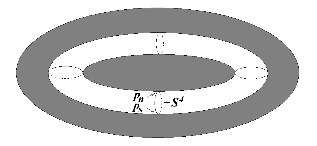
Figure 4: The bridge connecting the black annulus with the inner black disk.

Due to the new bridge, the topology is changed. This bridge connects the central black droplet with the black annulus (see Figure 4). This bridge is the $S^{3}$ fibration over the white annulus. This is a bridge connecting two different regions of the same spacetime. It has topology $S^{1}\times S^{4},$ where $S^{1}$ is the circular direction on the black and white plane. The $S^{4}$ is formed due to that a $S^{3}$ shrinks smoothly at the outer and inner edges of the white annulus, and it generates a nontrivial fourth homology class of the geometry. This bridge connects with the inner black disk along $S^{1}\times\{p_{\mathrm{n}}\}$ and with the black annulus along $S^{1}\times\{p_{\mathrm{s}}\}$, where $p_{\mathrm{n}}$ and $p_{\mathrm{s}}$ are the north pole and south pole of the $S^{4}$. The geometric property of the bridge depends on $L,M$. The emergence of this bridge structure is closely related to the entanglement between modes of the rectangular tableau state. This is reminiscent to the proposal in [5].

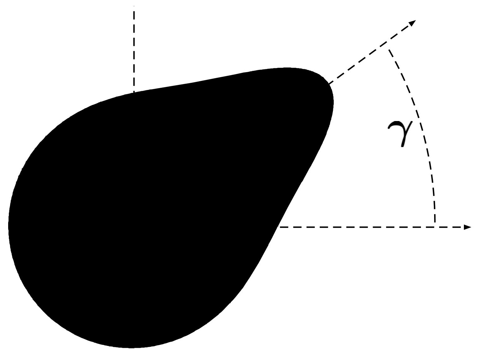
(a) Coherent state with a single bump

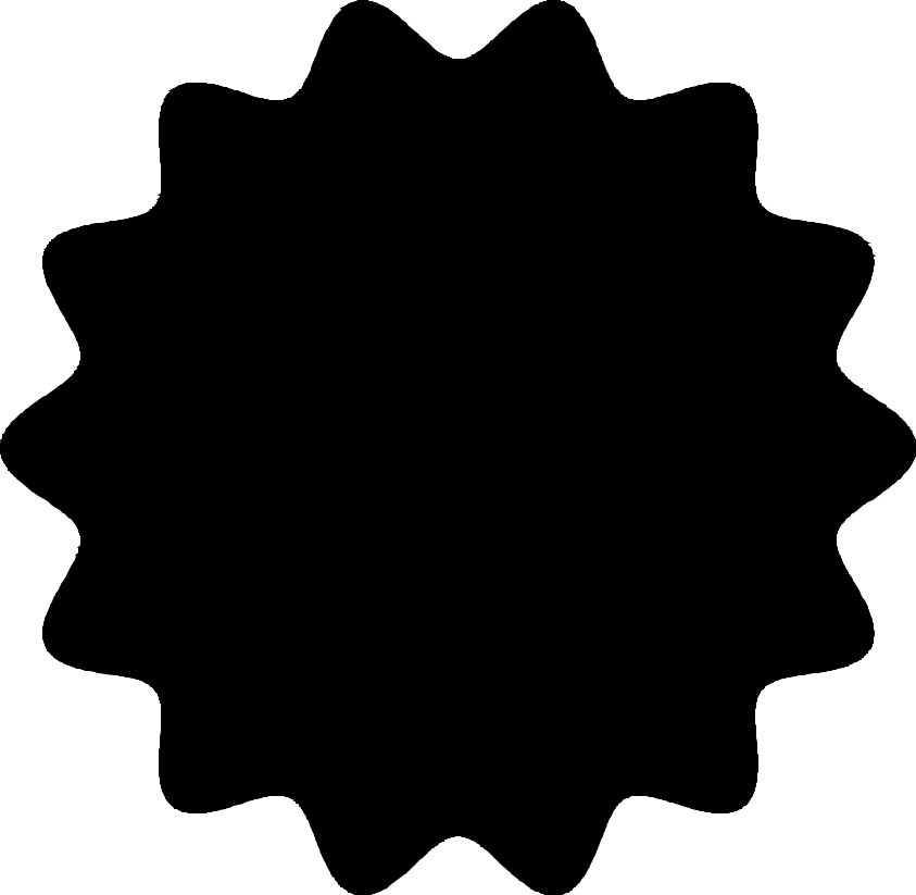
(b) Coherent state with multiple bumps that are uniformly distributed

Figure 5: Droplet picture of the bubbling geometries for coherent states. Figure (a) corresponds to a single bump at angle $\gamma$ which corresponds to the state $B_{+,x}\lvert{0}\rangle$, where $x=re^{i\gamma}$. The parameter $r\in(0,1)$ determines the height of the bump. The larger the $r$ is, the higher the bump is. And at the limit $r\to 1$, this bump becomes a Dirac delta function. Figure (b) shows $M$ bumps, where all $x_{i}$ uniformly distribute around a circle in the complex plane.

In deriving this result, we have assumed that all $r_{i}=|x_{i}|$ are equal for saturation of the bound, which is verified in Appendix B. There is also a physical interpretation to this. The physical meaning of the above inequality is to find the upper bound of the overlap of the two states $\lvert{\Box_{LM}}\rangle$ and $\prod_{i=1}^{M}B_{+,x_{i}}\lvert{0}\rangle$. The geometry corresponding to the state $\lvert{\Box_{LM}}\rangle$ is a circular black droplet surrounded by a black annulus. This geometry has an axial symmetry. On the other hand, we can look at the geometry corresponding to the state $B_{+,x}\lvert{0}\rangle$. We have a chiral field $\hat{\phi}(\theta)=\sum_{k>0}(a_{k}\exp(-ik\theta)+a_{k}^{\dagger}\exp(ik\theta))$. We can calculate the expectation value of the chiral field $\phi(\theta)=\langle\hat{\phi}(\theta)\rangle_{B_{+,x}\lvert{0}\rangle}$, which is

$$\phi(\theta) =\sum_{k=1}^{\infty}x^{k}\exp(-ik\theta)+\bar{x}^{k}\exp(ik\theta)$$

$$=2\Re(\frac{xe^{-i\theta}}{1-xe^{-i\theta}}).$$ (4.6)

The chiral field $\phi(\theta)$ can be regarded as the displacement of the geometric interface of the two regions, black and white, associated to the coherent state $B_{+,x}\lvert{0}\rangle$. Writing $x=re^{i\gamma}$, we can then draw a picture of $\phi(\theta)$, which is like a bump at angle $\gamma$ whose height is determined by $r$ (see Figure 5 (a)). For state $\prod_{i=1}^{M}B_{+,x_{i}}\lvert{0}\rangle$, with $x_{i}$ uniformly distributed around the circle, the corresponding geometry will be like $M$ bumps with the same height that uniformly distributed along the angular direction (see Figure 5 (b)). This is the state with the most possible axial symmetry. Therefore we expect that the maximum will only be obtained at this state.

5 Generalized expansion formula

We consider a generalization of the expansion formula for the Young tableau states in terms of coherent states, in integral representation. Let’s first consider $B_{+}(e^{i\theta})\lvert{0}\rangle=\sum_{n}e^{in\theta}\lvert{\triangle_{n}}\rangle$, for the single row states. We write $z=re^{i\theta}$, then $B_{+}(z)\lvert{0}\rangle=\sum_{n}z^{n}\lvert{\triangle_{n}}\rangle$. Then $\lvert{\triangle_{n}}\rangle$ can be written as

$$\lvert{\triangle_{n}}\rangle=\frac{1}{2\pi i}\oint_{\mathcal{C}}\frac{\mathrm{d}z}{z}z^{-m}B_{+}(z)\lvert{0}\rangle,$$ (5.1)

where $\mathcal{C}$ can be any path that encloses $0$.

Hence we can use Fourier transform to represent the single row state $\lvert{\triangle_{n}}\rangle$ through coherent state

$$\lvert{\triangle_{n}}\rangle=\frac{1}{2\pi}\int_{0}^{2\pi}\mathrm{d}\gamma e^{-in\gamma}B_{+,e^{i\gamma}}\lvert{0}\rangle.$$ (5.2)

We then find a generalization of this formula to any Young tableau state.

Theorem 5.1.

Let $\lambda$ be a Young tableau with $M$ rows (that is, $\lambda=(\lambda_{1},\lambda_{2},\dots,\lambda_{M})$). Then the Young tableau state $\lvert\lambda\rangle$ can be represented by coherent state $B_{+}(x_{1},\dots,x_{M})\lvert{0}\rangle$ by the following formula

$$\lvert\lambda\rangle=\frac{1}{M!(2\pi)^{M}}\int_{[0,2\pi]^{M}}\mathrm{d}\theta_{1}\dots\mathrm{d}\theta_{M}s_{\lambda}(e^{-i\theta_{1}},\dots,e^{-i\theta_{M}})\prod_{1\leq i<j\leq M}|e^{i\theta_{i}}-e^{i\theta_{j}}|^{2}B_{+}(e^{i\theta_{1}},\dots,e^{i\theta_{M}})\lvert{0}\rangle.$$ (5.3)

Proof.

Our proof of the above formula requires using a formula presented in [46]

$$\frac{1}{(2\pi)^{M}}\int_{[0,2\pi]^{M}}\mathrm{d}\theta_{1}\cdots\mathrm{d}\theta_{n}J_{\lambda}^{(\alpha)}(e^{i\theta_{1}},\dots,e^{i\theta_{M}})\overline{J_{\mu}^{(\alpha)}(e^{i\theta_{1}},\dots,e^{i\theta_{M}})}\prod_{1\leq i<j\leq M}|e^{i\theta_{i}}-e^{i\theta_{j}}|^{2/{\alpha}}$$ (5.4)

$$= \delta_{\lambda\mu}\frac{\Gamma(M/\alpha+1)}{\Gamma(1+1/\alpha)^{M}}C_{\lambda}(\alpha)\mathcal{N}_{\lambda}^{\alpha}(M)$$

where they used Jack polynomial $J_{\lambda}^{(\alpha)}$ (see Section 4.1 of Ref. [46] for details).

For $\alpha=1$, the Jack polynomial $J_{\lambda}^{(\alpha)}$ is a scalar multiple of the Schur polynomial, $J_{\lambda}^{(1)}=h(\lambda)s_{\lambda}$ where $h(\lambda)$ is the hook length product. For $\alpha=1$, the above formula becomes

$$\frac{1}{(2\pi)^{M}}\int_{[0,2\pi]^{M}}\mathrm{d}\theta_{1}\cdots\mathrm{d}\theta_{M}s_{\mu}(e^{i\theta_{1}},\dots,e^{i\theta_{M}})\overline{s_{\lambda}(e^{i\theta_{1}},\dots,e^{i\theta_{M}})}\prod_{1\leq i<j\leq M}|e^{i\theta_{i}}-e^{i\theta_{j}}|^{2}=\delta_{\lambda\mu}M!.$$ (5.5)

Since

$$B_{+}(e^{i\theta_{1}},\dots,e^{i\theta_{M}})=\sum_{\mu}s_{\mu}(e^{i\theta_{1}},\dots,e^{i\theta_{M}})\lvert\mu\rangle,$$ (5.6)

then we times $\frac{1}{(2\pi)^{M}M!}\overline{s_{\lambda}(e^{i\theta_{1}},\dots,e^{i\theta_{M}})}\prod_{1\leq i<j\leq M}|e^{i\theta_{i}}-e^{i\theta_{j}}|^{2}$ to both side of equation (5.6) and integrate all $\theta_{l}$, the left hand side is just the right hand side of (5.3), and the right hand side becomes

$$\sum_{\mu}\delta_{\lambda\mu}\lvert\mu\rangle=\lvert\lambda\rangle.$$ (5.7)

This gives us equation (5.3). ∎

For special case $\lambda=\Box_{LM}$, the above formula becomes

$$\lvert\Box_{LM}\rangle=\frac{1}{M!(2\pi)^{M}}\int_{[0,2\pi]^{M}}\mathrm{d}\theta_{1}\cdots\mathrm{d}\theta_{M}e^{-iL(\theta_{1}+\dots+\theta_{M})}\prod_{1\leq i<j\leq M}|e^{i\theta_{i}}-e^{i\theta_{j}}|^{2}B_{+}(e^{i\theta_{1}},\dots,e^{i\theta_{M}})\lvert{0}\rangle.$$ (5.8)

For special case $\lambda=(n)$, then this formula just gives our previous formula (5.2).

This is a generalized expansion formula in integral representation. The relation between this formula and $B_{+}(x_{1},x_{2},\dots)=\sum_{\lambda}s_{\lambda}\lvert\lambda\rangle$ is just like the relation between formula $\lvert{\triangle_{n}}\rangle=\frac{1}{2\pi}\int_{0}^{2\pi}\mathrm{d}\gamma e^{-in\gamma}B_{+,e^{i\gamma}}\lvert{0}\rangle$ and $B_{+}(x)\lvert{0}\rangle=\sum_{n}x^{n}\lvert{\triangle_{n}}\rangle$, where we take inverse Fourier transform of $B_{+}(x)\lvert{0}\rangle$ to get $\lvert{\triangle_{n}}\rangle$. This is some kind of generalized Fourier transform in the case of symmetric polynomial.

There is also an analogous formula for $B_{-}(-x_{1},-x_{2},\dots)$. The dual of a coherent state $B_{+}(x_{1},x_{2},\dots)$ is just $B_{-}(-x_{1},-x_{2},\dots)$. Then we just need to take the dual of the formula to give

$$\lvert\lambda^{T}\rangle=\frac{1}{M!(2\pi)^{M}}\int_{[0,2\pi]^{M}}\mathrm{d}\theta_{1}...\mathrm{d}\theta_{M}s_{\lambda}(e^{-i\theta_{1}},...,e^{-i\theta_{M}})\prod_{1\leq i<j\leq M}|e^{i\theta_{i}}-e^{i\theta_{j}}|^{2}B_{-}(-e^{i\theta_{1}},...,-e^{i\theta_{M}})\lvert{0}\rangle,$$ (5.9)

where $M$ is the number of columns of the Young tableau $\lambda^{T}$. This is easily proved in the same way as in the above proof. The equation (5.3) is dual to (5.9).

It is very interesting that the paper [46] is on Probability Theory and actually discuss Random matrix. This is not a surprise because our system also has a matrix theory description. And it’s also very interesting that some formulas given in [46] will be useful in our system.

6 Squeezed states and multi-mode entangled states from Young tableau states

Here we discuss other states that are of interest, including the two-mode squeezed states and multi-mode entangled states. In quantum information theory and quantum optics, these states naturally arise for their enormous applications. Putting these states into our setting, we find other interesting results. We compute their overlaps with the Young tableau states, and further make expansions of them in terms of Young tableau states.

Let us first consider the two-mode squeezed states

$$\lvert\mathrm{Squ}_{kk^{\prime}}\rangle=\exp\left[\mu(a_{k}^{\dagger}a_{k^{\prime}}^{\dagger}-a_{k}a_{k^{\prime}})\right]\lvert{0}\rangle.$$ (6.1)

One mode is created by $a_{k}^{\dagger}$ and belongs to the Hilbert space $\mathcal{H}_{k}$. At the same time, the other mode is created by $a_{k^{\prime}}^{\dagger}$ and belongs to the Hilbert space $\mathcal{H}_{k^{\prime}}$. For simplicity, we consider the parameter $\mu$ to be real. After using the commutation relations

$$\left[\frac{a_{k_{1}}}{\sqrt{k_{1}}},~{}\frac{a_{k_{2}}^{\dagger}}{\sqrt{k_{2}}}\right]=\delta_{k_{1}k_{2}},$$ (6.2)

we have that

$$\lvert\mathrm{Squ}_{kk^{\prime}}\rangle=\left(1-\tanh^{2}(\sqrt{kk^{\prime}}\mu)\right)^{\frac{1}{2}}\sum\limits_{l=0}^{\infty}\left(\tanh(\sqrt{kk^{\prime}}\mu)\right)^{l}\frac{1}{l!(\sqrt{kk^{\prime}})^{l}}\lvert t_{k}^{l}\rangle\otimes\lvert t_{k^{\prime}}^{l}\rangle.$$ (6.3)

We denote $q=\tanh(\sqrt{kk^{\prime}}\mu).$

We use the generating function $Z_{j}(t)=\langle\exp(iH_{j}t)\rangle_{\rvert\text{Squ}_{kk^{\prime}}\rangle}=\langle\exp(ia_{j}^{\dagger}a_{j}t)\rangle_{\rvert\text{Squ}_{kk^{\prime}}\rangle}$, where the expectation value is taken on squeezed state $\rvert\text{Squ}_{kk^{\prime}}\rangle$. For $j\neq k,k^{\prime}$, it is simple because $\rvert\text{Squ}_{kk^{\prime}}\rangle$ do not contain a $j$ mode. For $j=k$, consider

$$\exp(iH_{k}t)\rvert\text{Squ}_{kk^{\prime}}\rangle=(1-q^{2})^{\frac{1}{2}}\sum_{l=0}^{\infty}\frac{q^{l}}{l!(\sqrt{kk^{\prime}})^{l}}\exp(ilkt)\lvert t_{k}^{l}\rangle\otimes\lvert t_{k^{\prime}}^{l}\rangle.$$ (6.4)

Thus we have

$$Z_{k}(t)=\langle\exp(iH_{k}t)\rangle_{\rvert\text{Squ}_{kk^{\prime}}\rangle}=(1-q^{2})\sum_{l=0}^{\infty}q^{2l}\exp(ilkt)=\frac{1-q^{2}}{1-q^{2}\exp(ikt)}.$$ (6.5)

Likewise, for $j=k^{\prime}$, we get

$$Z_{k^{\prime}}(t)=\frac{1-q^{2}}{1-q^{2}\exp(ik^{\prime}t)}.$$ (6.6)

This is just a statement that for mode $k$ or $k^{\prime}$, the probability distribution is $p_{l}\propto q^{2l}$. This can also be shown by directly calculating the reduced density matrix through tracing.

The overlaps between the above squeezed states and the Young tableau states are hence

$$\langle\lambda\lvert\text{Squ}_{kk^{\prime}}\rangle=\left(1-q^{2}\right)^{\frac{1}{2}}\frac{q^{l}}{l!(\sqrt{kk^{\prime}})^{l}}\chi_{\lambda}(\vec{w})\rvert_{\begin{subarray}{c}w_{k}=w_{k^{\prime}}=l;\\ w_{p}=0,p\neq k,k^{\prime}\end{subarray}}.$$ (6.7)

And $\lambda\vdash l(k+k^{\prime})$.

It’s easy to see that the above squeezed states have the inner products

$$\langle\mathrm{Squ}_{k_{1}k_{2}}\rvert\mathrm{Squ}_{k_{3}k_{4}}\rangle=\delta_{k_{1}k_{3}}\delta_{k_{2}k_{4}}+\delta_{k_{1}k_{4}}\delta_{k_{2}k_{3}}.$$ (6.8)

As the Young tableau states are orthonormal [10], the squeezed states are the linear combinations of the Young tableau states as

$$\rvert\mathrm{Squ}_{kk^{\prime}}\rangle=\left(1-q^{2}\right)^{\frac{1}{2}}\sum_{l=0}^{\infty}\sum_{\lambda\vdash l(k+k^{\prime})}\left(\frac{q^{l}}{l!(\sqrt{kk^{\prime}})^{l}}\chi_{\lambda}(\vec{w})\rvert_{\begin{subarray}{c}w_{k}=w_{k^{\prime}}=l;\\ w_{p}=0,p\neq k,k^{\prime}\end{subarray}}\right)\lvert\lambda\rangle.$$ (6.9)

Taking a limit $\sqrt{kk^{\prime}}\mu\rightarrow\infty$, or equivalently $q\rightarrow 1$, the above two-mode squeezed states become maximally entangled states, or EPR states $\lvert\mathrm{EPR}\rangle=\lim_{\sqrt{kk^{\prime}}\mu\rightarrow\infty}\lvert\mathrm{Squ}_{kk^{\prime}}\rangle$, which are

$$\lvert\mathrm{EPR}\rangle=\mathcal{N}^{-\frac{1}{2}}\sum\limits_{l=0}^{\infty}\frac{1}{l!(\sqrt{kk^{\prime}})^{l}}\lvert t_{k}^{l}\rangle\otimes\lvert t_{k^{\prime}}^{l}\rangle,$$ (6.10)

where $\mathcal{N}^{-\frac{1}{2}}$ is a normalization factor. The normalization factor can be understood as follows. One can take an infinitesimal positive cutoff $\epsilon\rightarrow 0$, such that $1-q=\epsilon$ and $\mathcal{N}=\frac{1}{2\epsilon}$. The squeezed state $\lvert\mathrm{Squ}_{kk^{\prime}}\rangle$ with $q$ close to 1, is a good approximation to the EPR state. These are the entangled states in $\mathcal{H}_{k}\otimes\mathcal{H}_{k^{\prime}}$, in which the states $\lvert l\rangle_{k}=\frac{1}{\sqrt{l!k^{l}}}\lvert t_{k}^{l}\rangle$ in mode $k$, are entangled with the states $\lvert l\rangle_{k^{\prime}}=\frac{1}{\sqrt{l!(k^{\prime})^{l}}}\lvert t_{k^{\prime}}^{l}\rangle$ in mode $k^{\prime}$. Consider mode $k$ as a IR mode with $k$ very small, and consider mode $k^{\prime}$ as a UV mode with $k^{\prime}$ very big. Then this state is an entangled state between a IR mode and a UV mode. Integrating out the UV mode, gives rise to a reduced density matrix of the IR mode.

The EPR states and the Young tableau states have overlaps

$$\langle\lambda\rvert\mathrm{EPR}\rangle=\mathcal{N}^{-\frac{1}{2}}\frac{1}{l!(\sqrt{kk^{\prime}})^{l}}\chi_{\lambda}(\vec{w})\rvert_{\begin{subarray}{c}w_{k}=w_{k^{\prime}}=l;\\ w_{p}=0,p\neq k,k^{\prime}\end{subarray}}.$$ (6.11)

Thus the EPR states can be written as the linear combinations of the Young tableau states as

$$\rvert\mathrm{EPR}\rangle=\mathcal{N}^{-\frac{1}{2}}\sum_{l=0}^{\infty}\sum_{\lambda\vdash l(k+k^{\prime})}\left(\frac{1}{l!(\sqrt{kk^{\prime}})^{l}}\chi_{\lambda}(\vec{w})\rvert_{\begin{subarray}{c}w_{k}=w_{k^{\prime}}=l;\\ w_{p}=0,p\neq k,k^{\prime}\end{subarray}}\right)\lvert\lambda\rangle.$$ (6.12)

Consider the state

$$\sqrt{1-q^{2}}(\sum_{l=0}^{\infty}q^{l}\lvert l\rangle_{k}\lvert l\rangle_{k^{\prime}}\lvert l\rangle_{k^{\prime\prime}})=\sqrt{1-q^{2}}(\sum_{l=0}^{\infty}q^{l}\frac{1}{\sqrt{(l!)^{3}(kk^{\prime}k^{\prime\prime})^{l}}}\lvert{t_{k}^{l}}\rangle\lvert{t_{k^{\prime}}^{l}}\rangle\lvert{t_{k^{\prime\prime}}^{l}}\rangle),$$ (6.13)

while the GHZ state corresponds to the $q\rightarrow 1$ limit. In our system, a three mode entangled GHZ state, should generalize the above state as

$$\lvert\mathrm{GHZ}\rangle=\tilde{\mathcal{N}}^{-\frac{1}{2}}(\sum_{l=0}^{\infty}\lvert l\rangle_{k}\lvert l\rangle_{k^{\prime}}\lvert l\rangle_{k^{\prime\prime}}).$$ (6.14)

This is an entangled state in $\mathcal{H}_{k}\otimes\mathcal{H}_{k^{\prime}}\otimes\mathcal{H}_{k^{\prime\prime}}$. Then we trace out any two modes, and this gives a density matrix

$$\hat{\rho}=(1-q^{2})\sum_{l=0}^{\infty}q^{2l}\lvert l\rangle_{k}\langle{l}\rvert_{k}~{}.$$ (6.15)

The entropy for this density matrix is $s=-(\log(1-q^{2})+\frac{2q^{2}\log(q)}{1-q^{2}})$, and taking $q\rightarrow 1$ limit gives $s\rightarrow\infty$.

The GHZ states and the Young tableau states have overlaps

$$\langle\lambda\rvert\mathrm{GHZ}\rangle=\tilde{\mathcal{N}}^{-\frac{1}{2}}\frac{1}{\sqrt{(l!)^{3}(kk^{\prime}k^{\prime\prime})^{l}}}\chi_{\lambda}(\vec{w})\rvert_{\begin{subarray}{c}w_{k}=w_{k^{\prime}}=w_{k^{\prime\prime}}=l;\\ w_{p}=0,p\neq k,k^{\prime},k^{\prime\prime}\end{subarray}}.$$ (6.16)

The GHZ states can thus be written as the linear combinations of the Young tableau states as

$$\rvert\mathrm{GHZ}\rangle=\tilde{\mathcal{N}}^{-\frac{1}{2}}\sum_{l=0}^{\infty}\sum_{\lambda\vdash l(k+k^{\prime}+k^{\prime\prime})}\left(\frac{1}{\sqrt{(l!)^{3}(kk^{\prime}k^{\prime\prime})^{l}}}\chi_{\lambda}(\vec{w})\rvert_{\begin{subarray}{c}w_{k}=w_{k^{\prime}}=w_{k^{\prime\prime}}=l;\\ w_{p}=0,p\neq k,k^{\prime},k^{\prime\prime}\end{subarray}}\right)\lvert\lambda\rangle$$ (6.17)

and $\lambda\vdash l(k+k^{\prime}+k^{\prime\prime})$.

It is easy to generalize the state in (6.14), (6.17) to a $m$-mode GHZ state with $m>3$,

$$\lvert\mathrm{GHZ}\rangle_{m} = \tilde{\mathcal{N}}_{m}^{-\frac{1}{2}}(\sum_{l=0}^{\infty}\lvert l\rangle_{k_{1}}\lvert l\rangle_{k_{2}}\dots\lvert l\rangle_{k_{m}})$$

$$= \tilde{\mathcal{N}}_{m}^{-\frac{1}{2}}\sum_{l=0}^{\infty}\sum_{\lambda\vdash l(k_{1}+k_{2}+\dots+k_{m})}\left(\frac{1}{\sqrt{(l!)^{m}(k_{1}k_{2}\dots k_{m})^{l}}}\chi_{\lambda}(\vec{w})\rvert_{\begin{subarray}{c}w_{k_{1}}=w_{k_{2}}=\dots=w_{k_{m}}=l;\\ w_{p}=0,p\neq k_{1},k_{2},\dots,k_{m}\end{subarray}}\right)\lvert\lambda\rangle.$$

We can also calculate the inner product $\langle\text{Squ}_{kk^{\prime}}\lvert B_{+}(x_{1},\dots)\rvert 0\rangle$, which is just the symmetric polynomial associated with $\rvert\text{Squ}_{kk^{\prime}}\rangle$. We get the inner product

$$\langle\text{Squ}_{kk^{\prime}}\lvert B_{+}(x_{1},x_{2},\dots)\rvert 0\rangle=(1-q^{2})^{\frac{1}{2}}\sum_{l=0}^{\infty}\frac{q^{l}}{l!(\sqrt{kk^{\prime}})^{l}}p_{k}^{l}p_{k^{\prime}}^{l}=(1-q^{2})^{\frac{1}{2}}\exp(\frac{q}{\sqrt{kk^{\prime}}}p_{k}p_{k^{\prime}}),$$ (6.19)

where $p_{k}=x_{1}^{k}+x_{2}^{k}+\dots$ , and $p_{k^{\prime}}=x_{1}^{k^{\prime}}+x_{2}^{k^{\prime}}+\dots$. Hence,

$$\langle\text{Squ}_{kk^{\prime}}\lvert B_{+}(x_{1},x_{2},\dots)\rvert 0\rangle=(1-q^{2})^{\frac{1}{2}}\exp(\frac{q}{\sqrt{kk^{\prime}}}(x_{1}^{k}+x_{2}^{k}+\dots)(x_{1}^{k^{\prime}}+x_{2}^{k^{\prime}}+\dots)).$$ (6.20)

This result is just a special case of the fact that the overlap of any state with $B_{+}(x_{1},\dots)\rvert 0\rangle$ is the symmetric polynomial associated with that state. See proposition 3.2.

Consider the field

$$\hat{\phi}(\theta)=\sum_{m>0}a_{m}\exp(-im\theta)+a_{m}^{\dagger}\exp(im\theta).$$ (6.21)

First the expectation value of this field on the above squeezed states is zero, $\langle\hat{\phi}(\theta)\rangle=0$. Then we compute the variance $\langle$Squ${}_{kk^{\prime}}\lvert:\hat{\phi}^{2}(\theta):\rvert$Squ${}_{kk^{\prime}}\rangle$, where $:\hat{\phi}^{2}(\theta):$ is the normal ordering of $\hat{\phi}^{2}(\theta)$. The variance is

$$\langle\text{Squ}_{kk^{\prime}}\lvert:\hat{\phi}^{2}(\theta):\rvert\text{Squ}_{kk^{\prime}}\rangle=\frac{2q}{(1-q^{2})}(q(k+k^{\prime})+2\sqrt{kk^{\prime}}\cos((k+k^{\prime})\theta)).$$ (6.22)

The detailed derivation of the above expression is in Appendix C. This result also reveals that the squeezed state is not rotationally symmetric. We also calculate other quantities like $\langle{\hat{N}}_{j}\rangle=\langle a_{j}^{\dagger}a_{j}\rangle$ and $\langle a_{m}^{\dagger}a_{j}\rangle,$

$$\langle a_{m}^{\dagger}a_{j}\rangle=\begin{cases}\frac{q^{2}}{(1-q^{2})}k&~{}~{}~{}m=j=k\\ \frac{q^{2}}{(1-q^{2})}k^{\prime}&~{}~{}~{}m=j=k^{\prime}\\ 0&~{}~{}~{}\text{others}\end{cases}.$$ (6.23)

The squeezed state is interesting that it tells us that we can create a EPR pair by squeezing the vacuum. They and the multi-mode entangled states can be expanded by Young tableau states in the setup here and are very interesting states in gauge/gravity correspondence. For discussions of squeezed states in quantum information theory and quantum optics, see for example [21, 47, 48, 49]. GHZ states are also very important in quantum information theory [50].

7 Discussion

We computed a momentum space version of the entanglement spectrum and entanglement entropy of Young tableau states and one-point functions on Young tableau states. The Young tableau states are not direct product states, and they have non-zero entanglement between modes. The entanglement spectrum and entanglement entropy of general Young tableau states are obtained. We have also computed the generating functions for one-point functions on Young tableau states. These physical quantities in the field theory side are used to measure the topology of the dual spacetime geometries, such as the number of annuli in the geometries and the existence of bridge structures which connect different regions of the same spacetime. Our results indicate that the emergence of the bridge structure is closely related to the entanglement between modes of the Young tableau states.

On one hand, we can expand a coherent state above the vacuum as the linear combination of Young tableau states through our explicit expression for the inner products between coherent states and general Young tableau states. This is an analog of Fourier transform. On the other hand, the Young tableau states can be obtained by superposition of coherent states, and we further presented an integral formula as an inverse transform. Thus we get two sets of formulas, one is to express coherent states by Young tableau states and the second is to express Young tableau states by coherent states, and the relation between these two sets of formulas is an analogy to the Fourier transform and its inverse transform. These formulas are also of mathematical interest. Form a physical point of view, we are particularly interested in expressing the rectangular Young tableau state by coherent states, since the superposed geometry (see Figure 1 (a)) has a different topology than the original geometries (see Figure 1 (b, c)) participating in the superposition. At the same time, the bridge structure emerged after the topology change, and this is related to the entanglement between modes of the Young tableau states. We can then generalize the case of rectangular Young tableau states to other Young tableau states. This further implies that we can superpose topology trivial states to get states with complicated geometry and topology in the gravity side.

One important feature of our system is that these states with different topologies live in the same Hilbert space, hence one can concretely study the transition amplitudes between different states from the dual quantum mechanical system. We analyzed the overlaps between Young tableau states and coherent states, and carried out in detail for the rectangular tableaux, corresponding to the geometries with one black annulus. As shown in Section 4, we have a refined bound for the overlap between coherent states and a rectangular Young tableau state. The overlap between two states differed by this topology change is exponentially suppressed. Hence to produce a topologically distinct geometry by superposing coherent states dual to geometries with a trivial topology, it requires at least an exponentially large number of states in the superposition. This is essentially a non-perturbative effect in quantum gravity. It is further found that the norm squared of the overlaps is bounded above by the inverse powers of the exponential of the entanglement entropies. Our results put into firmer footing the insights and observations in [11, 33, 34]. Incidentally, we also find that the overlap of any state with the coherent state defined in Section 3, is a symmetric function associated with that state. This greatly generalized the results in [11]. And it provides us an approach to analyze the overlap between a coherent state and an arbitrary state with more complicated topology, like those with more white rings, which correspond to Young tableaux with more long edges. Since one can understand the norm squared of the overlap as the transition probability between a topology trivial state and a state with a distinct topology, it would be valuable to explore the relation between the transition probabilities and the geometric and topological properties of the states. Also, our analysis related the characters of the symmetric groups [23, 24] to the topologies of the bubbling geometries. We hope that more physical intuition will give further mathematical insights into related subjects.

Here, these exponentially large number of states participating in the superposition have caused the topology change. On the other hand, the situations with a small number of states participating in the superposition can be different from the situations with an exponentially large number of states in the superposition. The former cases would imply relatively bigger overlaps between individual states. Their differences are also pointed out in [51] and [52] in closely related discussions.

The theorem in Section 2 and a proposition in Section 3 are analogous to giant/dual-giant duality. These are dualities between giant gravitons wrapping AdS directions and dual giant gravitons wrapping internal directions. They have also appeared in other context, see for example [53, 54, 55, 56, 57, 58] in two-point and three-point functions of giant gravitons. Moreover, bearing the different aspects to look at our system in mind, this giant/dual-giant duality can have interpretations in other ways. In the droplet picture, this duality is a particle/hole duality. Since each state is associated with a symmetric function, this duality can be explained in terms of an involution on the ring of symmetric functions.

Topology change in bubbling geometries were also discussed in [59, 60]. Other aspects of describing topology on the gravity side from the field theory side have been put forward, in [61, 62, 63] by using correlation functions for the states dual to strings on bubbling geometries, in [13] by using correlation functions for the states undergoing topology change, and in [12] by using probability theory on the graphs of representations [64].

To sum over different topologies and geometries are important issues in quantum gravitational theories, see for example [11, 6, 65, 66]. Various other similar geometries in the context of string theory and quantum gravity have been analyzed, see for example [67$-$76, 17] and their related discussions. Our approach may also be related to fuzzball proposal [20] and to 2d Yang-Mills [77]. It would also be good to understand in more detail the relation to the scenarios of building spacetime geometries, as proposed in for example [5, 78, 4].

Two mode squeezed states and multi-mode entangled states are also discussed, and the two mode maximally entangled state, the EPR state, is a particular limit of the squeezed state. They have similarities with those states appeared in quantum optics and quantum information theory [21, 47, 48, 49]. However, our setup provides another framework to explore their properties. By computing their overlaps with Young tableau states, we expanded them as linear combinations of Young tableau states. Maybe we can consider the EPR state in Section 6 as similar to creating a squeezed state string connecting between mode $k$ and $k^{\prime}$. We think that it would be similar to the situations in the ER=EPR proposal [78]. This proposal [78] has related the geometry side [79] to the side of quantum mechanics system [80] and conjectured that entangled black holes are connected by worm hole. It may be interesting to understand more the relations to this proposal for the squeezed states and EPR states discussed in Section 6.

The approach here describes measuring the topologies of spacetime from the dual field theory side, and therefore will be interesting and useful for understanding the emergence of spacetime structures, see for example [4, 5, 6, 7]. These geometries are very explicit and they serve as a good laboratory to perform quantitative calculations and predictions. Moreover, the system is UV finite, since it has UV completion in string theory. Various other discussions on entanglement entropies with bubbling geometries are recently in for example [81] and it would be interesting to see the relation to the discussions here.

The entanglement entropies here arise after partial tracing out other momentum modes living in the momentum space version of the Hilbert space decomposition. The subsystem in this case, is a region in the momentum space. Consider high energy UV modes entangled with low energy IR modes. Then tracing out the high energy modes gives a reduced density matrix for the low energy modes. Hence in these cases, physics at low energy can still be sensitive to the details of the physics at high energy. This momentum space version of the entanglement entropy is similar but slightly different from the usual real space version of the entanglement entropy, where the real space version of the Hilbert space decomposition is used and the subsystems are domains in real space. The two are related by a different decomposition of the Hilbert space.

Appendix A Overlap of coherent states and Young tableau states

The norm-squared $\|B_{+,x_{1}}B_{+,x_{2}}\lvert{0}\rangle\|^{2}$ was computed in Eq. (4.44) of [11]. We can generalize this formula to the inner products of arbitrarily many $B_{+,x_{i}}$, and we have the following result

$$\langle{0}\rvert(\prod_{i}B_{+,y_{i}}^{\dagger})(\prod_{i}B_{+,x_{i}})\lvert{0}\rangle=\prod_{i,j}\frac{1}{1-x_{i}\bar{y}_{j}}.$$ (A.1)

Proof.

Write

$$\prod_{i}B_{+,x_{i}}\lvert{0}\rangle=\sum_{\lambda}s_{\lambda}(x_{1},x_{2},\dots)\lvert{\lambda}\rangle,$$ (A.2)

then insert it in the above formula

$$\langle{0}\rvert(\prod_{i}B_{+,y_{i}}^{\dagger})(\prod_{i}B_{+,x_{i}})\lvert{0}\rangle =\langle{0}\rvert(\prod_{i}B_{+,y_{i}}^{\dagger})\sum_{\lambda}s_{\lambda}(x_{1},x_{2},\dots)\lvert{\lambda}\rangle$$

$$=\sum_{\lambda}s_{\lambda}(x_{1},x_{2},\dots)\langle{0}\rvert(\prod_{i}B_{+,y_{i}}^{\dagger})\lvert{\lambda}\rangle$$

$$=\sum_{\lambda}s_{\lambda}(x_{1},x_{2},\dots)s_{\lambda}(\bar{y}_{1},\bar{y}_{2},\dots)$$

$$=\prod_{i,j}\frac{1}{1-x_{i}\bar{y}_{j}}.$$ (A.3)

In the last line, we used the Cauchy identity. ∎

Consider the case that we only have one variable $x_{1}$ and $y_{1}=x_{1}$, then the above formula gives Eq. (4.6) in [11], and for two variables $x_{1}=y_{1},\;x_{2}=y_{2}$, our formula gives Eq. (4.44) in [11].

It is easy to see the norm of the $\prod_{i}B_{+,x_{i}}\lvert{0}\rangle$ from (A.1), when identifying $y_{i}$ with $x_{i}$, hence

$$\parallel\prod_{i}B_{+,x_{i}}\lvert{0}\rangle\parallel^{2}=\prod_{i,j}\frac{1}{1-x_{i}\bar{x}_{j}}.$$ (A.4)

There is a dual version of the above formula for operators $B_{-,x_{i}}$, which gives the same result as above

$$\langle{0}\rvert(\prod_{i}B_{-,y_{i}}^{\dagger})(\prod_{i}B_{-,x_{i}})\lvert{0}\rangle=\prod_{i,j}\frac{1}{1-x_{i}\bar{y}_{j}}.$$ (A.5)

Proof.

According to Proposition 3.16,

$$\langle{\lambda^{T}}\rvert\prod_{i}B_{-,-x_{i}}\lvert{0}\rangle=s_{\lambda},$$ (A.6)

therefore

$$\prod_{i}B_{-,x_{i}}\lvert{0}\rangle=\sum_{\lambda}s_{\lambda}(-x_{1},-x_{2},\dots)\lvert{\lambda^{T}}\rangle.$$ (A.7)

Inserting this into the inner product,

$$\langle{0}\rvert(\prod_{i}B_{-,y_{i}}^{\dagger})(\prod_{i}B_{-,x_{i}})\lvert{0}\rangle =\langle{0}\rvert(\prod_{i}B_{-,y_{i}}^{\dagger})\sum_{\lambda}s_{\lambda}(-x_{1},-x_{2},\dots)\lvert{\lambda^{T}}\rangle$$

$$=\sum_{\lambda}s_{\lambda}(-x_{1},-x_{2},\dots)\langle{0}\rvert(\prod_{i}B_{-,y_{i}}^{\dagger})\lvert{\lambda^{T}}\rangle$$

$$=\sum_{\lambda}s_{\lambda}(-x_{1},-x_{2},\dots)s_{\lambda}(-\bar{y}_{1},-\bar{y_{2}},\dots)$$

$$=\prod_{i,j}\frac{1}{1-x_{i}\bar{y}_{j}}.$$ (A.8)

∎

There is also a formula for inner product of $B_{+}$ with $B_{-}$, which is as follows

$$\langle{0}\rvert(\prod_{i}B_{-,y_{i}}^{\dagger})(\prod_{i}B_{+,x_{i}})\lvert{0}\rangle=\prod_{i,j}(1-x_{i}\bar{y}_{j}).$$ (A.9)

Proof.

$$\langle{0}\rvert(\prod_{i}B_{-,y_{i}}^{\dagger})(\prod_{i}B_{+,x_{i}})\lvert{0}\rangle =\langle{0}\rvert(\prod_{i}B_{-,y_{i}}^{\dagger})\sum_{\lambda}s_{\lambda}(x_{1},x_{2},\dots)\lvert{\lambda}\rangle$$

$$=\sum_{\lambda}s_{\lambda}(x_{1},x_{2},\dots)\langle{0}\rvert(\prod_{i}B_{-,y_{i}}^{\dagger})\lvert{\lambda}\rangle$$

$$=\sum_{\lambda}s_{\lambda}(x_{1},x_{2},\dots)s_{\lambda^{T}}(-\bar{y}_{1},-\bar{y}_{2},\dots)$$

$$=\prod_{i,j}(1-x_{i}\bar{y}_{j}).$$ (A.10)

∎

These formulas also provide the normalizations of the two-point functions for coherent states.

Appendix B Bound of overlap

As described in Section 4, we will analyze the function

$$f(x_{1},x_{2},\dots,x_{M}):=\frac{|\langle{\lambda}\rvert\prod_{i=1}^{M}B_{+,x_{i}}\lvert{0}\rangle|^{2}}{\|\prod_{i=1}^{M}B_{+,x_{i}}\lvert{0}\rangle\|^{2}}.$$ (B.1)

We consider the case with the ${\Box_{LM}}$ state which corresponds to $n_{\mathrm{anti-edge}}=1$.

Proposition B.1.

For a rectangular Young tableau with $M$ rows and $L$ columns, denoted by ${\Box_{LM}}$, and for coherent states $\prod_{i=1}^{M}B_{+,x_{i}}\lvert{0}\rangle$ with arbitrary $\{x_{i}\}$, the supremum of their normalized inner products is given by

$$\sup_{\{x_{i}\}}\left|\frac{\langle{\Box_{LM}}\rvert\prod_{i=1}^{M}B_{+,x_{i}}\lvert{0}\rangle}{\|\prod_{i=1}^{M}B_{+,x_{i}}\lvert{0}\rangle\|}\right|^{2}=(\frac{M}{L+M})^{M}(\frac{L}{L+M})^{L}.$$ (B.2)

Proof.

Writing $x_{i}=r_{i}e^{\theta_{i}}$, and inserting them into the above formula we have $f=f_{1}f_{2}=\prod_{i,j}(1-r_{i}r_{j}e^{i(\theta_{i}-\theta_{j})})\times(\prod_{i=1}^{M}r_{i}^{2})^{L}$, we can then write the first term as

$$f_{1} :=\prod_{i,j}(1-r_{i}r_{j}e^{i(\theta_{i}-\theta_{j})})$$

$$=\prod_{i}(1-r_{i}^{2})\prod_{1\leq i<j\leq M}(1-2r_{i}r_{j}\cos(\theta_{i}-\theta_{j})+r_{i}^{2}r_{j}^{2}).$$ (B.3)

Also we write the second term $f_{2}:=(\prod_{i=1}^{M}r_{i}^{2})^{L}$.

Note that the whole expression is symmetric under permutation of $r_{i},r_{j}$. Because of the axial symmetry of the Young tableau states, the distribution must be uniform along the angular direction, otherwise it will not correspond to axial symmetry. Therefore, if the maximum is unique, then it must be at $r_{i}=r,\;\forall i$. This assumption needs to be verified, and later we will verify this. Note also that the whole expression is invariant under $\theta_{i}\rightarrow\theta_{i}+\Delta\theta$, therefore we are free to choose $\theta_{1}=0$. Under the assumption that $r_{i}=r$, the expression can be simplified as

$$f=(1-r^{2})^{M}\prod_{1\leq i<j\leq M}(1-2r^{2}\cos(\theta_{i}-\theta_{j})+r^{4})\times r^{2LM}.$$ (B.4)

First consider the derivative with respect to $\theta_{l}$, $\frac{\partial\log f}{\partial\theta_{l}}$, we get

$$\frac{\partial\log f}{\partial\theta_{l}}=\sum_{j=1}^{M}\frac{2r^{2}\sin(\theta_{l}-\theta_{i})}{1-2r^{2}\cos(\theta_{l}-\theta_{i})+r^{4}}=0.$$ (B.5)

Solution to this equation is $\theta_{l}\equiv 0$ or $\theta_{l}=\frac{2\pi(l-1)}{M}$. For the first possibility, $\theta_{l}\equiv 0$. Because in this case, $f_{1}=\prod_{i,j}(1-r_{i}r_{j})$, every factor is smaller than 1, this cannot be a maximum. So we are left with the second solution $\theta_{l}=\frac{2\pi(l-1)}{M}$.

Then we consider determining $r$ that maximizes $f$. Consider the derivative $\frac{\partial\log f}{\partial r}$, we have

$$\frac{\partial\log f}{\partial r}=\frac{2LM}{r}-\frac{2rM}{1-r^{2}}-4r\sum_{k=1}^{\infty}r^{2k-2}\sum_{1\leq l<j\leq M}\Re\left(e^{i\frac{2\pi k(j-l)}{M}}\right).$$ (B.6)

Then if $k\equiv 0\mod M$, then $\sum_{1\leq l<j\leq M}\Re\left(e^{i\frac{2\pi k(j-l)}{M}}\right)=\frac{M(M-1)}{2}$. If $k\neq 0\mod M$, $\sum_{1\leq l<j\leq M}\Re\left(e^{i\frac{2\pi k(j-l)}{M}}\right)=-\frac{M}{2}$. Therefore we have

$$\frac{\partial\log f}{\partial r}=\frac{2LM}{r}-\frac{2M^{2}r^{2M-1}}{1-r^{2M}}=0.$$ (B.7)

Then $r_{0}=(\frac{L}{L+M})^{\frac{1}{2M}}$ solves this. Therefore a maximum will be obtained at $\theta_{l}=\frac{2\pi(l-1)}{M}$, $r_{l}=r_{0}=(\frac{L}{L+M})^{\frac{1}{2M}}$. This configuration is very interesting, it means that $x_{i}$ is uniformly distributed at the circle $r=r_{0}$.

Now evaluate $f$ at this point

$$f=f_{1}f_{2}=\prod_{i,j}(1-r_{0}^{2}e^{i(\theta_{i}-\theta_{j})})\times r_{0}^{2LM},$$ (B.8)

in which $f_{2}=r_{0}^{2LM}$. Observe that for any fixed $i\in\mathbb{Z}$, when $j$ runs through $1,2,\dots,M$, $\;i-j\mod M$ will also run through $1,2\dots,M$. Therefore $e^{i\frac{2\pi(i-j)}{M}}$ will run through $e^{i\frac{2\pi}{M}},e^{i\frac{2\pi\times 2}{M}},\dots,e^{i\frac{2\pi M}{M}}$. Define a set $\Theta=\{\frac{2\pi l}{M}|l=1,2,\dots,M\}$. Then $f_{1}$ can be written as

$$f_{1}=(\prod_{\phi\in\Theta}(1-r_{0}^{2}e^{i\phi}))^{M}=\exp(M\sum_{k=1}^{\infty}(-\sum_{\phi\in\Theta}\frac{r_{0}^{2k}e^{ik\phi}}{k})).$$ (B.9)

When $k\neq 0\mod M$, when $l$ runs through $1,2,\dots,M$, $kl\mod M$ also run through $1,2,\dots,M$, therefore $\sum_{\phi\in\Theta}e^{ik\phi}=0$ for $k\neq 0\mod M$. When $k\equiv 0\mod M$, $e^{ik\phi}=1$, and $\sum_{\phi\in\Theta}e^{ik\phi}=M$. Therefore the above expression will be

$$f_{1}=\exp(M\sum_{k=1}^{\infty}(-M\frac{r_{0}^{2kM}}{kM}))=(1-r_{0}^{2M})^{M}.$$ (B.10)

Then we maximize $f$ with respect to $r_{0}$.

And the final result is

$$\sup f=(\frac{M}{L+M})^{M}(\frac{L}{L+M})^{L}.$$ (B.11)

However we can’t just conclude that the state with most overlap is obtained at $x_{l}$ uniformly distributed around one circle in the complex plane. It is possible that $x_{l}$ can uniformly distribute around two or more circles but the angular positions coincide. But we can exclude this possibility by doing computation. Let’s compare the situations that $x_{l}$ uniformly distributed around one circle and two circles. For $x_{l}$ distributed around two circles write $M=2M^{\prime}$, $x_{l}=re^{i\frac{2\pi l}{M^{\prime}}}$ for $l=1,\dots,M^{\prime}$ and $x_{l}=Re^{i\frac{2\pi l}{M^{\prime}}}$ for $l=M^{\prime}+1,\dots,2M^{\prime}=M$. In this case, the norm squared of the overlap will be less than

$$(1-r^{2M^{\prime}})^{M^{\prime}}(1-R^{2M^{\prime}})^{M^{\prime}}(r^{M^{\prime}}R^{M^{\prime}})^{2L}$$

$$=(1-r^{2M^{\prime}})^{M^{\prime}}r^{2M^{\prime}L}(1-R^{2M^{\prime}})^{M^{\prime}}R^{2M^{\prime}L}$$

$$\leq((\frac{M^{\prime}}{L+M^{\prime}})^{M^{\prime}}(\frac{L}{L+M^{\prime}})^{L})^{2}=(\frac{M}{2L+M})^{M}(\frac{2L}{2L+M})^{2L}.$$ (B.12)

And we have inequality

$$(\frac{M}{2L+M})^{M}(\frac{2L}{2L+M})^{2L}<(\frac{M}{L+M})^{M}(\frac{L}{L+M})^{L}.$$ (B.13)

Similar calculation can also be done for other situations like distribution around three or more circles, and we have verified that all these situations have similar behavior as in the above case (B.12) and (B.13). The corresponding value is always smaller than the case for $x_{l}$ distribute uniformly around one circle. Hence, in conclusion, (B.11) is a global maximum. ∎

This is the most strict upper bound, in the sense that there is a state that can actually saturate this upper bound. We can consider the behavior of this upper bound at both large $L$ and large $M$, and the above formula (B.11) gives rise to

$$\sup f\leq f_{\text{bound}}=2^{-(L+M)},$$ (B.14)

where $f_{\text{bound}}$ denotes an upper bound of $f~{}$that is not necessarily a supremum.

This upper bound has significance in the superposition of coherent states to form a rectangular Young tableau state. The number of coherent states participating in the superposition has consequently a lower bound. On one hand, there are a large amount of states participating in the superposition. On the other hand, the individual overlap is very small. This is reminiscent to the observation in [11].

Appendix C Chiral field and its variances on squeezed states

Consider the field

$$\hat{\phi}(\theta)=\sum_{m>0}a_{m}\exp(-im\theta)+a_{m}^{\dagger}\exp(im\theta).$$ (C.1)

Now we compute the variance $\langle$Squ${}_{kk^{\prime}}\lvert:\hat{\phi}^{2}(\theta):\rvert$Squ${}_{kk^{\prime}}\rangle$, where $:\hat{\phi}^{2}(\theta):$ is the normal ordering of $\hat{\phi}^{2}(\theta)$. First

$$:\hat{\phi}^{2}(\theta):=\sum_{j,m>0}(a_{m}a_{j}\exp(-i(m+j)\theta)+h.c.)+\sum_{j,m>0}(a_{m}^{\dagger}a_{j}\exp(i(m-j)\theta)+h.c.).$$ (C.2)

This gives

$$\langle\text{Squ}_{kk^{\prime}}\lvert:\hat{\phi}^{2}(\theta):\rvert\text{Squ}_{kk^{\prime}}\rangle$$

$$=2\Re\left(2\langle\text{Squ}_{kk^{\prime}}\lvert a_{k}a_{k^{\prime}}\exp(-i(k+k^{\prime})\theta)\rvert\text{Squ}_{kk^{\prime}}\rangle+\sum_{j,m>0}\langle\text{Squ}_{kk^{\prime}}\lvert a_{m}^{\dagger}a_{j}\exp(i(m-j)\theta)\rvert\text{Squ}_{kk^{\prime}}\rangle\right).$$

While the first term can be computed to be

$$4\Re\left(\langle\text{Squ}_{kk^{\prime}}\lvert a_{k}a_{k^{\prime}}\exp(-i(k+k^{\prime})\theta)\rvert\text{Squ}_{kk^{\prime}}\rangle\right)$$

$$=4(1-q^{2})\Re\left(\exp(-i(k+k^{\prime})\theta)\sum_{l}(\frac{q}{\sqrt{kk^{\prime}}})^{l}\frac{1}{l!}(\frac{q}{\sqrt{kk^{\prime}}})^{l+1}\frac{kk^{\prime}(l+1)^{2}}{(l+1)!}(kk^{\prime})^{l}l!^{2}\right)$$

$$=4(1-q^{2})\cos((k+k^{\prime})\theta)\left(\sum_{l}q^{2l+1}\sqrt{kk^{\prime}}(l+1)\right)$$

$$=\frac{4q}{(1-q^{2})}\sqrt{kk^{\prime}}\cos((k+k^{\prime})\theta).$$ (C.4)

The second term is

$$2\Re\left(\sum_{j,m>0}\langle\text{Squ}_{kk^{\prime}}\lvert a_{m}^{\dagger}a_{j}\exp(i(m-j)\theta)\rvert\text{Squ}_{kk^{\prime}}\rangle\right)=2\Re\left(\sum_{m>0}\langle\text{Squ}_{kk^{\prime}}\lvert a_{m}^{\dagger}a_{m}\rvert\text{Squ}_{kk^{\prime}}\rangle\right)$$

$$=2\Re\left(\langle\text{Squ}_{kk^{\prime}}\lvert a_{k}^{\dagger}a_{k}\rvert\text{Squ}_{kk^{\prime}}\rangle\right)+2\Re\left(\langle\text{Squ}_{kk^{\prime}}\lvert a_{k^{\prime}}^{\dagger}a_{k^{\prime}}\rvert\text{Squ}_{kk^{\prime}}\rangle\right)$$

$$=2(1-q^{2})\left(\sum_{l}q^{2l}(k+k^{\prime})l\right)$$

$$=\frac{2q^{2}}{(1-q^{2})}(k+k^{\prime}).$$ (C.5)

Thus the variance is

$$\langle\text{Squ}_{kk^{\prime}}\lvert:\hat{\phi}^{2}(\theta):\rvert\text{Squ}_{kk^{\prime}}\rangle=\frac{2q}{(1-q^{2})}(q(k+k^{\prime})+2\sqrt{kk^{\prime}}\cos((k+k^{\prime})\theta)).$$ (C.6)

We can also calculate higher order variances, $\langle\text{Squ}_{kk^{\prime}}\lvert:\hat{\phi}^{p}(\theta):\rvert\text{Squ}_{kk^{\prime}}\rangle$, using a generating function technique. Define $M(t)=\langle\text{Squ}_{kk^{\prime}}\lvert:\exp(t\hat{\phi}(\theta)):\rvert\text{Squ}_{kk^{\prime}}\rangle$. We make use of the fact that $:\exp(t\hat{\phi}(\theta)):=\prod_{m>0}\exp(ta_{m}^{\dagger}e^{im\theta})\exp(ta_{m}e^{-im\theta})$. We calculate that

$$M(t)=\exp\left[\frac{q}{1-q^{2}}t^{2}(q(k+k^{\prime})+2\sqrt{kk^{\prime}}\cos(k+k^{\prime})\theta)\right].$$ (C.7)

Using the relation

$$M(t)=\sum_{p}\frac{t^{p}}{p!}\langle\text{Squ}_{kk^{\prime}}\lvert:\hat{\phi}^{p}(\theta):\rvert\text{Squ}_{kk^{\prime}}\rangle,$$ (C.8)

and expanding (C.6), we have that

$$\langle\text{Squ}_{kk^{\prime}}\lvert:{\hat{\phi}}^{2l-1}(\theta):\rvert\text{Squ}_{kk^{\prime}}\rangle=0,$$

$$\langle\text{Squ}_{kk^{\prime}}\lvert:\hat{\phi}^{2l}(\theta):\rvert\text{Squ}_{kk^{\prime}}\rangle=\frac{(2l)!}{l!}\left(\frac{q}{1-q^{2}}(q(k+k^{\prime})+2\sqrt{kk^{\prime}}\cos(k+k^{\prime})\theta)\right)^{l}.$$ (C.9)

For $l=1$, this gives the above variance formula (C.6).

References

- [1] J. M. Maldacena, “The Large N limit of superconformal field theories and supergravity,” Adv. Theor. Math. Phys. 2 (1998) 231 [hep-th/9711200].
- [2] S. S. Gubser, I. R. Klebanov and A. M. Polyakov, “Gauge theory correlators from noncritical string theory,” Phys. Lett. B 428 (1998) 105 [hep-th/9802109].
- [3] E. Witten, “Anti-de Sitter space and holography,” Adv. Theor. Math. Phys. 2 (1998) 253 [hep-th/9802150].
- [4] M. Rangamani and T. Takayanagi, “Holographic Entanglement Entropy,” arXiv:1609.01287 [hep-th].
- [5] M. Van Raamsdonk, “Building up spacetime with quantum entanglement,” Gen. Rel. Grav. 42 (2010) 2323 [Int. J. Mod. Phys. D 19 (2010) 2429] [arXiv:1005.3035 [hep-th]].
- [6] G. T. Horowitz and J. Polchinski, “Gauge/gravity duality,” In: D. Oriti, Approaches to quantum gravity, Cambridge University Press [gr-qc/0602037].
- [7] R. de Mello Koch and J. Murugan, “Emergent Spacetime,” arXiv:0911.4817 [hep-th].
- [8] H. Lin, O. Lunin and J. M. Maldacena, “Bubbling AdS space and 1/2 BPS geometries,” JHEP 0410 (2004) 025 [hep-th/0409174].
- [9] D. Berenstein, “A Toy model for the AdS/CFT correspondence,” JHEP 0407 (2004) 018 [hep-th/0403110].
- [10] S. Corley, A. Jevicki and S. Ramgoolam, “Exact correlators of giant gravitons from dual N=4 SYM theory,” Adv. Theor. Math. Phys. 5 (2002) 809 [hep-th/0111222].
- [11] D. Berenstein and A. Miller, “Superposition induced topology changes in quantum gravity,” arXiv:1702.03011 [hep-th].
- [12] P. Diaz, H. Lin and A. Veliz-Osorio, “Graph duality as an instrument of Gauge-String correspondence,” J. Math. Phys. 57 (2016) no.5, 052302 [arXiv:1505.04837 [hep-th]].
- [13] T. W. Brown, R. de Mello Koch, S. Ramgoolam and N. Toumbas, “Correlators, Probabilities and Topologies in N=4 SYM,” JHEP 0703 (2007) 072 [hep-th/0611290].
- [14] K. Skenderis and M. Taylor, “Anatomy of bubbling solutions,” JHEP 0709 (2007) 019 [arXiv:0706.0216 [hep-th]].
- [15] A. Christodoulou and K. Skenderis, “Holographic Construction of Excited CFT States,” JHEP 1604 (2016) 096 [arXiv:1602.02039 [hep-th]].
- [16] V. Balasubramanian, B. Czech, V. E. Hubeny, K. Larjo, M. Rangamani and J. Simon, “Typicality versus thermality: An Analytic distinction,” Gen. Rel. Grav. 40 (2008) 1863 [hep-th/0701122].
- [17] S. W. Hawking, “Space-Time Foam,” Nucl. Phys. B 144 (1978) 349.
- [18] G. T. Horowitz, “Topology change in classical and quantum gravity,” Class. Quant. Grav. 8 (1991) 587.
- [19] F. Dowker, “Topology change in quantum gravity,” arXiv:gr-qc/0206020.
- [20] S. D. Mathur, “The Quantum structure of black holes,” Class. Quant. Grav. 23 (2006) R115 [hep-th/0510180].
- [21] M. A. Nielsen, I. L. Chuang, “Quantum computation and quantum information,” Cambridge University Press, Cambridge, United Kingdom, 2000.
- [22] S. Ramgoolam, “Schur-Weyl duality as an instrument of Gauge-String duality,” AIP Conf. Proc. 1031 (2008) 255 [arXiv:0804.2764 [hep-th]].
- [23] B. E. Sagan, “The symmetric group. Representations, combinatorial algorithms, and symmetric functions,” Graduate Texts in Mathematics 203, Springer-Verlag, New York, 2001.
- [24] G. James, A. Kerber, “The representation theory of the symmetric group,” Addison-Wesley, Reading, Massachusetts, 1981.
- [25] W. Fulton, “Young tableaux,” London Mathematical Society Student Texts 35, Cambridge University Press, Cambridge, 1997.
- [26] D. M. Goldschmidt, “Group characters, symmetric functions, and the Hecke algebra,” University Lecture Series 4, American Mathematical Society, Providence, RI, 1993.
- [27] S. Corley and S. Ramgoolam, “Finite factorization equations and sum rules for BPS correlators in N=4 SYM theory,” Nucl. Phys. B 641 (2002) 131 [hep-th/0205221].
- [28] C. Kristjansen, J. Plefka, G. W. Semenoff and M. Staudacher, “A New double scaling limit of N=4 superYang-Mills theory and pp-wave strings,” Nucl. Phys. B 643 (2002) 3 [hep-th/0205033].
- [29] R. de Mello Koch, N. Ives and M. Stephanou, “Correlators in Nontrivial Backgrounds,” Phys. Rev. D 79 (2009) 026004 [arXiv:0810.4041 [hep-th]].
- [30] P. Caputa, M. Nozaki and T. Takayanagi, “Entanglement of local operators in large-N conformal field theories,” PTEP 2014 (2014) 093B06 [arXiv:1405.5946 [hep-th]].
- [31] V. Balasubramanian, J. de Boer, V. Jejjala and J. Simon, “The Library of Babel: On the origin of gravitational thermodynamics,” JHEP 0512 (2005) 006 [hep-th/0508023].
- [32] V. Balasubramanian, B. Czech, K. Larjo, D. Marolf and J. Simon, “Quantum geometry and gravitational entropy,” JHEP 0712 (2007) 067 [arXiv:0705.4431 [hep-th]].
- [33] D. Berenstein and A. Miller, “Topology and geometry cannot be measured by an operator measurement in quantum gravity,” arXiv:1605.06166 [hep-th].
- [34] D. Berenstein and A. Miller, “Reconstructing spacetime from the hologram, even in the classical limit, requires physics beyond the Planck scale,” Int. J. Mod. Phys. D 25 (2016) no.12, 1644012 [arXiv:1605.05288 [hep-th]].
- [35] P. Harremoes, “Binomial and Poisson distributions as maximum entropy distributions,” IEEE Transactions on Information Theory 47 (2001), No. 5, 2039.
- [36] W. M. Zhang, D. H. Feng and R. Gilmore, “Coherent states: Theory and some Applications,” Rev. Mod. Phys. 62 (1990) 867.
- [37] L. Grant, L. Maoz, J. Marsano, K. Papadodimas and V. S. Rychkov, “Minisuperspace quantization of ’Bubbling AdS’ and free fermion droplets,” JHEP 0508 (2005) 025 [hep-th/0505079].
- [38] G. Mandal, “Fermions from half-BPS supergravity,” JHEP 0508 (2005) 052 [hep-th/0502104].
- [39] Y. Takayama and A. Tsuchiya, “Complex matrix model and fermion phase space for bubbling AdS geometries,” JHEP 0510 (2005) 004 [hep-th/0507070].
- [40] S. E. Vazquez, “Reconstructing half BPS space-time metrics from matrix models and spin chains,” Phys. Rev. D 75 (2007) 125012 [hep-th/0612014].
- [41] Z.-W. Chong, H. Lu and C. N. Pope, “BPS geometries and AdS bubbles,” Phys. Lett. B 614 (2005) 96 [hep-th/0412221].
- [42] B. Chen, S. Cremonini, A. Donos, F. L. Lin, H. Lin, J. T. Liu, D. Vaman and W. Y. Wen, “Bubbling AdS and droplet descriptions of BPS geometries in IIB supergravity,” JHEP 0710 (2007) 003 [arXiv:0704.2233 [hep-th]].
- [43] J. T. Liu, H. Lu, C. N. Pope and J. F. Vazquez-Poritz, “Bubbling AdS black holes,” JHEP 0710 (2007) 030 [hep-th/0703184].
- [44] S. A. Gentle and M. Rangamani, “Holographic entanglement and causal information in coherent states,” JHEP 1401 (2014) 120 [arXiv:1311.0015 [hep-th]].
- [45] A. Uhlmann, “The transition probability in the state space of a -algebra,” Rep. Math. Phys. 9 (1976) 273.
- [46] T. Jiang and S. Matsumoto, “Moments of traces of circular beta-ensembles,” The Annals of Probability 43 (2015), No. 6, 3279–3336.
- [47] H. Fan and G. Yu, “Three-mode squeezed vacuum state in Fock space as an entangled state,” Phy. Rev. A 65 (2002) 033829.
- [48] X. Xu, “The Squeezing Effect of Three-Mode Operator as an Extension from Two-Mode Squeezing Operator,” Int. J. Theor. Phys. 51 (2012) 2056.
- [49] Z. Shaterzadeh-Yazdi, P. Turner and B. Sanders, “SU(1,1) symmetry of multimode squeezed states,” J. Phys. A: Math. Theor. 41 (2008), no. 5, 055309.
- [50] R. Horodecki, P. Horodecki, M. Horodecki, et al. “Quantum entanglement,” Rev. Mod. Phys. 81 (2009) 865 [quant-ph/0702225].
- [51] A. Almheiri, X. Dong and B. Swingle, “Linearity of Holographic Entanglement Entropy,” JHEP 1702 (2017) 074 [arXiv:1606.04537 [hep-th]].
- [52] Y. Nomura, N. Salzetta, F. Sanches and S. J. Weinberg, “Spacetime Equals Entanglement,” Phys. Lett. B 763 (2016) 370 [arXiv:1607.02508 [hep-th]].
- [53] H. Lin, “Giant gravitons and correlators,” JHEP 1212 (2012) 011 [arXiv:1209.6624 [hep-th]].
- [54] A. Bissi, C. Kristjansen, D. Young and K. Zoubos, “Holographic three-point functions of giant gravitons,” JHEP 1106 (2011) 085 [arXiv:1103.4079 [hep-th]].
- [55] P. Caputa, R. de Mello Koch and K. Zoubos, “Extremal versus Non-Extremal Correlators with Giant Gravitons,” JHEP 1208 (2012) 143 [arXiv:1204.4172 [hep-th]].
- [56] W. Carlson, R. de Mello Koch and H. Lin, “Nonplanar Integrability,” JHEP 1103 (2011) 105 [arXiv:1101.5404 [hep-th]].
- [57] R. de Mello Koch and S. Ramgoolam, “A double coset ansatz for integrability in AdS/CFT,” JHEP 1206 (2012) 083 [arXiv:1204.2153 [hep-th]].
- [58] R. de Mello Koch, M. Dessein, D. Giataganas and C. Mathwin, “Giant Graviton Oscillators,” JHEP 1110 (2011) 009 [arXiv:1108.2761 [hep-th]].
- [59] P. Horava and P. G. Shepard, “Topology changing transitions in bubbling geometries,” JHEP 0502 (2005) 063 [hep-th/0502127].
- [60] A. E. Mosaffa and M. M. Sheikh-Jabbari, “On classification of the bubbling geometries,” JHEP 0604 (2006) 045 [hep-th/0602270].
- [61] H. Y. Chen, D. H. Correa and G. A. Silva, “Geometry and topology of bubble solutions from gauge theory,” Phys. Rev. D 76 (2007) 026003 [hep-th/0703068 [HEP-TH]].
- [62] R. de Mello Koch, “Geometries from Young Diagrams,” JHEP 0811 (2008) 061 [arXiv:0806.0685 [hep-th]].
- [63] H. Lin, A. Morisse and J. P. Shock, “Strings on Bubbling Geometries,” JHEP 1006 (2010) 055 [arXiv:1003.4190 [hep-th]].
- [64] A. Borodin, G. Olshanski, “The Young bouquet and its boundary,” Mosc. Math. J. 13 (2013) 193-232 [arXiv:1110.4458].
- [65] D. L. Jafferis, “Bulk reconstruction and the Hartle-Hawking wavefunction,” arXiv:1703.01519 [hep-th].
- [66] C. Kiefer, “Quantum gravity: General introduction and recent developments,” Annalen Phys. 15 (2005) 129 [gr-qc/0508120].
- [67] S. Yamaguchi, “Bubbling geometries for half BPS Wilson lines,” Int. J. Mod. Phys. A 22 (2007) 1353 [hep-th/0601089].
- [68] O. Lunin, “On gravitational description of Wilson lines,” JHEP 0606 (2006) 026 [hep-th/0604133].
- [69] J. Gomis and F. Passerini, “Holographic Wilson Loops,” JHEP 0608 (2006) 074 [hep-th/0604007].
- [70] E. D’Hoker, J. Estes and M. Gutperle, “Gravity duals of half-BPS Wilson loops,” JHEP 0706 (2007) 063 [arXiv:0705.1004 [hep-th]].
- [71] S. Gukov and E. Witten, “Rigid Surface Operators,” Adv. Theor. Math. Phys. 14 (2010) no.1, 87 [arXiv:0804.1561 [hep-th]].
- [72] J. Gomis and S. Matsuura, “Bubbling surface operators and S-duality,” JHEP 0706 (2007) 025 [arXiv:0704.1657 [hep-th]].
- [73] J. Gomis and C. Romelsberger, “Bubbling Defect CFT’s,” JHEP 0608 (2006) 050 [hep-th/0604155].
- [74] V. Balasubramanian, J. de Boer, V. Jejjala and J. Simon, “Entropy of near-extremal black holes in AdS(5),” JHEP 0805 (2008) 067 [arXiv:0707.3601 [hep-th]].
- [75] R. Fareghbal, C. N. Gowdigere, A. E. Mosaffa and M. M. Sheikh-Jabbari, “Nearing Extremal Intersecting Giants and New Decoupled Sectors in N = 4 SYM,” JHEP 0808 (2008) 070 [arXiv:0801.4457 [hep-th]].
- [76] I. Bena, C. W. Wang and N. P. Warner, “The Foaming three-charge black hole,” Phys. Rev. D 75 (2007) 124026 [hep-th/0604110].
- [77] R. Dijkgraaf, R. Gopakumar, H. Ooguri and C. Vafa, “Baby universes in string theory,” Phys. Rev. D 73 (2006) 066002 [hep-th/0504221].
- [78] J. Maldacena and L. Susskind, “Cool horizons for entangled black holes,” Fortsch. Phys. 61 (2013) 781 [arXiv:1306.0533 [hep-th]].
- [79] A. Einstein and N. Rosen, “The Particle Problem in the General Theory of Relativity,” Phys. Rev. 48 (1935) 73.
- [80] A. Einstein, B. Podolsky and N. Rosen, “Can quantum mechanical description of physical reality be considered complete?,” Phys. Rev. 47 (1935) 777.
- [81] V. Balasubramanian, A. Lawrence, A. Rolph and S. Ross, “Entanglement shadows in LLM geometries,” arXiv:1704.03448 [hep-th].