Cautious Model Predictive Control using Gaussian Process Regression

Abstract

Gaussian process (GP) regression has been widely used in supervised machine learning due to its flexibility and inherent ability to describe uncertainty in function estimation. In the context of control, it is seeing increasing use for modeling of nonlinear dynamical systems from data, as it allows the direct assessment of residual model uncertainty. We present a model predictive control (MPC) approach that integrates a nominal system with an additive nonlinear part of the dynamics modeled as a GP. Approximation techniques for propagating the state distribution are reviewed and we describe a principled way of formulating the chance constrained MPC problem, which takes into account residual uncertainties provided by the GP model to enable cautious control. Using additional approximations for efficient computation, we finally demonstrate the approach in a simulation example, as well as in a hardware implementation for autonomous racing of remote controlled race cars, highlighting improvements with regard to both performance and safety over a nominal controller.

I Introduction

Many modern control approaches depend on accurate model descriptions to enable safe and high performance control. Identifying these models, especially for highly nonlinear systems, is a time-consuming and complex endeavor. Often times, however, it is possible to derive an approximate system model, e.g. a linear model with adequate accuracy close to some operating point, or a simple model description from first principles. In addition, measurement data from previous experiments or during operation is often available, which can be exploited to enhance the system model and controller performance. In this paper, we present a model predictive control (MPC) approach, which improves such a nominal model description from data using Gaussian Processes (GPs) to safely enhance performance of the system.

Learning methods for automatically identifying dynamical models from data have gained significant attention in the past years [Hunt1992] and more recently also for robotic applications [Nguyen-Tuong2011, Sigaud2011]. In particular, nonparametric methods, which have seen wide success in machine learning, offer significant potential for control [Pillonetto2014]. The appeal of using Gaussian Process regression for model learning stems from the fact that it requires little prior process knowledge and directly provides a measure of residual model uncertainty. In predictive control, GPs were successfully applied to improve control performance when learning periodic time-varying disturbances [Klenske2016a]. The task of learning the system dynamics as opposed to disturbances, however, imposes the challenge of propagating probability distributions of the state over the prediction horizon of the controller. Efficient methods to evaluate GPs for Gaussian inputs have been developed in [Quinonero-Candela2003, Kuss2006, Deisenroth2010]. By successively employing these approximations at each prediction time step, predictive control with GP dynamics has been presented in [Kocijan2004]. In [Grancharova2008] a piecewise linear approximate explicit solution for the MPC problem of a combustion plant was presented. Application of a one-step MPC with a GP model to a mechatronic system was demonstrated in [Cao2016] and the use for fault-tolerant MPC was presented in [Yang2015]. A constrained tracking MPC for robotic applications, which uses a GP to improve the dynamics model from measurement data, was shown in [Ostafew2016a]. A variant of this approach was realized in [Ostafew2016], where uncertainty of the GP prediction is robustly taken into account using confidence bounds. Solutions of GP-based MPC problems using sequential quadratic programming schemes is discussed in [Cao2017]. A simulation study for the application of GP-based predictive control to a drinking water network was presented in [Wang2016] and data efficiency of these formulations for learning controllers was recently demonstrated in [Kamthe2018].

The goal of this paper is both to provide an overview of existing techniques and to propose extensions for deriving a systematic and efficiently solvable approximate formulation of the MPC problem with a GP model, which incorporates constraints and takes into account the model uncertainty for cautious control. Unlike most previous approaches, we specifically consider the combination of a nominal system description with an additive GP part which can be of different dimensionality as the nominal model. This corresponds to a common scenario in controller design, where an approximate nominal model is known and can be improved on, offering a multitude of advantages. A nominal model allows for rudimentary system operation and the collection of measurement data, as well as the design of pre-stabilizing ancillary controllers which reduce the state uncertainty in prediction. Additionally, it allows for learning only specific effects from data, potentially reducing the dimensionality of the machine learning task. For example, most dynamical models derived from physical laws include an integrator chain, which can be directly represented in the nominal dynamics and for which no nonlinear uncertainty model has to be learned from data—it would rather add unnecessary conservatism to the controller. The separation between system and GP model dimension is therefore key for the application of the GP-based predictive control scheme to higher order systems.

The paper makes the following contributions. A review and compact summary of approximation techniques for propagating GP dynamics and uncertainties is provided and extended to the additive combination with nominal dynamics. The approximate propagation enables a principled formulation of chance constraints on the resulting state distributions in terms of probabilistic reachable sets [Hewing2018b]. In addition, the nominal system description allows for reductin the GP model learning to a subspace of states and inputs. We discuss sparse GPs and a tailored selection of inducing points for MPC to reduce the computational burden of the approach. The use of some or all of these techniques is crucial to make the computationally expensive GP approach practically feasible for control with sampling times in the millisecond range. We finally present two application examples. The first is a simulation of an autonomous underwater vehicle, illustrating key concepts and advantages in a simplified setting. Second, we present a hardware implementation for autonomous racing of remote controlled cars, showing the real-world feasibility of the approach for complex high performance control tasks. To the best of our knowledge this is the first hardware implementation of a Gaussian Process-based predictive control scheme to a system of this complexity at sampling times of $20\text{\,}\mathrm{m}\mathrm{s}$.

II Preliminaries

II-A Notation

The $i$-th element of a vector $x$ is denoted ${[x]}_{i}$. Similarly, ${[M]}_{ij}$ denotes element $ij$ of a matrix $M$, and ${[M]}_{\cdot i}$, ${[M]}_{i\cdot}$ its $i$-th column or row, respectively. We use $\text{diag}(x)$ to refer to a diagonal matrix with entries given by the vector $x$. The squared Euclidean norm weighted by $M$, i.e. $x^{\mkern-1.5mu\mathsf{T}}Mx$ is denoted $\|x\|^{2}_{M}$. We use boldface to emphasize stacked quantities, e.g. a collection of vector-valued data in matrix form. $\nabla\!\!f(z)$ is the gradient of $f$ evaluated at $z$. The Pontryagin set difference is denoted $\mathcal{A}\ominus\mathcal{B}=\left\{a\,\middle|a+b\in\mathcal{A}\ \forall b\in\mathcal{B}\right\}$. A normally distributed vector $x$ with mean $\mu$ and variance $\Sigma$ is given by $x\sim\mathcal{N}(\mu,\Sigma)$. The expected value of $x$ is $\mathbb{E}(x)$, $\text{cov}(x,y)$ is the covariance between vectors $x$ and $y$, and the variance $\text{var}(x)=\text{cov}(x,x)$. We use $p(x)$, ($p(x|y)$) to refer to the (conditional) probability densities of $x$. Similary $\Pr(E)$, ($\Pr(E\,|\,A)$) denotes the probability of an event $E$ (given $A$).

Realized quantities during closed loop control are time indexed using parenthesis, i.e. $x(k)$, while quantities in prediction use subscripts, e.g. $x_{i}$ is the predicted state $i$-steps ahead.

II-B Problem formulation

We consider the control of dynamical systems that can be represented by the discrete-time model

$$x(k\!+\!1)=f(x(k),u(k))\!+\!B_{d}(g(x(k),u(k))\!+\!w(k))\,,$$ (1)

where $x(k)\in\mathbb{R}^{n_{x}}$ is the system state and $u(k)\in\mathbb{R}^{n_{u}}$ the control inputs at time $k$. The model is composed of a known nominal part $f$ and additive dynamics $g$ that describe initially unknown dynamics of the system, which are to be learned from data and are assumed to lie in the subspace spanned by $B_{d}$. We consider i.i.d. process noise $w_{k}\sim\mathcal{N}\left(0,\Sigma^{w}\right)$, which is spatially uncorrelated, i.e. has diagonal variance matrix $\Sigma^{w}=\operatorname{\text{diag}}([\sigma^{2}_{1},\ldots,\sigma^{2}_{n_{d}}])$. We assume that both $f$ and $g$ are differentiable functions.

The system is subject to state and input constraints $\mathcal{X}\subseteq\mathbb{R}^{n_{x}}$, $\mathcal{U}\subseteq\mathbb{R}^{n_{u}}$, respectively. The constraints are formulated as chance constraints, i.e. by enforcing

$$\Pr(x(k)\in\mathcal{X}) \geq p_{x}\,,$$

$$\Pr(u(k)\in\mathcal{U}) \geq p_{u}\,,$$

where $p_{x}$, $p_{u}$ are the associated satisfaction probabilities.

II-C Gaussian Process Regression

Gaussian process regression is a nonparametric framework for nonlinear regression. A GP is a probability distribution over functions, such that every finite sample of function values is jointly Gaussian distributed. We apply Gaussian processes regression to infer the noisy vector-valued function $g(x,u)$ in (1) from previously collected measurement data of states and inputs $\{(x_{j},u_{j}),\,j=0,\dots,M\}$. State-input pairs form the input data to the GP and the corresponding outputs are obtained from the deviation to the nominal system model:

$$y_{j}=g(x_{j},u_{j})+w_{j}=B_{d}^{\dagger}\left(x_{j+1}-f(x_{j},u_{j})\right)\,,$$

where $B_{d}^{\dagger}$ is the Moore-Penrose pseudo-inverse. Note that the measurement noise on the data points $w_{j}$ corresponds to the process noise in (1). With $z_{j}:=[x^{\mkern-1.5mu\mathsf{T}}_{j},u^{\mkern-1.5mu\mathsf{T}}_{j}]^{\mkern-1.5mu\mathsf{T}}$, the data set of the GP is therefore given by

$$\mathcal{D}=\{ \mathbf{y}={[y_{0},\ldots,y_{M}]}^{\mkern-1.5mu\mathsf{T}}\in\mathbb{R}^{M\times n_{d}},$$

$$\mathbf{z}={[z_{0},\ldots,z_{M}]}^{\mkern-1.5mu\mathsf{T}}\in\mathbb{R}^{M\times n_{z}}\}\,.$$

Each output dimension is learned individually, meaning that we assume the components of each $y_{j}$ to be independent, given the input data $z_{j}$. Specifying a GP prior on $g$ in each output dimension $a\in\{1,\ldots,{n_{d}}\}$ with kernel $k^{a}(\cdot,\cdot)$ and prior mean function $m^{a}(\cdot)$ results in normally distributed measurement data with

$${[\mathbf{y}]}_{\cdot,a}\sim\mathcal{N}(m(\mathbf{z}),K_{\mathbf{z}\mathbf{z}}^{a}+I\sigma_{a}^{2})\,,$$ (2)

where $K_{\mathbf{z}\mathbf{z}}^{a}$ is the Gram matrix of the data points, i.e. ${[K_{\mathbf{z}\mathbf{z}}^{a}]}_{ij}=k^{a}(z_{i},z_{j})$ and $m^{a}(\mathbf{z})={[m^{a}(z_{0}),\ldots,m^{a}(z_{M})]}^{\mkern-1.5mu\mathsf{T}}$. The choice of kernel functions $k^{a}$ and its parameterization is the determining factor for the inferred distribution of $g$ and is typically specified using prior process knowledge and optimization [Rasmussen2006], e.g. by optimizing the likelihood of the observed data distribution (2). Throughout this paper we consider the squared exponential kernel function

$$k^{a}(z_{i},z_{j})=\sigma_{f,a}^{2}\exp\!\left(-\frac{1}{2}{(z_{i}-z_{j})}^{\mkern-1.5mu\mathsf{T}}L_{a}^{-1}(z_{i}-z_{j})\right)\,,$$ (3)

in which $L_{a}$ is a positive diagonal length scale matrix and $\sigma_{f,a}^{2}$ the signal variance. It is, however, straightforward to use any other (differentiable) kernel function.

The joint distribution of the training data and an arbitrary test point $z$ in output dimension $a$ is given by

$$p({[y]}_{a},{[\mathbf{y}]}_{\cdot,a})=\mathcal{N}\left(\begin{bmatrix}m^{a}(\mathbf{z})\\ m^{a}(z)\end{bmatrix},\begin{bmatrix}K^{a}_{\mathbf{z}\mathbf{z}}+I\sigma_{a}^{2}&K^{a}_{\mathbf{z}z}\\ K^{a}_{z\mathbf{z}}&K^{a}_{zz}\end{bmatrix}\right)\,,$$ (4)

where ${[K^{a}_{\mathbf{z}z}]}_{j}=k^{a}(z_{j},z)$, $K^{a}_{z\mathbf{z}}={(K^{a}_{\mathbf{z}z})}^{\mkern-1.5mu\mathsf{T}}$ and similarly $K^{a}_{zz}=k^{a}(z,z)$. The resulting distribution of ${[y]}_{a}$ conditioned on the observed data points is again Gaussian with $p({[y]}_{a}\,|\,{[\mathbf{y}]}_{\cdot,a})=\mathcal{N}\left(\mu^{d}_{a}(z),\Sigma^{d}_{a}(z)\right)$ and

$$\mu_{a}^{d}(z) =K_{z\mathbf{z}}^{a}{(K_{\mathbf{z}\mathbf{z}}^{a}+I\sigma^{2}_{a})}^{-1}{[\mathbf{y}]}_{\cdot,a}\,,$$ (5a)

$$\Sigma_{a}^{d}(z) =K^{a}_{zz}-K_{z\mathbf{z}}^{a}{(K_{\mathbf{z}\mathbf{z}}^{a}+I\sigma^{2}_{a})}^{-1}K_{\mathbf{z}z}^{a}\,.$$ (5b)

The resulting multivariate GP approximation of the unknown function $g(z)$ is then simply given by stacking the individual output dimensions, i.e.

$$d(z)\sim\mathcal{N}\!\left(\mu^{d}(z),\Sigma^{d}(z)\right)$$ (6)

with $\mu^{d}=[\mu^{d}_{1},\ldots,\mu^{d}_{n_{d}}]^{\mkern-1.5mu\mathsf{T}}$ and $\Sigma^{d}=\operatorname{\text{diag}}([\Sigma^{d}_{1},\ldots,\Sigma^{d}_{n_{d}}]^{\mkern-1.5mu\mathsf{T}})$.

Evaluating mean and variance in (5) has cost $\mathcal{O}({n_{d}}{n_{z}}M)$ and $\mathcal{O}({n_{d}}{n_{z}}M^{2})$, respectively and thus scales with the number of data points. For large amounts of data points or fast real-time applications this can limit the use of GP models. To overcome these issues, various approximation techniques have been proposed, one class of which is sparse Gaussian processes using inducing inputs [Quinonero-Candela2007], briefly outlined in the following.

II-D Sparse Gaussian Processes

Many sparse GP approximations make use of inducing targets $\mathbf{y}_{\text{ind}}$, inputs $\mathbf{z}_{\text{ind}}$ and conditional distributions to approximate the joint distribution (4) [Quinonero-Candela2005]. Many such approximations exist, a popular of which is the Fully Independent Training Conditional (FITC) [Snelson2006], which we make use of in this paper. Given a selection of inducing inputs $\mathbf{z}_{\text{ind}}$ and using the shorthand notation $Q^{a}_{\zeta\tilde{\zeta}}:=\nobreak K^{a}_{\zeta\mathbf{z}_{\text{ind}}}{(K^{a}_{\mathbf{z}_{\text{ind}}\mathbf{z}_{\text{ind}}})}^{-1}K^{a}_{\mathbf{z}_{\text{ind}}\tilde{\zeta}}$ the approximate posterior distribution is given by

$$\tilde{\mu}^{d}_{a}(z) =Q^{a}_{z\mathbf{z}}{(Q^{a}_{\mathbf{z}\mathbf{z}}+\Lambda)}^{-1}{[\mathbf{y}]}_{\cdot,a}\,,$$ (7a)

$$\tilde{\Sigma}^{d}_{a}(z) =K^{a}_{zz}-Q^{a}_{z\mathbf{z}}{(Q^{a}_{\mathbf{z}\mathbf{z}}+\Lambda)}^{-1}Q_{\mathbf{z}z}$$ (7b)

with $\Lambda=\operatorname{\text{diag}}(K^{a}_{\mathbf{z}\mathbf{z}}-Q^{a}_{\mathbf{z}\mathbf{z}}+I\sigma^{2}_{a})$. Concatenating the output dimensions similar to (5) we arrive at the approximation

$$\tilde{d}(z)\sim\mathcal{N}\!\left(\tilde{\mu}^{d}(z),\tilde{\Sigma}^{d}(z)\right)\,.$$

Several of the matrices used in (7) can be precomputed and the evaluation complexity becomes independent of the number of original data points. With $\tilde{M}$ being the number of inducing points, this results in $\mathcal{O}({n_{d}}{n_{z}}\tilde{M})$ and $\mathcal{O}({n_{d}}{n_{z}}\tilde{M}^{2})$ for the predictive mean and variance, respectively.

There are numerous options for selecting the inducing inputs, e.g. heuristically as a subset of the original data points, by treating them as hyperparameters and optimizing their location [Snelson2006], or letting them coincide with test points [Tresp2000], which is often referred to as transductive learning. In Section III-C we make use of such transductive ideas and propose a dynamic selection of inducing points, with a resulting local approximation tailored to the predictive control task.

III MPC Controller Design

We consider the design of an MPC controller for system (1) using a GP approximation $d$ of the unknown function $g$:

$$x_{i+1}=f(x_{i},u_{i})+B_{d}\left(d(x_{i},u_{i})+w_{i}\right)\,.$$ (8)

At each time step, the GP approximation evaluates to a stochastic distribution according to the residual model uncertainty and process noise, which is then propagated forward in time. A stochastic MPC formulation allows the principled treatment of chance constraints, i.e. by imposing a prescribed maximum probability of constraint violation. Denoting a state and input reference trajectory by $X^{r}=\{x^{r}_{0},\ldots,x^{r}_{N}\}$, $U^{r}=\{u^{r}_{0},\ldots,u^{r}_{N-1}\}$, respectively, the resulting stochastic finite time optimal control problem can be formulated as Π(x)E​(l_f(x_N​-​x^r_N) + ∑_i=0^N-1 l(x_i​-​x^r_i, u_i​- ​u^r_i) ) x_i+1= f(x_i,u_i) + B_d (d(x_i,u_i) + w_i) u_i= π_i(x_i) Pr(x_i+1∈X) ≥p_x Pr(u_i∈U) ≥p_u x_0= x(k)   , for all $i=0,\ldots,N\!-\!1$ with appropriate terminal cost $l_{f}(x_{N})$ and stage cost $l(x_{i},u_{i})$, where the optimization is carried out over a sequence of input policies $\Pi(x)=\{\pi_{0}(x),\ldots,\pi_{N-1}(x)\}$.

In the form (III), the optimization problem is computationally intractable. In the following sections, we present techniques for deriving an efficiently solvable approximation. Specifically, we use affine feedback policies with precomputed linear gains and show how this allows simple approximate propagation of the system uncertainties in terms of mean and variance in prediction. Using these approximate distributions, we present a framework for reformulating chance constraints deterministically and briefly discuss the evaluation of possible cost functions.

III-A Ancillary Linear State Feedback Controller

Optimization over general feedback policies $\Pi(x)$ is an infinite dimensional optimization problem. A common approach that integrates well in the presented framework is to restrict the policy class to linear state feedback controllers

$$\pi_{i}(x_{i})=K_{i}(\mu^{x}_{i}-x_{i})+\mu^{u}_{i}\,,$$

where $\mu^{x}_{i}$ is the predicted mean of the state distribution. Using pre-selected gains $K_{i}$, we then optimize over $\mu^{u}_{i}$, the mean of the applied input. Note that due to the ancillary control law the input $u_{i}$ applied in prediction is a random variable, resulting from the affine transformation of $x_{i}$.

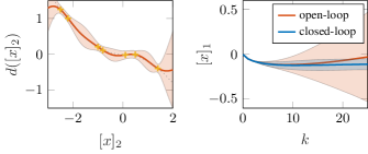
Figure 1: Propagation of uncertainty for double integrator with GP trained on a nonlinear friction term. The left plot displays the GP with $2$-$\sigma$ confidence bound, while the right plot shows the mean and $2$-$\sigma$ variance of repeated simulation runs of the system under an open-loop control sequence and closed-loop state feedback control.

In Fig. 1, the effect of state feedback on the propagation of uncertainty is exemplified. It shows the evolution over time of a double integrator with a quadratic friction term inferred by a GP. The right plot displays mean and 2-$\sigma$ variance of a number of trajectories from repeated simulations of the system with different noise realizations. Mean and variance under an open-loop control sequence derived from a linear quadratic infinite time optimal control problem are shown in red. The results with a corresponding LQR feedback law applied in closed-loop are shown in blue. As evident, open-loop input sequences can lead to rapid growth of uncertainty in the prediction, and thereby cause conservative control actions in the presence of chance constraints. Linear ancillary state feedback controllers are therefore commonly employed in stochastic and robust MPC [Bemporad1999a].

The adequate choice of ancillary feedback gains $K_{i}$ is generally a hard problem, especially if the system dynamics are highly nonlinear. A useful heuristic is to consider a linearization of the system dynamics around an approximate prediction trajectory, which in MPC applications is typically available using the solution trajectory of the previous time step. Feedback gains for the linearized system can be derived e.g. by solving a finite horizon LQR problem [Rawlings2009]. For mild or stabilizing nonlinearities, a fixed controller gain $K_{i}=K$ can be chosen to reduce computational burden, as e.g. done for the example in Fig. 1.

III-B Uncertainty Propagation

III-B1 Approximation as Normal Distributions

Because of stochastic process noise and the representation by a GP model, future predicted states result in stochastic distributions. Evaluating the posterior of a GP from an input distribution is generally intractable and the resulting distribution is not Gaussian [Quinonero-Candela2003]. While under certain assumptions on $g$, some strict over-approximations of the resulting distributions exist [Koller2018], they are typically very conservative and computationally demanding. We focus instead on computationally cheap and practical approximations at the cost of strict guarantees.

State, control input and nonlinear disturbance are approximated as jointly Gaussian distributed at every time step.

$$\begin{bmatrix}x^{\mkern-1.5mu\mathsf{T}}_{i}&u^{\mkern-1.5mu\mathsf{T}}_{i}&{(d_{i}+w_{i})}^{\mkern-1.5mu\mathsf{T}}\end{bmatrix}^{\mkern-1.5mu\mathsf{T}}\sim\mathcal{N}\left(\mu_{i},\Sigma_{i}\right)$$

$$=\mathcal{N}\!\left(\begin{bmatrix}\mu^{x}_{i}\\ \mu^{u}_{i}\\ \mu^{d}_{i}\end{bmatrix},\begin{bmatrix}\Sigma^{x}_{i}&\Sigma^{xu}_{i}&\Sigma^{xd}_{i}\\ \star&\Sigma^{u}_{i}&\Sigma^{ud}_{i}\\ \star&\star&\Sigma^{d}_{i}+\Sigma^{w}\end{bmatrix}\right)\,,$$ (9)

where $\Sigma^{u}_{i}=K_{i}\Sigma^{x}_{i}K_{i}^{\mkern-1.5mu\mathsf{T}}$, $\Sigma^{xu}_{i}=\Sigma^{x}_{i}K_{i}^{\mkern-1.5mu\mathsf{T}}$ and $\star$ denotes terms given by symmetry. Considering the covariances between states, inputs and GP, i.e. $\Sigma^{xd}$ and $\Sigma^{ud}$, is of great importance for an accurate propagation of uncertainty when the GP model $d$ is paired with a nominal system model $f$. Using a linearization of the nominal system dynamics around the mean

$$f(x,u)\approx f(\mu^{x},\mu^{u})+\nabla\!f(\mu^{x},\mu^{u})\left(\begin{bmatrix}x\\ u\end{bmatrix}-\begin{bmatrix}\mu^{x}\\ \mu^{u}\end{bmatrix}\right)\,,$$

similar to extended Kalman filtering, this permits simple update equations for the state mean and variance based on affine transformations of the Gaussian distribution in (9)

$$\mu^{x}_{i+1} =f(\mu^{x}_{i},\mu^{u}_{i})+B_{d}\mu^{d}_{i}\,,$$

$$\Sigma^{x}_{i+1} =\left[\nabla\!f(\mu_{i}^{x},\mu_{i}^{u})\ B_{d}\right]\Sigma_{i}{\left[\nabla\!f(\mu_{i}^{x},\mu_{i}^{u})\ B_{d}\right]}^{\mkern-1.5mu\mathsf{T}}\,.$$

III-B2 Gaussian Process Prediction from Uncertain Inputs

In order to define $\mu^{d}_{i},\Sigma^{d}_{i}$, $\Sigma^{xd}_{i}$ and $\Sigma^{ud}_{i}$ different approximations of the posterior of a GP from a Gaussian input have been proposed in the literature. In the following, we will give a brief overview of the most commonly used techniques, for details please refer to [Quinonero-Candela2003, Kuss2006, Deisenroth2010]. For comparison, we furthermore state the computational complexity of these methods. For notational convenience, we will use

$$\mu^{z}_{i}=\begin{bmatrix}\mu^{x}_{i}\\ \mu^{u}_{i}\end{bmatrix},\ \Sigma^{z}_{i}=\begin{bmatrix}\Sigma^{x}_{i}&\Sigma^{xu}_{i}\\ \star&\Sigma^{u}_{i}\end{bmatrix},\ \Sigma^{zd}_{i}=\begin{bmatrix}\Sigma^{xd}_{i}\\ \Sigma^{ud}_{i}\end{bmatrix}\,.$$

Mean Equivalent Approximation

A straightforward and computationally cheap approach is to evaluate (6) at the mean, such that

$$\mu^{d}_{i} =\mu^{d}(\mu^{z}_{i})\,,$$ (11a)

$$\begin{bmatrix}\Sigma^{zd}_{i}\\ \Sigma^{d}_{i}\end{bmatrix} =\begin{bmatrix}0\\ \Sigma^{d}(\mu^{z}_{i})\end{bmatrix}\,.$$ (11b)

In [Girard2002] it was demonstrated that this can lead to poor approximations for increasing prediction horizons as it neglects the accumulation of uncertainty in the GP. The fact that this approach neglects covariance between $d$ and $(x,u)$ can in addition severely deteriorate the prediction quality when paired with a nominal system $f(x,u)$. The computationally most expensive operation is the matrix multiplication in (5) for each output dimension of the GP, such that the complexity of one prediction step is $\mathcal{O}(n_{d}n_{z}M^{2})$.

Taylor Approximation

Using a first-order Taylor approximation of (5), the expected value, variance and covariance of the resulting distribution results in

$$\mu^{d}_{i} =\mu^{d}(\mu^{z}_{i})\,,$$ (12a)

$$\begin{bmatrix}\Sigma^{zd}_{i}\\ \Sigma^{d}_{i}\end{bmatrix} =\begin{bmatrix}\Sigma^{z}_{i}{(\nabla\!\mu^{d}(\mu^{z}_{i}))}^{\mkern-1.5mu\mathsf{T}}\\ \Sigma^{d}(\mu^{z}_{i})+\nabla\!\mu^{d}(\mu^{z}_{i})\Sigma^{z}_{i}{(\nabla\!\mu^{d}(\mu^{z}_{i}))}^{\mkern-1.5mu\mathsf{T}}\end{bmatrix}\,.$$ (12b)

Compared to (11) this leads to correction terms for the posterior variance and covariance, taking into account the gradient of the posterior mean and the variance of the input of the GP. The complexity of one prediction step amounts to $\mathcal{O}(n_{d}n^{2}_{z}M^{2})$. Higher order approximations are similarly possible at the expense of increased computational effort.

Exact Moment Matching

It has been shown that for certain mean and kernel functions, the first and second moments of the posterior distribution can be analytically computed [Quinonero-Candela2003]. Under the assumption that $z_{i}={[x_{i}^{\mkern-1.5mu\mathsf{T}},u_{i}^{\mkern-1.5mu\mathsf{T}}]}^{\mkern-1.5mu\mathsf{T}}$ is normally distributed, we can define

$$\mu^{d}_{i} =\mathbb{E}\left(d(z_{i})\right)\,,$$ (13a)

$$\begin{bmatrix}\Sigma^{zd}_{i}\\ \Sigma^{d}_{i}\end{bmatrix} =\begin{bmatrix}\text{cov}\left(z_{i},d(z_{i})\right)\\ \text{var}\left(d(z_{i})\right)\,.\end{bmatrix}$$ (13b)

In particular, this is possible for a zero prior mean function and the squared exponential kernel. As the procedure exactly matches first and second moments of the posterior distribution, it can be interpreted as an optimal fit of a Gaussian to the true distribution. Note that the model formulation directly allows for the inclusion of linear prior mean functions, as they can be expressed as a nominal linear system in (8), while preserving exact computations of mean and variance. The computational complexity of this approach is $\mathcal{O}(n_{d}^{2}n_{z}M^{2})$ [Deisenroth2010].

Figure 2: Comparison of prediction methods for Gaussian input ${[x]}_{2}$. The posterior distribution ${[x]}_{2}+d({[x]}_{2})$ is evaluated with the different approximation methods of Section III-B2. For reference, the true distribution is approximated by Monte Carlo simulation.

In Fig. 2 the different approximation methods are compared for a one-step prediction of the GP shown in Fig. 1 with normally distributed input. As evident, the predictions with Taylor Approximation and Moment Matching are qualitatively similar, which will typically be the case if the second derivative of the posterior mean and variance of the GP is small over the input distribution. It is furthermore apparent that the posterior distribution is not Gaussian and that the approximation as a Gaussian distribution leads to prediction error, even if the first two moments are matched exactly. This can lead to the effect that locally the Taylor Approximation provides a closer fit to the underlying distribution. The Mean Equivalent Approximation is very conservative by neglecting the covariance between ${[x]}_{2}$ and $d({[x]}_{2})$. Note that depending on the sign of the covariance it can also be overly confident.

All presented approximations scale directly with the input and output dimensions, as well as the number of data points and thus become expensive to evaluate in high dimensional spaces. This presents a challenge for predictive control approaches with GP models, which in the past have mainly focused on relatively small and slow systems [Kocijan2004, Yang2015]. Using a nominal model, however, it is possible to consider GPs that depend on only a subset of states and inputs, such that the computational burden can be significantly reduced. This is due to a reduction in the effective input dimension $n_{z}$, and more importantly due to a reduction the in necessary training points $M$ for learning in a lower dimensional space.

Remark 1.

With only slight notational changes, the presented approximation methods similarly apply to prior mean and kernel functions that are functions of only a subset of states and inputs.

Another significant reduction in the computational complexity can be achieved by employing sparse GP approaches, for which in the following we present a modification tailored to predictive control.

III-C Dynamic Sparse GPs for MPC

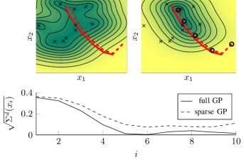
Figure 3: Illustration of dynamic sparse approximation [Hewing2018a]. Countor plot of the posterior variance of the full GP (top left) and dynamic sparse approximation (top right) with corresponding data points as black crosses. Trajectories planned by an MPC are shown as solid red lines, while the dashed lines show the prediction of the previous time step and used in the approximation, with the chosen inducing points indicated by black circles. The bottom plot shows the respective variances along the planned trajectory.

To reduce the computational burden one can make use of sparse GP approximations as outlined in Section II-D, which often comes with little deterioration of the prediction quality. A property of the task of predictive control is that it lends itself to transductive approximation schemes, meaning that we adjust the approximation based on the test points, i.e. the (future) evaluation locations in order to achieve a high fidelity local approximation. In MPC, some knowledge of the test points is typically available in terms of an approximate trajectory through the state-action space. This trajectory can, e.g., be given by the reference signal or a previous solution trajectory which will typically lie close to the current one. We therefore propose to select inducing inputs locally at each sampling time according to the prediction quality on these approximate trajectories. Ideally, the local inducing inputs would be optimized to maximize predictive quality, which is, however, not computationally feasible in the targeted millisecond sampling times. Instead, inducing inputs are selected heuristically along the approximate state input trajectory, specifically we focus here on the MPC solution computed at a previous time step.

To illustrate the procedure, we consider a simple double integrator system controlled by an MPC. Fig. 3 shows the variance $\Sigma^{d}(x)$ of a GP trained on the systems’ states. Additionally, two successive trajectories from an MPC algorithm are displayed, in which the solid red line is the current prediction, while the dashed line is the prediction trajectory from the previous iteration. The plot on the left displays the original GP, with data points marked as crosses, whereas on the right we have the sparse approximation resulting from placing inducing points along the previous solution trajectory, indicated by circles. The figure illustrates how full GP and sparse approximation match closely along the predicted trajectory of the system, while approximation quality far away from the trajectory deteriorates. Since current and previous trajectory are similar, however, local information is sufficient for computation of the MPC controller.

III-D Chance Constraint Formulation

The tractable Gaussian approximation of the state and input distribution over the prediction horizon in (9) can be used to approximate the chance constraints in (III) and (III).

We reformulate the chance constraints on state and input w.r.t. their means $\mu^{x}$, $\mu^{u}$ using constraint tightening based on the respective errors $e^{x}_{i}=\mu^{x}_{i}-x_{i}$ and $\nobreak{e^{u}_{i}=K_{i}(\mu^{x}_{i}-x_{i})}$. For this we make use of probabilistic reachable sets [Hewing2018b], an extension of the concept of reachable sets to stochastic systems, which is related to probabilistic set invariance [Kofman2012, Hewing2018].

Definition 1 (Probabilistic $i$-step Reachable Set).

A set $\mathcal{R}$ is said to be a probabilistic $i$-step reachable set ($i$-step PRS) of probability level $p$ if

$$\Pr(e_{i}\in\mathcal{R}\,|\,e_{0}=0)\geq p\,.$$

Given $i$-step PRS $\mathcal{R}^{x}$ of probability level $p_{x}$ for the state error $e^{x}_{i}$ and similarly $\mathcal{R}^{u}$ for the input $e^{u}_{i}$, we can define tightened constraints on $\mu^{x}_{i}$ and $\mu^{u}_{i}$ as

$$\mu^{x}_{i}\in\mathcal{Z} =\mathcal{X}\ominus\mathcal{R}^{x}\,,$$ (14a)

$$\mu^{u}_{i}\in\mathcal{V} =\mathcal{U}\ominus\mathcal{R}^{u}\,,$$ (14b)

where $\ominus$ denotes the Pontryagin set difference. Satisfaction of the tightened constraints (14) for the mean thereby implies satisfaction of the original constraints (III) and (III), i.e. when $\mu^{x}_{i}\in\mathcal{Z}$ we have $\Pr(x_{i}=\mu^{x}_{i}+e^{x}_{i}\in\mathcal{X})\geq\Pr(e^{x}_{i}\in\mathcal{R}^{x})\geq p_{x}$.

Under the approximation of a normal distribution of $x_{i}$, the uncertainty in each time step is fully specified by the variance matrix $\Sigma^{x}_{i}$ and $\Sigma^{u}_{i}$. The sets can then be computed as functions of these variances, i.e. $\mathcal{R}^{x}(\Sigma^{x}_{i})$ and $\mathcal{R}^{u}(\Sigma^{x}_{i})$, for instance as ellipsoidal confidence regions. The online computation and respective tightening in (14), however, is often computationally prohibitive for general convex constraint sets.

In the following, we present important cases for which a computationally cheap tightening is possible, such that it can be performed online. For brevity, we concentrate on state constraints, as input constraints can be treated analogously.

III-D1 Half-space constraints

Consider the constraint set $\mathcal{X}$ given by a single half-space constraint $\nobreak{\mathcal{X}^{hs}:=\left\{x\,\middle|h^{\mkern-1.5mu\mathsf{T}}x\leq b\right\}}$, $h\in\mathbb{R}^{n}$, $b\in\mathbb{R}_{+}$. Considering the marginal distribution of the error in the direction of the half-space $h^{\mkern-1.5mu\mathsf{T}}e^{x}_{i}\sim\mathcal{N}(0,h^{\mkern-1.5mu\mathsf{T}}\Sigma_{i}^{x}h)$ enables us to use the quantile function of a standard Gaussian random variable $\phi^{-1}(p_{x})$ at the needed probability of constraint satisfaction $p_{x}$ to see that

$$\mathcal{R}^{x}(\Sigma^{x}_{i}):=\left\{e\,\middle|h^{\mkern-1.5mu\mathsf{T}}e\leq\phi^{-1}(p_{x})\sqrt{h^{\mkern-1.5mu\mathsf{T}}\Sigma^{x}_{i}h}\right\}$$

is an $i$-step PRS of probability level $p_{x}$. In this case, evaluating the Pontryagin difference in (14) is straightforward and we can directly define the tightened constraint on the state mean

$$\mathcal{Z}^{hs}(\Sigma^{x}_{i}):=\left\{z\,\middle|h^{\mkern-1.5mu\mathsf{T}}z\leq b-\phi^{-1}(p_{x})\sqrt{h^{\mkern-1.5mu\mathsf{T}}\Sigma^{x}_{i}h}\right\}\,.$$

Remark 2.

A tightening for slab constraints $\nobreak{\mathcal{X}^{sl}=\left\{x\,\middle||h^{\mkern-1.5mu\mathsf{T}}x|\leq b\right\}}$ can be similarly derived as

$$\mathcal{Z}^{sl}(\Sigma^{x}_{i}):=\left\{z\,\middle||h^{\mkern-1.5mu\mathsf{T}}z|\leq b-\phi^{-1}\!\left(\frac{p_{x}\!+\!1}{2}\right)\sqrt{h^{\mkern-1.5mu\mathsf{T}}\Sigma^{x}_{i}h}\right\}\,.$$

III-D2 Polytopic Constraints

Consider polytopic constraints, given as the intersection of $n_{j}$ half-spaces

$$\mathcal{X}^{p}=\left\{x\,\middle|h^{\mkern-1.5mu\mathsf{T}}_{j}x\leq b_{j}\ \forall j=1,\ldots,n_{j}\right\}\,.$$

Making use of ellipsoidal PRS for Gaussian random variables one can formulate a semidefinite program to tighten constraints [Zhou2013, Schildbach2015], which is computationally demanding to solve online. Computationally cheaper approaches typically rely on more conservative bounds. One such bound is given by Boole’s inequality

$$\Pr(E_{1}\wedge E_{2})\leq\Pr(E_{1})+\Pr(E_{2})\,,$$ (15)

which allows for the definition of polytopic PRS based on individual half-spaces. We present two possibilities, the first of which is based on bounding the violation probability of the individual polytope faces, and a second which considers the marginal distributions of $e^{x}_{i}$.

PRS based on polytope faces

Similar to the treatment of half space constraints, we can define a PRS on the state error $e^{x}$ which is aligned with the considered constraints. Using Boole’s inequality (15), we have that

$$\mathcal{R}^{x}(\Sigma^{x}_{i})=$$

$$\left\{e\,\middle|h_{j}^{\mkern-1.5mu\mathsf{T}}e\leq\phi^{-1}\!\left(1\!-\!\frac{1\!-\!p_{x}}{n_{j}}\right)\sqrt{h_{j}^{\mkern-1.5mu\mathsf{T}}\Sigma^{x}_{i}h_{j}}\ \forall j=1,\ldots,n_{j}\right\}$$

is a PRS of probability level $p_{x}$. The tightening results in

$$\mathcal{Z}^{p}(\Sigma^{x}_{i})=$$

$$\left\{z\,\middle|h_{j}^{\mkern-1.5mu\mathsf{T}}z\leq b_{j}-\phi^{-1}\!\left(\!1\!-\!\frac{1\!-\!p_{x}}{n_{j}}\!\right)\!\sqrt{h_{j}^{\mkern-1.5mu\mathsf{T}}\Sigma^{x}_{i}h_{j}}\ \forall j=1,\ldots,n_{j}\right\}$$

which scales with the number of faces of the polytope and can therefore be quite conservative if the polytope has many (similar) faces.

PRS based on marginal distributions

Alternatively, one can define a PRS based on the marginal distribution of the error $e^{x}$ in each dimension, which therefore scales with the state dimension. We use Boole’s inequality (15) with Remark 2 directly on marginal distributions in each dimension of the state to define a box-shaped PRS of probability level $p_{x}$

$$\mathcal{R}^{x}(\Sigma^{x}_{i})=\left\{e\,\middle||[e]_{j}|\leq\phi^{-1}(\bar{p})\sqrt{[\Sigma^{x}_{i}]_{j,j}}\ \forall j=1,\ldots,n_{x}\right\}\,.$$

with $\bar{p}=1-\left(\!\frac{1}{n_{x}}\!-\!\frac{p_{x}\!+\!1}{2n_{x}}\right)$. To compute the Pontryagin difference (14) we make use of the following Lemma.

Lemma 1.

Let $\mathcal{A}=\left\{x\,\middle|Hx\leq b\right\}$ be a polytope and $\nobreak{\mathcal{B}=\left\{e\,\middle|-r\leq e\leq r,\,r\in\mathbb{R}^{n}_{+}\right\}}$, a box in $\mathbb{R}^{n}$.

Then $\mathcal{A}\ominus\mathcal{B}=\left\{x\,\middle|Hx\leq b-|H|r\right\}$, where $|H|$ is the element-wise absolute value.

Proof.

From definition of the Pontryagin difference we have

$$\mathcal{A}\ominus\mathcal{B} =\left\{x\,\middle|x+e\in\mathcal{A}\ \forall e\in\mathcal{B}\right\}$$

$$=\left\{x\,\middle|H(x+e)\leq b\ \forall e\in\mathcal{B}\right\}$$

$$=\left\{x\,\middle|[H]_{j,\cdot}x\leq[b]_{j}-\max_{e\in\mathcal{B}}[H]_{j,\cdot}e\ \forall j=1,\ldots,n\right\}$$

$$=\left\{x\,\middle|[H]_{j,\cdot}x\leq[b]_{j}-|[H]_{j,\cdot}|r\,\forall j=1,\ldots,n\right\}$$

$$=\left\{x\,\middle|Hx\leq b-|H|r\right\}\,,$$

proving the result. ∎

The resulting tightened set is therefore

$$\mathcal{Z}^{p}(\Sigma^{x}_{i})=\left\{z\,\middle|Hz\leq\tilde{b}(\Sigma^{x}_{i})\right\}$$

with $\tilde{b}(\Sigma^{x}_{i})=b-|H|\phi^{-1}(\bar{p})\sqrt{\operatorname{\text{diag}}(\Sigma^{x}_{i})}$, where $\operatorname{\text{diag}}(\cdot)$ is the vector of diagonal elements and the square root of the vector is taken element wise.

Remark 3.

Treating polytopic constraints through (15) can lead to undesired and conservative individual constraints [Lorenzen2017]. Practically, it can therefore be beneficial to constrain the probability of violating each individual half-space constraint.

III-E Cost Function

Given the approximate joint normal distribution of state and input, the cost function (III) can be evaluated using standard stochastic formulations. For simplicity, we focus here on costs in form of expected values, which encompass most stochastic objectives typically considered. While the expected value for general cost functions needs to be computed numerically, there exist a number of functions for which evaluation based on mean and variance information can be analytically expressed and is computationally cheap. The most prominent example for tracking tasks is a quadratic cost on states and inputs

$$l(x_{i}-x_{i}^{r},u_{i}-u_{i}^{r})=\|x_{i}-x_{i}^{r}\|_{Q}^{2}+\|u_{i}-u_{i}^{r}\|_{R}^{2}$$ (16)

with appropriate weight matrices $Q$ and $R$, typically satisfying $Q\succeq 0$ and $R\succ 0$, resulting in

$$\operatorname{\mathbb{E}}\left(l(x_{i}-x_{i}^{r},u_{i}-u_{i}^{r})\right)=$$

$$\|\mu^{x}_{i}-x_{i}^{r}\|_{Q}^{2}+\operatorname{\text{tr}}(Q\Sigma^{x}_{i})+\|\mu^{u}_{i}-u_{i}^{r}\|_{R}^{2}+\operatorname{\text{tr}}(R\Sigma^{u}_{i})\,.$$

Further examples include a saturating cost [Deisenroth2010], risk sensitive costs [Whittle1981] or radial basis function networks [Kamthe2018].

We refer to the evaluation of the expected value (III) in terms of mean and variance as

$$\operatorname{\mathbb{E}}\left(l(x_{i}-x_{i}^{r},u_{i}-u_{i}^{r})\right)=c(\mu^{x}_{i}-x_{i}^{r},\mu^{u}_{i}-u_{i}^{r},\Sigma^{x}_{i})$$

and similarly $c_{f}(\mu^{x}_{N}-x_{N}^{r},\Sigma^{x}_{N})$ for the terminal cost.

Remark 4.

While many performance indices can be expressed as expected values, there exist various stochastic cost measures, such as conditional value-at-risk. Given the approximate state distributions, many can be similarly considered.

III-F Tractable MPC Formulation with GP Model

By bringing together the approximations of the previous sections, the following tractable approximation of the MPC problem (III) can be derived: {μ^u_i} c_f(μ^x_N​-​x^r_N, Σ^x_N) + ∑_i=0^N-1 c(μ^x_i​-​x^r_i, μ^u_i​-​u^r_i, Σ^x_i) μ^x_i+1= f(μ^x_i,μ^u_i) + B_d μ^d_i Σ^x_i+1= [∇​ f(μ_i^x,μ^u_i)  B_d ] Σ_i[∇​ f(μ_i^x,μ^u_i)  B_d ]^T μ^x_i+1 ∈Z(Σ^x_i+1) μ^u_i ∈V(Σ^x_i) μ^d_i, Σ_i according to (9) and (11), (12) or (13) μ^x_0= x(k), Σ^x_0 = 0 for $i=0,\ldots,N\!-\!1$. The resulting optimal control law is obtained in a receding horizon fashion as $\kappa(x(k))=\mu^{u*}_{0}$, where $\mu^{u*}_{0}$ is the first element of the optimal control sequence $\{\mu^{u*}_{0},\ldots,\mu^{u*}_{N}\}$ obtained from solving (III-F) at state $x(k)$.

The presented formulation of the MPC problem with a GP-based model results in a non-convex optimization problem. Assuming twice differentiability of kernel and prior mean function, second-order derivative information of all quantities is available. Problems of this form can typically be solved to local optima using Sequential Quadratic Programming (SQP) or nonlinear interior-point methods [Diehl2009]. There exist a number of general-purpose solvers that can be applied to solve this class of optimization problems, e.g. the openly available IPOPT [Wachter2006]. In addition, there are specialized solvers that exploit the structure of predictive control problems, such as ACADO [Houska2011] or FORCES Pro [FORCESPro, Zanelli2017], which implements a nonlinear interior point method. Derivative information can be automatically generated using automated differentiation tools, such as CASADI [Andersson2013].

In the following, we demonstrate the proposed algorithm and its properties using one simulation and one experimental example. The first is an illustrative example of an autonomous underwater vehicle (AUV) which, around a trim point, is well described by nominal linear dynamics but is subject to nonlinear friction effects for larger deviations. The second example is a hardware implementation demonstrating the approach for autonomous racing of miniature race cars which are described by a nonlinear nominal model. While model complexity and small sampling times require additional approximations in this second example, we show that we can leverage key benefits of the proposed approach in a highly demanding real-world application.

IV Online Learning for Autonomous Underwater Vehicle

We consider the depth control of an autonomous underwater vehicle (AUV). The vehicle is described by a nonlinear continuous-time model of the vehicle at constant surge velocity as ground truth and for simulation purposes [Naik2007]. Around a trim point of purely horizontal movement, the states and input of the system are

${[x]}_{1}$

the pitch angle relative to trim point [$\mathrm{r}\mathrm{a}\mathrm{d}$],

${[x]}_{2}$

the heave velocity relative to trim point [$\mathrm{m}\mathrm{/}\mathrm{s}$],

${[x]}_{3}$

the pitch velocity [$\mathrm{r}\mathrm{a}\mathrm{d}\mathrm{/}\mathrm{s}$],

$u$

the stern rudder deflection around trim point [$\mathrm{r}\mathrm{a}\mathrm{d}$].

We assume that an approximate linear system model is given, which in practice can be established using methods of linear system identification around the trim point of the system. Using a zero-order hold discretization of the linear part of the model with $T_{s}=$100\text{\,}\mathrm{m}\mathrm{s}$$ we obtain

$$x(k\!+\!1) =Ax(k)+Bu(k)+B_{d}\left(g(x(k))+w(k)\right)\,,$$

which is in the form of (1). The nonlinearity results from friction effects when moving in the water, which is therefore modeled as only affecting the (continuous time) velocity states,

$$B_{d}=\begin{bmatrix}0&\frac{T_{s}^{2}}{2}\\ T_{s}&0\\ 0&T_{s}\end{bmatrix},\ g(x(k))=g({[x(k)]}_{2},{[x(k)]}_{3}):\mathbb{R}^{2}\rightarrow\mathbb{R}^{2}\,.$$

Note that the eigenvalues of $A$ are given by $\lambda=\{1.1,1.03,1,0.727\}$, i.e. the linear system has one integrating and two unstable modes.

In the considered scenario, the goal is to track reference changes from the original zero set point to a pitch angle of $30\degree$, back to zero and then to $45\degree$. We furthermore consider a safety state constraint on the pitch angle of at least $10\degree$ below the reference, as well as input constraints corresponding to $\pm 20\degree$ rudder deflection. In this example, we treat the case of online learning, that is we start without any data about the nonlinearity $g$, collect measurement data during operation and enhance performance online.

IV-A GP-based Reference Tracking Controller

GP data $\mathcal{D}=\{\mathbf{y},\mathbf{z}\}$ is generated by calculating the deviation of the linear model from the measured states, as described in Section II-C, where the input data is reduced to the velocity states $z_{j}=[{[x_{j}]}_{2},{[x_{j}]}_{3}]^{\mkern-1.5mu\mathsf{T}}$. Data is continuously updated during the closed-loop run. Specifically, we consider a new data point every 5 time steps, and keep track of 30 data points by discarding the oldest when adding a new point. The training data is initialized with 30 data points of zero input and zero output. We employ a squared exponential kernel (3) for both output dimensions with fixed hyperparameters $L_{1}=L_{2}=\text{diag}([0.35,0.15]^{\mkern-1.5mu\mathsf{T}})$, and variances $\sigma_{f,1}^{2}=0.04$ and $\sigma_{f,2}^{2}=0.25$.

We use a quadratic stage cost as in (16), with weight matrices $Q=\text{diag}([1,0,10,0.5^{\mkern-1.5mu\mathsf{T}}])$, $R=20$ and a prediction horizon $N=35$ to track a pitch angle reference. The terminal cost $P$ is chosen according to the solution of the associated discrete-time algebraic Riccati equation, i.e. the LQR cost. As ancillary linear controller $K_{i}$, an infinite horizon LQR control law based on the linear nominal model is designed using the same weights as in the MPC and used in all prediction steps $i$. This stabilizes the linear system and reduces uncertainty growth over the prediction horizon. To propagate the uncertainties associated with the GP we make use of the Taylor Approximation outlined in Section III-B2. Constraints are introduced based on Remark 3 considering a maximum probability of individual constraint violation of $2.28\%$, corresponding to a $2$-$\sigma$ confidence bound. The MPC optimization problem (III-F) is solved using FORCES Pro [FORCESPro, Zanelli2017].

IV-B Results

Figure 4: Predicted pitch angle ${[x]}_{1}$ and rudder deflection $u$. Dotted lines are the mean prediction and shaded the $2$-$\sigma$ confidence region. The dashed lines show the corresponding state and input constraints, while the black line is the pitch angle reference.

Fig. 4 shows the prediction of the GP-based MPC for the first reference change from $0\degree$ to $30\degree$. Since no data was collected on the state trajectory necessary for this change, the predicted state and input trajectories are uncertain and a safety margin to the state constraint at the end of the horizon is enforced. The resulting closed-loop trajectory, during which the system learns from online data, is displayed in the top plot of Fig. LABEL:fg:auv_comp. For comparison, we run the same simulation with a soft constrained linear MPC formulation with the same cost function, which does not consider nonlinearities or uncertainties in the dynamics, shown in the bottom plot. The results demonstrate improved performance of the GP-based MPC over the linear MPC, especially with regard to constraint satisfaction. The constraint on minimum pitch angle is violated under the linear MPC control law during both reference changes, even though the soft constraint is chosen as an exact penalty function such that constraints are always satisfied, if possible. Fig. LABEL:fg:auv_err exemplifies the residual model error during the closed-loop simulation applying the GP-based controller, as well as the predicted $2$-$\sigma$ residual error bound of the GP. We observe the largest error during reference changes, which are anticipated by the GP-uncertainty, overall matching the resulting residual errors well.