Extragalactic Background Light: a measurement at 400 nm using dark cloud shadow
I. Low surface brightness spectrophotometry in the area of Lynds 1642

Abstract

We present the method and observations for the measurement of the Extragalactic Background Light (EBL) utilizing the shadowing effect of a dark cloud. We measure the surface brightness difference between the opaque cloud core and its unobscured surroundings. In the difference the large atmospheric and Zodiacal light components are eliminated and the only remaining foreground component is the scattered starlight from the cloud itself. Although much smaller, its separation is the key problem in the method. For its separation we use spectroscopy. While the scattered starlight has the characteristic Fraunhofer lines and 400 nm discontinuity the EBL spectrum is smooth and without these features. Medium resolution spectrophotometry at $\lambda$ = 380 - 580 nm was performed with VLT/FORS at ESO of the surface brightness in and around the high-galactic-latitude dark cloud Lynds 1642. Besides the spectrum for the core with $A_{V}\ga 15$ mag, further spectra were obtained for intermediate-opacity cloud positions. They are used as proxy for the spectrum of the impinging starlight spectrum and facilitate the separation of the scattered starlight (cf. Paper II, Mattila et al. 2017b). Our spectra reach a precision of $\la 0.5$ $10^{-9}$ erg cm^-2s^-1sr^-1Å^-1  as required to measure an EBL intensity in range of $\sim$1 to a few times $10^{-9}$ erg cm^-2s^-1sr^-1Å^-1 . Because all surface brightness components are measured using the same equipment the method does not require unusually high absolute calibration accuracy, a condition which has been a problem for some previous EBL projects.

1 Introduction

The importance of the Extragalactic Background Light (EBL) for cosmology has long been recognized, see e.g. Partridge & Peebles (1967) and for a review Longair (1995). The EBL at UV, optical and near infrared wavelengths consists of the integrated light of all unresolved galaxies along the line of sight plus any contributions by intergalactic gas and dust and by hypothetical decaying relic particles. A large fraction of the energy released in the Universe since the recombination epoch is expected to be contained in the EBL. An important aspect is the balance between the UV-to-NIR ($\lambda\approx 0.1-3~{}\mu$m) and the mid-to-far infrared ($\lambda\approx 5-300~{}\mu$m) EBL: what is lost through absorption by dust in the UV–NIR will re-appear as emission in the mid-to-far IR. This aspect is strongly emphasized by the detection of the far infrared EBL (Hauser et al., 1998; Puget et al., 1996; Juvela et al., 2009). Some central, but still largely open astrophysical problems to which EBL measurements can shed new light include the formation and early evolution of galaxies and the star formation history of the Universe. There may also be significant numbers of Low Surface Brightness galaxies, intergalactic star clusters and stars escaping detection as discrete objects but contributing to the cumulative EBL (Väisänen, 1996; Zemcov et al., 2014). In observational cosmology the nature of a background brightness measurement has, in principle, an advantage over the number count observations. When counting galaxies, whether in magnitude or redshift bins, one needs to consider many kinds of selection effects which affect the completeness of the sample. The measurement of the EBL is not plagued by this particular problem. However, it is hampered by the foreground components, much larger than the EBL itself, and their elimination or accurate evaluation is of key importance for the direct photometric measurement of the EBL (for a review see Mattila & Schnur 1990).

1.1 Recent EBL measurements

Bernstein et al. (2002a) announced ’the first detection’ of the EBL at 300, 550, and 800 nm. In their method they used a combination of space borne (HST) and ground based measurements. While the total sky brightness photometry with HST was free of atmospheric effects the contribution by the Zodiacal Light, $\ga 95\%$ of the total sky, had to be measured from the ground with another telescope. However, in the Zodiacal Light measurement they neglected some effects of the atmospheric scattered light and were not able to achieve for their surface photometry calibration the absolute systematic accuracy of $\la 0.5\%$, required for both the HST and the ground based telescope (see Mattila 2003). Therefore, the claim for a detection of the EBL appeared premature. After reanalysis of their systematic errors Bernstein et al. (2005) and Bernstein (2007) came to the conclusion that
’ … the complexity of the corrections required to do absolute surface (spectro)photometry from the ground make it impossible to achieve 1% accuracy in the calibration of the ZL’, and ’…the only promising strategy … is to perform all measurements with the same instrument, so that the majority of corrections and foreground subtractions can be done in a relative sense, before the absolute calibration is applied.’

Matsuoka et al. (2011) have re-analyzed the Pioneer 10/11 Imaging Photopolarimeter sky background data which were used already by Toller (1983) to derive an upper limit to the EBL at 440 nm. They have announced a detection of the EBL at 440 and 640 nm at 1.5 to 2$\sigma$ level. Although free of the ZL contamination, also this method is plagued by the problem that the EBL is merely a small difference between two large quantities: the total sky brightness as seen by Pioneer 10/11 and the Integrated Starlight which makes up $\ga 95\%$ of the Pioneer 10/11 total sky brightness signal. Thus, for a detection of the EBL a very accurate ($\la 1\%$) photometric calibration of the Pioneer 10/11 surface photometry against the diverse photometric systems of star catalogues used for the ISL summation is required.

Recently, the Long Range Reconnaissance Imager instrument aboard NASA’s New Horizons mission acquired optical broad band (440 – 870 nm) sky background measurements during its cruise phase beyond Jupiter’s orbit. While being free of ZL, and much less infuenced by starlight contamination than the Pioneer 10/11 photometry, the limiting factor according to the analysis of Zemcov et al. (2017) was the model-dependent estimation of the Diffuse Galactic Light. Their 2$\sigma$ upper limit was $\sim$2 times as high as the integrated light from galaxy counts.

In recent years an indirect method based on the absorption of TeV gamma-ray radiation by the intervening intergalactic radiation field has been used to probe, at first, the mid-IR EBL (Aharonian et al., 2006). More recently it has become possible to probe also the optical EBL (Ackermann et. al., 2012; H.E.S.S. Collaboration, 2013; Domínguez et al., 2013; Biteau & Williams, 2015). While this method is free of the problems caused by the night sky component separation it does include uncertainties of the intrinsic spectral energy distributions of the blazars, used as probes for the gamma-ray absorption effects.

1.2 The present EBL measurement project

In the present situation it appears desirable to obtain another direct photometric measurement of the EBL with an independent method. We are using the dark cloud shadow method as presented by Mattila (1976) and Mattila & Schnur (1990). It utilizes one and the same instrument for all sky components and is virtually free of the large foreground components, i.e. the Airglow (AGL), the Zodiacal Light (ZL), the Integrated Starlight (ISL), as well as the tropospheric scattered light which together with the AGL forms the Atmospheric Diffuse Light (ADL). The Diffuse Galactic Light (DGL), which stands for the starlight that has been scattered by the widely distributed interstellar dust, is eliminated as far as it originates in front of the dark cloud. The main task now is to account for the surface brightness (scattered light) of the dark cloud. In the following we will refer to the components of the light of the night sky by the abbreviations given here.

The rest of this paper is organized as follows. The dark cloud shadow method for the EBL separation is described in Section 2. In Section 3 the selection of observing positions in the area of the high-latitude dark nebula L 1642 is described. Long-slit intermediate resolution spectroscopic observations, $\lambda=380-580$ nm, were carried out using the FORS1 and FORS2 instruments (Appenzeller et al., 1998) at the Very Large Telescope (VLT) of ESO and are described in Section 4. The data reduction procedures are presented in Section 5. In Section 6 we present the calibration methods and in Section 7 the corrections for differential effects caused by the ZL, AGL, tropospheric scattered light, and straylight from stars outside the measuring aperture. Section 8 gives the observational results. Preliminary results of this project have been presented in Mattila et al. (2012).

The Paper has three appendices containing supporting data. Appendix A describes the details of the small corrections for differential effects caused by the ZL and AGL. In Appendix B we present measurements of the straylight aureole of a star and the straylight correction estimates. Appendix C describes supporting intermediate band optical and 200 $\mu$m far-IR surface photometry of the L 1642 cloud area.

The separation of the EBL from the scattered light of the dark nebula is described in the accompanying Paper II (Mattila et al., 2017b).

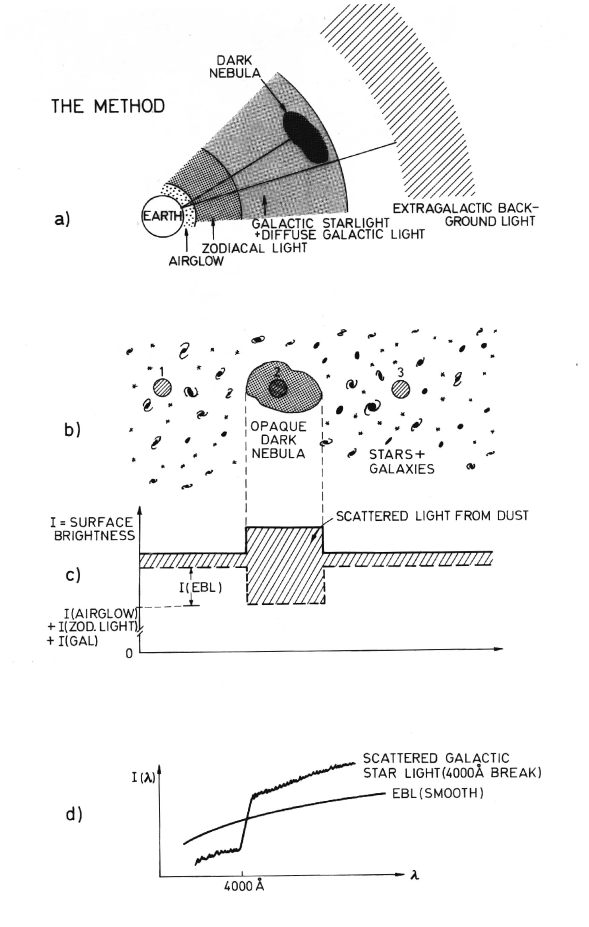
Figure 1: The principle of EBL measurement with the dark cloud shadow method. (a) an overview of the geometry of the night sky components involved; (b) sketch of the view on the sky with three observing positions indicated: ’2’ for a field in the centre of the dark cloud, ’1’ and ’3’ for fields in transparent areas outside the dark cloud; (c) If the scattered light from the interstellar dust were zero (i.e. if the grain albedo $a=0$), then the difference in surface brightness between a transparent comparison area and the dark cloud would be due to the EBL only, and an opaque nebula would be darker by the amount of the EBL intensity (dashed line). The scattered light is not zero, however. A dark cloud in the interstellar space is exposed to the radiation field of the integrated Galactic starlight giving rise to diffuse scattered light (shaded area) which is particularly strong in the direction of the dark cloud. Outside the dark cloud there is still scattered light, even at high galactic latitudes, present as a general DGL component, though at a much lower level. (d) We utilize the difference in the spectral shapes of the EBL and the integrated Galactic starlight for their separation.

Figure 2: The synthetic spectrum of integrated Galactic starlight, mean over the sky, smoothed to our FORS resolution of 1.1 nm, as seen by a cloud at a distance of 85 pc off the Galactic plane near the Sun. For the Galactic model and the stellar library, see Appendix A of Paper II. Notice the several strong Fraunhofer lines and the discontinuity at 400 nm.

2 The dark cloud shadow method

The method utilizes the shadow effect of a dark cloud on the background light. The difference of the night-sky brightness in the direction of a high galactic latitude dark cloud and a surrounding area that is (almost) free of obscuring dust is due to two components only: (1) the EBL, and (2) the starlight that has been diffusely scattered by interstellar dust in the cloud and, to a smaller extent, also by diffuse dust in its surroundings. Three large foreground components, i.e. the ZL, the AGL, and the tropospheric scattered light, are eliminated. Fig. 1 gives an overview of the dark cloud method.

Because the intensity of the scattered light is expected to be similar or larger than the EBL, its separation is the main task in our method. This can be achieved by means of spectroscopy. While the scattered Galactic starlight spectrum has the characteristic stellar Fraunhofer lines and the discontinuity at 400 nm the EBL spectrum is a smooth one without these features (see Fig. 1d and Fig. 2). This can be understood because the radiation from galaxies and other luminous matter over a vast redshift range contributes to the EBL, thus washing out any spectral lines or discontinuities.

3 The target cloud and observed positions

The high galactic latitude dark nebula Lynds 1642 ($l=210\aas@@fstack{\circ}9,b=-36\aas@@fstack{\circ}7$) has been chosen as our target. Its distance has been determined to be between 110 and 170 pc (Hearty et al., 2000) corresponding to a $z$-distance of -65 to -100 pc. It has high obscuration ($A_{\mathrm{V}}\ga 15$ mag) in the centre. On the other hand, there are areas of good transparency ($A_{\mathrm{V}}\approx 0.15$ mag) in its immediate surroundings within $\sim 2\degr$. Its declination of -14$\aas@@fstack{\circ}$5 allows observations at low airmasses from Paranal. In Fig. 3 our measuring positions for the VLT/FORS spectra (for which also intermediate band photometry was done) are shown as squares and the positions with intermediate band photometry only as circles (see Appendix C). The coordinates and line-of-sight extinction estimates for the spectroscopy positions are given in Table 1. The extinction estimate $A_{\mathrm{V}}$ for position Pos8 was derived from dedicated JHK photometry of background stars using the SOFI/NTT instrument at ESO/La Silla (K. Lehtinen, private communication). For the other positions the $A_{\mathrm{V}}$ values were derived using ISO/ISOPHOT (Kessler et al., 1996; Lemke et al., 1996) far IR (200 $\mu$m) absolute photometry, with Zodiacal emission and Cosmic Infrared Background subtracted, and scaled against 2MASS JHK near IR extinction measurements (see Appendix C for details).

Stamps of 10x10 arcmin size centred on the VLT/FORS positions, adopted from Digital Sky Survey blue plates, are shown in the margins: the high-opacity central position Pos8 with $A_{V}\ga 15$ mag is shown in upper left, followed clockwise by the two intermediate-opacity positions, Pos9 and Pos42 with $A_{V}\approx 1$ mag, and then the transparent OFF-cloud positions with $A_{V}\approx 0.15$ mag.

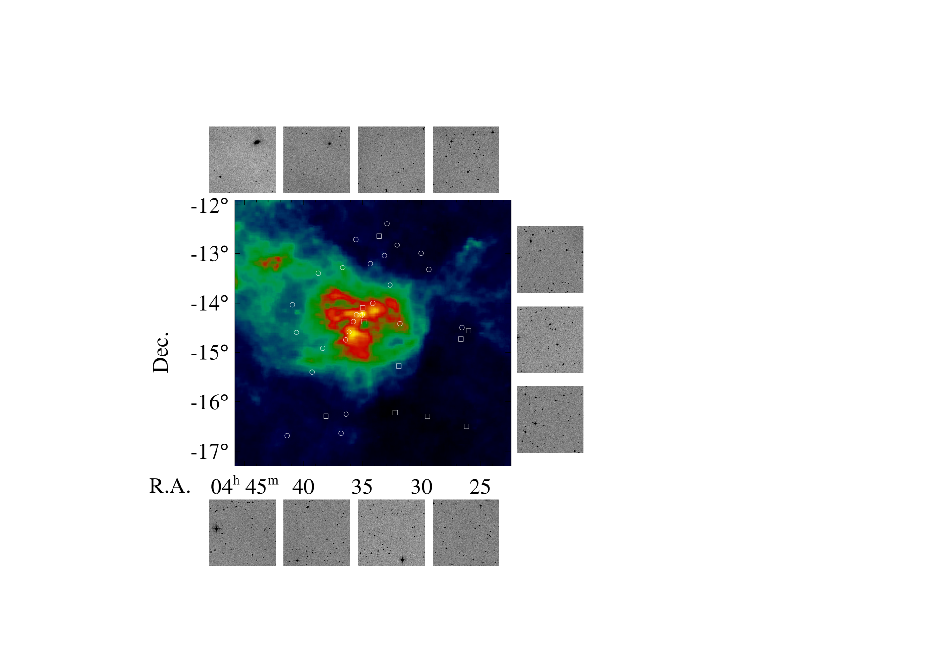
Figure 3: The observed positions in the L 1642 cloud area superimposed on a map of IRAS 100 $\mu$m emission that serves as a qualitative proxy for the interstellar extinction through the cloud. Positions observed spectroscopically (VLT/FORS) and photometrically (La Silla 1-m/50-cm) are shown as squares, and positions observed only photometrically as circles. The stamps around the map are 10 x 10 arcmin extracts from the $B$ band DSS, and are for the positions (clockwise from upper left hand corner): Pos8, 9, 42, 13, 18, 34, 36, 32, 24, 25, and 20

Table 1: Data for the positions in and around L 1642 observed in long slit mode with FORS. For the standard position POS08 the observed slit positions deviate in some cases by up to 25 arcsec from those given in the table. They are still well within the starless dark core. See also Table 2.

Name	R.A.(J2000)	Decl.(J2000)	I(200 $\mu$m)($\pm\sigma$)	$A_{\mathrm{V}}$
			[MJy sr-1]	[mag]
POS08	04:35:11.2	-14:16:26	58.78 (1.5)	$\ga 15$
POS09	04:34:59.5	-14:06:36	23.97 (0.5)	1.17
POS42	04:34:54.4	-14:23:29	18.14 (1.0)	0.86
POS18	04:33:37.0	-12:39:25	5.92 (0.21)	0.22
POS20	04:38:04.9	-16:18:14	6.49 (0.17)	0.25
POS24	04:29:31.0	-16:18:12	3.57 (0.10)	0.09
POS25	04:32:13.4	-16:13:59	3.71 (0.06)	0.10
POS32	04:26:12.3	-16:30:21	3.72 (0.10)	0.10
POS34a	04:26:44.2	-14:44:16	4.57 (0.09)	0.15
POS34b	04:26:54.6	-14:44:23	4.57 (0.09)	0.15
POS36	04:26:07.7	-14:34:32	4.40 (0.13)	0.14

4 Observations

4.1 Observing procedure

All our surface brightness measurements were made differentially, i.e. relative to a ’standard position’ (Pos8) in the centre of the cloud. The journal of observations is given in Table 2. The observing procedures for the OFF-cloud background positions, at $\sim 2\degr$ distance from Pos8, and for the two IN-cloud positions Pos9 and Pos42 within $\sim$10 arcmin of Pos8 were as follows:

4.1.1 OFF-cloud positions.

In most cases the ’programme position PosN’ measurement was bracketed by equally long ’standard position’ measurements before, $I_{1}$(Pos8), and after, $I_{2}$(Pos8), and the surface brightness difference was calculated from:

$$\Delta I_{\rm obs}{\rm(Pos8-PosN)}={}$$ (1)

$${}=\frac{1}{2}[I_{1}{\rm(Pos8)}+I_{2}{\rm(Pos8)}]-I{\rm(PosN)}$$

In two cases, because of more favourable airglow conditions, the difference was formed between one ’standard position’ measurement bracketed by two different ’programme position’ measurements before and after (Pos18/24 on 2003-10-20 and Pos32/25 on 2004-01-25) and the surface brightness difference was calculated from:

$$\Delta I_{\rm obs}{\rm(Pos8-PosN1/N2)}={}$$ (2)

$${}=I{\rm(Pos8)}-\frac{1}{2}[I{\rm(PosN1)}+I{\rm(PosN2)}]$$

In these cases we obtain the mean of the surface brightness differences $\Delta I_{\rm obs}$(Pos8 – PosN1) and $\Delta I_{\rm obs}$(Pos8 – PosN2).

For an efficient elimination of the airglow variations the measuring cycle had to be as short as possible. A cycle time of 20–25 min per phase (integration + overhead time) was short enough to give sufficiently small AGL changes in $\sim$60% of the cases. This still made the time spent for overheads (read-out time, telescope movements) a tolerable fraction (ca. 25–30%) of the total telescope time. On the other hand, for much shorter integration times the read-out noise would start to become a disturbingly large fraction as compared to the photon noise, and the fraction of overhead time would increase.

For a time difference of $\sim$50 min between the two ’standard position’ measurements, ’before’ and ’after’, the sky surface brightness over the wavelength range 375–500 nm changed by $\la 5$ $10^{-9}$ erg cm^-2s^-1sr^-1Å^-1  for the best $\sim$ 30% of the observations. These will be called the ’Master spectra’. They are listed as the first four items in Table 2. For another $\sim$ 30% of the observations the change over the wavelength range 375–580 nm was $\la$ 10 $10^{-9}$ erg cm^-2s^-1sr^-1Å^-1 ; these are called the ’Secondary spectra’ and they are listed as the next six items in Table 2. In the case of occasional still larger sky level changes of $>$ 10 $10^{-9}$ erg cm^-2s^-1sr^-1Å^-1  the data were omitted. We note that, as described in Appendix C for the photometric measurements, the use of a parallel monitor telescope can eliminate most of the airglow variations. An arrangement with a spectroscopic monitor telescope was, however, not feasible for the present observations.

We demonstrate in Fig. 4 the different steps of our observing procedure. The total sky spectrum for Pos24 is shown as red while the standard position Pos8 spectra ’before’ and ’after’ are shown as black and blue lines. The difference spectrum $\Delta I_{\rm obs}$(Pos8 – Pos24) is shown as blue and the difference between the two Pos8 measurements as the green line. The airglow variability during this night was low, $\la$ 5 $10^{-9}$ erg cm^-2s^-1sr^-1Å^-1  over the wavelength range 375–500 nm, qualifying this observation to be included in the ’Master spectra’. Notice that while the difference spectrum of the two Pos8 observations still shows substantial residuals of the strong airglow features, they have almost completely disappeared in the $\Delta I_{\rm obs}$(Pos8 – Pos24) spectrum thanks to a linear variability with time of the airglow during this observation. The spectra displayed in Fig. 4 are calibrated but are not corrected for extinction or other atmospheric effects, i.e. they show the spectra as observed at the ground level. For the transformation to above-the-atmosphere see Sections 6.3 and 7.

4.1.2 IN-cloud positions 9 and 42.

In the case of the two IN-cloud positions it was possible to combine the observations of ON and OFF position into one Observing Block with several consecutive observing pairs taken by shifting the telescope pointing along the slit. This way the overhead time per ON-OFF measurement pair was reduced to $\sim$12 min making an integration time per position of 5 min a feasible choice. In these cases the position angle of the slit had to be adjusted along the direction between ON and OFF positions.

Table 2: Journal of observations. Coordinates, observing dates, integration times, slit position angles (from N to E) and detector chips (1, 2, or both) are given. The airmass $X$, airmass difference $\Delta X$, the ZL intensity $I_{\rm ZL}$ and ZL difference $\Delta I_{\rm ZL}$ are given in columns (7) and (8). The differences are in the sense Pos8 minus PosN. The ZL values are at $\lambda=500$ nm in units of $10^{-9}$ erg cm^-2s^-1sr^-1Å^-1 .

Posit-	R.A.(J2000)	Decl.(J2000)	Date and	Slit P.A.	Obs.cycle	Airm $X$	$I_{\rm ZL}$	Weight
ion			ESO Period	Chip(s)	Int.time	$\Delta X$	$\Delta I_{\rm ZL}$
(1)	(2)	(3)	(4)	(5)	(6)	(7)	(8)	(9)
Master spectra
POS18	04:33:37.0	-12:39:25	2003-10-20	0.0	24-8-8-18	1.073	102	1
POS08	04:35:11.2	-14:16:26	72	1	1042	-0.003	-0.4
POS24	04:29:31.0	-16:18:12
POS24	04:29:31.0	-16:18:12	2003-10-20	0.0	8-24-8	1.146	103	1
POS08	04:35:11.2	-14:16:26	72	1	1042	0.032	1.4
POS24	04:29:31.4	-16:18:16	2004-09-18	-90.0	8-24-8	1.062	105	1
POS08	04:35:11.6	-14:16:44	72	1&2	1042	0.022	3.5
POS20	04:38:04.9	-16:18:14	2010-12-14	0.0	8-20-8-20	1.088	115	0.5
POS08	04:35:11.2	-14:16:26	86	1&2	330	-0.008	3.3
Secondary spectra
POS08	04:35:15.8	-14:15:20	2003-11-24			1.025	121	1
POS36	04:26:07.7	-14:34:32	72	0.0	8-36-8	0.005	-0.3
POS08	04:35:12.9	-14:16:47		1&2	1042
POS34b	04:26:54.6	-14:44:23	2004-01-24	0.0	8-34-8	1.416	103	1
POS08	04:35:11.2	-14:16:26	72	1&2	1042	-0.034	-0.6
POS32	04:26:12.3	-16:30:21	2004-01-25	0.0	32-8-8-25	1.039	102	1
POS08	04:35:11.2	-14:16:26	72	1&2	1042	-0.009	1.8
POS25	04:32:13.4	-16:13:59
POS24	04:29:31.0	-16:18:12	2004-02-18	-90.0	8-24-8	1.122	115	1
POS08	04:35:11.2	-14:16:25	72	1&2	1042	0.004	1.5
POS34a	04:26:44.2	-14:44:16	2004-09-16	0.0	8-34-8	1.053	107	1
POS08	04:35:11.7	-14:16:40	72	2	1042	0.017	1.1
POS18	04:33:37.0	-12:39:25	2011-10-02	0.0	18-8-18-8-18	1.052	104	0.7
POS08	04:35:11.2	-14:16:26	86	1&2	330	-0.004	-2.7
In-cloud positions
POS42	04:34:54.4	-14:23:29	2009-02-23	150.0	$4\times(42-8)$	1.18		4
POS08	04:35:11.2	-14:16:26	82	1&2	300
POS42	04:34:54.4	-14:23:29	2004-10-13	-90.0	8-42-8	1.06		1
POS08	04:35:11.2	-14:16:26	72	1&2	1042
POS42	04:34:54.4	-14:23:29	2011-11-19	150.0	$3\times(42-8)$	1.08		0.5
POS08	04:35:11.2	-14:16:26	86	1&2	315
POS42	04:34:54.4	-14:23:29	2011-11-18	150.0	$3\times(42-8)$	1.02		0.5
POS08	04:35:11.2	-14:16:26	86	1&2	315
POS09	04:34.59.5	-14:06:36	2010-11-08	16.1	$4\times(9-8)$	1.08		1
POS08	04:35:11.2	-14:16:26	86	1&2	315
POS09	04:34:59.5	-14:06:36	2012-12-15	16.1	$4\times(9-8)$	1.27		1
POS08	04:35:11.2	-14:16:26	86	1&2	315

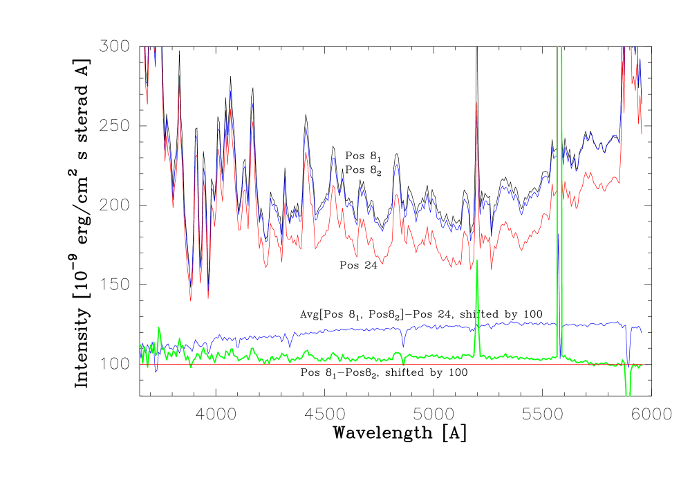
Figure 4: An example of the observing cycle ON-OFF-ON in the night 2004-09-18. The observed sky brightness spectra for the ON position (= Pos8) at the beginning and end of the cycle are shown as black and blue curves. Their difference, indicating the AGL variation during the cycle, is shown as the green curve with its zero point shifted by 100 $10^{-9}$ erg cm^-2s^-1sr^-1Å^-1 . The sky brightness spectrum for the OFF position (= Pos24) is shown as the red curve. The difference of the mean of the two ON spectra and the OFF spectrum is shown as the blue curve in the bottom part of the figure, with its zero point shifted by 100 $10^{-9}$ erg cm^-2s^-1sr^-1Å^-1 . Notice that the AGL variability was relatively low during this night as demonstrated by the small values of the ’quasi-continuum’ difference spectrum. However, the 520.0 Ni, 557.7 Oi and 589.0/589.6 nm NaD lines showed, as usual, a strong variability. The spectra are smoothed, wavelength bin is $\sim$0.7 nm and resolution $\sim$1.1 nm. Notice that while the difference spectrum of the two Pos8 observations (green line) still shows substantial residuals of the strong airglow features, they have almost completely disappeared in the Avg$[$Pos8₁,Pos8${}_{2}]$–Pos24 spectrum thanks to a linear variability with time of the airglow during this observation. All spectra in this figure are calibrated but not corrected for extinction and other atmospheric effects, i.e. they refer to the ground level.

4.2 Instrumental setup

In order to detect the Fraunhofer absorption line signature of the scattered light component and to separate it thereby, a spectral resolution of $R\ga 400$, or $\Delta\lambda\la 1$ nm, is needed. Our goal is to measure sky brightness differences (ON minus OFF) with a precision of $\sim$0.5 $10^{-9}$ erg cm^-2s^-1sr^-1Å^-1  or $\sim$0.2% of the dark sky brightness, which is $\sim$(200–300) $10^{-9}$ erg cm^-2s^-1sr^-1Å^-1  in the blue band. Most of the measurements were carried out in Periods 72 (2003–2004) and 86 (2011–2012) with FORS2 at UT1. Some data were obtained in Period 82 with FORS1 at UT2.

The long slit spectrometer (LSS) mode was used with Grism 600B which gave a spectral coverage from 320 to 600 nm and a nominal resolution of $R=780$ or 0.075 nm pixel^-1 for 1-arcsec slit width. We used the 2-arcsec slit to enable enough light to pass through and still to have a sufficient spectral resolution of $R\approx 400$ corresponding to $\sim$1 nm at 400 nm. In Periods 72 and 86 the detector was a mosaic of two 2k$\times$4k MIT/LL CCDs and in Period 82 a mosaic of two blue optimised E2V CCDs. All observations were carried out in the Service Mode.

In the setup for Period 72 and with the integration time of $t_{\rm int}$ = 17 min we measured for dark sky brightness a mean count rate of typically $\sim$120 e^- and $\sim$35 e^- per $2\times 2$ read-out bin (0.15 nm $\times$ 0.252 arcsec) at $\lambda\geq 450$ nm and $\lambda\approx 380$ nm, respectively. The detector read-out noise was (1.8–3.6) e^-/bin and the dark current 1.5 e^-/bin. Along the 6.8 arcmin long slit we can form an average over 1600 bins (= 400 arcsec) and in the dispersion direction over 2 bins (= 0.3 nm) giving a total sky signal of 384 $10^{3}$ and 112 $10^{3}$ e^- and a photon noise of 620 and 335 e^- for $\lambda\geq 450$ nm and for $\sim 380$ nm, respectively. The corresponding read-out noise is 100–200 e^- while the noise caused by the dark current is negligible. The total noise is thus $\la 650$ e^- (corresponding to 0.4 $10^{-9}$ erg cm^-2s^-1sr^-1Å^-1 ) and $\la$390 e^- (corresponding to 0.9 $10^{-9}$ erg cm^-2s^-1sr^-1Å^-1 ) at $\lambda\geq 450$ nm and at $\sim 380$ nm, respectively, corresponding to $\sim$0.2–0.3% of the sky signal. In Periods 82 and 86 the integration time was shorter, 315–330 s, but each position was then observed three or more times, thus giving a similar photon noise as in the above estimate. The larger relative contribution of the read-out noise was compensated by the reduced effect of airglow variations thanks to the shorter cycle time.

5 Data reduction

Data reduction was done using iraf (Image Reduction and Analysis Facility) (Tody, 1993). The details of the data reduction are the following.

5.1 Bias subtraction

The bias signal was determined by using the overscan regions of the detector. We determined for each of the two halves of the detector, Chip 1 and Chip 2, the mean values for each pixel column over the available $\sim$50 (Chip 1) and $\sim$250 (Chip 2) rows in the overscan region. These mean values were fitted with up to 5th degree Legendre polynomials and the resulting fitted values were subtracted from the pixel values in each column.

5.2 Wavelength calibration and correction for geometrical distortion

We corrected for geometrical distortion of the spectra in the following way in iraf: i) on a 2D arc-lamp spectrum the emission features along a single dispersion line are identified with the identify task of iraf; ii) the emission features at other dispersion lines are re-identified with the reidentify task; iii) the wavelengths of the identified features as a function of pixel position are fitted with a two-dimensional function using the fitcoords task; iv) the geometrical correction is made with the transform task, after which the wavelength is a linear function along one axis (dispersion is constant). Despite this correction, subtracting the background sky emission produces artefacts at the edges of the brightest airglow emission line profiles where the intensity gradient is steepest.

5.3 Extraction of the surface brightness signal

In each wavelength bin of 0.15 nm width the mean value was formed along the whole spatial extent of the slit, separately for the two halves of the detector, Chip 1 and Chip 2. The slit positions were generally chosen to be free of stars and galaxies to the limit of the DSS images. An exception was made for the Pos 42 spectra with slit position angle of 150°: the slit was intentionally positioned to pass over a faint star for the purpose of checking the coordinate setting accuracy and faint-star elimination procedure.

To eliminate the signal from faint stars and galaxies beyond the DSS limiting magnitude we used the idl sigma-clipping method. This method also eliminated the pixels with cosmic ray hits. The limit above or below of which the pixels were excluded was set to 3$\sigma$ where $\sigma$ is the standard deviation of the pixel values along the slit at a given wavelength. This standard deviation is determined mainly by the photon statistics and depends on the wavelength and the integration time. Applying the 3$\sigma$ cutting meant that, for the spectra with an integration time of 330 sec, the pixels with surface brightness in the $B$ band in excess of $\sim$140 $10^{-9}$ erg cm^-2s^-1sr^-1Å^-1  were excluded. For the integration time of 1042 s the 3$\sigma$ limit was $\sim$80 $10^{-9}$ erg cm^-2s^-1sr^-1Å^-1 . These cut-off limits correspond to outside-the-atmosphere $B$ band surface brightnesses of $\sim$23.3 and $\sim$23.9 mag/$\sq\arcsec$, respectively.

6 Calibration of surface brightness measurements

6.1 Special aspects of surface brightness calibration

The calibration of (spectro)photometry of extended uniform surface brightness differs from point-source photometry in the sense that one requires knowledge of two additional aspects: (1) the solid angle subtended by the spectrometer or photometer aperture or CCD detector pixel, and (2) the aperture correction factor.

Normally, the aperture correction factor, $T(A)$, is the fraction of the flux from a point source that is contained within the aperture. The fraction $1-T(A)$ of the point-source flux is lost outside the aperture. In the measurement of a uniform extended source, the situation is different: the flux that is lost from the solid angle defined by the focal plane aperture is compensated by the flux that is scattered and diffracted into the aperture from the sky outside of the solid angle of the aperture. Therefore, the intensity of an extended uniform source in $10^{-9}$ erg cm^-2s^-1sr^-1Å^-1  is given by

$$I(\lambda)=\frac{S(\lambda)T(A)}{\Omega}C(\lambda),$$ (3)

where $C(\lambda)$ is the signal in instrumental units (count s^-1), $\Omega$ the solid angle of the aperture in steradians, and $S(\lambda)$ the sensitivity function in units of $10^{-9}$ erg cm^-2s^-1Å^-1/(count s^-1) determined from the standard-star observations.

6.2 Observations of spectrophotometric standard stars

As part of ESO’s service mode operations spectrophotometric standard stars were observed in the same night (or in some cases the next night) with the same spectrometer setup as the surface brightnesses. However, instead of the 2-arcsec LSS slit the 5-arcsec MOS slit was used. The stars taken from ESO’s list of spectrophotometric standards: were in the magnitude range $V=10.4-13.2$ mag. The measurements were made using Chip 1 of the mosaic CCD detector only. The calibration for Chip 2 was accomplished by scaling its surface brightness values to Chip 1 values.

A special calibration observation was carried out in the night 2011-11-18 using the faint spectrophotometric standard star C26202 of the HST CalSpec list ($V=16.5$ mag, $B=16.90$ mag, spectral type F8 IV). The purpose was to check whether any detector non-linearity or other effects appear at the faint signal levels. Two spectra were taken through the 2 arcsec, slit: one unwidened spectrum and another one widened by drifting the star with a uniform speed along the slit over a distance of 100 arcsec. The latter observation produced in the $B$–band a signal corresponding to a surface brightness of 22.65 mag/$\sq\arcsec$ or $\sim$240 $10^{-9}$ erg cm^-2s^-1sr^-1Å^-1, similar to the night sky brightness. The sensitivity derived from the un-widened C26202 spectrum was consistent with the standard star spectra observed in the 5 arcsec MOS slit and showed no colour–dependent sensitivity difference. The sensitivity ratio derived from the widened and un-widened C26202 spectra was unity within $\pm$2% between 420 and 600 nm, but rose from 420 nm towards ultraviolet, reaching a value of 1.17 at 370 nm.

6.3 Atmospheric extinction corrections

Atmospheric extinction corrections were applied to the standard star flux values before using them for the calibration of the observed below-the-atmosphere night sky surface brightnesses. The average extinction coefficients as a function of wavelength for La Silla as measured in 1974-75 by Tüg (1977) were applied. The average extinctions for Paranal during 2008-09 in Patat et al. (2011) are slightly larger, by 0.02 to 0.04 mag per unit airmass between 350 and 600 nm. However, the average $UBVRI$ extinction coefficients reported by Patat (2003) for the period 03/2000 - 09/2001 are in good agreement with the La Silla values of Tüg (1977). Thus the La Silla values appear to be appropriate as mean extinction coefficients. They are close to the pure Rayleigh extinction coefficients for La Silla and Paranal.

The measured below-the-atmosphere surface brightness values were corrected to outside-the-atmosphere using the same extinction coefficients as for stellar photometry. This is justified by the fact that we are observing surface brightness differences over an area of at most a few degrees. Therefore, the aerosol scattering part of extinction which is removing photons from the line-of-sight beam is not compensated for by scattering back into the beam from the surrounding sky. This would be the case for much broader surface brightness distributions like that of the the ZL, extending over several tens of degrees on the sky.

The extinction coefficients vary from night to night. However, since both the standard stars and the surface brightness target positions were observed at small airmasses ($<1.25$) the night-to-night variations of the extinction coefficients have only minor influence. For example, for a deviation of the true extinction coefficient from the mean value of 0.41 mag/airmass at 370 nm by 0.05 mag/airmass the intensity error introduced is $<1.2$% if the standard star is at airmass 1.0 and the target at 1.25 or vice versa. Similar or smaller errors are obtained at other (longer) wavelengths. The errors of calibration stars’ extinction correction has only a minor effect on the final results, see Section 8.2.

6.4 Aperture correction

The standard star spectra were extracted from a stripe with a width of typically 10 pixels $(2\times 2)$ or 2.5 arcsec, corresponding to the core part of the PSF of the star image. In order to estimate the fraction of energy in the standard star’s image which falls outside of this 2.5 arcsec strip in the spatial direction and outside of the 5 arcsec slit in the dispersion direction we have stacked 17 standard star observations from all nights in Period 72. In this stacked image the star’s PSF profile can be traced out to a distance of $\sim$25 arcsec. Assuming that the energy distribution in the star image is centrally symmetric we have estimated the energy falling outside of the $2.5\arcsec\times 5\arcsec$ extraction slot up to a distance of 20 arcsec, separately for three wavelength ranges, 350–425, 425–500, and 500–600 nm. No wavelength dependence was found and the mean value and its mean error extracted from these three wavelength slots was $0.143\pm 0.006$. The seeing during the standard star observations was mostly $\leq 1.5$ arcsec, and thus its variations did not influence the fractional energy outside of $2.5$ arcsec. For the surface brightness measurements the seeing does not matter.

The part of energy falling outside of 20 arcsec was estimated in two steps: (1) for the range $100\arcsec-1400\arcsec$ we have made with VLT-UT2/FORS1 LSS spectrophotometric measurements of the star aureole using Sirius as light source (see Appendix B). With $I_{\rm stray}(r)$ the stray-radiation intensity, and $r$ the angular distance from the star the relationship log $I_{\rm stray}(r)$ vs. log $r$ was found to be closely linear with a slope of $\sim$-1.99. Thus we extrapolated the relation up to 2°  and found that within the range of 100″– 2°  the energy fraction was 0.038, closely the same in blue and visual. (2) An interpolation between the two sets of measurements gave an energy fraction of 0.029 between 20 and 100 arcsec. With an estimated uncertainty of $\pm 50$% for the energy fractions between 20″– 100″  and 100″– 2° , the total error was estimated to be $\sim\pm 0.05$. Summing up, we found that the total fraction of star flux lost was $1-T(A)=0.21\pm 0.05$ and the aperture correction factor was found to be $T(A)=0.79\pm 0.05$.

6.5 Width of the slit

The width of the slit used for the surface photometry was during all three periods $2.00$ arcsec and has an uncertainty of $\pm 0.02$ arcsec as given in the FORS1/2 Commissioning Report (non-public extensive version, M. van den Ancker, private communication 2014). The solid angle corresponding to one read-out pixel of $0.252$ arcsec in the spatial direction, i.e. the area of $0.252\arcsec\times 2.00\arcsec$, was thus $\Omega=(1.185\pm 0.01)\cdot 10^{-11}$ sterad.

7 Differential corrections for Zodiacal Light, Atmospheric Diffuse Light and straylight from stars

As explained in Section 2 the atmospheric, interplanetary and Galactic night sky components originating closer to us than the dark cloud are eliminated; this is true as long as they are constant over the area covered by our target positions and the duration of the ON–OFF–ON cycle. We need to consider only the differential effects caused by their time variation and the spatial differences over $\la$2$\aas@@fstack{\circ}$5. For the two IN-cloud positions, Pos9 and Pos42, the angular distance to the standard position was small enough, $\sim$10 arcmin, to, make such corrections superfluous.

The total diffuse sky brightness observed at a transparent OFF-position (= PosN) at airmass $X$ is given by

$$I^{X}_{\rm obs}{\rm(PosN)}=I_{\rm ZL}{\rm(PosN)}e^{-\tau(\lambda)X}+I^{X}_{\rm ADL}$$ (4)

where $I_{\rm ZL}$ is the ZL intensity outside the atmosphere and $\tau(\lambda)$ is the extinction coefficient. The ADL intensity, $I^{X}_{\rm ADL}$, is the sum the AGL and the three tropospheric scattered light components created by AGL, ZL and ISL as sources of light

$$I^{X}_{\rm ADL}=I^{X}_{\rm AGL}+I^{X}_{\rm SCA}({\rm AGL})+I^{X}_{\rm SCA}({\rm ZL})+I^{X}_{\rm SCA}({\rm ISL})$$ (5)

For the ON-position (= Pos8), observed at the slightly different airmass of $X+\Delta X$, the total diffuse light intensity is

$$I^{X+\Delta X}_{\rm obs}{\rm(Pos8)}=I_{\rm ZL}{\rm(Pos8)}e^{-\tau(\lambda)(X+\Delta X)}+I^{X+\Delta X}_{\rm ADL}+{}$$ (6)

$${}+\Delta I^{0}{\rm(Pos8-PosN)}e^{-\tau(\lambda)(X+\Delta X)}$$

where $\Delta I^{0}{\rm(Pos8-PosN)}$ is the (extraterrestrial) excess surface brightness of Pos8 relative to the transparent OFF position (PosN) outside the cloud. This is the quantity (spectrum) we want to derive for the several OFF positions.

The observed sky brightness difference between the ON and OFF position is thus given by:

$$\Delta I_{\rm obs}{\rm(Pos8-PosN)}=\Delta I^{0}{\rm(Pos8-PosN)}e^{-\tau(\lambda)(X+\Delta X)}+$$

$$+[I_{\rm ZL}{\rm(Pos8)}e^{-\tau(\lambda)(X+\Delta X)}-I_{\rm ZL}{\rm(PosN)}e^{-\tau(\lambda)X}]+$$

$$+[I^{X+\Delta X}_{\rm ADL}-I^{X}_{\rm ADL}]$$ (7)

The individual correction terms for the ZL and ADL are described in Appendix A. The corrections turn out to be $\sim$ 1 to 3 $10^{-9}$ erg cm^-2s^-1sr^-1Å^-1. To some extent they have for the individual OFF positions opposite sign and cancel out in the mean values.

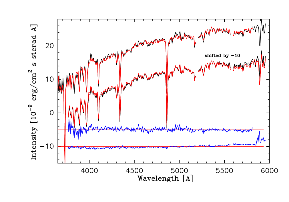
Figure 5: The observed surface brightness spectra for Pos8, $\Delta I^{0}$(Pos8–OFF), i.e. the difference relative to the average surface brightness of several OFF positions around the cloud. The two curves ’shifted by -10 units’ display the two ’Master mean’ spectra, using either method A (black curve) or method B (red curve) for the atmospheric diffuse light (ADL) correction. Their difference is shown as the bottommost blue curve with zero level indicated as red line. For the extreme red end, $\lambda=582-595$ nm, only the results for one OFF position (Pos20) in the exceptionally quiescent night 2010-12-14 are included. The ’Secondary mean’ spectrum is shown as the uppermost red curve. The topmost black curve is the mean of the two ’Master’ spectra, methods A and B. The difference of the ’Master’ and ’Secondary’ mean spectra is shown as the upper blue curve, with the zero level indicated as red line. The spectra have been smoothed with a 5-pixel boxcar function and have a bin size of $\sim$0.7 nm and a resolution of $\sim$1.1 nm. The spectra have gaps at the strong airglow lines at 520.0 and 557.7 nm. For the purpose of demonstrating the presence of the [Oii] 372.8 nm line and in order to avoid confusion the wavelength section 365–380 nm is shown for the upper two spectra only. The spectra have been corrected for extinction and other atmospheric effects, i.e. they refer to outside-the-atmosphere.

The surface brightness observed towards blank areas of sky, even if devoid of any resolved stars or galaxies, still contains instrumental straylight from stars that are outside of the observed area. Depending on their brightness stars up to several tens of arcminutes away can have a substantial straylight contribution. We have measured the straylight with FORS1 at UT2 over the angular offset range of $r$ = 100″–1400″ . The results are presented in Appendix B for several wavelength slots between 360 and 580 nm. These straylight profiles were used to calculate the $B$– and $V$–band straylight intensities for each target position. The straylight corrections are given in Table B1; they are small enough to be neglected in the further analysis. No differential straylight corrections are needed for Pos9 and Pos42, either.

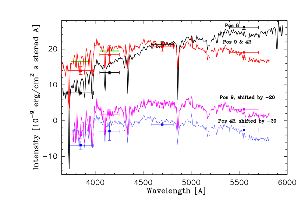
Figure 6: The observed surface brightness spectra for positions 8, 9 and 42, $\Delta I^{0}{\rm(Pos8-OFF)}$, $\Delta I^{0}{\rm(Pos9-OFF)}$, and $\Delta I^{0}{\rm(Pos42-OFF)}$. The black curve shows the overall mean for Pos8, including both the ’Master A&B mean’ and ’Secondary mean’ spectra with weights of 0.4 and 0.6, respectively. The spectra for Pos9 and Pos42 are shown as magenta and blue curves, with their zero point shifted by -20 units. The mean of the Pos9 and 42 spectra with weights 1 and 2.5, respectively, is shown as the red curve and is labelled as ’Pos 9 & 42’. The average fluxes of the ’Pos 9 & 42’ spectrum between 375 and 395 nm and between 405 and 425 nm are indicated with green bars; they are used for the determination of the 400 nm break strength. The spectra have been smoothed with a 5-pixel boxcar function and have a bin size of $\sim$0.7 nm and a resolution of $\sim$1.1 nm. The spectra have gaps at the strong airglow lines at 520.0 and 557.7 nm. The intermediate band photometric measurements (see Appendix C) are shown with the same colour coding as the spectra. The filter half-widths and the photometric (statistical) standard errors are indicated with horizontal and vertical bars. For the purpose of demonstrating the presence of the [Oii] 372.8 nm line, in order to avoid confusion, the 365–380 nm section is shown only for the upper two spectra. The spectra have been corrected for extinction and other atmospheric effects, i.e. they refer to outside-the-atmosphere.

8 Resulting spectra

The observational result consists of the surface brightness spectra at the positions 8, 9, and 42: $\Delta I^{0}$(Pos8 – OFF), $\Delta I^{0}$(Pos9 – OFF), and $\Delta I^{0}$(Pos42 – OFF). These spectra represent the surface brightness difference relative to the OFF-positions 18, 20, 24, 25, 32, 34, and 36; see Tables 1 and 2. The results refer to the extinction-corrected, i.e. outside-the-atmosphere spectra. The spectra for the IN-cloud positions, Pos9 and Pos42, have been calculated as:
$\Delta I^{0}$(Pos9 - OFF) = $\Delta I^{0}$(Pos8 - OFF) - $\Delta I^{0}$(Pos8 - Pos9),
$\Delta I^{0}$(Pos42 - OFF) = $\Delta I^{0}$(Pos8 – OFF) - $\Delta I^{0}$(Pos8 - Pos42), where $\Delta I^{0}$(Pos8 - Pos9) and $\Delta I^{0}$(Pos8 - Pos42) are the differential spectra w.r.t. Pos8 as obtained from observations and corrected for extinction only (see Section 4.1). For $\Delta I^{0}$(Pos8 - OFF) the mean of the ’Master mean’ and “Secondary mean” spectra was used in this case.

The results for Pos8 are shown in Fig. 5 separately for the ’Master mean’ and ’Secondary mean’ spectra, as detailed in Table 2. Two different reduction methods for the ADL, methods A and B, as described in Appendix A.2.1 and A.2.2, respectively, have been applied to the ’Master spectra’. The resulting mean spectra are shown in Fig. 5 as the lower pair of black (method A) and red (method B) curves, ’shifted by -10 units’. Their difference is shown as the lowest blue curve with the zero level indicated as red line. The results for methods A and B are seen to agree very closely which makes us confident that the effects of the AGL temporal and ADL spatial variations have been satisfactorily accounted for.

For the red end of the spectra, at 582–595 nm, the results from only one night are included (Pos20, night 2010-12-14). Even in this quiescent night the variations of the atmospheric NaD line and the adjacent OH(8-2) bands cause in this wavelength slot a substantially larger disturbance than is elsewhere the case. However, the detection of the NaD absorption line in the $\Delta I^{0}$(Pos8 - OFF) spectrum is well secured.

The mean ’Secondary spectrum’, as described in Appendix A.2.3, is shown as the uppermost red curve in Fig. 5 together with the mean of the two (methods A and B) ’Master mean’ spectra (black curve). The difference between the two spectra is shown as the upper blue curve, with its zero level indicated as the red line.

An overall average of all Pos8 spectra, i.e. the mean of the ’Master A&B’ and the ’Secondary mean’ spectra is shown in Fig. 6 as the black curve. Before averaging, the ’Secondary mean’ spectrum was adjusted to the ’Master mean’ overall continuum by means of a 4^th degree polynomial fit. Thus, this spectrum has the same broad-band continuum as the ’Master mean’ spectrum but an improved S/N ratio, corresponding to the combined integration time of the ’Master’ and ’Secondary mean’ spectra.

The spectra for Pos9 and Pos42 are shown in Fig. 6 as the magenta and blue curves, with their zero point shifted by -20 units. The weighted mean of Pos9 and Pos42 spectra (weights 1 and 2.5) is shown as the red line labelled with ’Pos 9 & 42’.

An inspection of the spectra reveals the following salient features which reflect the fact that the spectra are dominated by the scattered light from the all-sky ISRF plus the line emission from ionized gas in the cloud area:
(i) the spectra show strong Fraunhofer lines: Caii H (396.8 nm, blended with H $\epsilon$), Caii K (323.3 nm), G band (430.0 nm), Mgi+MgH (518.0 nm), the Balmer H $\beta$ (486.1 nm), H $\gamma$ (434.1 nm), H $\delta$ (410.3 nm);
(ii) the 400 nm break, present in the integrated spectra of galaxies, is also clearly visible in our scattered light spectra. The break strength, $D(4000)$, is defined as the ratio of the average flux density between 405 and 425 nm to that between 375 and 395 nm (Bruzual A., 1983), where the flux density is in units of erg s^-1cm^-2Hz^-1. For the ’Pos 9&42’ spectrum the mean flux densities in the two reference intervals are 19.5 and 16.5 $10^{-9}$ erg cm^-2s^-1sr^-1Å^-1, and are indicated with green bars in Fig. 6. (In determining these mean fluxes we have taken into account the small contribution by the LOS Balmer line emission of ionised gas, see Paper II, Section 2.1.3.) Transforming the flux densities to erg s^-1cm^-2Hz^-1 units their ratio is $D(4000)\approx 1.4$. This is at the lower end of the range of $D(4000)$ values found for the total light of spiral galaxies (see e.g Bruzual A. 1983; Hamilton 1985; Dressler & Shectman 1987). This can be understood because our spectra represent the light from the outer parts of the Milky Way Galaxy with little contribution from the bulge component with its stronger 400 nm break. Because of the intermediate extinction towards Pos9 and Pos42 the overall spectral shape is closely similar to integrated starlight spectrum. For the strongly reddened Pos8 spectrum a similar $D(4000)$ strength is indicated, after the effect of reddening is accounted for.
(iii) the SED of Pos 8 is substantially redder as compared to the SEDs of Pos9, Pos42 and the all-sky ISL (see Fig. 2). Because of the large optical depth for Pos8 at all wavelengths the SED shape is dominated by effects of multiple scattering and absorption;
(iv) the lower optical depth for Pos42 ($A_{\rm V}=0.86$ mag) as compared to Pos9 ($A_{\rm V}=1.17$ mag) results in a lower surface brightness in visual and red, roughly proportional to their extinction ratio. At the blue end, because of saturation, the ratio is closer to 1;
(v) the Balmer lines, H $\beta$, H $\gamma$, and H $\delta$ are, especially for Pos8, stronger than expected for scattered starlight (compare also with Fig. 2). This indicates that there is a substantial excess of line emission by ionized gas from the OFF positions. This is also the cause for the strong [Oii] 372.8 nm line, seen as an apparent absorption line in these spectra.

The spectra as displayed in Fig. 6 are provided also as machine readable files, see Appendix D for explanations.

Table 3: Mean values and error estimates for selected wavelength intervals of the Pos8 and Pos42 spectra as specified in the text. The quantities given in the Table are: mean value = average surface brightness over the wavelength interval; $\sigma$(mean) = standard error of the mean value; $\sigma$(pix-to-pix) = pixel-to-pixel standard error for spectrum smoothed with 5-pixel boxcar function resulting in $\sim 0.7$ nm bins. The unit is $10^{-9}$ erg cm^-2s^-1sr^-1Å^-1.

		Wavelength interval [nm]
		————————————————————————————————–
		380-	385-	391-	401-	416-	438-	470-	494-	510-	534-	565-
		385	391	396	406	426	448	480	502	517	549	580
$\Delta I^{0}$(Pos8 - OFF)
’Master mean’, method A	mean	9.5	9.8	12.3	16.0	16.8	18.3	21.4	22.8	22.2	24.8	24.5
	$\sigma$(mean)	0.54	0.99	0.18	0.16	0.16	0.37	0.48	0.33	0.43	0.55	1.27
$\Delta I^{0}$(Pos8 - OFF)
’Master mean’, method B	mean	9.7	10.1	12.5	16.5	17.2	18.6	21.6	23.0	22.0	24.7	23.8
	$\sigma$(mean)	1.15	1.22	0.57	0.83	0.56	0.73	0.69	0.65	0.58	0.39	0.46
$\Delta I^{0}$(Pos8 - OFF), ’Master Mean’
$\Delta I^{0}$(method A)- $\Delta I^{0}$(method B)	$\Delta$(mean)	-0.2	-0.3	-0.2	-0.5	-0.4	-0.3	-0.2	-0.2	0.2	0.1	0.7
$\Delta I^{0}$(Pos8 - OFF)
$\Delta I^{0}$(’Master’) - $\Delta I^{0}$(’Secondary’)	$\sigma$(pix-to-pix)	1.32	1.15	0.79	0.45	0.40	0.33	0.38	0.60	0.41	0.18	0.28
$\frac{1}{2}[\Delta I^{0}$(’Master’)+$\Delta I^{0}$(’Secondary’)]	$\sigma$(pix-to-pix)	0.66	0.58	0.40	0.22	0.20	0.16	0.19	0.30	0.20	0.09	0.14
$\Delta I^{0}$(Pos42-Pos8)]
	$\sigma$(mean)	0.51	0.46	0.46	0.47	0.47	0.66	0.81	0.79	0.66	0.59	1.15
	$\sigma$(pix-to-pix)	0.54	0.41	0.51	0.26	0.42	0.38	0.34	0.51	0.35	0.48	0.40

Table 4: Summary of the sky background brightness components towards our target area: the Zodiacal Light (ZL), atmospheric diffuse light (ADL) that is the sum of Airglow (AGL) and tropospheric scattered light, the scattered light from the cloud, $\Delta I^{0}$(Cloud – OFF), for Pos8, Pos9 or Pos42, the the Diffuse Galactic Light (DGL) in the surroundings (OFF positions), and our measurement of the EBL. These values refer to the spectroscopic observations as listed in Table 2. Under ’differential corrections’ the ranges of the corrections $\Delta I_{\rm ZL}$, $\Delta I_{\rm ADL}$ and $\Delta I_{\rm stray}$ are given for the different Pos8 – OFF spectra listed in Table 2. A compilation of error estimates according to Table 3 and Sections 8.1 and 8.2 is included in the bottom part of the table. The calibration errors are in per cent. All values refer to outside the atmosphere, except for $I_{\rm ADL}$ which is the value below the troposphere, at ground-level.

Component	Wavelength	Value	Reference/Comment
	[nm]	[$10^{-9}$ erg cm-2s-1sr-1Å-1 ]
$I_{\rm ZL}$	500	102 – 105	Leinert et al. (1998)
$I_{\rm ZL}$	400 – 420	88 – 99	derived from $I_{\rm ZL}$ at 500 nm
$I_{\rm ADL}$	400 – 420	83 – 138	see Section 7, equation (5)
$\Delta I^{0}$(Cloud – OFF)	400 – 420	16 – 22	see Table 3
$I_{\rm DGL}$(OFF)	555	3.3	see Paper II, Section 2.1.2
$I_{\rm DGL}$(OFF)	400 – 420	4.6	see Paper II, equation (7)
$I_{\rm EBL}$	400	2.9	see Paper II
Differential corrections
$\Delta I_{\rm ZL}$	400 – 420	-2.7 – 3.5	see Table 2, Column (8)
$\Delta I_{\rm ADL}$	400 – 420	-1.8 – 1.8	see Appendix A2 and equation (A3)
$\Delta I_{\rm stray}$	400 – 500	-0.6 – 1.7	Appendix B, Table B1
Statistical errors
$\sigma$(pixel-to-pixel)	385 – 400	$\leq 0.6$	Section 8.1 and Table 3
$\sigma$(pixel-to-pixel)	400 – 500	$\leq 0.2$	Section 8.1 and Table 3
$\sigma$(mean)	350 – 500	$\leq 0.5$	Section 8.1 and Table 3
Calibration errors
$\sigma$(stars)		$\leq$ 7%	Section 8.2
$\sigma$(extinction)		$\leq$ 1.2%	Section 8.2
$\sigma$(aperture correction))		$\leq$ 6%	Section 8.2

8.1 Statistical errors

The statistical errors influencing the observed spectra are considered from two points of view:
(i) The pixel-to-pixel statistical error. It is mainly caused by the photon statistics and instrumental read-out noise; this noise is an important limiting factor for the determination of the Fraunhofer line depths and the 400 nm discontinuity, which are utilized for the evaluation of the scattered starlight contribution to the spectra.
(ii) The error in the zero level. Besides by photon statistics and read-out noise as in (i), it is caused also by the uncertainties of the differential ADL and ZL corrections.

For the ’Master mean’ spectrum the deviations of the four individual spectra from the mean have been used to estimate the statistical error of the zero level. In the first two parts of Table 3 the mean values and their mean errors, $\sigma$(mean), are given for selected wavelength intervals. The wavelength intervals are broad enough so that the $\sigma$(mean) values are dominated by the zero-level error and not the pixel-to-pixel noise. The mean values for methods A and B agree to within $\la$0.5 $10^{-9}$ erg cm^-2s^-1sr^-1Å^-1  (see third part of Table 3 and Fig. 5). This is consistent with the $\sigma$(mean) values that for method A are $\la$0.5 $10^{-9}$ erg cm^-2s^-1sr^-1Å^-1  over most of the wavelength range and it indicates that the differential ADL corrections do not introduce zero-level errors larger than this. The smaller $\sigma$(mean) values for method A as compared to method B indicate that the AGL time variations (whose influence is minimized in method A) are more important as an error source than the ADL zenith distance dependence (eliminated in method B).

The pixel-to-pixel noise cannot be directly determined from the mean spectra because of the intrinsic structures in the underlying scattered light (ISL) spectrum. We have therefore used the difference spectrum ’Master mean (A&B)’ minus ’Secondary mean’, $\Delta I^{0}{\rm(^{\prime}Master^{\prime})}-\Delta I^{0}{\rm(^{\prime}Secondary^{\prime})}$ (see Fig. 5) to derive the $\sigma$(pixel-to-pixel) values as listed in the fourth part of Table 3. Because the total integration times of the ’Master’ and ’Secondary mean’ spectra are similar, the noise for each of them is $\sim 1/\sqrt{2}$ times, and the noise for their mean is $\sim 1/2$ times the $\sigma$(pixel-to-pixel) noise of the difference spectrum. The $\sigma$(pixel-to-pixel) values for the mean are also given in part 4 of of Table 3.

The values of $\sigma$(mean) for the $\Delta I^{0}$(Pos42 - Pos8) spectrum (Table 3, Part 5) were derived from the deviations of the individual spectra from their mean. Since the contribution by the underlying spectral structure of the ISL spectrum turned out to be a minor factor compared to the other noise components, the $\sigma$(pixel-to-pixel) values of the $\Delta I^{0}$(Pos42 - Pos8) spectrum were directly adopted. For the error estimates of the mean of $\Delta I^{0}$(Pos9 - Pos8) and $\Delta I^{0}$(Pos42 - Pos8) we have adopted the values as derived for Pos42 because it dominates the mean by its larger weight (2.5 vs. 1).

In summary, the pixel-to-pixel statistical errors, important for the fitting accuracy (and elimination) of the scattered light spectrum, are $\la 0.6$ $10^{-9}$ erg cm^-2s^-1sr^-1Å^-1  for $\lambda<400$nm, and $\la 0.2$ $10^{-9}$ erg cm^-2s^-1sr^-1Å^-1  for $\lambda>400$ nm, respectively, as found for the mean of the ’Master’ and ’Secondary’ mean spectra. The accuracy of the zero level of the ’Master Mean’ spectrum can conservatively be estimated to be $\leq 0.5$ $10^{-9}$ erg cm^-2s^-1sr^-1Å^-1  for $\lambda\geq 390$nm as indicated by the $\sigma$(mean)$\leq 0.5$ $10^{-9}$ erg cm^-2s^-1sr^-1Å^-1  errors for the ’Master mean’ method A spectrum, and by the $\leq 0.4$ $10^{-9}$ erg cm^-2s^-1sr^-1Å^-1  differences between the ’Master mean’ method A and B spectra.

8.2 Calibration errors

Our observations are differential and the night sky component separation is carried out using data from the same telescope for all components. Therefore, unlike in the methods applied by Bernstein et al. (2002a) and Matsuoka et al. (2011), an absolute flux calibration of high accuracy is not required for the component separation. The calibration error appears essentially only as a scaling factor in the derived EBL value.

A source of calibration errors are the observations of standard stars, i.e. their pure observational errors, the photometric stability of the instrumental system over up to two days, and the transformation to the standard spectrophotometric system. For the service mode observations the VLT/FORS User Manual cites an accuracy of 10% for an individual night. For our Master mean’ and ’Secondary mean’ spectra, which combine averages of three or six nights, respectively, we somewhat arbitrarily estimate that this error is reduced to $\la$7%.

The error caused by uncertainties of extinction correction has been estimated to be $<1.2$% (see Section 6.3).

In addition, there are the errors caused by the specific aspects of extended surface brightness calibration. These are the errors for the spectrometer solid angle $\Omega$ of $\pm 1$%, and of the aperture correction factor $T(A)$ of $\pm 6$%, as discussed in Sections 6.4 and 6.5.

A quadratic addition of the standard star photometric, the extinction, and the aperture correction factor errors gives the overall calibration error estimate of $\la\pm 9$%.

For comparison, we show in Fig. 6 also results of the intermediate band photometry (see Appendix C). The agreement between the spectroscopic and photometric values is within the $\la\pm 9$% calibration uncertainty.

8.3 Summary of sky components, differential corrections and errors

We summarise in Table 4 the contributions of the sky surface brightness components valid for the sky area and time slots of our spectroscopic observations: the Zodiacal Light, Atmospheric Diffuse Light and Diffuse Galactic Light. For comparison, the surface brightness excess of the positions 8, 9 and 42 in L 1642 and our result for EBL intensity are given. The range of values of the small differential corrections caused by the ZL, ADL and instrumental straylight are listed next; we refer to the detailed description of these corrections in Section 7, Appendix A and B. In the mean spectrum, $\Delta I^{0}$(Pos8 – OFF), the corrections with opposite signs cancel out partly.

In the lower part of the table we summarise the errors; the detailed description of them is given in Sections 8.1 and 8.2.

The general DGL, i.e. the scattered light from dust in the surroungs of the cloud, has been estimated using the mean extinction for the OFF positions , $A_{\rm V}\approx 0.15$ mag (see Section 3 and Table 1). Using the relationship between the optical extinction and 200 $\mu$m surface brightness on the one, and that between the optical and 200 $\mu$m surface brightnesses on the other side (see Appendix C) this $A_{\rm V}$ value is found to correspond to a DGL value of $I_{\rm DGL}=3.3$ $10^{-9}$ erg cm^-2s^-1sr^-1Å^-1  at $\lambda=555$ nm. For details, see Paper II, Section 2.1.2.

9 Summary and Conclusions

We utilize the shadowing effect of an opaque dark cloud to measure the EBL plus possible other diffuse light components originating from beyond the cloud. However, besides screening background light the dark cloud also scatters light from the all-sky Interstellar Radiation Field (ISRF, consisting mainly of ISL) into the line of sight. In order to separate the EBL and ISL components we utilize the fact that their spectra are different: smooth continuum (EBL) vs. line spectrum (ISL). The component separation and results for the EBL are presented in the accompanying Paper II (Mattila et al., 2017b).

In this paper we have presented spectrophotometric measurements of the faint surface brightness in the area of the high galactic latitude dark cloud Lynds 1642. The cloud has a high opacity core with $A_{\rm V}\ga 15$ mag, blocking the EBL almost completely, while there are ’clear’ areas within 2$\aas@@fstack{\circ}$5 from the cloud core with good transparency ($A_{V}\approx 0.15$ mag). We have presented a spectrum for the difference ’opaque core minus clear sky’. In addition, two intermediate opacity positions, $A_{\rm V}\approx 1$ mag, have been observed and their spectra ’cloud minus clear sky’ will be utilized in Paper II to facilitate the separation of the ISL and EBL light components. Because of the pseudosimultaneous differential measurements the spectra are virtually free of the large foreground atmospheric and Zodiacal Light components.

For the separation of EBL and scattered ISL a spectral resolution of $R\sim 400$ is required and was achieved with long slit spectroscopy with VLT/FORS. A precision of $\sim$ 0.5 $10^{-9}$ erg cm^-2s^-1sr^-1Å^-1  was achieved for the averaged differential spectrum ’cloud core minus clear sky’. Such a precision is required for the study of the EBL signal which is in the range of 1 to a few times $10^{-9}$ erg cm^-2s^-1sr^-1Å^-1 . In the dark cloud method all diffuse light components are measured using the same equipment, and the component separation is done before the calibration. Thus, we do not need an unusually high absolute calibration accuracy as is the case for projects in which the small EBL signal has to be derived as the difference of $\sim$50 to 100 times larger surface brightness signals.

An inspection of the spectra (see Fig. 6) reveals the following salient features which reflect the fact that the spectra are dominated by scattered light from the all-sky ISRF plus line emission from ionized gas in the cloud area: (i) the spectra show distinctly the strong Fraunhofer lines: Caii H (blended with H$\epsilon$), Caii K, G band, Mgi+MgH, the Balmer H $\beta$, H $\gamma$, H $\delta$, and the 400 nm discontinuity, typical of integrated spectra of late type spiral galaxies; (ii) the SED of the opaque core is substantially reddened as compared to the SEDs of the intermediate opacity positions and the ISL. Because of the large optical depth of the core the SED shape is dominated by effects of multiple scattering and absorption; (iii) the Balmer lines are stronger than expected for scattered starlight. This indicates that there is a substantial excess of line emission by ionized gas from the OFF positions. This is also the cause for the strong [Oii] 372.8 nm line, seen as an apparent absorption line in these spectra. On the other hand, [Oiii] 500.7 nm is seen as an emission line indicating that it originates mainly as scattered light from the all-sky ISRF.

The separation of the EBL from the scattered light of the dark nebula is described in the accompanying Paper II (Mattila et al., 2017b). As template for the scattered starlight spectrum we make use of the spectra at the two semi-transparent positions 9 and 42. The main results are: The EBL intensity at 400 nm is $I_{\rm EBL}=2.9\pm 1.1$ $10^{-9}$ erg cm^-2s^-1sr^-1Å^-1  or $11.6\pm 4.4$ nW m^-2sr^-1, which represents a 2.6$\sigma$ detection; the scaling uncertainty is +20%/-16%. At 520 nm we have set a 2$\sigma$ upper limit of $I_{\rm EBL}\leq$4.5 $10^{-9}$ erg cm^-2s^-1sr^-1Å^-1  or $\leq$ 23.4 nW m^-2sr^-1 +20%/-16% . Our EBL value at 400 nm is $\ga 2$ times as high as the integrated light of galaxies. No known diffuse light sources, such as light from Milky Way halo, intra-cluster or intra-group stars appear capable of explaining the observed EBL excess over the integrated light of galaxies.

Besides the main purpose, i.e. the EBL determination, the resulting spectra of the present paper can also be used for two other purposes: (i) determination of the scattering properties of dust, namely the albedo and the asymmetry parameter as function of wavelength (see e.g. Mattila 1970; Laureijs, Mattila, & Schnur 1987), and (ii) empirical test of the synthetic spectrum of the Solar neighbourhood ISL (see Paper II, Appendix A). Concerning the latter application we note especially that the dark cloud ’sees’ the Milky Way from a vantage point that is $\sim$ 85 pc off the galactic plane.

Appendix A Differential corrections for Zodiacal Light and Atmospheric Diffuse light

A.1 Differential Zodiacal Light correction

With the designation $\Delta I_{\rm ZL}=I_{\rm ZL}({\rm Pos8})-I_{\rm ZL}({\rm PosN})$ the ZL correction term in equation (7), reduced to outside the atmosphere, can be expressed as:

$$\Delta I^{\rm{\rm corr}}_{\rm ZL}=$$

$$=[I_{\rm ZL}{\rm(Pos8)}e^{-\tau(\lambda)(X+\Delta X)}-I_{\rm ZL}{\rm(PosN)}e^{-\tau(\lambda)X}]e^{\tau(\lambda)X}$$

$$=\Delta I_{\rm ZL}-\Delta X\tau(\lambda)I_{\rm ZL}$$ (8)

where the term $\Delta X\tau(\lambda)I_{\rm ZL}$ accounts for the slightly different atmospheric extinctions for the Pos8 and PosN observations. With the ecliptic coordinates $\lambda-\lambda_{\sun}$ and $\beta$ given for the observed ON and OFF positions at each observing date, we have interpolated from Table 17 of Leinert et al. (1998) the mean ZL intensity for Po8 and PosN, $I_{\rm ZL}$, and the difference $\Delta I_{\rm ZL}$. Their values at $\lambda=500$ nm are given in column (8) of Table 2. While the absolute ZL intensities are known only to an accuracy of $\sim 10$ $10^{-9}$ erg cm^-2s^-1sr^-1Å^-1  (Leinert et al., 1998) the differences $\Delta I_{\rm ZL}$ over separations of a few degrees are more accurate, of the order of a few tenths of $10^{-9}$ erg cm^-2s^-1sr^-1Å^-1 , as estimated from Table 16 of Leinert et al. (1998).

In order to estimate $I_{\rm ZL}(\lambda)$ and $\Delta I_{\rm ZL}$ at other wavelengths than 500 nm we adopt as starting point the Solar spectrum as given by Kurucz et al. (1984) (in digital form at http://kurucz.harvard.edu/sun.html). To account for the redder colour of the ZL as compared to the Sun we multiply the Solar spectrum with the correction factor $f_{\rm co-90}$ as given by equation (22) in Leinert et al. (1998). For the wavelength range $\lambda=360-580$ nm it can be satisfactorily represented by: $f_{\rm co-90}(\lambda)=1.0+0.74\cdot 10^{-3}(\lambda-500$ nm). The solar and the ZL spectra are rather similar to the ISL spectrum. Therefore, the ZL correction is partly ’absorbed’ into the scattered ISL component and its uncertainty is not causing an error in the EBL value with full weight (see Paper II).

A.2 Differential Atmospheric Diffuse Light correction

The AGL and atmospheric scattered light cause both random and systematic variations of the sky brightness. The random effects consist of
(i) temporary variations of the AGL on time scales of $\sim$10 minutes to hours, and
(ii) irregular (’cloudy’) spatial variations of the AGL on scales from several degrees upwards.
The systematic effect consists of
(iii) the zenith distance dependence of AGL and tropospheric scattered light, jointly called atmospheric diffuse light, ADL.

For the ADL correction of the ’Master spectra’ we have used two independent complementary methods.

A.2.1 Method A that minimizes the effect of AGL time variations

The observations in the cycle Pos$8_{1}$ - PosN - Pos$8_{2}$ are equally spaced in time. The airglow time variations are thus eliminated as long as they are linear in time, and the error introduced by the non-linearity is expected to be substantially smaller than $|I_{1}(Pos8)-I_{2}(Pos8)|$. However, because the three observations, Pos$8_{1}$, PosN, and Pos$8_{2}$, are taken at slightly different zenith distances, a systematic effect is caused by the zenith distance dependence of the ADL.

Near the zenith the atmosphere can be approximated as plane parallel, and at airmasses $X\la 1.3$ the ADL intensity can be given by

$$I^{\rm X}_{\rm ADL}=I^{X}_{\rm AGL}+I^{X}_{\rm SCA}=I^{1.0}_{\rm ADL}[1+k(\lambda)(X-1)]$$ (9)

where $I^{1.0}_{\rm ADL}$ is the ADL intensity in zenith ($X=1.0$). The ADL difference between airmasses $X+\Delta X$ and $X$ is thus given by

$$\Delta I^{X+\Delta X,X}_{\rm{ADL}}={\scriptstyle\frac{k(\lambda)}{1+k(\lambda)(X-1)}}\Delta X\cdot I^{X}_{\rm{ADL}}=C(\lambda)\cdot\Delta X\cdot I^{X}_{\rm ADL}$$ (10)

where $C(\lambda)=k(\lambda)[1+k(\lambda)(X-1)]^{-1}$. We have determined the values of $k(\lambda)$ and $C(\lambda)$ using the tables of Ashburn (1954) that are based on the solution of the multiple scattering problem in plane parallel atmosphere using the Chandrasekhar-formalism (Chandrasekhar, 1950). The Ashburn tables give the combined AGL and tropospheric scattered light at ground for different extinctions and AGL layer heights. The case of infinite layer height can be used for modelling the scattered light from extraterrestrial light sources. Combining the results for the layer heights of 100 km (AGL) and $\infty$ (ZL and ISL) we obtained the values $k(\lambda)$ = 0.65, 0.70, 0.75, 0.80, 0.85 and $C(\lambda)$ = 0.61, 0.65, 0.70, 0.74, 0.78 at $\lambda$ = 360, 400, 450, 500 and 550-600 nm, respectively. The values of $C(\lambda)$ are for an airmass of 1.10, representative for the ’Master spectra’.

Using equation (4) we obtain for the ADL correction, referred to outside the atmosphere, the expression

$$\Delta I_{\rm ADL}^{\rm corr}=[I^{X}_{\rm obs}-I_{\rm ZL}e^{-\tau(\lambda)X}]C(\lambda)\Delta Xe^{\tau(\lambda)X}$$ (11)

Applying the differential ADL and ZL corrections, the outside-the-atmosphere ON minus OFF surface brightness difference is then given according to equation (7)

$$\Delta I^{0}{\rm(Pos8-PosN)} = \Delta I_{\rm obs}{\rm(Pos8-PosN)}e^{\tau(\lambda)X}-$$ (12)

$$- \Delta I_{\rm ADL}^{\rm corr}-\Delta I_{\rm ZL}^{\rm corr}$$

We give in column (7) of Table 2 for each measurement the airmass for the OFF position (PosN) and the airmass difference $\Delta X=X$(Pos8) - $X$(PosN). For airmass differences of $\Delta X=$ -0.034 to +0.032 the corrections $\Delta I^{X,X+\Delta X}_{\rm ADL}$ range from -1.8 to +1.8 $10^{-9}$ erg cm^-2s^-1sr^-1Å^-1. The correction for the ’Master mean’ spectrum is +0.8 $10^{-9}$ erg cm^-2s^-1sr^-1Å^-1.

A.2.2 Method B that avoids the effect of ADL zenith distance dependence

We have used also another reduction method in which the ADL zenith distance dependence does not enter. In the measuring cycle Pos8₁ - PosN - Pos8₂ the zenith distances for Pos8₁ and Pos8₂ bracket that of the PosN measurement. It is possible to choose the weights $w_{1}$ and $w_{2}$ in such a way that for the weighted mean $\overline{I{\rm(Pos8)}}=w_{1}I_{1}{\rm(Pos8)}+w_{2}I_{2}{\rm(Pos8)}$ the weighted airmass $\overline{X{\rm(Pos8)}}=w_{1}X_{1}{\rm(Pos8)}+w_{2}X_{2}{\rm(Pos8)}$ is equal to the airmass of the PosN measurement. The weights vary between 0.46/0.54 and 0.18/0.82. The observed surface brightness difference
$\Delta I_{\rm obs}{\rm(Pos8-PosN)}=\overline{I{\rm(Pos8)}}-I{\rm(PosN)}$ has to be corrected in this case for ZL only, and we have instead of equation (A5):

$$\Delta I^{0}{\rm(Pos8-PosN)}=\Delta I_{\rm obs}{\rm(Pos8-PosN)}e^{\tau(\lambda)X}-\Delta I_{\rm ZL}$$

A drawback of this method is that the elimination of the AGL time variations is less optimal.

We have applied both methods, A and B, to the correction of “Master spectra”. The results are presented in Section 8 and Fig. 5.

A.2.3 ADL correction for the ’Secondary spectra’

For the ’secondary spectra’ the AGL time variation was too large, $|I_{1}{\rm(Pos8)}-I_{2}{\rm(Pos8)}|>5$ $10^{-9}$ erg cm^-2s^-1sr^-1Å^-1 , to enable an independent accurate extraction of the differential spectra $\Delta I_{\rm obs}$(Pos8 – PosN). Using Method A as described above the resulting spectrum still contained a substantial residual component of the AGL which had not been removed by the linear interpolation. We can assume, however, that the spectral form of this residual AGL component is well approximated by the spectrum of the difference signal between the two consecutive observations of the same position, $\Delta I_{\rm AGL}$(Pos8_1-2) = $I_{1}$(Pos8) – $I_{2}$(Pos8). Thus, we have added to the spectrum $\Delta I_{\rm obs}$(Pos8 – PosN) a suitable fraction, $-0.5<F<0.5$, of the differential AGL spectrum so that the resulting corrected spectrum

$$\Delta I^{0}{\rm(Pos8-PosN)}={}$$ (14)

$${}=\Delta I_{\rm obs}{\rm(Pos8-PosN)}+F\cdot\Delta I_{\rm AGL}{\rm(Pos8}_{1-2})$$

is optimised in two ways: (i) it fits as well as possible to the mean of ’Master spectra’, and (ii) the residual contributions of the AGL emission bands as seen in the difference spectrum $\Delta I_{\rm AGL}{\rm(Pos8}_{1-2})$ are minimised. We notice that this correction procedure does not influence the strengths of the non-AGL related features in the $\Delta I_{\rm obs}{\rm(Pos8-PosN)}$ spectrum. Since the mean ’Secondary spectrum’ is mainly used to improve the S/N ratio, we adjust, as a final step, its continuum level by a polynomial fit to the mean ’Master spectrum’. For the result see Section 8 and Fig. 5.

Appendix B Instrumental straylight

B.1 Measurement of straylight profile of a star

The stray radiation profile of a star, $I_{\rm stray}(r)$, in the range of $r\approx 1$ arcmin – 1 deg is thought to be caused mainly by scattering from the telescope main mirror micro-ripple and dust contamination (see e.g. Beckers 1995).

Using the same LSS setup with FORS1 at UT2 as described in Section 4.2 we have measured the straylight over 360 - 580 nm. The measurements were made on 2009-01-26 using Sirius as light source. The angular range of $r$ = 100″- 1400″  was covered with three slit positions, 45″  East of Sirius, oriented along the N-S direction: $r$ = $\sim$100″  – 500″  South; $\sim$400″- 800″  North; and $\sim$1000″  – 1400″  South. As zero level we used spectra taken symmetrically at 2°  North and South. Integration time was 255 s and airmass 1.0. The data reduction and calibration were performed as described in Sections 5 and 6. The scaling of the middle region was adjusted slightly ($\sim 12\%$) to make it fit smoothly to the innermost region in the overlapping part at 400″  - 500″  and, correspondingly, the outermost region was adjusted to the middle region (by $\la 10\%$) to provide a smooth continuation over the gap from $\sim$800″  to 1000″ . The closely linear form of    log$I_{\rm stray}(r)$ vs. log$r$    enabled a safe interpolation over 800″- 1000″  as well as the the small gaps between Chip 1 and 2. Spikes by stars were removed by interpolation of the intensity over such locations. Finally, the straylight spectra were divided by the spectra of Sirius, adopted from Kurucz et al. (1984), convolved to the resolution of our straylight spectra, and extinction corrected to below the atmosphere.

We show in Fig. B1 the straylight intensity $I_{\rm stray}(r)$ as function of offset from Sirius, $r$, for four wavelength slots, $\lambda=360-380$ nm, $400-420$ nm, $480-500$ nm and $560-580$ nm. The observed straylight follows over the range 120″  - 1400″  the functional form according to King (1971), $I_{\rm stray}\propto r^{-2}$, with a slight upturn at $r<$120″ . For the wavelength bands $420-460$ nm and $480-520$ nm corresponding to the Tycho $B_{T}$ and $V_{T}$ magnitudes, we obtain the straight line fits:
log $I_{\rm stray}=-1.988(\pm 0.003){\rm log}r\arcsec-2.837(\pm 0.008)$ and
log $I_{\rm stray}=-1.985(\pm 0.004){\rm log}r\arcsec-2.879(\pm 0.012)$.
Our $I_{\rm stray}$ level at 420–460 nm is by $\sim$0.50 mag, i.e by a factor of $\sim$1.60 higher than the straylight profile of King, valid for the blue (photographic) band, shown in Fig. B1 for reference.

B.2 Straylight for observed positions

The straylight intensities were calculated in the $B_{T}$ and $V_{T}$ bands for each target position in the L 1642 cloud area. For stars with $B_{T}\leq 12.0$ mag we adopted $B_{T}$ and $V_{T}$ magnitudes from the Tycho-2 catalogue (H$\o$g et al., 2000) up to an offset of 180 arcmin ; for the fainter stars with $B>12.0$ mag we adopted the $B$ and $V$ magnitudes from The Naval Observatory Merged Astrometric Dataset (NOMAD) catalogue (Zacharias et al. 2004, 2005) up to an offset of 100 arcmin . The straylight corrections are given in Table B1, separately for Tycho-2 and Nomad stars and for the two wavelength bands $B$ and $V$.

Table 5: Instrumental straylight intensities, $I_{\rm stray}$, in the $B$ and $V$ bands from stars in the L 1642 cloud area. The unit is S₁₀ (one $10^{th}$ magnitude star per $\sq\degr$). 1 S₁₀ corresponds to 2.17 $10^{-9}$ erg cm^-2s^-1sr^-1Å^-1  in the $B$ band and to 1.18 $10^{-9}$ erg cm^-2s^-1sr^-1Å^-1  in the $V$ band. Columns 2 and 3 give the straylight for the bright stars, $B_{T}\leq 12$ mag, using Tycho-2 magnitudes, and columns 4 and 5 for the fainter stars using magnitudes from the Nomad catalogue. Columns 6 and 7 give the (differential) straylight caused by the enhanced Diffuse Galactic Light in the L 1642 cloud centre, and columns 8 and 9 the sum of these straylight components for Pos8 and the ’Master’ and ’Secondary’ OFF position mean values .

Position	$I_{\rm stray}$ [S10]								Weights
	———————————————————————————————								for mean spectra
	Tycho-2 $B_{T}\leq 12^{m}$		Nomad $B>12^{m}$		DGL excess		Total straylight
	$B_{T}$	$V_{T}$	B	V	B	V	B	V	Master	Secondary
POS18	1.17	2.33	0.52	0.82					0.5	0.7
POS20	0.66	1.18	0.49	0.66					0.5	-
POS24	0.33	0.72	0.31	0.51					2.5	1
POS25	0.36	0.74	0.38	0.61					-	0.5
POS32	0.44	0.93	0.37	0.66					-	0.5
POS34	0.54	1.30	0.46	0.71					-	2
POS36	0.42	0.92	0.40	0.61					-	1
Master mean	0.49	1.02	0.36	0.58	$<0.01$	$<0.01$	0.85	1.60	3.5
Secondary mean	0.44	1.02	0.40	0.64	$<0.01$	$<0.01$	0.84	1.66		5.7
Master mean - Pos8	-0.08	-0.28	0.12	0.21	-0.10	-0.14	-0.06	-0.21	3.5
Secondary mean - Pos 8	-0.12	-0.28	0.16	0.27	-0.10	-0.14	-0.07	-0.15		5.7
POS08	0.57	1.30	0.24	0.37	0.10	0.14	0.91	1.81	-	-
POS09	0.55	1.19	0.28	0.46					-	-
POS42	0.51	1.15	0.33	0.49					-	-

Besides the stars also the excess scattered light brightness in the L 1642 cloud area (that can be considered as DGL enhancement) causes a small contribution to the differential straylight correction. While the straylight from fainter stars ($B>12$ mag) is reduced for positions in the obscured cloud area, this effect is partly compensated by the additional straylight originating from the enhanced surface brightness. The distribution of the optical surface brightness in L 1642 (Laureijs, Mattila, & Schnur, 1987) follows closely the 100 $\mu$m and 200 $\mu$m distributions (Lehtinen et al., 2004, 2007). Thus, we used the ISOPHOT 200 $\mu$m map, covering an area of $\sim$1.2 $\sq\degr$ as a proxy for the optical $B$ and $V$ band surface brightness distributions. Using our optical and ISOPHOT 200 $\mu$m photometry we have derived a relationship for the conversion from the 200 $\mu$m to the $B$ and $V$ band surface brightness (see Appendix C.1). The resulting straylight for Pos8 was found to be 0.10 and 0.14 S₁₀ or 0.22 and 0.17 $10^{-9}$ erg cm^-2s^-1sr^-1Å^-1 , in $B$ and $V$, respectively, while the values for the OFF cloud positions were $<0.01$ S₁₀.

The spectrum to be used for the EBL determination is the mean of the individual differential spectra. Therefore, instead of the straylight corrections for individual positions, the mean value of the differential corrections is what matters. Because of the different weights of the individual spectra in the mean spectrum also the corrections have to be weighted correspondingly. In Table B1 we give the weighted mean straylight corrections for the ’Master’ and the ’Secondary’ mean spectrum.

The corrections for the ’Master Spectrum’ in the $B$ band are -0.08, 0.12, and -0.10 S₁₀ for Tycho-2 stars, Nomad stars and the excess DGL brightness, respectively, resulting in a total of -0.06 S ₁₀ or -0.13 $10^{-9}$ erg cm^-2s^-1sr^-1Å^-1 .

In the $V$ band the corresponding corrections are -0.28, 0.21, and -0.14 S₁₀, in total -0.21 S₁₀ or -0.25 $10^{-9}$ erg cm^-2s^-1sr^-1Å^-1 . Summing up the corrections for the ’Secondary mean’ spectrum we obtain -0.07 S₁₀ in $B$ and -0.15 S₁₀ in $V$, or -0.15 and $-0.18$ $10^{-9}$ erg cm^-2s^-1sr^-1Å^-1 , respectively.

In conclusion, the straylight corrections are small enough to be neglected in the further analysis. No differential straylight corrections are needed for Pos9 and Pos42, either. Also, any uncertainties due to changes of the straylight level by differing dust contamination of the primary mirror (see e.g. Michard 2002) over different observing runs are thus insignificant.

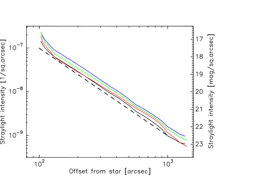
Figure 7: Star image (aureole) profiles as measured over the offset range of 100″  -1400″ . The intensity scale on the left-hand y-axis is in units of the star’s flux per arcsec² . The righthand scale is in units of mag arcsec^-2 when the star is of magnitude zero. Selected wavelength slots are displayed as black (360–380 nm), blue (400–420 nm), green (480–500 nm) and red (560–580 nm) lines. For reference the star profile of King (1971) is shown as dashed line.

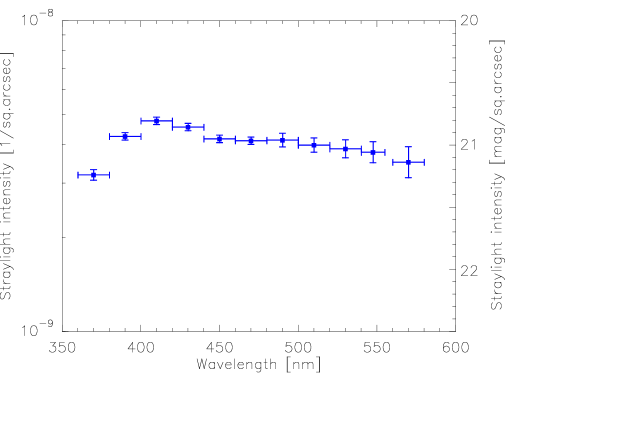
Figure 8: Stray light intensity at 600″  offset as function of wavelength, calculated from linear least-squares fits to observed curves between 120″ – 1400″. Left- and right-hand y-axis scales are as in Fig. B1. Horizontal bars indicate the wavelength ranges and the intensity errors are from the fits.

Appendix C Optical intermediate band and infrared 200 $\mn@boldsymbol{\mu}{\bf m}$ surface photometry of L 1642

An intermediate band surface photometry of selected positions in the area of L 1642 has been carried out in five filters, centred at 360 nm $(u)$, 385 nm, 415 nm, 470 nm $(b)$ and 555 nm $(y)$, using the ESO 1-m and 50-cm telescopes at La Silla (Mattila & Schnur 1990; Mattila, Väisänen, & von Appen-Schnur 1996; see also Laureijs, Mattila, & Schnur 1987). The 50-cm telescope monitored the airglow variations. The observations were made differentially, relative to a standard position (Pos8, see Table 2) in the centre of the cloud. Subsequently, the zero level was set by fitting in Dec, RA coordinates a plane through the darkest positions well outside the bright cloud area.

The ISOPHOT instrument (Lemke et al., 1996) aboard the $ISO$ satellite (Kessler et al., 1996) has been used to map an area of $\sim$1.2 $\sq\degr$ around L 1642 at 200 $\mu$m (Lehtinen et al., 2004, 2007). In addition, the positions shown in Fig. 3 as circles (photometry only) and squares (photometry and spectrophotometry) were observed also in the absolute photometry mode with ISOPHOT at 200 $\mu$m.

C.1 Relationship between optical and 200 $\mn@boldsymbol{\mu}{\bf m}$ surface brightness

The relationship between optical and 200 $\mu$m surface brightness is used in Appendix B to estimate the $B$ and $V$ band surface brightness distribution in L 1642. In Fig. C1 the optical surface brightness values, $I_{\lambda}^{\rm opt}$, at 415, 470 and 555 nm are shown as function of the 200 $\mu$m surface brightness, $I_{200}$.

At small optical depths with $A_{\lambda}\la 1$ mag, corresponding to $I_{200}\la 20$ MJy, the relationship is closely linear. At intermediate opacity positions, with $A_{\lambda}\sim$1–2 mag, the scattered light has its maximum value. For still larger optical depths the scattered light intensity decreases because of extinction and multiple scattering and absorption losses.

We have derived a relationship of the following form between the optical and the 200 $\mu$m surface brightnesses:

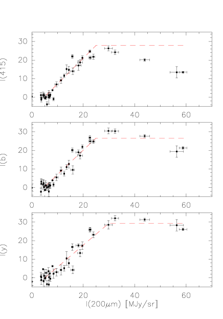
Figure 9: Optical surface brightness in the intermediate band filters at 415 nm, 470 nm $(b)$ and 555 nm $(y)$ vs $I_{\rm 200}$ in the L 1642 area. The unit for optical surface brightness is $10^{-9}$ erg cm^-2s^-1sr^-1Å^-1 .

$$I_{\lambda}^{\rm opt}=k\cdot I_{200}+b$$ (15)

when $I_{200}\leq I_{200}^{0}$, and

$$I_{\lambda}^{\rm opt}=const.=k\cdot I^{0}_{200}+b$$ (16)

when $I_{200}>I^{0}_{200}$. Here $I_{200}^{0}$ designates the value at which the optical surface brightness saturates and the linear relationship is no longer valid. Because the high opacity area with $I_{200}>I_{200}^{0}$ covers only a small central part of the cloud the approximation with $I_{\lambda}^{\rm opt}$ = const was considered to be sufficiently good for the present purpose. The optical surface brightness values are background-subtracted ones, the background being defined by the OFF-source positions with the lowest $I_{200}$ values. The parameter values for the three observed intermediate bands and the thereof estimated values for the $B$ and $V$ bands are given in Table C1.

Table 6: Parameters of the relationship between the optical and the 200 $\mu$m surface brightness in the L 1642 area. The parameters $k$ , $b$ and $I_{200}^{0}$ are defined by equations (C1) and (C2). The units are $k$: $10^{-9}$ erg cm^-2s^-1sr^-1Å^-1 /MJy sr^-1; $b$: $10^{-9}$ erg cm^-2s^-1sr^-1Å^-1  and $I^{0}_{200}$: MJy sr^-1.

$\lambda$	415 nm	470 nm	550 nm	$B$	$V$
$k$	$1.38$	$1.31$	$1.18$	1.35	1.18
	$\pm 0.09$	$\pm 0.07$	$\pm 0.07$	$\pm 0.09$	$\pm 0.07$
$b$	$-6.6$	$-6.1$	$-6.0$	-6.35	-6.0
	$\pm 0.9$	$\pm 0.9$	$\pm 1.0$	$\pm 0.9$	$\pm 1.0$
$I^{0}_{200}$	25	25	30	25	30

C.2 Relationship between optical extinction and 200 $\mn@boldsymbol{\mu}{\bf m}$ surface brightness

For low to moderate extinctions the 200 $\mu$m intensity is linearly correlated with the optical extinction, $A_{\rm V}$, (see e.g. Lehtinen et al. 2007). We first used the nicer method (Lombardi & Alves, 2001) to derive extinctions from the 2MASS $JHK$ colour excesses of stars in $\O$$6\arcmin$ areas corresponding to our spectrophotometry positions in Table 1. However, because of the relatively low surface density of 2MASS stars at the high galactic latitude of L 1642 these extinction values had large statistical errors of ca. $\pm 0.2-0.3$ mag. The high precision achieved for $I_{200}$ values (ca. $\pm 0.5$ MJy sr^-1) allows a better accuracy to be reached for $A_{\rm V}$, especially at low extinctions. Therefore, visual extinctions for our low-to-moderate extinction positions, $A_{V}\la 1$mag, were determined in the following way using ISOPHOT 200 $\mu$m absolute photometry observations.

A fit to $I_{200}$ vs $A_{\rm V}$ at $I_{200}<$30 MJy sr^-1 gave the slope of $19.0\pm 2.5$ MJy sr^-1mag^-1. The zero point of $I_{200}$ was corrected for a Zodiacal Emission (ZE) of $0.8\pm 0.2$ MJy sr^-1 and a CIB of $1.1\pm 0.3$ MJy sr^-1 (Hauser et al., 1998). The ZE at time of our 200 $\mu$m observations (1998-03-19/20, longitude difference $\lambda$(L 1642)-$\lambda_{\sun}=63\aas@@fstack{\circ}7)$ was estimated using a 270 K blackbody fit to the ZE intensities at 100, 140 and 240 $\mu$m. They were interpolated from the weekly DIRBE Sky and Zodi Atlas (DSZA) maps based on the Kelsall et al. (1998) interplanetary dust distribution model. The extinction values were then calculated from
$A_{\rm V}=(I_{200}-1.9$ MJy sr^-1)/19 MJy sr^-1mag^-1
and are given for our spectrophotometric positions in Table 1. We estimate their errors to be ca. $\pm 0.05$ mag.

Appendix D The spectra in numerical form

The resulting spectra for Positions 8, 9, 42, and the mean of 9 and 42 as discussed in Section 8 and displayed in Fig. 6 are available in the form of machine readable ASCII.txt files as an attachment to the electronic version of this Paper. The files are named Pos8.txt, Pos9.txt, Pos42.txt, and Pos9_42.txt. Each file has two columns: the wavelength ranging from 3649 to 5955 Å  and the intensity in units of $10^{-9}$ erg cm^-2s^-1sr^-1Å^-1 .

References

- Aharonian et al. (2006) Aharonian, F., et al., 2006, Nature, 440, 1018
- Ackermann et. al. (2012) Ackermann, M.,et al., 2012, Science, 338, 1190
- Appenzeller et al. (1998) Appenzeller I., et al., 1998, Msngr, 94, 1
- Ashburn (1954) Ashburn E. V., 1954, JATP 5, 83 (reprinted in JGR, 59, 67)
- Beckers (1995) Beckers J. M., 1995, in International Symposium on the Scientific and Engineering Frontiers for 8 - 10 m Telescopes, p. 303
- Bernstein (2007) Bernstein R. A., 2007, ApJ, 666, 663
- Bernstein et al. (2002a) Bernstein, R.A., Freedman, W. L., & Madore, B. F. 2002 ApJ, 571, 56
- Bernstein et al. (2002b) Bernstein, R.A. et al. 2002 ApJ, 571, 107
- Bernstein et al. (2005) Bernstein, R.A., Freedman, W. L., & Madore, B. F. 2005 ApJ, 632, 713
- Biteau & Williams (2015) Biteau J., Williams D. A., 2015, ApJ, 812, 60
- Bruzual A. (1983) Bruzual A. G., 1983, ApJ, 273, 105
- Chandrasekhar (1950) Chandrasekhar, S., 1950, Radiative Transfer. Oxford, Clarendon Press
- Domínguez et al. (2013) Domínguez A., Finke J. D., Prada F., Primack J. R., Kitaura F. S., Siana B., Paneque D., 2013, ApJ, 770, 77
- Dressler & Shectman (1987) Dressler A., Shectman S. A., 1987, AJ, 94, 899
- Hamilton (1985) Hamilton D., 1985, ApJ, 297, 371
- Hauser et al. (1998) Hauser M. G., et al., 1998, ApJ, 508, 25
- Hearty et al. (2000) Hearty T., Fernández M., Alcalá J. M., Covino E., Neuhäuser R., 2000, A&A, 357, 681
- H.E.S.S. Collaboration (2013) H.E.S.S. Collaboration 2013, A&A 550, A4
- Hg et al. (2000) Hg, E., et al., 2000, A&A, 355, L27
- Juvela et al. (2009) Juvela M., Mattila K., Lemke D., Klaas U., Leinert C., Kiss C., 2009, A&A, 500, 763
- Kelsall et al. (1998) Kelsall, T. et al. 1998 ApJ, 508, 44
- Kessler et al. (1996) Kessler M. F., et al., 1996, A&A, 315, L27
- King (1971) King I. R., 1971, PASP, 83, 199
- Kurucz et al. (1984) Kurucz R. L., Furenlid I., Brault J., Testerman L., 1984, Solar Flux Atlas from 296 to 1300 nm
- Laureijs, Mattila, & Schnur (1987) Laureijs R. J., Mattila K., Schnur G., 1987, A&A, 184, 269
- Lehtinen et al. (2004) Lehtinen K., Russeil D., Juvela M., Mattila K., Lemke D., 2004, A&A, 423, 975
- Lehtinen et al. (2007) Lehtinen K., Juvela M., Mattila K., Lemke D., Russeil D., 2007, A&A, 466, 969
- Lehtinen & Mattila (2013) Lehtinen K., Mattila K., 2013, A&A, 549, A91 Lehtinen K., Juvela M., Mattila K., Lemke D., Russeil D., 2007, A&A, 466, 969
- Leinert et al. (1998) Leinert, C. et al. 1998, A&AS 127, 1
- Lemke et al. (1996) Lemke D., et al., 1996, A&A, 315, L64
- Lombardi & Alves (2001) Lombardi M., Alves J., 2001, A&A, 377, 1023
- Longair (1995) Longair M. S., 1995, in The Deep Universe, ed. B. Binggeli & R. Buser, (Saas-Fee Advanced Course 23; Berlin: Springer), 317
- Matsuoka et al. (2011) Matsuoka, Y., Ienaka, N., Kawara, K., Oyabu S., 2011, ApJ, 736, 119
- Mattila (1970) Mattila, K. 1970, A&A, 9, 53
- Mattila (1976) Mattila, K. 1976, A&A, 47, 77
- Mattila (1980a) Mattila K., 1980a, A&A, 82, 373
- Mattila (1980b) Mattila K., 1980b, A&AS, 39, 53
- Mattila & Schnur (1990) Mattila, K. & Schnur,G. 1990, IAU Symposium No. 139, 257
- Mattila, Väisänen, & von Appen-Schnur (1996) Mattila K., Väisänen P., von Appen-Schnur G. F. O., 1996, A&AS, 119, 153
- Mattila (2003) Mattila, K. 2003, ApJ, 591, 119
- Mattila et al. (2012) Mattila K., Lehtinen K., Väisänen P., von Appen-Schnur G., Leinert C., 2012, IAUS, 284, 429
- Mattila et al. (2017b) Mattila K., Väisänen P., Lehtinen K., von Appen-Schnur G., Leinert C., 2017b, MNRAS, xx, yy (Paper II)
- Michard (2002) Michard R., 2002, A&A, 384, 763
- Partridge & Peebles (1967) Partridge, B., Peebles, P.J.E. 1967, ApJ, 148, 377
- Patat (2003) Patat F., 2003, A&A, 400, 1183
- Patat et al. (2011) Patat F., et al., 2011, A&A, 527, A91
- Puget et al. (1996) Puget J.-L., Abergel A., Bernard J.-P., Boulanger F., Burton W. B., Desert F.-X., Hartmann D., 1996, A&A, 308, L5
- Tody (1993) Tody D., 1993, ASPC, 52, 173
- Toller (1983) Toller G. N., 1983, ApJ, 266, L79
- Tüg (1977) Tüg H., 1977, Msngr, 11, 7
- Väisänen (1996) Väisänen,P. 1996, A&A 315, 21
- Windhorst et al. (2011) Windhorst R. A., et al., 2011, ApJS, 193, 27
- Zacharias et al. (2004) Zacharias N., Monet D. G., Levine S. E., Urban S. E., Gaume R., Wycoff G. L., 2004, AAS, 36, 1418
- Zacharias et al. (2005) Zacharias N., Monet D. G., Levine S. E., Urban S. E., Gaume R., Wycoff G. L., 2005, yCat, 1297, 0
- Zemcov et al. (2014) Zemcov M., et al., 2014, Sci, 346, 732
- Zemcov et al. (2017) Zemcov M., Immel P., Nguyen C., Cooray A., Lisse C. M., Poppe A. R., 2017, Nature Communications, 8, A15003
Acknowledgements
We thank the ESO staff at Paranal and in Garching for their excellent service
and an anonymous referee for suggesting several improvements to the paper.
This research has made use of the USNOFS Image and Catalogue archive
operated by the United States Naval Observatory, Flagstaff Station
(http://www.nofs.navy.mil/data/fchpix/).
The Digitized Sky Surveys were produced at the Space Telescope Science Institute
under U.S. Government grant NAG W-2166. The images of these surveys are based on
photographic data obtained using the Oschin Schmidt Telescope on Palomar Mountain
and the UK Schmidt Telescope. The plates were processed into the present compressed
digital form with the permission of these institutions. KM and KL acknowledge the
support from the Research Council for Natural Sciences and Engineering (Finland) and PV
acknowledges the support from the National Research Foundation of South Africa.