Duality between the deconfined quantum-critical point and the
bosonic topological transition

Abstract

Recently significant progress has been made in $(2+1)$-dimensional conformal field theories without supersymmetry. In particular, it was realized that different Lagrangians may be related by hidden dualities, i.e., seemingly different field theories may actually be identical in the infrared limit. Among all the proposed dualities, one has attracted particular interest in the field of strongly-correlated quantum-matter systems: the one relating the easy-plane noncompact CP¹ model (NCCP¹) and noncompact quantum electrodynamics (QED) with two flavors ($N=2$) of massless two-component Dirac fermions. The easy-plane NCCP¹ model is the field theory of the putative deconfined quantum-critical point separating a planar (XY) antiferromagnet and a dimerized (valence-bond solid) ground state, while $N=2$ noncompact QED is the theory for the transition between a bosonic symmetry-protected topological phase and a trivial Mott insulator. In this work we present strong numerical support for the proposed duality. We realize the $N=2$ noncompact QED at a critical point of an interacting fermion model on the bilayer honeycomb lattice and study it using determinant quantum Monte Carlo (QMC) simulations. Using stochastic series expansion QMC, we study a planar version of the $S=1/2$ $J$-$Q$ spin Hamiltonian (a quantum XY-model with additional multi-spin couplings) and show that it hosts a continuous transition between the XY magnet and the valence-bond solid. The duality between the two systems, following from a mapping of their phase diagrams extending from their respective critical points, is supported by the good agreement between the critical exponents according to the proposed duality relationships.

I Introduction

A duality in physics is an equivalence of different mathematical descriptions of a system or a state of matter, established through a mapping by change of variables. The simplest example is the particle-wave duality in quantum mechanics, where the duality transformation is a change of basis by Fourier transformation, and the chosen basis dictates the variables used to describe the system. In classical statistical mechanics, the most famous duality is the Kramers-Wannier duality of the two-dimensional (2D) Ising model Kramers and Wannier (1941). Here the low- and high-temperature expansions of the partition function can be related to each other by identifying a one-to-one correspondence between the terms in the two different series, thus establishing an exact mapping between the ordered and disordered phases and the corresponding collective variables. In this case the critical point is also a self-duality point. In the 3D Ising model, one can instead find a different model whose high-temperature expansion stands in a direct one-to-one correspondence with the low-temperature expansion of the the Ising gauge model Kogut (1979); Savit (1980). Many other examples of dualities have been established, e.g., the well-known equivalence between the 3D O(2) Wilson-Fisher fixed point and the 3D Higgs transition with a noncompact U(1) gauge field Peskin (1978); Dasgupta and Halperin (1981); Fisher and Lee (1989) .

In analogy with the Ising examples mentioned above, it is some times possible to transform a quantum field theory at strong coupling into an equivalent dual theory at weak coupling. The untractable original problem can then be solved by means of perturbative methods applied to the dual theory. Such strong-weak duality (and the more general “S-duality” form) was established in certain supersymmetric Yang-Mills theories Montonen and Olive (1977); Seiberg (1995); Seiberg and Witten (1994a, b) and Abelian gauge theory without super-symmetry Cardy and Rabinovici (1982); Cardy (1982); Witten (1995). In 1D quantum systems (i.e., in $1+1$ space-time dimensions) a well known fermion-boson duality is achieved by bosonization of an interacting fermion system through a non-local transformation Coleman (1975); Mandelstam (1975); Luther and Peschel (1974); Witten (1984); Giamarchi (2004). Usually, in the bosonized formalism interactions can be more easily treated than in the original fermion model.

In cases where no formal mapping is known, two Lagrangians that look different in the ultraviolet may still flow (under the renormalization group) to the same theory in the infrared, i.e., these seemingly different field theories actually represent exactly the same low-energy physics. Such a duality goes a step beyond the more familiar concept of universality, by which systems (models or real materials) with the same dimensionality and global symmetries exhibit identical scaling properties at their classical or quantum critical points. Such systems share the same effective critical low-energy field-theory description. For example, the critical points of the Bose-Hubbard model and the quantum rotor model are in the same universality class. A duality transformation usually changes the description of the system into a form based on nonlocal objects or defects of the original description. On a practical level, the existence of a dual field theory means that there is a non-trivial choice of which description to use, and one of them (and not necessarily the originally most obvious one) may pose a more tractable setup for calculations.

Even if no strong-weak transformation exists (or is known), a difficult or non-tractable strong-coupling problem can some times be shown to be dual to a different strong-coupling problem that is tractable with some specific computational technique. In particular, the dual problem may be more easily solvable using powerful numerical (lattice) methods. In this paper we will explore such a recently proposed duality between two different $(2+1)$D Lagrangians that respectively involve fermionic and bosonic matter fields coupled with a gauge field Potter et al. (2016); Wang et al. (2017). Both theories are of great current interest in the context of strongly correlated electrons in two dimensions. Our aim here is to identify a duality between the systems by establishing corresponding lattice models realizing the two low-energy theories.

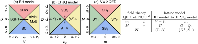
We follow the recent proposal that $(2+1)$D quantum electrodynamics (QED) with noncompact gauge field and two flavors of Dirac fermions is dual to the critical point of the easy-plane NCCP¹ model (the bosonic QED with two flavors of complex bosons) Potter et al. (2016); Wang et al. (2017). On the lattice, we realize the former with an interacting fermion model with spin-orbit coupling on the bilayer honeycomb lattice (BH), which hosts a quantum phase transition between a (bosonic) symmetry-protected topological state and a trivial Mott insulator Slagle et al. (2015); He et al. (2016a); Wu et al. (2016). It was proposed that this transition is described by $N=2$ noncompact QED Grover and Vishwanath (2013a); Lu and Lee (2014). To realize the low-energy physics of the NCCP¹ theory, in this paper we introduce a planar variant of the spin $S=1/2$ $J$-$Q$ Hamiltonian (a Heisenberg model with additional multi-spin couplings Sandvik (2007)), dubbed the easy-plane $J$-$Q$ (EPJQ) model, and show that it hosts a deconfined quantum-critical point Senthil et al. (2004a, b); Senthil and Fisher (2006) separating antiferromagnetic (AFM) and dimerized (valence-bond-solid, VBS) ground states (similar to the case of the $J$-$Q$ model with full spin SU(2) symmetry Shao et al. (2016), but with different universality due to the lowered symmetry). Our numerical (quantum Monte Carlo, QMC) results establishes the critical-point universality and duality between the phase diagrams of the two models. With the EPJQ model being much easier to study on large scales with QMC simulations than the fermionic model, the duality that we establish here allows for detailed studies of the topological transition of the latter, through the analogue of the deconfined quantum-critical point. The phase diagrams and dualities studied are summarized in Fig. 1.

The rest of the paper is organized as follows: In Sec. II we present the details of the two field theories and their putative duality, and in Sec. III we define the lattice models and the proposed mappings relating their phase diagrams to each other. In Sec. IV and Sec. V we present the numerical results for the EPJQ and BH models, respectively. We conclude with a brief summary and discussion of the results in Sec. VI. In Appendix A we present further technical details on the analysis of the critical exponents, and in Appendix B we compare results for different variants of the EPJQ model (with different degrees of spin-anisotropy).

II Continuum field theories

The bosonic particle-vortex duality mentioned in the introduction was recently generalized to a model with fermionic matter Son (2015); Wang and Senthil (2016a, 2015, b); Metlitski and Vishwanath (2016); Seiberg et al. (2016); Kachru et al. (2017, 2016); Mross et al. (2016), in the form of a $(2+1)$D QED Lagrangian with a single flavor of a two component Dirac fermion and noncompact gauge field, i.e., $N=1$ QED. This theory is dual to that of a noninteracting Dirac fermion in the infrared limit . Based on this $N=1$ duality, Ref. Xu and You (2015) showed that $(2+1)$D QED with noncompact gauge field and $N=2$ flavors of Dirac fermions is self-dual. This is also a fermionic version of the self-duality of the easy-plane NCCP¹ model (which can be regarded as $N=2$ bosonic QED) Motrunich and Vishwanath (2004); Senthil et al. (2004a, b). The self-duality of the $N=2$ QED Lagrangian was also verified with different derivations Mross et al. (2016); Karch and Tong (2016); Hsin and Seiberg (2016). Unlike the case of $N=1$, there is no equivalent noninteracting description of $(2+1)$D QED with $N=2$, however. Because of its self-duality, $N=2$ QED hosts an (emergent) O($4$) symmetry in the infrared, which factorizes into the two independent SU($2$) flavor symmetries on the two sides of the self-dual point.

More recently, based on the previous fermion-boson duality Seiberg et al. (2016), it was argued that $N=2$ QED is also dual to the easy-plane NCCP¹ model at the critical point Potter et al. (2016); Wang et al. (2017). These two field theories can be written as

$$\mathcal{L}_{\text{QED}}=\bar{\psi}\gamma\cdot(\partial-\mathrm{i}a)\psi+m\bar{\psi}\psi+M\bar{\psi}\sigma^{3}\psi,$$ (1a)

$$\mathcal{L}_{\text{CP${}^{1}$}}=|(\partial-\mathrm{i}b)z|^{2}+g|z|^{4}+rz^{\dagger}z+hz^{\dagger}\sigma^{3}z,$$ (1b)

where $\psi$ and $z$ are two-component Dirac fermion and complex boson fields coupled to non-compact U(1) gauge fields, $a$ and $b$, respectively. The duality maps the variables $(m,M)$ to $(h,r)$. Moreover, both theories in Eq. (1) are individually self-dual. The putative duality between the two theories implies that the easy-plane NCCP¹ model should also have an emergent O($4$) symmetry at its critical point, which is not immediately obvious in Eq. (1b). The corresponding O($4$) order parameter is

$$\boldsymbol{N}=\left(z^{\dagger}\sigma^{x}z,z^{\dagger}\sigma^{y}z,\mathrm{Re}[\mathcal{M}_{b}],\mathrm{Im}[\mathcal{M}_{b}]\right),$$ (2)

where $\mathcal{M}_{b}$ is the monopole operator (gauge flux annihilation operator) of the gauge field $b$.

Figure 1: Schematic phase diagrams of (a) the bilayer honeycomb (BH) model, (b) the easy-plane $J$-$Q_{3}$ (EPJQ) model, and (c) the $N=2$ QED theory. In (a), the BH model contains two symmetry-breaking phases: the spin-density-wave (SDW) and superconducting (SC) phases, and two symmetric phases: the bosonic symmetry-protected topological (BSPT) and the trivial Mott-insulating phases. In (b), the EPJQ model also contains two symmetry-breaking phases: the Néel antiferromagnetic (AFM) phase and the valence-bond solid (VBS) phase, and two spin-polarized phases induced by an external staggered field. In (c), as was shown in Ref. Grover and Vishwanath (2013b); Lu and Lee (2014); Wang et al. (2017), when tuning the two masses $m$ and $M$, the $N=2$ QED theory also has two symmetry-breaking (SB) phases and two symmetric (SY) phases, one of which is the BSPT state. In all models, the four phases merge at the deconfined quantum critical point. Phases of the same color can be mapped to each other among the models, following the duality relations proposed in the table on the right. The double arrows in (a) and (b) indicate the quantum phase transitions investigated numerically in this paper.

The proposed duality between the two theories in Eq. (1) leads to very strong predictions for relationships between their properties. For example, the scaling dimension of $m$ in $N=2$ QED should be precisely the same as the scaling dimension of $h$ in the easy-plane NCCP¹ at its critical point $r=0$, while the scaling dimension of $M$ should be the same as that of $r$. Also, as a consequence of these dualities, i.e., the emergent O($4$) symmetry of the two theories, the four components of $\boldsymbol{N}$ should all have the same scaling dimension at the critical point.

Although the duality can be observed and “derived” based on various arguments, it has not been rigorously proven yet. Both Eq. (1a) and Eq. (1b) are strongly interacting conformal field theories, and there is no obvious analytical method that can provide rigorous results for either case. However, both theories can presumably be realized using lattice models, which can be simulated using numerical methods. The goal of this work is to compare the quantitative properties of such lattice models and look for evidence of the proposed duality. As we will show in the later sections, within small error bars of the critical exponents obtained using QMC simulations, our results confirm several predictions of the duality.

Because the duality of the two theories in Eq. (1) was derived based on the assumption of the basic fermion-boson duality Chen et al. (1993); Seiberg et al. (2016), a proof of the former duality indirectly also proves the latter. In principle this result can lead to a number of further dualities between different fermionic and bosonic Lagrangians. Thus, the impact of our work is not limited to the proof of the duality between Eq. (1a) and Eq. (1b), but also provides justification for many other cases.

III Lattice models

The easy-plane NCCP¹ model is the field theory that presumably describes the deconfined quantum-critical point between an in-plane (XY) antiferromagnet (AFM) and a valence-bond solid (VBS) Motrunich and Vishwanath (2004); Senthil et al. (2004a, b). This transition in the case of full SU(2) symmetry of the Hamiltonian has been realized by the $J$-$Q$ and related models, and these have been extensively simulated numerically using unbiased QMC techniques Sandvik et al. (2002); Sandvik (2007); Lou et al. (2009); Sen and Sandvik (2010); Sandvik (2010); Nahum et al. (2011); Harada et al. (2013); Pujari et al. (2013, 2015); Nahum et al. (2015a, b); Shao et al. (2016). Although there are studies that indicate that some version of the $J$-$Q$ model with an inplane spin symmetry and other U(1) symmetric models should lead to a first order transition Kuklov et al. (2008); Geraedts and Motrunich (2012); D’Emidio and Kaul (2016, 2017), in this work we demonstrate that a different model, the EPJQ model, instead leads to a continuous transition in some regions of its parameter space. The $r$ and $h$ terms in Eq. (1) correspond to the distance from the critical point, $Q-Q_{c}$, and the staggered magnetic field $h_{z}(-)^{i}S^{z}_{i}$, respectively, in the lattice model. The components of the O(4) vector in Eq. (2) correspond to the two-component easy-plane Néel and two-component VBS (dimer) order parameters of the EPJQ model.

The $N=2$ QED action has been simulated directly using a lattice QED model Karthik and Narayanan (2016), and the scaling dimension of $M$ was computed in this way. Also, $N=2$ QED with a noncompact U(1) gauge field is the effective theory that describes the transition between the bosonic symmetry protected topological (BSPT) state and a trivial Mott state in $2D$ Grover and Vishwanath (2013a); Lu and Lee (2014). This transition was also realized in an interacting fermion model on a bilayer honeycomb (BH) lattice introduced in Refs. Slagle et al. (2015); He et al. (2016a) and simulated Slagle et al. (2015); He et al. (2016a, b); Wu et al. (2016) with a determinantal QMC method (DQMC) Meng et al. (2010, 2014). The $m$ and $M$ terms in Eq. (1) correspond to two different interactions in the lattice model, namely, the interlayer pair-hopping $V-V_{c}$, measured with respect to its critical value, and the Hubbard-like on-site interaction $U$; the Hamiltonian will be specified in detail below. The lattice model of Ref. He et al. (2016a) has an exact SO(4) symmetry that precisely corresponds to the proposed emergent symmetry of the $N=2$ QED. It should further be noted that the fermions in the BH model do not directly correspond to the Dirac fermions of the $N=2$ QED action, because the former are not coupled to any dynamical gauge field. The relation between the two systems instead arises from the correspondence of the gauge invariant fields of $N=2$ QED to the low-energy bosonic excitations of the BH model.

Using the BH model and the EPJQ model, the duality between the $N=2$ QED and the NCCP¹ field theories can be realized on the lattice. The O(4) vector $\boldsymbol{N}$ can also be conveniently defined in both lattice models, with explicit forms that will be explained below. Thus, the two systems can be investigated and compared via unbiased large-scale QMC simulations—the pursuit and achievement of this work.

In the following, we will first define the microscopic lattice models in detail. In the subsequent sections IV and V we present comparative numerical studies of the models and demonstrate strong support for the duality relations listed in the table in Fig. 1.

III.1 Bilayer honeycomb model

The BH model is a fermionic model defined on a honeycomb lattice Slagle et al. (2015); He et al. (2016a, b); Wu et al. (2016). On each site, we define four flavors of fermions (two layers $\times$ two spins);

$$c_{i}=(c_{i1\uparrow},c_{i1\downarrow},c_{i2\uparrow},c_{i2\downarrow})^{\intercal}.$$ (3)

The Hamiltonian is

$$H_{\text{BH}}=H_{\text{band}}+H_{\text{int}},$$ (4)

where the band and interaction terms are given by

$$H_{\text{band}} =-t\sum_{\langle ij\rangle}c_{i}^{\dagger}c_{j}+\lambda\sum_{\langle\!\langle ij\rangle\!\rangle}\mathrm{i}\nu_{ij}(c_{i}^{\dagger}\sigma^{3}c_{j}+\text{h.c.}),$$ (5a)

$$H_{\text{int}} =V\sum_{i}(c_{i1\uparrow}^{\dagger}c_{i2\uparrow}c_{i1\downarrow}^{\dagger}c_{i2\downarrow}+\text{h.c.}),$$ (5b)

where $\langle ij\rangle$ and $\langle\!\langle ij\rangle\!\rangle$ denote nearest-neighbor intra- and inter-layer site pairs, respectively. The band Hamiltonian $H_{\text{band}}$ is just two copies of the Kane-Mele model Kane and Mele (2005), which drives the fermion into a quantum spin Hall state with spin Hall conductance $\sigma_{\text{sH}}=\pm 2$ (depending on the sign of the spin-orbit coupling $\lambda$). Including a weak interaction $V$, the bilayer quantum spin Hall state automatically becomes a BSPT state He et al. (2016a); Wu et al. (2016); You et al. (2016), where only the bosonic O(4) vector $\boldsymbol{N}$ remains gapless (and protected) at the edge, while the fermionic excitations are gapped out (as will be discussed in more detail below). However, a strong interlayer pair-hopping interaction $V$ eventually favors a direct product state of anti-bonding Cooper pairs. In the strong interaction limit ($V\to\infty$), the ground state of the BH model reads

$$|\text{GS}\rangle=\prod_{i}(c_{i1\uparrow}^{\dagger}c_{i1\downarrow}^{\dagger}-c_{i2\uparrow}^{\dagger}c_{i2\downarrow}^{\dagger})|0_{c}\rangle,$$ (6)

with $|0_{c}\rangle$ being the fermion vacuum state. This state has no quantum spin Hall conductance, i.e., $\sigma_{\text{sH}}=0$, and, more importantly, it is a direct product of local wave functions, hence dubbed trivial Mott insulator state. It was found numerically that there is a direct continuous transition between the BSPT and the trivial Mott phases at $V_{c}/t=2.82(1)$ He et al. (2016a, b), where the single-particle excitation gap does not close but the excitation gap associated with the bosonic O(4) vector closes and the quantized spin Hall conductance changes from $\pm 2$ to $0$.

The low-energy bosonic fluctuations around the critical point form an O(4) vector, with $\boldsymbol{N}=(\mathrm{Re}\Sigma,\mathrm{Im}\Sigma,\mathrm{Re}\Delta,\mathrm{Im}\Delta)$ and the components are

$$\Sigma_{i} =(-1)^{i}(c_{i1\uparrow}^{\dagger}c_{i2\downarrow}+c_{i2\uparrow}^{\dagger}c_{i1\downarrow}),$$ (7a)

$$\Delta_{i} =(c_{i1\downarrow}c_{i1\uparrow}-c_{i2\downarrow}c_{i2\uparrow}),$$ (7b)

where $\Sigma$ carries spin and $\Delta$ carries charge. The BH model Eq. (4) respects the global $\text{SO}(4)$ symmetry of the vector $\boldsymbol{N}$. If the symmetry is lowered to $\text{U}(1)_{\text{spin}}\times\text{U}(1)_{\text{charge}}$, then, based on the analysis of $N=2$ QED, in principle the mass term $M\bar{\psi}\sigma^{3}\psi$ is allowed; hence the BSPT-Mott transition is unstable towards spontaneous symmetry-breaking of the remaining symmetries. The symmetry of the mass term $M\bar{\psi}\sigma^{3}\psi$ is identical to the following Hubbard-like interaction (both forming a $(1,1)$ representation of the SO(4)):

$$\frac{U}{2}\sum_{i}(\Delta_{i}^{\dagger}\Delta_{i}+\Delta_{i}\Delta_{i}^{\dagger}-\Sigma_{i}^{\dagger}\Sigma_{i}-\Sigma_{i}\Sigma_{i}^{\dagger})=U\sum_{i}\rho_{i\uparrow}\rho_{i\downarrow}.$$ (8)

Here $\rho_{i\sigma}$ is the density operator (for $\sigma=\uparrow,\downarrow$ spins),

$$\rho_{i\sigma}=(c_{i1\sigma}^{\dagger}c_{i1\sigma}+c_{i2\sigma}^{\dagger}c_{i2\sigma}-1),$$ (9)

which counts the number of $\sigma$-spin fermions in both layers on site $i$ with respect to half-filling. The repulsive $U>0$ (or attractive $U<0$) interaction drives spin $\langle\Sigma\rangle\neq 0$ (or charge $\langle\Delta\rangle\neq 0$) condensation, leading to a spin-density wave (SDW) Wu et al. (2016) (or superconducting) phase that breaks the $\text{U}(1)_{\text{spin}}$ [or $\text{U}(1)_{\text{charge}}$] symmetry spontaneously. This process is illustrated in the schematic phase diagram Fig. 1(a).

III.2 Easy-plane JQ model

Our EPJQ model is a spin-$1/2$ system with anisotropic antiferromagnetic couplings which we here define on the simple square lattice of $L^{2}$ sites and periodic boundary conditions. It is a “cousin” model of the previously studied SU(2)${}_{\text{spin}}$ $J$-$Q_{3}$ model Lou et al. (2009); Sen and Sandvik (2010); Sandvik (2010)which in turn is an extension of the original $J$-$Q$, or $J$-$Q_{2}$, model Sandvik (2007). Starting from the spin-$1/2$ operator $\boldsymbol{S}_{i}$ on each site $i$, we define the singlet-projection operator on lattice link $ij$;

$$P_{ij}=\tfrac{1}{4}-\boldsymbol{S}_{i}\cdot\boldsymbol{S}_{j},$$ (10)

then the model Hamiltonian reads

$$H_{\text{JQ}}=-J\sum_{\langle ij\rangle}(P_{ij}-\Delta S_{i}^{z}S_{j}^{z})-Q\hskip-5.69054pt\sum_{\langle ijklmn\rangle}\hskip-5.69054ptP_{ij}P_{kl}P_{mn},$$ (11)

where the $\Delta S_{i}^{z}S_{j}^{z}$ term for $\Delta\in(0,1]$ introduces the easy-plane anisotropy that breaks the $\text{SU}(2)_{\text{spin}}$ symmetry down to $\text{U}(1)_{\text{spin}}$ explicitly. We have studied two cases: the maximally-planar case $\Delta=1$ and the less extreme case $\Delta=1/2$. In the latter case, we observe very good scaling behaviors indicating a continuous transition, with rapidly decaying (with the system size $L$) scaling corrections, while for $\Delta=1$ the behavior suggests a first-order transition. Thus, the model may harbor a tricritical point separating first-order and continuous transitions somewhere between $\Delta=1/2$ and $\Delta=1$. However, we will leave the possible tricritical point to future investigation. As far as the duality is concerned, in this section we discuss our results for $\Delta=1/2$, and in Appendix B we present results for $\Delta=1$.

We set $J+Q=1$ in the simulations and define the control parameter as the ratio

$$q=\frac{Q}{J+Q}.$$ (12)

For small $q$, the model essentially reduces to an XXZ model, which has an XYAFM ground state that breaks the $\text{U}(1)_{\text{spin}}$ symmetry spontaneously. When $q$ is large, the dimer interaction favors a VBS (columnar-dimerized) ground state, which breaks the lattice $C_{4}$ rotation symmetry as in the $\text{SU}(2)_{\text{spin}}$ $J$-$Q_{2}$ and $J$-$Q_{3}$ models Sandvik et al. (2002); Sandvik (2007); Lou et al. (2009); Sen and Sandvik (2010); Sandvik (2010); Shao et al. (2016), where previous QMC studies found a direct continuous AFM-VBS transition. Here we demonstrate that the continuous transition persists in EPJQ model, Eq. (11), with $\Delta=1/2$. The reason for choosing the $Q_{3}$ term (three-dimer interaction) instead of the simpler $Q_{2}$ interaction (two-dimer coupling) is that it produces a more robust VBS order when the ratio $q$ is large, thus leading to a smaller critical-point value [as in the SU(2) case Lou et al. (2009); Sen and Sandvik (2010)] with more clearly observable flows to the VBS state on that side of the transition.

The XYAFM order in the EPJQ model can be directly probed by the local spin components $S^{x}$ and $S^{y}$, and we will also study the critical fluctuations in the $S^{z}$ component. We will often not write out the staggered phase factor $(-1)^{x_{i}+y_{i}}$ corresponding to AFM order explicitly (here $x_{i}$ and $y_{i}$ refer to the integer-valued lattice coordinates of site $i$); in fact in the case of the XY-anisotropy in a model with bipartite interactions, the phase can also simply be transformed away with a sublattice rotation (and then the XYAFM phase maps directly onto hard-core bosons in the superfluid state). In our simulations the staggered phase is absent for the $S^{x}$ and $S^{y}$ components but present for the $S^{z}$ component. The AFM-VBS transition is unstable towards an axial Zeeman field, when $H_{\rm JQ}\to H_{\rm JQ}+H_{\rm Z}$ with

$$H_{\rm Z}=-h_{z}\sum_{i}(-1)^{x_{i}+y_{i}}S_{i}^{z},$$ (13)

which drives the system to the spin-polarized phase with $\langle S^{z}\rangle\neq 0$, as illustrated in the schematic phase diagram in Fig. 1(b). Here we consider only $h=0$.

To study the columnar VBS (dimer) order realized in the EPJQ model, we define

$$D^{x}_{i}=(-1)^{x_{i}}{\bf S}_{i}\cdot{\bf S}_{i+\hat{x}},$$ (14a)

$$D^{y}_{i}=(-1)^{y_{i}}{\bf S}_{i}\cdot{\bf S}_{i+\hat{y}},$$ (14b)

where ${i+\hat{x}}$ and ${i+\hat{y}}$ denote neighbors of site $i$ in the positive $x$ and $y$-direction, respectively. At the critical point, the proposed self-duality (through the putative duality with $N=2$ QED) implies that the $C_{4}$ rotation symmetry and the $\text{U}(1)_{\text{spin}}$ symmetry are enlarged into an emergent $\text{O}(4)$ symmetry, such that the components of the $\text{O}(4)$ vector (after some proper normalization)

$$\boldsymbol{N}=(D^{x},D^{y},S^{x},S^{y}),$$ (15)

should all have the same scaling dimension Wang et al. (2017).

III.3 Duality relations

Fig. 1 summarizes the intuitive duality relations among the BH, EPJQ, and QED models; this can also be observed from the similarity of their four-quadrant phase diagrams You and You (2016). To numerically prove the validity of these duality relations, in this work we investigate the following critical behaviors at the BSPT–Mott transition in the BH model:

$$\xi \sim|V-V_{c}|^{-\nu_{\text{BH}}},$$ (16a)

$$\langle\rho_{i\uparrow}\rho_{i\downarrow}\rho_{j\uparrow}\rho_{j\downarrow}\rangle \sim|\boldsymbol{r}_{ij}|^{-1-\eta^{\rho}_{\text{BH}}},$$ (16b)

$$\langle\Delta_{i}^{\dagger}\Delta_{j}\rangle \sim|\boldsymbol{r}_{ij}|^{-1-\eta^{\Delta}_{\text{BH}}};$$ (16c)

where $\boldsymbol{r}_{ij}$ is the lattice vector separating the sites $i,j$, $\xi$ is the correlation length of the critical O(4) bosonic modes of the system, and the density $\rho_{i\sigma}$ and pairing $\Delta_{i}$ operators have been defined in Sec. III.1. We also study the following expected critical scaling behavior at the AFM–VBS transition in the EPJQ model:

$$\xi \sim|Q-Q_{c}|^{-\nu^{xy}_{\text{JQ}}},$$ (17a)

$$\langle S_{i}^{z}S_{j}^{z}\rangle \sim|\boldsymbol{r}_{ij}|^{-1-\eta^{z}_{\text{JQ}}},$$ (17b)

$$\langle S_{i}^{+}S_{j}^{-}\rangle \sim|\boldsymbol{r}_{ij}|^{-1-\eta^{xy}_{\text{JQ}}}.$$ (17c)

where $\xi$ is the correlation length of the easy-plane spins.

If the duality in Eq. (1) is correct, and provided that $N=2$ QED is indeed the theory for the BSPT–Mott transition, then the exponents defined above must satisfy the following relationships Wang et al. (2017):

$$3-\frac{1}{\nu_{\text{BH}}}=\frac{1+\eta^{z}_{\text{JQ}}}{2},$$ (18a)

$$3-\frac{1}{\nu^{xy}_{\text{JQ}}}=\frac{1+\eta_{\text{QED}}}{2}=\frac{1+\eta^{\rho}_{\text{BH}}}{2},$$ (18b)

$$\eta^{\Delta}_{\text{BH}}=\eta^{xy}_{\text{JQ}}.$$ (18c)

Here $\eta_{\text{QED}}$ is the anomalous dimension of the fermion mass $\bar{\psi}\sigma^{3}\psi$, i.e., the $M$ mass term in our notation in Eq. (1a), which was numerically estimated in the recent lattice QED calculations in Ref. Karthik and Narayanan (2016).

IV Results for the EPJQ model

In this section we present our numerical results at the continuous AFM–VBS phase transition of the EPJQ model, obtained using large-scale SSE-QMC Sandvik (1999); Syljuåsen and Sandvik (2002) simulations. Here we discuss only the case $\Delta=1/2$ in the Hamiltonian Eq. (11); some results for $\Delta=1$ are presented in Appendix B. In the SSE simulations we scaled the inverse temperature as $\beta=2L$, corresponding to the dynamic exponent $z=1$ ($\beta\sim L^{z}$) and staying in the regime where the system is close to its ground state for each $L$. We consider $L$ up to $44$.

IV.1 Crossing-point analysis

The first step is to determine the order of the transition and the position of the critical point (if the transition is continuous). To this end, following the recent example in Ref. Shao et al. (2016) for the SU(2) $J$-$Q$ model, we first analyze crossing points of finite-size Binder cumulants, defined for the AFM order parameter as

$$U(q,L)=2-\frac{\langle M^{4}_{xy}\rangle}{\langle M^{2}_{xy}\rangle^{2}},$$ (19)

where $M^{2}_{xy}$ is the square of the easy-plane magnetization operator,

$$M^{2}_{xy}=\frac{1}{L^{4}}\sum_{i,j}(-1)^{i+j}S^{+}_{i}S^{-}_{j},$$ (20)

and $M^{4}_{xy}$ is its square. The “phenomenological renormalization” underlying the crossing-point analysis and our technical implementations of it are discussed in Appendix A. Here we show our numerical results and analyze them within the scaling relationships presented in the appendix.

Figure 2: Crossing-point analysis of the EPJQ model at $\Delta=1/2$. (a) $U(q,L)$ vs $q$ in the neighborhood of $q_{c}$ for several system sizes $L$. (b) The crossing points seen in (a) for system-size pairs $(L,2L)$, analyzed according to the expected finite-size scaling form, Eq. (21). The procedure including error analysis gives $q_{c}=0.6197(2)$ and $1/\nu^{xy}_{\text{JQ}}+\omega=4.0(2)$. (c) A similar analysis of $U^{*}_{c}(L)$, giving $\omega=2.3(1)$. (d) Finite-size estimates $\nu^{xy,*}_{\text{JQ}}$ of the correlation-length exponent defined in Eq. (23), using the slopes of the cumulants at the $(L,2L)$ crossing points. Analysis according to Eq. (24) gives $\nu^{xy}_{\text{JQ}}=0.48(2)$ for the exponent in the thermodynamic limit.

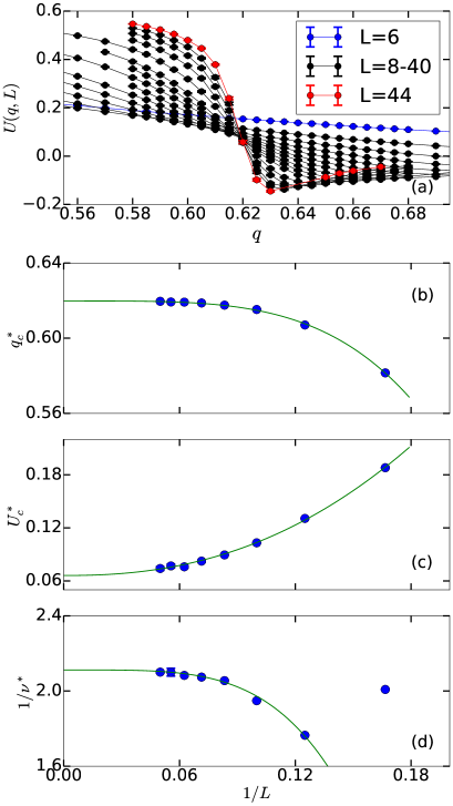
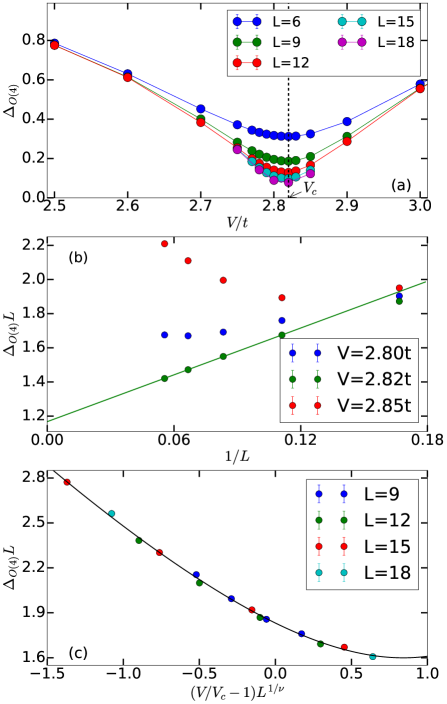
As shown in Fig. 2(a), curves of $U(q,L)$ graphed for different $L$ cross each other at points tending to a value $q_{c}$. In a finite-size system the deviation of $U(q,L)$ from the asymptotic crossing point depends on $L$ in a way that involves a scaling-correction exponent. For a finite-size pair $(L,2L)$, the crossing is at $[q^{*}_{c}(L),U^{*}_{c}(L)]$ and at a continuous transition one expects

$$q^{*}_{c}(L)=q_{c}+aL^{-(1/\nu^{xy}_{\text{JQ}}+\omega)},$$ (21)

where $\nu^{xy}_{\text{JQ}}$ is the correlation-length exponent and $\omega$ is the smallest subleading exponent (which normally arises from the leading irrelevant field). As shown in Fig. 2(b), an extrapolation with the above form to infinite size gives $q_{c}=0.6197(2)$ (where the number in parenthesis indicates the one-standard-deviation error in the preceding digits, as obtained using numerical error propagation with normal-distributed noise added to the data points) and $1/\nu^{xy}_{\text{JQ}}+\omega=4.0(2)$. The finite-size crossing value of the cumulant itself, $U^{*}_{c}(L)$, should approach its thermodynamic limit $U_{c}$ as

$$U^{*}_{c}(L)=U_{c}+aL^{-\omega}.$$ (22)

This form is used in Fig. 2(c) and delivers $\omega=2.3(1)$. In principle we can now extract $\nu^{xy}_{\text{JQ}}$, though the so obtained value and the independently determined value of $\omega$ in general should be viewed with some skepticism. The exponents are often affected by neglected higher-order scaling corrections and should be regarded as an “effective” critical exponents that flow to their correct values upon increasing the system sizes. Nevertheless, the fits with a single correction exponent are very good and this may indicate that the next-order corrections are small.

The correlation length exponent $\nu^{xy}_{\text{JQ}}$ can be independently and more reliably obtained from the slope of the Binder cumulant as

$$\frac{1}{\nu^{xy,*}_{\text{JQ}}(L)}=\ln\Big{(}\frac{U^{\prime}_{2}(2L)}{U^{\prime}_{2}(L)}\Big{)}\frac{1}{\ln(2)},$$ (23)

where $U^{\prime}_{2}(L)$ is the derivative of $U(q,L)$ over $q$ evaluated at the crossing point between the $L$ and $2L$ curves (which we extract by interpolating data close to the crossing point by cubic polynomials). The correlation-length exponent in the thermodynamic limit can be extracted from the expected leading finite-size form

$$\frac{1}{\nu^{xy,*}_{\text{JQ}}(L)}=\frac{1}{\nu^{xy}_{\text{JQ}}}+L^{-\omega}.$$ (24)

As shown in Fig. 2(d), the fit to this form is statistically good if the smallest system sizes are excluded, and an extrapolation then gives $\nu^{xy}_{\text{JQ}}=0.48(2)$. Thus, the combination $\nu^{xy}_{\text{JQ}}+\omega$ based on the independently evaluated two exponents is in remarkably good agreement with the value of the sum extracted directly using Eq. (21) with the data in Fig. 2(b). This serves as a good consistency check and again indicates that the higher-order finite-size scaling corrections should be small (i.e., the following correction exponents beyond $\omega$ must either have much larger values or the prefactors must be small, or both). Further support for this scenario can be observed in Fig. 2(d), where the data point for the smallest system size shown has a very large deviation from the good fit to the other points, suggesting a very rapidly decaying correction.

In Fig. 2(a) one may worry about the fact that the Binder cumulant forms a minimum extending to negative values as the system size increases. A negative Binder cumulant often is taken as a sign of a first-order transition. However, it is now understood that also some continuous transitions are associated with a negative Binder cumulant in the neighborhood of the critical point, reflecting non-universal anomalies in the order-parameter distribution. Often the negative peak value grows slowly, e.g., logarithmically, with the system size, instead of the much faster volume proportionality expected at a first-order phase transition. This issue is discussed with examples from classical systems in Ref. Jin et al. (2012). Here we do not see any evidence of a fast divergence of the peak value; thus the transition should still be continuous.

IV.2 Anomalous dimensions

Figure 3: Extraction of the anomalous dimensions $\eta^{xy}_{\text{JQ}}$ and $\eta^{z}_{\text{JQ}}$ of the EPJQ model at the estimated critical point $q_{c}$ for $\Delta=1/2$. The squares of order parameters are graphed vs $L$ and analyzed with powerl-law fits (lines on the log-log plots). The off-diagonal spin order parameter square $M^{2}_{xy}(L)$ in (a) and the dimer oreder parameter square $D^{2}(L)$ in (b) give $\eta^{xy}_{\text{JQ}}=0.13(3)$. The diagonal spin order parameter square $M^{2}_{z}(L)$ in (c) gives $\eta^{z}_{\text{JQ}}=0.91(3)$.

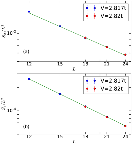
To determine the anomlous dimensions, i.e., the critical correlation-function exponents $\eta^{xy}_{\text{JQ}}$ and $\eta^{z}_{\text{JQ}}$ in Eq. (17), we analyze the system-size dependence of the squares of the easy-plane off-diagonal spin order parameter $M^{2}_{xy}(L)$ in Eq. (20) and dimer order parameter

$$D^{2}(L)=\frac{1}{2}\left(((D^{x}(L))^{2}+(D^{y}(L))^{2}\right),$$ (25)

where the $x$ and $y$ dimer operators are the appropriate Fourier transforms of Eqs. (14) corresponding to a columnar VBS;

$$D^{x}=\frac{1}{L^{2}}\sum_{i}(-1)^{x_{i}}D^{x}_{i},$$ (26a)

$$D^{x}=\frac{1}{L^{2}}\sum_{i}(-1)^{y_{i}}D^{y}_{i}.$$ (26b)

In the diagonal $S^{z}$ channel we study the system size dependence of the staggered magnetization

$$M^{2}_{z}=\frac{1}{L^{4}}\sum_{i,j}(-1)^{i+j}S^{z}_{i}S^{z}_{j}.$$ (27)

All these integrated correlation functions should scale as the correlation functions in Eq. (17) with the distance $|{\bf r}_{ij}|$ replaced by the system length $L$.

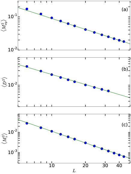
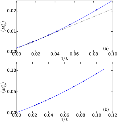
This dimer order parameter should be governed by the same exponent $\eta^{xy}_{\text{JQ}}$ as the off-diagonal spin order parameter if the predicted O(4) symmetry is manifested. In contrast, the diagonal magnetic order parameter is associated with a different (larger) anomalous dimension $\eta^{z}_{\text{JQ}}$, according to the table in Fig. 1. We have evaluated the order parameters at $q=0.620$, consistent with the value of $q_{c}$ determined in previous subsection. Results are shown in Fig. 3 for system sizes up to $L=32$ and $L=40$ for the dimer and spin order parameters, respectively. In Fig. 3(a,b) we show that $M^{2}_{xy}$ and $D^{2}$ can be fitted with the same exponent, $\eta^{xy}_{\text{JQ}}=0.13(3)$, while the fit to $M^{2}_{z}$ in Fig. 3(c) delivers a distinctively different exponent; $\eta^{z}_{\text{JQ}}=0.91(3)$.

V Results for the Bilayer Honeycomb model

In this section we present our numerical results on the continuous phase transition in the BH model, where an interaction-driven phase transition between a BSPT phase and a trivial Mott insulator is investigated via large-scale DQMC simulations He et al. (2016a, c, b) in the ground-state projector versionAssaad and Evertz (2008). Acting with the operator ${\rm e}^{-\Theta H}$ on a trial state (a Slater determinant) with the projection ’time’ $\Theta$ large enough for converging the finite system to its ground state, we simulated linear system sizes $L=12,15,18,21$ and $24$, with $\Theta=50$ for $L\leq 18$, $\Theta=55$ for $L=21$, and $\Theta=60$ for $L=24$. The imaginary-time discretization step was $\Delta\tau=0.05$, which is sufficiently small to not lead to any significant deviations of scaling behaviors from the $\Delta\tau=0$ limit.

V.1 The continuous topological phase transition

Figure 4: DQMC results for the BH model close to its phase transition. The derivative with respect to the coupling $V$ of (a) the kinetic energy density and (b) the total ground-state energy density for linear system sizes $L=6$, $9$ and $12$. Panel (c) shows the zero-frequency susceptibility of the O($4$) vector in the pairing channel for $L=6$, $9$, $12$, $15$, $18$. The dashed line indicates our estimated critical point $V_{c}=2.82(1)$.

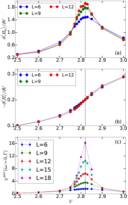
We first present simulation results supporting a continuous BSPT–Mott transition (as was also previously discussed in Ref. He et al. (2016a, b)). Figure 4(a) shows the derivative of the kinetic energy density of the BH Hamiltonian Eq. (4) with respect to the control parameter $V$ of the phase transition,

$$\frac{\partial\langle H_{\text{k}}\rangle}{\partial V}=-\frac{t}{N}\frac{\partial}{\partial V}\sum_{\langle ij\rangle}\langle c^{\dagger}_{i}c_{j}+\text{h.c.}\rangle.$$ (28)

Here a broad peak develops close to $V_{c}$, but there is no sign of a divergence, as would be expected at a first-order transition. Figure 4(b) shows the derivative of the ground state energy density, which can be conveniently evaluated by invoking the Hellmann-Feynman theorem;

$$\frac{\partial\langle H\rangle}{\partial V}=\Big{\langle}\frac{\partial H}{\partial V}\Big{\rangle}=\frac{1}{N}\sum_{i}\langle c_{i1\uparrow}^{\dagger}c_{i2\uparrow}c_{i1\downarrow}^{\dagger}c_{i2\downarrow}+\text{h.c.}\rangle.$$ (29)

For this derivative a first-order transition would lead to a sharp kink developing with increasing $L$ (corresponding to a real or avoided level crossing). The smooth behavior supports a continuous phase transition, though of course a very weak first-order transition would produce a visible singular behavior only for larger system sizes than we consider here.

To determine the phase-transition point $V_{c}$, we have further calculated the zero-frequency susceptibility of the O(4) vector (where we here take the on-site spin-singlet pairing operator), defined as

$$\chi^{\rm pair}(i\omega=0,\boldsymbol{\Gamma})=\int_{0}^{+\infty}S(\tau,\boldsymbol{\Gamma})d\tau,$$ (30)

where the dynamic pair-pair correlation function is defined as

$$S(\tau,\boldsymbol{\Gamma})=\frac{1}{L^{2}}\sum_{ij}e^{i\mathbf{k}\cdot(\mathbf{R}_{i}-\mathbf{R}_{j})}\frac{\langle\Delta_{i}^{\dagger}(\tau)\Delta_{j}+\Delta_{j}^{\dagger}(\tau)\Delta_{i}\rangle}{2},\\$$ (31)

where $k=0$ and $\Delta_{i}$ defined in Eq. (7). As demonstrated in Fig. 4(c), this quantity exhibits a sharp peak, as expected at a gapless critical point with power-law correlations in both space and time. The divergence is considerably slower than the $\propto$ space-time-volume behavior expected at a first-order transition. Due to the large computational effort needed for these DQMC simulations, we do not have a sufficient density of points close to $V_{c}$ to carry out a systematic analysis of the drift of the peak position, but the data nevertheless allow us to roughly estimate the convergence to the critical point $V_{c}/t=2.82(1)$.

Figure 5: (a) Excitation gaps computed from the imaginary-time decay of the O(4) vector across the BSPT-Mott transition for the BH model with $L=6,9,12,15,18$. A gap closing at $V_{c}=2.82t$ (vertical dashed line) is expected. (b) Finite-size scaling of $L\Delta_{O(4)}$ for $V/t=2.80,2.82,2.85$ vs the inverse system size. The behavior at $V/t=2.82$ indicates $z=1$. (c) Data collapse of the data in (a) according to the expected scaling form Eq. (32), yielding $\nu_{\text{BH}}=0.53(5)$ and $V_{c}/t=2.80(1)$.

V.2 O(4) gap and BH correlation-length exponent

We have also extracted the excitation gaps, $\Delta_{O(4)}$, corresponding to the $O(4)$ vectors defined in Eq. (7). According to Refs. He et al. (2016a, b) and Eq. (31), the O(4) gap is obtained from the imaginary-time decay of the dynamical O(4) vector correlation function, and, as discussed in Sec. II and Sec. III.1, O(4) bosonic modes are expected to become gapless (with power-law correlation) at the BSPT-Mott critical point. Results for $\Delta_{O(4)}$ as a function of $V/t$ for system sizes $L=6,9,12,15,18$ close to $V_{c}$ are presented in Fig. 5(a). As expected, $\Delta_{O(4)}$ from every system size $L$ exhibits a dip close to $V_{c}$, with the gap minimum decreasing with $L$ as expected with an emergent gapless point at $V_{c}$. In Fig. 5(b) we analyze the size dependence of the gap at three different coupling values; $V/t=2.80,2.82,2.85$. At $V/t=2.82$, $L\Delta_{O(4)}$ extrapolates linearly in $1/L$ to a nonzero value, showing that the leading behavior of $\Delta_{O(4)}$ at $V_{c}$ is $1/L$. This is in line with the expectation that the dynamic exponent $z=1$ at the BSPT-Mott transition (and is required also for the proposed duality). The behaviors of $\Delta_{O(4)}L$ at $V/t=2.80,2.85$ indicate eventual divergencies when $L\to\infty$, as expected on either side of the quantum critical point. This constitutes strong evidence of a continuous transition, instead of a first-order transition at which one instead expects a gap closing exponentially fast.

To extract the correlation-length exponent $\nu_{\text{BH}}$, we have performed data collapse with the $O(4)$ gap away from the critical point, as shown in Fig. 4(c). Here we focus on the regime $V>V_{c}$, where we find less scaling corrections than for $V<V_{c}$ and an almost perfect data-collapse according to the expected quantum-critical form

$$\Delta_{O(4)}L=f[(V/V_{c}-1)L^{1/\nu_{\rm BH}}].$$ (32)

Treating both $\nu_{\text{BH}}$ and $V_{c}$ as free parameters, the best data collapse delivers $\nu_{\rm BH}=0.53(5)$ and $V_{c}/t=2.80(1)$. This value of $V_{c}$ agrees quite well with the result $V_{c}=2.82(1)$ estimated roughly from the susceptibility peak in Fig. 4, adding further credence to the analysis of the critical point even with the rather limited range of system sizes accessible (as compared with the EPJQ model). Moreover, since we already determined $\eta^{z}_{\text{JQ}}=0.91(3)$ in the EPJQ model, we can use the duality relationship in Eq. (18a) to predict that the correlation-length exponent of the BH model should be $\nu_{\text{BH}}\sim 0.49(2)$, which is fully consistent the number determined from the $O(4)$ gap.

V.3 Anomalous dimensions

Finally, we study the critical equal-time correlations in the BH model. Here we have used $V=2.817$ for the longest simulations. This value is within the error bars of the critical value $V_{c}=2.82(1)$ and, as we will also show, there are no statistically detectable differences between data at $V=2.820$ and $2.817$ for the quantities studied in this subsection.

Using one of the components of the $O(4)$ order parameter, $\langle\Delta^{\dagger}_{i}\Delta_{j}\rangle$ with $\Delta_{i}$ defined in Eq. (7), we again construct a squared order parameter. We can use the susceptibility Eq. (31) to define a corresponding equal-time spatially-integrated correlation function,

$$\frac{S_{\Delta}}{L^{2}}=\frac{S(\tau=0,{\bf\Gamma})}{L^{2}},$$ (33)

where the normalization gives the same scaling behaviors as in Eq. (16) with the distance $|{\bf r}_{ij}|$ replaced by $L$. The analysis illustrated in Fig. 6(a) indicates a very good power-law scaling, with deviations seen only for the smallest system size (which we exclude from the fit). The fit delivers the exponent $\eta_{\rm BH}^{\Delta}=0.10(1)$, which is fully consistent with the EPJQ exponent $\eta^{xy}_{\text{JQ}}=0.10(2)$ obtained in Sec. IV.2. Hence, the duality relation Eq. (18c) is satisfied to within the statistical errors.

In principle the anomalous dimension can also be obtained from the susceptibility in Fig. 5(c). Standard scaling arguments give that the peak height of a generic susceptibility $\chi$ should scale as $\chi_{\rm peak}\propto L^{2-\eta}$ (when the dynamic exponent $z=1$). We find that the peak in $\chi^{\rm pair}$ scales approximately as $L^{2}$, i.e., $\eta^{\Delta}$ is very small, but here there appears to be significant scaling corrections. Moreover, there is large variation of the values for the largest size, $L=18$, close to the critical point, and we would need additional points to reliably estimate the peak value. We therefore cannot obtain an independent meaningful estimate for $\eta^{\Delta}_{\rm BH}$ from these data.

Figure 6: Analysis of the anomalous dimensions $\eta^{\Delta}_{BH}$ and $\eta^{\rho}_{\text{BH}}$ of the BH model from squared order parameters close to the critical point. Only the $V=2.817$ data points for each quantity are used in the fits, and the three points for $V=2.82$ do not exhibit any deviations from the $V=2.817$ values within the error bars. (a) shows the $O(4)$ order parameter defined in Eq. (33). A power-law fit (straight line on the log-log scale) to the $L\geq 15$ data delivers the exponent $\eta^{\Delta}_{\text{BH}}=0.10(1)$. (b) The pair-density order parameter Eq. (34). Here the power-law fit works well for all system sizes and we obtain $\eta^{\rho}_{\text{BH}}=1.00(1)$.

We next test the duality relation Eq. (18b). With $\nu^{xy}_{\text{JQ}}=0.48(3)$ obtained in Sec. IV.1 we expect $\eta^{\rho}_{\text{BH}}\approx 1$. Further, according to Ref. Karthik and Narayanan (2016), the exponent $\eta^{\rho}_{\text{BH}}$ should be equal to the anomalous mass dimension $\eta_{\text{QED}}$ of $N=2$ QED, for which the value $\eta_{\text{QED}}=1.0(2)$ was obtained from Monte Carlo simulations. Thus, we already have good consistency following from the predicted duality between $\eta_{\text{QED}}$ and $\nu^{xy}_{\text{JQ}}$. Turning to the more direct test with the BH model, in Fig. 6(b) we plot the squared order parameter corresponding to the pair-density,

$$\frac{S_{\rho}}{L^{2}}=\frac{1}{L^{4}}\sum_{i,j}\langle\rho_{i\uparrow}\rho_{i\downarrow}\rho_{j\uparrow}\rho_{j\downarrow}\rangle.$$ (34)

For this quantity, as shown in Fig. 6(b), all five system sizes available give results fully consistent with a power-law decay, with no statistically visible scaling corrections. The fit to the five data points gives the anomalous dimension $\eta^{\rho}_{\text{BH}}=1.00(1)$, which is consistent with both $\eta_{\text{QED}}$ and $\nu^{xy}_{\text{JQ}}$, but with a significantly smaller statistical error. Thus, the duality relation in Eq. (18b) is also confirmed to within error bars.

It is remarkable that the BH model actually seems to give better results (smaller error bars) for the anomalous dimensions than the EPJQ model, even though system lengths roughly twice as large were used for the latter. The reason is that the statistical errors on the raw data are smaller in the DQMC simulations. It is still possible that there are scaling corrections present that are not clearly visible with such a small range of system sizes, and there may then be some corrections to the exponents beyond the purely statistical error bars (one standard deviation) reported above. The EPJQ results are important in this regard as they seem to show no significant corrections even with the considerably larger range of system sizes. The lack of significant corrections is also supported by the good agreement between the non-reivial BH and EPJQ exponents, as predicted by the duality conjecture.

VI Discussion

We have performed detailed numerical tests on the recently proposed duality summarized by the predicted exponent relationships between the BH and EPJQ models in Eq. (18). The relationships were confirmed within statistical precision at the level of a few percent in the values of the critical exponents. The thus confirmed duality of the underlying low-energy quantum field theories, Eq. (1), is of great importance and interest in condensed-matter physics, because it relates two seemingly different quantum phase transitions that have been individually under intense studies during the past several years: the bosonic topological phase transition and the easy-plane deconfined quantum phase transition. The duality was derived using the more basic dualities between field theories that involve only one flavor of matter field, and sometimes also a Chern-Simons term of the dynamical gauge field.

As a consequence of confirming the particular relationship between critical exponents, our study also provides quantitative evidence for the underlying basic dualities for theories with one flavor of matter field Son (2015); Wang and Senthil (2016a, 2015, b); Metlitski and Vishwanath (2016); Seiberg et al. (2016). These basic dualities supported by our work represent a significant step in our understanding of $(2+1)D$ conformal field theories. They also form the foundation of a large number of other recently proposed dualities Xu and You (2015); Mross et al. (2016); Hsin and Seiberg (2016); Karch and Tong (2016); Cheng and Xu (2016); Karch et al. (2017); Benini et al. (2017); Hsiao and Son (2017); Mross et al. (2017). Moreover, they lend support to many other dualities that follow from the same logic and reasoning, such as the duality of Majorana fermions discussed in Refs. Metlitski et al. (2016); Aharony et al. (2017).

To follow up on our results and insights presented here, additional numerical investigations are called for to check other predictions made within these proposed dualities. For example, in Ref. Wang et al. (2017) it was proposed that the Gross-Neveu fixed point of the $N=2$ QED is dual to the SU(2) version of the NCCP¹ model, and also has an emergent SO($5$) symmetry. This symmetry has recently been discussed within SU(2) deconfined quantum-criticality as well, and quite convincing results pointing in this direction were seen in a three-dimensional loop model Nahum et al. (2015b). Scaling with the same anomalous dimension for both spin and dimer correlators had also been observed already some time ago in the SU(2) $J$-$Q$ model Sandvik (2012). Although we have identified the $N=2$ QED as the bosonic topological phase transition in our bilayer honeycomb lattice model, we have so far been unable to find the corresponding Gross-Neveu fixed point. Identifying the additional interactions that will be required to drive this transition in the BH model is an important topic for forther research.

Following previous computational studies of deconfined quantum phase transition with SU($2$) spin-rotation symmetry in $J$-$Q$ models Sandvik (2007); Lou et al. (2009); Shao et al. (2016), we have here identified a lattice model—the EPJQ model—hosting a continuous phase transition between the $U(1)$ (planar) Néel and VBS states. The fact that this phase transition is continuous is in itself an important discovery, given that U($1$) deconfined-quantum criticality had essentially been declared non-existent, due to unexplained hints of first-order transitions in some other planar models and what seems like definite proofs in other cases Kuklov et al. (2008); D’Emidio and Kaul (2016); Geraedts and Motrunich (2017). Here (as further discussed in Appendix B) we have shown that the EPJQ model defined in Eq. (11) can host first-order or continuous transitions, depending on the degree of spin-anisotropy parametrized by the Ising coupling $\Delta$ in Eq. (11). At $\Delta=1/2$, we find scaling behaviors with apparently much less influence of scaling corrections than in the SU($2$) $J$-$Q$ model at its deconfined critical point Shao et al. (2016), i.e., the leading correction exponent $\omega$ is much larger in the EPJQ model. Interestingly, in both cases the correlation-length exponent is unusually small, close to $1/2$, while well-studied transitions such as the O($N$) transitioins in three dimensions have exponents close to $2/3$. Given its small scaling corrections and likely tricritical point between $\Delta=1/2$ and $\Delta=1$, the EPJQ model opens doors for future detailed studies on exotic phase transitions beyond the Landau paradigm.

Appendix A Crossing-point analysis

To determine the critical point and the critical exponents in an unbiased manner, we adopt the crossing-point analysis applied and tested for 2D Ising and SU(2) $J$-$Q$ models in Ref. Shao et al. (2016). Such analysis can be further traced back to Fisher’s ”phenomenological renormalization”, which was first numerically tested with transfer-matrix results for the Ising model in Ref. Luck (1985). Ref. Shao et al. (2016) presented systematic procedures for a statistically sound application of these techniques with Monte Carlo data. For easy reference we here summarize how we have adapted the method to the EPJQ model studied in this paper. For the BH model, due to the much larger computational cost of the DQMC simulations, we do not have data for enough system sizes to carry out the analysis in this way, and we instead applied other scaling methods in Sec. V.

Considering a generic critical point, with $\delta=q-q_{c}$ defined as the distance to the critical point $q_{c}$—for example, here $q$ can be the control parameter $q=Q/(J+Q)$ that we used for the EPJQ model or it could be $T-T_{c}$ for a finite-temperature transition. For any observable $O$, the standard finite-size scaling form is

$$O(\delta,L)=L^{-{\kappa}/{\nu}}f(\delta L^{{1}/{\nu}},\lambda L^{-\omega}),$$ (35)

where we, for the sake of simplicity, only consider one irrelevant field $\lambda$ and the corresponding subleading exponent $\omega$. At the critical point, one can Taylor expand the scaling function,

$$O(\delta,L)=L^{-{\kappa}/{\nu}}(a_{0}+a_{1}\delta L^{{1}/{\nu}}+b_{1}L^{-\omega}+\cdots).$$ (36)

If one now takes two system sizes, e.g., $L_{1}=L$ and $L_{2}=rL$ $(r>1)$, and trace the crossing points $\delta^{*}(L)$ of curves $O(\delta,L_{1})$ and $O(\delta,L_{2})$ versus $\delta$, one finds

$$\delta^{*}(L) = \frac{a_{0}}{a_{1}}\frac{1-r^{-{\kappa}/{\nu}}}{r^{{(1-\kappa)}/{\nu}-1}}L^{-{1}/{\nu}}$$ (37)

$$+\frac{b_{1}}{a_{1}}\frac{1-r^{-({\kappa}/{\nu}+\omega})}{r^{{(1-\kappa)}/{\nu}-1}}L^{-({1}/{\nu}+\omega)}.$$

Now if the quantity $O$ is asymptotically size-independent (dimensionless) at the critical point, for example the Binder cumulant (which we write here with a constant and factor corresponding to a planar vector order parameter),

$$U=2\left(1-\frac{\langle m^{4}_{xy}\rangle}{2\langle m^{2}_{xy}\rangle^{2}}\right)$$ (38)

then the corresponding exponent $\kappa=0$, the first term in Eq. (37) with $O=U$ vanishes, and we obtain the following form for the size-dependent crossing point $\delta^{*}(L)$:

$$\delta^{*}(L)=q^{*}_{c}(L)-q_{c}\propto L^{-({1}/{\nu}+\omega)},$$ (39)

hence the shift of the finite-size critical point $q^{*}_{c}(L)$ is approaching the asymptotic value $q_{c}$ as $L^{-({1}/{\nu}+\omega)}$.

In practice, one can interpolate within a set of points for each system size by a fitted polynomial, e.g., of cubic or quadratic order, and then use these polynomials to find the crossing points. This is illustrated in Fig 7. Error bars can be obtained by repeating the fits multiple times to data with Gaussian-distributed noise added. The scaling behavior of $q_{c}$ predicted by Eq. (39) can be clearly seen in Fig. 2(b) of the main text, from which the result ${1}/{\nu}+\omega=4.0(2)$ for the EPJQ model was obtained.

In addition to obtaining $q^{*}_{c}$ and the exponent combination $1/\nu+\omega$ from the crossing points of the cumulant (or, in principle, some other dimensionless quantity), one can also use the value $U^{*}_{c}$ of the quantity at $q^{*}_{c}$, as well as the derivatives at $q^{*}_{c}$, to acquire $\nu$ and $\omega$ independently. We next discuss the derivations underlying these forms.

By inserting $\delta^{*}(L)$ into Eq. (36), one can obtain the value of observable at the the finite-size critical point (or, more precisely, the critical point depending on the two sizes, $L$ and $rL$) $q^{*}_{c}(L)$. It scales as

$$O^{*}(L)=L^{-{\kappa}/{\nu}}(a+bL^{-\omega}+\cdots).$$ (40)

Again, for a dimensionless quantity ($\kappa=0$) such as $U$, the deviation of the value at the crossing point from the value in the thermodynamic limit vanishes with increasing size according to $U^{*}_{c}(L)-U_{c}\propto L^{-\omega}$, an example of which can be seen in Fig. 2(c) of the main text—in this case the power-law fit gave the value $\omega=2.3(1)$ of the subleading exponent.

Figure 7: Example of finite-size crossing points $q_{c}^{*}(L)$,$U_{c}^{*}(L)$ of the Binder cumulant, here for the EPJQ model with $L=16$ and $L=32$. The date are here fitted to third-order polynomials. The crossing point and derivatives at the crossing point can be determined from the fitted polynomials.

The last step of the analysis of the single dimensionless quantity is to determine $\nu$ in an independent manner. To this end, one can expand the quantity $U$ (or any other dimensionless quantity) close to the critical point,

$$U(\delta,L)=a_{0}+a_{1}\delta L^{{1}/{\nu}}+b_{1}L^{-\omega}+c_{1}\delta L^{{1}/{\nu}-\omega}+\cdots$$ (41)

and take the derivative $U^{\prime}(\delta,L)$ with respect of $\delta$ (in practice with respect to $q$);

$$U^{\prime}(\delta,L)=a_{1}L^{{1}/{\nu}}+c_{1}L^{{1}/{\nu}-\omega}+\cdots.$$ (42)

Again, we take two system sizes $L_{1}=L$ and $L_{2}=rL$, and at the crossing point $\delta^{*}(L)$ of the two curves for these system sizes one has

$$U^{\prime}(\delta^{*},L) = a_{1}L^{{1}/{\nu}}+c_{1}L^{{1}/{\nu}-\omega}$$

$$U^{\prime}(\delta^{*},rL) = a_{1}(rL)^{{1}/{\nu}}+c_{1}(rL)^{{1}/{\nu}-\omega}.$$ (43)

Here we can take the difference of the logarithms of the two equations and obtain,

$$\ln\left(\frac{U^{\prime}(\delta^{*},rL)}{U^{\prime}(\delta^{*},L)}\right)=\frac{1}{\nu}\ln(r)+dL^{-\omega}+\cdots,$$ (44)

or, in other words, one can define a finite-size estimate of the correlation-length exponent $\nu^{*}(L)$ from the finite-size crossing point as,

$$\frac{1}{\nu^{*}(L)}=\frac{1}{\ln(r)}\ln\left(\frac{U^{\prime}(\delta^{*},rL)}{U^{\prime}(\delta,L)}\right).$$ (45)

It can be seen that Eq. (45) approaches the thermodynamic limit correlation-length exponent $\nu$ at the rate ${1}/{\nu^{*}(L)}-{1}/{\nu}=gL^{-\omega}+\cdots$. This behavior is seen nicely in Fig. 2(d), where the extrapolation to infinite size gave $\nu^{xy}_{\text{JQ}}=0.48(2)$.

Figure 8: Crossing-point analysis of the extreme, $\Delta=1$, version of the EPJQ model, Eq.  (46). (a) The magnetic Binder cumulant versus the coupling $Q$ in the neighborhood of the phase transition. (b) Size dependence of the critical point defined as the crossing point of $U$ vs $Q$ for system sizes $L$ and $2L$, with a power-law fit giving $Q_{c}=1.732(2)$. (c) The cumulant evaluated at the crossing points. Here it is not clear whether the asymptotic behavior has been reached, and we refrain from carrying out a fit. (d) The finite-size correlation length. Here as well we do not present any fit, as the asymptotic behavior is not yet clear.

In principle one can also combine the above method for a dimensionless quantity with some other quantity $A$, e.g., an order parameter or a long-distance correlation function. Interpolating the data for two system sizes, $A(L)$ and $A(rL)$ at the crossing point of the dimensionless quantity, one can take the logarithm of the ratio and analyze it in a manner similar to the slope-estimate of $1/\nu$, to yield a series of finite-size estimates for the power-law governing the size dependence of $A$. This method circumvents the need to know the critical-point value exactly. In practice, since $q_{c}$ converges fast, it is also appropriate to just use this value and analyze the size-dependence of the quantity $A$ at this fixed coupling value $q=q_{c}$, as we did in the main text.

Appendix B Fully planar EPJQ model

In the main text we discussed the XYAFM–VBS transition at a fixed anisotropy parameter $\Delta=1/2$ of the EPJQ model. We here provide some more information on the dependence on $\Delta$.

Figure 9: Comparison of the XY magnetization squared of the $\Delta=1/2$ and $\Delta=1$ EPJQ models at their respective critical points. In (a) fits indicating a finite order parameter in the thermodynamic limit are indicated, with the dashed line corresponding to a purely linear correction and the solid curve to a quadratic form. In (b) a second-order fit is shown. The extrapolated value at $L=\infty$ is $0$ to within two error bars of the parameter obtained from the fit.

In the extreme planar limit $\Delta\to 1$ of Eq. (11) we have no $S^{z}S^{z}$ $J$-term and the Hamiltonian is

$$H_{\text{JQ}}=J\sum_{\langle ij\rangle}(S^{x}_{i}S^{x}_{j}+S^{y}_{i}S^{y}_{j})+Q\hskip-5.69054pt\sum_{\langle ijklmn\rangle}\hskip-5.69054ptD_{ij}D_{kl}D_{mn}.$$ (46)

We have analyzed SSE-QMC results for this model in the same way as we did for $\Delta=1/2$ in the main text, using a crossing-point analysis. The results of this analysis show a distinctively different behavior for $\Delta=1$, pointing to a first-order transition in this case. Results for the $L$-dependent quantities based on the XY Binder cumulant are shown in Fig. 8. As an aside, we mention here that for the model in Eq. (46) the off-diagonal spin correlations can be measured as diagonal correlations upon performing a basis rotation with the $z$ spin components transformed into the $x$ components, and vice versa. Simulating the system with SSE-QMC in this rotated basis speeds up the simulations of this variant of the model over those for generic $\Delta<1$. We therefore have results for larger system sizes in this case.

It is clear from Fig. 8 that we can obtain a good estimate of the critical point, but the cumulant itself and the correlation-length exponent do not exhibit the clear-cut power-law corrections of the type that we saw for the $\Delta=1/2$ model in Sec. IV. The fact that $1/\nu^{*}$ is larger than $3$ suggests that the transition may actually be of first order in this case. If so, we would expect the values to eventually tend exactly to $3$, and the data are consistent with this behavior.

If the transition indeed is of first order, the order parameter should be non-zero at the transition point, reflecting coexistence of the magnetic and non-magnetic phases. Indeed, as shown in Fig. 9(a), an extrapolation using a trivial $1/L$ correction, as expected asymptotically for a 2D system breaking a continuous symmetry, indicates a clearly non-zero value in the thermodynamic limit. The extrapolated value only changes slightly if a higher-order ($1/L^{2}$) correction is added (also expected if the order parameter is non-vanishing). In contrast, as shown in Fig. 9(b) the data for the $\Delta=1/2$ model are fully consistent with no magnetization in the thermodynamic limit. Here the polynomial fit is strictly not correct, since a non-trivial power is expected at the critical point (which we confirmed in the main paper), but the extrapolation nevertheless indicates consistency with a vanishing order parameter at the transition in this case.

These results strongly suggest that there is a tricritical point separating a continuous and first-order transition in the EPJQ model somewhere between $\Delta=1/2$ and $\Delta=1$, which we plan to investigate further in a future study.

References

- Kramers and Wannier (1941) H. A. Kramers and G. H. Wannier, Phys. Rev. 60, 252 (1941).
- Kogut (1979) J. B. Kogut, Rev. Mod. Phys. 51, 659 (1979).
- Savit (1980) R. Savit, Rev. Mod. Phys. 52, 453 (1980).
- Peskin (1978) M. E. Peskin, Annals of Physics 113, 122 (1978).
- Dasgupta and Halperin (1981) C. Dasgupta and B. I. Halperin, Phys. Rev. Lett. 47, 1556 (1981).
- Fisher and Lee (1989) M. P. A. Fisher and D. H. Lee, Phys. Rev. B 39, 2756 (1989).
- Note (1) Here the term ”noncompact” means that the U(1) gauge flux is a conserved quantity.
- Montonen and Olive (1977) C. Montonen and D. Olive, Physics Letters B 72, 117 (1977).
- Seiberg (1995) N. Seiberg, Nuclear Physics B 435, 129 (1995).
- Seiberg and Witten (1994a) N. Seiberg and E. Witten, Nuclear Physics B 426, 19 (1994a).
- Seiberg and Witten (1994b) N. Seiberg and E. Witten, Nuclear Physics B 431, 484 (1994b).
- Cardy and Rabinovici (1982) J. L. Cardy and E. Rabinovici, Nuclear Physics B 205, 1 (1982).
- Cardy (1982) J. L. Cardy, Nuclear Physics B 205, 17 (1982).
- Witten (1995) E. Witten, Selecta Math. 1, 383 (1995).
- Coleman (1975) S. Coleman, Phys. Rev. D 11, 2088 (1975).
- Mandelstam (1975) S. Mandelstam, Phys. Rev. D 11, 3026 (1975).
- Luther and Peschel (1974) A. Luther and I. Peschel, Phys. Rev. B 9, 2911 (1974).
- Witten (1984) E. Witten, Commun. Math. Phys. 92, 455 (1984).
- Giamarchi (2004) T. Giamarchi, Quantum Physics in One Dimension, International Series of Monogr (Clarendon Press, 2004).
- Potter et al. (2016) A. C. Potter, C. Wang, M. A. Metlitski, and A. Vishwanath, ArXiv e-prints (2016), arXiv:1609.08618 [cond-mat.str-el] .
- Wang et al. (2017) C. Wang, A. Nahum, M. A. Metlitski, C. Xu, and T. Senthil, ArXiv e-prints (2017), arXiv:1703.02426 [cond-mat.str-el] .
- Slagle et al. (2015) K. Slagle, Y.-Z. You, and C. Xu, Phys. Rev. B 91, 115121 (2015).
- He et al. (2016a) Y.-Y. He, H.-Q. Wu, Y.-Z. You, C. Xu, Z. Y. Meng, and Z.-Y. Lu, Phys. Rev. B 93, 115150 (2016a).
- Wu et al. (2016) H.-Q. Wu, Y.-Y. He, Y.-Z. You, T. Yoshida, N. Kawakami, C. Xu, Z. Y. Meng, and Z.-Y. Lu, Phys. Rev. B 94, 165121 (2016).
- Grover and Vishwanath (2013a) T. Grover and A. Vishwanath, Phys. Rev. B 87, 045129 (2013a).
- Lu and Lee (2014) Y.-M. Lu and D.-H. Lee, Phys. Rev. B 89, 195143 (2014).
- Sandvik (2007) A. W. Sandvik, Phys. Rev. Lett. 98, 227202 (2007).
- Senthil et al. (2004a) T. Senthil, A. Vishwanath, L. Balents, S. Sachdev, and M. P. A. Fisher, Science 303, 1490 (2004a).
- Senthil et al. (2004b) T. Senthil, L. Balents, S. Sachdev, A. Vishwanath, and M. P. A. Fisher, Phys. Rev. B 70, 144407 (2004b).
- Senthil and Fisher (2006) T. Senthil and M. P. A. Fisher, Phys. Rev. B 74, 064405 (2006).
- Shao et al. (2016) H. Shao, W. Guo, and A. W. Sandvik, Science 352, 213 (2016).
- Son (2015) D. T. Son, Phys. Rev. X 5, 031027 (2015).
- Wang and Senthil (2016a) C. Wang and T. Senthil, Phys. Rev. X 6, 011034 (2016a).
- Wang and Senthil (2015) C. Wang and T. Senthil, Phys. Rev. X 5, 041031 (2015).
- Wang and Senthil (2016b) C. Wang and T. Senthil, Phys. Rev. B 93, 085110 (2016b).
- Metlitski and Vishwanath (2016) M. A. Metlitski and A. Vishwanath, Phys. Rev. B 93, 245151 (2016).
- Seiberg et al. (2016) N. Seiberg, T. Senthil, C. Wang, and E. Witten, Annals of Physics 374, 395 (2016).
- Kachru et al. (2017) S. Kachru, M. Mulligan, G. Torroba, and H. Wang, Phys. Rev. Lett. 118, 011602 (2017).
- Kachru et al. (2016) S. Kachru, M. Mulligan, G. Torroba, and H. Wang, Phys. Rev. D 94, 085009 (2016).
- Mross et al. (2016) D. F. Mross, J. Alicea, and O. I. Motrunich, Phys. Rev. Lett. 117, 016802 (2016).
- Note (2) A more precise form of the dual D QED is given in Ref. \rev@citealpseiberg1.
- Xu and You (2015) C. Xu and Y.-Z. You, Phys. Rev. B 92, 220416 (2015).
- Motrunich and Vishwanath (2004) O. I. Motrunich and A. Vishwanath, Phys. Rev. B 70, 075104 (2004).
- Karch and Tong (2016) A. Karch and D. Tong, Phys. Rev. X 6, 031043 (2016).
- Hsin and Seiberg (2016) P.-S. Hsin and N. Seiberg, Journal of High Energy Physics 2016, 95 (2016).
- Grover and Vishwanath (2013b) T. Grover and A. Vishwanath, Phys. Rev. B 87, 045129 (2013b).
- Chen et al. (1993) W. Chen, M. P. A. Fisher, and Y.-S. Wu, Phys. Rev. B 48, 13749 (1993).
- Sandvik et al. (2002) A. W. Sandvik, S. Daul, R. R. P. Singh, and D. J. Scalapino, Phys. Rev. Lett. 89, 247201 (2002).
- Lou et al. (2009) J. Lou, A. W. Sandvik, and N. Kawashima, Phys. Rev. B 80, 180414 (2009).
- Sen and Sandvik (2010) A. Sen and A. W. Sandvik, Phys. Rev. B 82, 174428 (2010).
- Sandvik (2010) A. W. Sandvik, Phys. Rev. Lett. 104, 177201 (2010).
- Nahum et al. (2011) A. Nahum, J. T. Chalker, P. Serna, M. Ortuño, and A. M. Somoza, Phys. Rev. Lett. 107, 110601 (2011).
- Harada et al. (2013) K. Harada, T. Suzuki, T. Okubo, H. Matsuo, J. Lou, H. Watanabe, S. Todo, and N. Kawashima, Phys. Rev. B 88, 220408 (2013).
- Pujari et al. (2013) S. Pujari, K. Damle, and F. Alet, Phys. Rev. Lett. 111, 087203 (2013).
- Pujari et al. (2015) S. Pujari, F. Alet, and K. Damle, Phys. Rev. B 91, 104411 (2015).
- Nahum et al. (2015a) A. Nahum, J. T. Chalker, P. Serna, M. Ortuño, and A. M. Somoza, Phys. Rev. X 5, 041048 (2015a).
- Nahum et al. (2015b) A. Nahum, P. Serna, J. T. Chalker, M. Ortuño, and A. M. Somoza, Phys. Rev. Lett. 115, 267203 (2015b).
- Kuklov et al. (2008) A. B. Kuklov, M. Matsumoto, N. V. Prokof’ev, B. V. Svistunov, and M. Troyer, Phys. Rev. Lett. 101, 050405 (2008).
- Geraedts and Motrunich (2012) S. D. Geraedts and O. I. Motrunich, Phys. Rev. B 85, 045114 (2012).
- D’Emidio and Kaul (2016) J. D’Emidio and R. K. Kaul, Phys. Rev. B 93, 054406 (2016).
- D’Emidio and Kaul (2017) J. D’Emidio and R. K. Kaul, Phys. Rev. Lett. 118, 187202 (2017).
- Karthik and Narayanan (2016) N. Karthik and R. Narayanan, Phys. Rev. D 94, 065026 (2016).
- He et al. (2016b) Y.-Y. He, H.-Q. Wu, Z. Y. Meng, and Z.-Y. Lu, Phys. Rev. B 93, 195164 (2016b).
- Meng et al. (2010) Z. Y. Meng, T. C. Lang, S. Wessel, F. F. Assaad, and A. Muramatsu, Nature 464, 847 (2010).
- Meng et al. (2014) Z. Y. Meng, H.-H. Hung, and T. C. Lang, Modern Physics Letters B 28, 1430001 (2014).
- Kane and Mele (2005) C. L. Kane and E. J. Mele, Physical Review Letter 95, 226801 (2005).
- You et al. (2016) Y.-Z. You, Z. Bi, D. Mao, and C. Xu, Phys. Rev. B 93, 125101 (2016).
- You and You (2016) Y. You and Y.-Z. You, Phys. Rev. B 93, 195141 (2016).
- Sandvik (1999) A. W. Sandvik, Phys. Rev. B 59, R14157 (1999).
- Syljuåsen and Sandvik (2002) O. F. Syljuåsen and A. W. Sandvik, Phys. Rev. E 66, 046701 (2002).
- Jin et al. (2012) S. Jin, A. Sen, and A. W. Sandvik, Phys. Rev. Lett. 108, 045702 (2012).
- He et al. (2016c) Y.-Y. He, H.-Q. Wu, Z. Y. Meng, and Z.-Y. Lu, Phys. Rev. B 93, 195163 (2016c).
- Assaad and Evertz (2008) F. F. Assaad and H. G. Evertz, in Computational Many-Particle Physics, Lecture Notes in Physics, Vol. 739, edited by H. Fehske, R. Schneider, and A. Weiße (Springer Berlin Heidelberg, 2008) pp. 277–356.
- Cheng and Xu (2016) M. Cheng and C. Xu, Phys. Rev. B 94, 214415 (2016).
- Karch et al. (2017) A. Karch, B. Robinson, and D. Tong, Journal of High Energy Physics 2017, 17 (2017).
- Benini et al. (2017) F. Benini, P.-S. Hsin, and N. Seiberg, arXiv:1702.07035 (2017).
- Hsiao and Son (2017) W.-H. Hsiao and D. T. Son, arXiv:1705.01102 (2017).
- Mross et al. (2017) D. F. Mross, J. Alicea, and O. I. Motrunich, arXiv:1705.01106 (2017).
- Metlitski et al. (2016) M. A. Metlitski, A. Vishwanath, and C. Xu, arXiv:1611.05049 (2016).
- Aharony et al. (2017) O. Aharony, F. Benini, P.-S. Hsin, and N. Seiberg, Journal of High Energy Physics 2017, 72 (2017).
- Sandvik (2012) A. W. Sandvik, Phys. Rev. B 85, 134407 (2012).
- Geraedts and Motrunich (2017) S. D. Geraedts and O. I. Motrunich, ArXiv e-prints (2017), arXiv:1705.06308 [cond-mat.str-el] .
- Luck (1985) J. M. Luck, Phys. Rev. B 31, 3069 (1985).