Trade-off shapes diversity in eco-evolutionary dynamics

Abstract

We introduce an Interaction and Trade-off based Eco-Evolutionary Model (ITEEM), in which species are competing for common resources in a well-mixed system, and their evolution in interaction trait space is subject to a life-history trade-off between replication rate and competitive ability. We demonstrate that the strength of the trade-off has a fundamental impact on eco-evolutionary dynamics, as it imposes four phases of diversity, including a sharp phase transition. Despite its minimalism, ITEEM produces without further ad hoc features a remarkable range of observed patterns of eco-evolutionary dynamics. Most notably we find self-organization towards structured communities with high and sustainable diversity, in which competing species form interaction cycles similar to rock-paper-scissors games.

Our intuition separates the time scales of fast ecological and slow evolutionary dynamics, perhaps because we experience the former but not the latter. However, there is increasing experimental evidence that this intuition is wrong Messer et al. (2016); Hendry (2016); Carrol et al. (2007). This insight is challenging both ecological and evolutionary theory, but has also sparked efforts towards unified eco-evolutionary theories Carrol et al. (2007); Fussmann et al. (2007); Schoener (2011); Ferriere and Legendre (2012); Moya-Laraño et al. (2014); Hendry (2016). Here we contribute a new, minimalist model to these efforts, the Interaction and Trade-off based Eco-Evolutionary Model (ITEEM).

The first key idea underlying ITEEM is that interactions between organisms, mainly competitive interactions, are central to ecology and to evolution Allesina and Levine (2011); Barraclough (2015); Weber et al. (2017); Coyte et al. (2015). This insight has inspired work on interaction network topology Knebel et al. (2013); Tang et al. (2014); Melo and Marroig (2015); Laird and Schamp (2015); Coyte et al. (2015), and on how these networks evolve and shape diversity Ginzburg et al. (1988); Solé (2002); Tokita and Yasutomi (2003); Drossel et al. (2001); Loeuille and Loreau (2009). The second key component of the model is a trade-off between interaction traits and replication rate: better competitors replicate less. Such trade-offs, probably rooted in differences of energy allocation between life-history traits, have been observed across biology Stearns (1989); Kneitel and Chase (2004); Agrawal et al. (2010); Maharjan et al. (2013); Ferenci (2016), and they were found to be important for emergence and stability of diversity Rees (1993); Bonsall (2004); de Mazancourt and Dieckmann (2004); Ferenci (2016).

We show here that ITEEM dynamics closely resembles observed eco-evolutionary dynamics, such as sympatric speciation Drossel and McKane (2000); Coyne (2007); Bolnick and Fitzpatrick (2007); Herron and Doebeli (2013), emergence of two or more levels of differentiation similar to phylogenetic structures Barraclough et al. (2003), large and complex biodiversity over long times Herron and Doebeli (2013); Kvitek and Sherlock (2013), evolutionary collapses and extinctions Kärenlampi (2014); Solé (2002), and emergence of cycles in interaction networks that facilitate species diversification and coexistence Mathiesen et al. (2011); Bagrow and Brockmann (2013); Allesina and Levine (2011); Laird and Schamp (2015). Interestingly, the model shows a unimodal (“humpback”) behavior of diversity as function of trade-off, with a critical trade-off at which biodiversity undergoes a phase transition, a behavior observed in nature Smith (2007); Vallina et al. (2014); Nathan et al. (2016).

ITEEM has $N_{s}$ sites of undefined spatial arrangement (well-mixed system), each providing resources for one organism. We start an eco-evolutionary simulation with individuals of a single strain occupying a fraction of the $N_{s}$ sites. Note that in the following we use the term strain for a set of individuals with identical traits. In contrast, a species is a cluster of strains with some diversity (cluster algorithm described in Supplemental Material SM-1 SM ).

At every generation or time step $t$, we try $N_{ind}(t)$ (number of individuals) replications of randomly selected individuals. Each selected individual of a strain $\alpha$ can replicate with rate $r_{\alpha}$, with its offspring randomly mutated with rate $\mu$ to new strain $\alpha^{\prime}$. An individual will vanish if it has reached its lifespan, drawn at birth from a Poisson distribution with overall fixed mean lifespan $\lambda$.

Each newborn individual is assigned to a randomly selected site. If the site is empty, the new individual will occupy it. If the site is already occupied, the new individual competes with the current holder in a life-or-death struggle; In that case, the surviving individual is determined probabilistically by the “interaction” $I_{\alpha\beta}$, defined for each pair of strains $\alpha$, $\beta$. $I_{\alpha\beta}$ is the survival probability of an $\alpha$ individual in a competitive encounter with a $\beta$ individual, with $I_{\alpha\beta}\in[0,1]$ and $I_{\alpha\beta}+I_{\beta\alpha}=1$.

All interactions $I_{\alpha\beta}$ form an interaction matrix $\mathbf{I}(t)$ that encodes the outcomes of all possible competitive encounters. If strain $\alpha$ goes extinct, the $\alpha$th row and column of $\mathbf{I}$ are deleted. Conversely, if a mutation of $\alpha$ generates a new strain $\alpha^{\prime}$, $\mathbf{I}$ grows by one row and column:

$$I_{\alpha^{\prime}\beta} = I_{\alpha\beta}+\eta_{\alpha^{\prime}\beta}\,\,,$$

$$I_{\beta\alpha^{\prime}} = 1-I_{\alpha^{\prime}\beta}\,\,,$$

$$I_{\alpha^{\prime}\alpha^{\prime}} = \frac{1}{2}\,\,,$$ (1)

where $\alpha^{\prime}$ inherits interactions from $\alpha$, but with small random modification $\eta_{\alpha^{\prime}\beta}$, drawn from a zero-centered normal distribution of fixed width $m$. Row$\alpha$ of $\mathbf{I}$ can be considered the “interaction trait” $\mathbf{T}_{\alpha}=\left(I_{\alpha 1},I_{\alpha 2},\ldots,I_{\alpha N_{sp}(t)}\right)$ of strain $\alpha$, with $N_{sp}(t)$ the number of strains at time $t$. Evolutionary variation of mutants in ITEEM can represent any phenotypic variation which influences direct interaction of species and their relative competitive abilities Thompson (1998); Thorpe et al. (2011); Bergstrom and Kerr (2015); Thompson (1999).

To implement trade-offs between fecundity and competitive ability, we introduce a relation between replication rate $r_{\alpha}$ (for fecundity) and competitive ability $C$, defined as average interaction

$$C(\mathbf{T}_{\alpha})=\frac{1}{N_{sp}(t)-1}\sum_{\beta\neq\alpha}I_{\alpha\beta},$$ (2)

and we let this relation vary with trade-off parameter $s$:

$$r(\mathbf{T}_{\alpha})=\left(1-C(\mathbf{T}_{\alpha})^{1/s}\right)^{s}.$$ (3)

With Eq. 3 better competitive ability leads to lower fecundity and vice versa. Of course, other functional forms are conceivable. To systematically study effects of trade-off on dynamics we varied $s=-\log_{2}(1-\delta)$ with trade-off strength $\delta$ covering $[0,1]$ in equidistant steps (SM-2). The larger $\delta$, the stronger the trade-off. $\delta=0$ makes $r=1$ and thus independent of $C$.

We compare ITEEM results to the corresponding results of a neutral model Hubbell (2001), where we have formally evolving vectors $\mathbf{T}_{\alpha}$, but fixed and uniform replication rates and interactions. Accordingly, the neutral model has no trade-off.

ITEEM belongs to the well-established class of generalized Lotka-Volterra models in the sense that the mean-field version of our stochastic, agent-based model leads to competitive Lotka-Volterra equations (SM-3).

Generation of diversity

Our first question was whether ITEEM is able to generate and sustain diversity. Since we have a well-mixed system with initially only one strain, a positive answer implies sympatric diversification, i.e. the evolution of new strains and species without geographic isolation or resource partitioning. In fact, we observe in ITEEM evolution of new, distinct species, and emergence of sustainable high diversity (Fig. 1a). Remarkably, the emerging diversity has a clear hierarchical cluster structure (Fig. 1b): at the highest level we see well-separated clusters in trait space similar to biological species. Within these clusters there are sub-clusters of individual strains (SM-4) Barraclough et al. (2003). Both levels of diversity can be quantitatively identified as levels in the distribution of branch lengths in minimum spanning trees in trait space (SM-5). This hierarchical diversity is reminiscent of the phylogenetic structures in biology Barraclough et al. (2003). Overall, the model shows evolutionary divergence from one strain to several species consisting of a total of hundreds of co-existing strains over millions of generations (Fig. 1c, and SM-6.1). Depending on trade-off parameter $\delta$, this high diversity is often sustainable over hundreds of thousands of generations. Collapses to low diversity occur rarely and are usually followed by recovery of diversity (Fig. 1d, and SM-6.1).

The observed divergence contradicts the long-held view of sequential fixation in asexual populations Muller (1932). Instead, we see frequently concurrent speciation with emergence of two or more species in quick succession (Fig. 1a), in agreement with recent results from long-term bacterial cultures Herron and Doebeli (2013); Maddamsetti et al. (2015); Kvitek and Sherlock (2013).

Our model allows to study speciation in detail, e.g. in terms of interaction network dynamics. The interaction matrix $\mathbf{I}$ defines a complete graph, and we determined direction and strength of interaction edges between two strains $\alpha,\beta$ as sign and size of $I_{\alpha\beta}-I_{\beta\alpha}$. Accordingly, for the interaction network of species (i.e. clusters of strains) we computed directed edges between any two species by averaging over inter-cluster edges between the strains in these clusters (Fig. 1e). Three or more directed edges can form cycles of strains in which each strain competes successfully against one cycle neighbor but loses against the other neighbor, a configuration corresponding to rock-paper-scissors games Szolnoki et al. (2014). Such intransitive interactions have been observed in nature Sinervo and Lively (1996); Lankau and Strauss (2007); Bergstrom and Kerr (2015), and it has been shown that they stabilize a system driven by competitive interactions Mitarai et al. (2012); Allesina and Levine (2011); Mathiesen et al. (2011). In fact, we find that the increase of diversity as measured by e.g. richness, entropy, or functional diversity (SM-6), coincides with growth of average cycle strength (Figs 1d, g and SM-7).

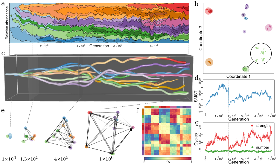
Figure 1: Evolutionary dynamics of a community driven by competitive interactions, with trade-off between fecundity and competitive abilities ($\delta=0.5$, $\lambda=300$, $\mu=0.001$, $m=0.02$, $N_{s}=10^{5}$). (a) Species’ frequencies over time (Muller plot): one color per species, vertical width of each colored region is relative abundance of respective species. Frequencies are recorded every $10^{4}$ generations over $10^{6}$ generations. (b) Distribution over trait space: Snapshot of distribution in trait space after $10^{6}$ generations, reduced to two dimensions that explain most of the variance in trait space (SM-4). Points and discs are strains and species, respectively. Magnified disc in lower right corner shows strains in the light green species disc. Disc diameter scales with abundance of species. This snapshot consists of 660 strains in 10 species. (c) Evolutionary dynamics in trait space: Snapshots as in panel (b), but concatenated for all times (horizontal axis), from the monomorphic first generation to $10^{6}$ generations. (d) Functional diversity over time in terms of the size of minimum spanning tree (SMST) in trait space (SM-6). At $1.75\times 10^{6}$ generations an evolutionary collapse happens in which all species but one go extinct (vertical dashed line). (e) Evolution of interaction network: several snapshots from panel (c) with interactions between species (colored discs) as directed edges. Directions and strengths of edges given by signs and absolute values, respectively, of averages over $\bm{I}_{\alpha\beta}-\bm{I}_{\beta\alpha}$, with $\alpha,\beta$ the component strains of the species linked by edge. (f) Heatmap of interaction matrix $\mathbf{I}$ for generation $10^{6}$. Row and column order reflects species clusters, consistent with panel (b) and indicated by color bars along top and left. Colors inside heatmap represent interaction rates (color-key along bottom). (g) Numbers and average strengths of cycles over time in green and red, respectively. The strength of a cycle is defined by its weakest edge. Number and average strength given in units of number and average strength of equivalent random network, respectively (SM-7). Right ends in (a) and (c) correspond to panel (b) and (f). Colors of species are the same in panels (a), (b), (c), (e) and (f). Note that time scales differ between panels (a), (c) and (d), (g).

Impact of trade-off and lifespan on diversity

The eco-evolutionary dynamics described above depend on lifespan and trade-off between replication and competitive ability. To show this we study properties of interaction matrix and trait diversity. Fig. 2 relates average interaction rate $\left\langle I\right\rangle$ and average cycle strength $\rho$ to trade-off parameter $\delta$ at fixed lifespan $\lambda$. Fig. 2b summarizes the behavior of diversity as function of $\delta$ and $\lambda$. Overall, we see in this phase diagram a weak dependency on $\lambda$ and a strong impact of $\delta$, with four distinct phases (I-IV) from low to high $\delta$.

Without trade-off, strains do not have to sacrifice replication rate for better competitive abilities. We have a low-diversity population dominated by Darwinian demons, species with high competitive ability and replication rate. Quick predominance of such strategies impedes formation of a diverse network. Increasing $\delta$ in phase I ($\delta\lesssim 0.2$) slightly increases $\left\langle I\right\rangle$ and $\rho$ (Fig. 2a): biotic selection pressure exerted by inter-species interactions starts to generate diverse communities (left inset in Fig. 2b, SM-6). However, the weak trade-off still favors investing in higher competitive ability. When increasing $\delta$ further (phase II), trade-off starts to force strains to choose between higher replication rate $r$ or better competitive abilities $C$. Neither extreme generates viable species: sacrificing $r$ completely for maximum $C$ stalls species dynamics, whereas maximum $r$ leads to inferior $C$. Thus strains seek middle ground values in both $r$ and $C$. The nature of $C$ as mean of interactions (Eq. 2) allows for many combinations of interaction traits with approximately the same mean. Thus in a middle range of $r$ and $C$, many strategies with the same overall fitness are possible, which is a condition of diversity. From this multitude of strategies, sets of trait combinations emerge in which strains with different combinations keep each other in check, e.g. in the form of competitive rock-paper-scissors-like cycles between species described above. An equivalent interpretation is the emergence of diverse sets of non-overlapping compartments or trait space niches (Fig. 1b,f). Diversity in this phase II is the highest and most stable (middle inset in Fig. 2b, SM-6). As $\delta$ approaches $0.7$, $\left\langle I\right\rangle$ and $\rho$ plummet (Fig. 2a) to interaction rates comparable to noise level $m$, and a cycle strength typical for the neutral model (horizontal gray ribbon in Fig. 2a), respectively. The sharp drop of $\left\langle I\right\rangle$ and $\rho$ at $\delta\approx 0.7$ is reminiscent of a phase transition. As expected for a phase transition, the steepness increases with system size (SM-8). For $\delta\gtrsim 0.7$ interaction rates never grow and no structure emerges; diversity remains low and close to a neutral system. The sharp transition at $\delta\approx 0.7$ which is visible in practically all diversity measures (between phases II and III in Fig. 2b, SM-6) is a transition from a system dominated by biotic selection pressure to a neutral system. In high-trade-off phase III, any small change in $C$ changes $r$ drastically. For instance, given a strain $S$ with $r$ and $C$, a closely related mutant $S^{\prime}$ with $C^{\prime}\lessapprox C$ will have $r^{\prime}\gg r$ (because of the large trade-off), and therefore will invade $S$ quickly. Thus, diversity in phase III will remain stable and low, characterized by a group of similar strains with no effective interaction and hence no diversification to distinct species (right inset in Fig. 2b, SM-6).

In this high trade-off regime, lifespan comes into play: here, decreasing $\lambda$ can make lives too short for replication. These hostile conditions minimize diversity and favor extinction (phase IV).

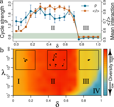
Figure 2: Effects of trade-off $\delta$ and lifespan $\lambda$ on community structure and diversity. (a) Average interaction rates $\left\langle I\right\rangle$ (orange squares) and average strength of cycles $\rho$ (blue circles) as function of $\delta$. Average cycle strength is given in units of average strength of random networks for the respective trade-off (SM-7). Averages are calculated over three different simulations, each over $5\times 10^{6}$generations with $\mu=0.001$, $m=0.02$, $\lambda=\infty$ and $N_{S}=10^{5}$. Error bars are standard deviations averaged over three concatenated simulations. The shaded area marks cycle strength for a neutral model with corresponding parameters $\pm$ standard deviation. (b) Phase diagram of diversity as function of $\delta$ and $\lambda$. Diversity is given as consensus of several quantities (SM-6). Four phases (I-IV) can be distinguished. Insets at the top margin are representative MDS plots (SM-4) of strain distributions in trait space, as in Fig. 1b, with $\lambda=10^{5}$ but different values of $\delta$ (left to right: I with $\delta=0.11$; II with $\delta=0.5$; III with $\delta=0.89$). Panel (a) corresponds to a horizontal cross-section through the phase diagram in panel (b) with $\lambda=\infty$ for $\left\langle I\right\rangle$ and $\rho$ as diversity measures.

Trade-off, resource availability, and diversity

There is a well-known but not well understood unimodal relationship between biomass productivity and diversity (“humpback curve”,Smith (2007); Vallina et al. (2014)): diversity culminates once at middle values of productivity. This behavior is reminiscent of horizontal sections through the phase diagram in Fig. 2b, though here the driving parameter is not productivity but trade-off. However, we can make the following argument for a monotonous relation between productivity and trade-off. First we note that biomass productivity is a function of available resources: the larger the available resources, the higher the productivity. This allows us to argue in terms of available resources. If then a species has a high replication rate in an environment with scarce resources, its individuals will not be very competitive since for each of the numerous offspring individuals there is little material or energy available. On the other hand, if a species under these resource-limited conditions has competitively constructed individuals it cannot produce many of them. This corresponds to a strong trade-off between replication and competitive ability for scarce resources. At the opposite, rich end of the resource scale, species are not confronted with such hard choices between replication rate and competitive ability, i.e. we have a weak trade-off. Taken together, the trade-off axis should roughly correspond to the inverted resource axis: strong trade-off for poor resources (or low productivity), weak trade-off for rich resources (or high productivity); a detailed analytical derivation will be presented elsewhere. The fact that ITEEM produces this humpback curve that is frequently observed in planktonic systems Vallina et al. (2014) proposes trade-off as underlying mechanism of this productivity-diversity relation.

Frequency-dependent selection

Observation of eco-evolutionary trajectories as in Fig. 1 suggested the hypothesis that speciation events in ITEEM simulations do not occur with a constant rate and independently of each other, but that one speciation makes a following speciation more likely. We therefore tested whether the distribution of time between speciation or extinction events is compatible with a constant rate Poisson process (SM-9). At long inter-event times we see the same decaying distribution for the Poisson process and for the ITEEM data. However, for shorter times there are significant deviations from a Poisson process for speciation and extinction events: at inter-event times of around $10\text{\textsuperscript{4}}$ the number of events decreases for a Poisson process but increases in ITEEM simulations. This confirms the above hypothesis that new species increase the probability for generation of further species, and additionally that loss of a species makes further losses more likely. This result is similar to the frequency-dependent selection observed in microbial systems where new species open new niches for further species, or the loss of species causes the loss of dependent species Herron and Doebeli (2013); Maddamsetti et al. (2015).

Effect of mutation rate on diversity

Simulations with different mutation rates ($\mu=10^{-4},5\times 10^{-4},10^{-3},5\times 10^{-3}$) show that in ITEEM diversity grows faster and to a higher level with increasing mutation rate, but without changing the overall structure of the phase diagram (SM-10). One interesting tendency is that for higher mutation rates, the lifespan becomes more important at the interface of regions III and IV (high trade-offs), leading to an expansion of region III at the expense of hostile region IV: long lifespans in combination with high mutation rate establish low but viable diversity at strong trade-offs.

Comparison of ITEEM with neutral model

The neutral model introduced in the Model section has no meaningful interaction traits, and consequently no meaningful competitive ability or trade-off with replication rate. Instead, it evolves solely by random drift in phenotype space. Similarly to ITEEM, the neutral model generates a clumpy structure in trait space (SM-11), though here the species clusters are much closer and thus the functional diversity much lower. This can be demonstrated quantitatively by the size of the minimum spanning tree of populations in trait space that are much smaller and much less dynamic for the neutral model than for ITEEM at moderate trade-off (SM-11). For high trade-offs (region III, Fig. 2b), diversity and number of strong cycles in ITEEM are comparable to the neutral model (Fig. 2a).

Interaction based eco-evolutionary models have received some attention in the past Ginzburg et al. (1988); Solé (2002); Tokita and Yasutomi (2003); Shtilerman et al. (2015) but then were almost forgotten, despite remarkable results. We think that these works have pointed to a possible solution of a hard problem: The complexity of evolving ecosystems is immense, and it is therefore difficult to find a representation suitable for the development of a statistical mechanics that enables qualitative and quantitative analysis Weber et al. (2017). Modeling in terms of interaction traits, rather than detailed descriptions of genotypes or phenotypes, then coarse-grains these complex systems in a natural, biologically meaningful way.

Despite these advantages, interaction based models so far have not shown some key features of real systems, e.g. emergence of large, stable and complex diversity, or mass extinctions with the subsequent recovery of diversity Tokita and Yasutomi (2003); Kärenlampi (2014). Therefore, interaction based models were supplemented by ad hoc features, such as special types of mutations Tokita and Yasutomi (2003), induced extinctions Vandewalle and Ausloos (1995), or enforcement of partially connected interaction graphs Kärenlampi (2014).

Trade-off between replication and competitive ability have now been experimentally established as essential to living systems Stearns (1989); Agrawal et al. (2010). Our results with ITEEM show that trade-offs fundamentally impact eco-evolutionary dynamics, in agreement with other eco-evolutionary models with trade-off Huisman et al. (2001); Bonsall (2004); de Mazancourt and Dieckmann (2004); Beardmore et al. (2011). Remarkably, we observe with ITEEM sustained high diversity in a well-mixed homogeneous system, without violating the competitive exclusion principle. This is possible because moderate life-history trade-offs force evolving species to adopt different strategies or, in other words, lead to the emergence of well-separated niches in interaction space.

The current model has important limitations. For instance, the trade-off formulation was chosen to reflect reasonable properties in a minimalistic way, that should be revised or refined as more experimental data become available. Secondly, we have assumed a single, limiting resource in a well-mixed system to investigate the mechanisms behind diversification in competitive communities and possibility of niche differentiation without resource partitioning or geographic isolation. However, in nature, there will in general be several limiting resources and abiotic factors. It is possible to include those as additional rows and columns in the interaction matrix $\mathbf{I}$.

Despite its simplifications, ITEEM reproduces in a single framework several phenomena of eco-evolutionary dynamics that previously were addressed with a range of distinct models or not at all, namely sympatric and concurrent speciation with the emergence of new niches in the community, recovery after mass-extinctions, large and sustained functional diversity with hierarchical organization, and a unimodal diversity distribution as function of trade-off between replication and competition. The model allows detailed analysis of mechanisms and could guide experimental tests.