Online to Offline Conversions, Universality and Adaptive Minibatch Sizes

Abstract

We present an approach towards convex optimization that relies on a novel scheme which converts online adaptive algorithms into offline methods. In the offline optimization setting, our derived methods are shown to obtain favourable adaptive guarantees which depend on the harmonic sum of the queried gradients. We further show that our methods implicitly adapt to the objective’s structure: in the smooth case fast convergence rates are ensured without any prior knowledge of the smoothness parameter, while still maintaining guarantees in the non-smooth setting. Our approach has a natural extension to the stochastic setting, resulting in a lazy version of SGD (stochastic GD), where minibathces are chosen adaptively depending on the magnitude of the gradients. Thus providing a principled approach towards choosing minibatch sizes.

1 Introduction

Over the past years data adaptiveness has proven to be crucial to the success of learning algorithms. The objective function underlying “big data” applications often demonstrates intricate structure: the scale and smoothness are often unknown and may change substantially in between different regions/directions. Learning methods that acclimatize to these changes may exhibit superior performance compared to non adaptive procedures, which in turn might make the difference between success and failure in practice (see e.g. Duchi et al. (2011)).

State-of-the-art first order methods like AdaGrad, Duchi et al. (2011), and Adam, Kingma & Ba (2014), adapt the learning rate on the fly according to the feedback (i.e. gradients) received during the optimization process. AdaGrad and Adam are guaranteed to work well in the online convex optimization setting, where loss functions may be chosen adversarially and change between rounds. Nevertheless, this setting is harder than the stochastic/offline settings, which may better depict practical applications. Interestingly, even in the offline convex optimization setting it could be shown that in several scenarios very simple schemes may substantially outperform the output of AdaGrad/Adam. An example of such a simple scheme is choosing the point with the smallest gradient norm among all rounds. In the first part of this work we address this issue and design adaptive methods for the offline convex optimization setting. At heart of our derivations is a novel scheme which converts online adaptive algorithms into offline methods with favourable guarantees. Our shceme is inspired by standard online to batch conversions as introduced in the seminal work of Cesa-Bianchi, Conconi, and Gentile (2004).

A seemingly different issue is choosing the minibatch size, $b$, in the stochastic setting. Stochastic optimization algorithms that can access a noisy gradient oracle may choose to invoke the oracle $b$ times in every query point, subsequently employing an averaged gradient estimate. Theory for stochastic convex optimization suggests to use a minibatch of $b=1$, and predicts a degradation of $\sqrt{b}$ factor upon using larger minibatch sizes . Nevertheless in practice larger minibatch sizes are usually found to be effective. In the second part of this work we design stochastic optimization methods in which minibatch sizes are chosen adaptively without any theoretical degradation. These are natural extensions of the offline methods presented in the first part.

Our contributions:

Offline setting:

We present two (families of) algorithms AdaNGD (Alg. 2) and SC-AdaNGD (Alg. 3) for the convex/strongly-convex settings which achieve favourable adaptive guarantees (Thms. 2.1, 2.2, 3.1, 3.2 ). The latter theorems also establish their universality, i.e., their ability to implicitly take advantage of the objective’s smoothness and attain rates as fast as GD would have achieved if the smoothness parameter was known.
Concretely, without the knowledge of the smoothness parameter our algorithm ensures an $O(1/\sqrt{T})$ rate in general convex case and an $O(1/T)$ rate if the objective is also smooth (Thms. 2.1, 2.2). In the strongly-convex case our algorithm ensures an $O(1/T)$ rate in general and an $O(\exp(-\gamma T))$ rate if the objective is also smooth (Thm. 3.2 ), where $\gamma$ is the condition number.

Stochastic setting:

We present Lazy-SGD (Algorithm 4) which is an extension of our offline algorithms. Lazy-SGD employs larger minibatch sizes in points with smaller gradients, which selectively reduces the variance in the “more important” query points. Lazy-SGD guarantees are comparable with SGD in the convex/strongly-convex settings (Thms. 4.2, 4.3).

On the technical side, our online to offline conversion schemes employ three simultaneous mechanisms: an online adaptive algorithm used in conjunction with gradient normalization and with a respective importance weighting. To the best of our knowledge the combination of the above techniques is novel, and we believe it might also find use in other scenarios.

This paper is organized as follows. In Sections 2,3, we present our methods for the offline convex/strongly-convex settings. Section 4 describes our methods for the stochastic setting. In Section 5 we discuss several extensions, and Section 6 presents a preliminary experimental study. Section 7 concludes.

1.1 Related Work

Duchi, Hazan, and Singer (2011), simultaneously to McMahan & Streeter (2010), were the first to suggest AdaGrad—an adaptive gradient based method, and prove its efficiency in tackling online convex problems. AdaGrad was subsequently adjusted to the deep-learning setting to yield the RMSprop, Tieleman & Hinton (2012), and Adadelta, Zeiler (2012), heuristics. Kingma & Ba (2014), combined ideas from AdaGrad together with momentum machinery, Nesterov (1983), and devised Adam—a popular adaptive algorithm which is often the method of choice in deep-learning applications.

An optimization procedure is called universal if it implicitly adapts to the objective’s smoothness. In Nesterov (2015), universal gradient methods are devised for the general convex setting. Concretely, without the knowledge of the smoothness parameter, these methods attain the standard $O(1/T)$ and accelerated $O(1/T^{2})$ rates for smooth objectives, and an $O(1/\sqrt{T})$ rate in the non-smooth case. The core technique in this work is a line search procedure which estimates the smoothness parameter in every iteration. For strongly-convex and smooth objectives, line search techniques,Wright & Nocedal (1999), ensure linear convergence rate, without the knowledge of the smoothness parameter. However, line search is not “fully universal”, in the sense that it holds no guarantees in the non-smooth case. For the latter setting we present a method which “fully universal” (Thm. 3.2), nevertheless it requires the strong-convexity parameter. Composite optimization methods, Nesterov (2013), may obtain fast rates even for non-smooth objectives. Nevertheless, proximal-GD may separately access the gradients of the ”smooth part” of the objective, which is a more refined notion than the normal oracle access to the (sub-)gradient of the whole objective.

The usefulness of employing normalized gradients was demonstrated in several non-convex scenarios. In the context of quasi-convex optimization, Nesterov (1984), and Hazan et al. (2015), established convergence guarantees for the offline/stochastic settings. More recently, it was shown in Levy (2016), that normalized gradient descent is more appropriate than GD for saddle-evasion scenarios.

In the context of stochastic optimization, the effect of minibatch size was extensively investigated throughout the past years, Dekel et al. (2012); Cotter et al. (2011); Shalev-Shwartz & Zhang (2013); Li et al. (2014); Takáč et al. (2015); Jain et al. (2016). Yet, all of these studies: (i) assume a smooth expected loss, (ii) discuss fixed minibatch sizes. Conversely, our work discusses adaptive minibatch sizes, and applies to both smooth/non-smooth expected losses.

1.2 Preliminaries

Notation:

$\|\cdot\|$ denotes the $\ell_{2}$ norm, $G$ denotes a bound on the norm of the objective’s gradients, and $[T]:=\{1,\ldots,T\}$. For a set $\mathcal{K}\in{\mathbb{R}}^{d}$ its diameter is defined as $D=\sup_{x,y\in\mathcal{K}}\|x-y\|$. Next we define $H$-strongly-convex/$\beta$-smooth functions,

$$f(y)\geq f(x)+\nabla f(x)^{\top}(y-x)+\frac{H}{2}\|x-y\|^{2};\quad\forall x,y\in\mathcal{K}\quad\textbf{($H$-strong-convexity)}$$

$$f(y)\leq f(x)+\nabla f(x)^{\top}(y-x)+\frac{\beta}{2}\|x-y\|^{2};\quad\forall x,y\in\mathcal{K}\quad\textbf{($\beta$-smoothness)}$$

1.2.1 AdaGrad

Algorithm 1 Adaptive Gradient Descent (AdaGrad)

  Input: #Iterations $T$, $x_{1}\in{\mathbb{R}}^{d}$, set $\mathcal{K}$

  Set: $Q_{0}=0$

  for $t=1\ldots T$  do

     Calculate: $g_{t}=\nabla f_{t}(x_{t})$

     Update:

$$Q_{t}=Q_{t-1}+\|g_{t}\|^{2}$$

     Set $\eta_{t}=D/\sqrt{2Q_{t}}$

     Update:

$$x_{t+1}=\Pi_{\mathcal{K}}\left(x_{t}-\eta_{t}{g}_{t}\right)$$

  end for

The adaptive methods presented in this paper lean on AdaGrad (Alg. 1), a well known online optimization method which employs an adaptive learning rate. The following theorem states AdaGrad’s guarantees, Duchi et al. (2011),

Theorem 1.1.

Let $\mathcal{K}$ be a convex set with diameter $D$. Let $\{f_{t}\}_{t=1}^{T}$ be an arbitrary sequence of convex loss functions. Then Algorithm 1 guarantees the following regret;

$$\sum_{t=1}^{T}f_{t}(x_{t})-\min_{x\in\mathcal{K}}\sum_{t=1}^{T}f_{t}(x)~{}\leq~{}\sqrt{2D^{2}\sum_{t=1}^{T}\|g_{t}\|^{2}}~{}.$$

2 Adaptive Normalized Gradient Descent (AdaNGD)

In this section we discuss the convex optimization setting and introduce our $\text{AdaNGD}_{k}$ algorithm. We first derive a general convergence rate which holds for any $k\in{\mathbb{R}}$. Subsequently, we elaborate on the $k=1,2$ cases which exhibit universality as well as adaptive guarantees that may be substantially better compared to standard methods.

Our method $\text{AdaNGD}_{k}$ is depicted in Alg. 2. This algorithm can be thought of as an online to offline conversion scheme which utilizes AdaGrad (Alg. 1) as a black box and eventually outputs a weighted sum of the online queries. Indeed, for a fixed $k\in{\mathbb{R}}$, it is not hard to notice that $\text{AdaNGD}_{k}$ is equivalent to invoking AdaGrad with the following loss sequence $\{\tilde{f}_{t}(x):={g_{t}^{\top}x}/{\|g_{t}\|^{k}}\}_{t=1}^{T}$. And eventually weighting each query point inversely proportional to the $k$’th power norm of its gradient. The reason behind this scheme is that in offline optimization it makes sense to dramatically reduce the learning rate upon uncountering a point with a very small gradient. For $k\geq 1$, this is achieved by invoking AdaGrad with gradients normalized by their $k$’th power norm. Since we discuss constrained optimization, we use the projection operator defined as,

$$\Pi_{\mathcal{K}}(y):=\min_{x\in\mathcal{K}}\|x-y\|~{}.$$

Algorithm 2 Adaptive Normalized Gradient Descent ($\text{AdaNGD}_{k}$)

  Input: #Iterations $T$, $x_{1}\in{\mathbb{R}}^{d}$, set $\mathcal{K}$ , parameter $k$

  Set: $Q_{0}=0$

  for $t=1\ldots T-1$  do

     Calculate: $g_{t}=\nabla f(x_{t}),\;\hat{g}_{t}={g_{t}}/{\|g_{t}\|^{k}}$

     Update:

$$Q_{t}=Q_{t-1}+{1}/{\|g_{t}\|^{2(k-1)}}$$

     Set $\eta_{t}=D/\sqrt{2Q_{t}}$

     Update:

$$x_{t+1}=\Pi_{\mathcal{K}}\left(x_{t}-\eta_{t}\hat{g}_{t}\right)$$

  end for

  Return: $\bar{x}_{T}=\sum_{t=1}^{T}\frac{1/\|g_{t}\|^{k}}{\sum_{\tau=1}^{T}1/\|g_{\tau}\|^{k}}x_{t}$

The following lemma states the guarantee of AdaNGD for a general $k$:

Lemma 2.1.

Let $k\in{\mathbb{R}}$, $\mathcal{K}$ be a convex set with diameter $D$, and $f$ be a convex function; Also let $\bar{x}_{T}$ be the output of $\text{AdaNGD}_{k}$ (Algorithm 2), then the following holds:

$$f(\bar{x}_{T})-\min_{x\in\mathcal{K}}f(x)~{}\leq~{}\frac{\sqrt{2D^{2}\sum_{t=1}^{T}1/\|g_{t}\|^{2(k-1)}}}{\sum_{t=1}^{T}1/\|g_{t}\|^{k}}$$

Proof sketch.

Notice that the $\text{AdaNGD}_{k}$ algorithm is equivalent to applying AdaGrad to the following loss sequence: $\{\tilde{f}_{t}(x):={g_{t}^{\top}x}/{\|g_{t}\|^{k}}\}_{t=1}^{T}$. Thus, applying Theorem 1.1, and using the definition of $\bar{x}_{T}$ together with Jensen’s inequality the lemma follows. ∎

For $k=0$, Algorithm 2 becomes AdaGrad (Alg. 1). Next we focus on the cases where $k=1,2$, showing improved adaptive rates and universality compared to GD/AdaGrad. These improved rates are attained thanks to the adaptivity of the learning rate: when query points with small gradients are encountered, $\text{AdaNGD}_{k}$ (with $k\geq 1$) reduces the learning rate, thus focusing on the region around these points. The hindsight weighting further emphasizes points with smaller gradients.

2.1 $\text{AdaNGD}_{1}$

Here we show that $\text{AdaNGD}_{1}$ enjoys a rate of $O(1/\sqrt{T})$ in the non-smooth convex setting, and a fast rate of $O(1/T)$ in the smooth setting. We emphasize that the same algorithm enjoys these rates simultaneously, without any prior knowledge of the smoothness or of the gradient norms.

From Algorithm 2 it can be noted that for $k=1$ the learning rate becomes independent of the gradients, i.e. $\eta_{t}=D/\sqrt{2t}$, the update is made according to the direction of the gradients, and the weighting is inversely proportional to the norm of the gradients. The following Theorem establishes the guarantees of $\text{AdaNGD}_{1}$ (see proof in Appendix A.3),

Theorem 2.1.

Let $k=1$, $\mathcal{K}$ be a convex set with diameter $D$, and $f$ be a convex function; Also let $\bar{x}_{T}$ be the outputs of $\text{AdaNGD}_{1}$ (Alg. 2), then the following holds:

$$f(\bar{x}_{T})-\min_{x\in\mathcal{K}}f(x)~{}\leq~{}\frac{\sqrt{2D^{2}T}}{\sum_{t=1}^{T}1/\|g_{t}\|}~{}\leq~{}\frac{\sqrt{2}GD}{\sqrt{T}}~{}.$$

Moreover, if $f$ is also $\beta$-smooth and the global minimum $x^{*}=\arg\min_{x\in{\mathbb{R}}^{n}}f(x)$ belongs to $\mathcal{K}$, then:

$$f(\bar{x}_{T})-\min_{x\in\mathcal{K}}f(x)~{}\leq~{}\frac{D\sqrt{T}}{\sum_{t=1}^{T}1/\|g_{t}\|}~{}\leq~{}\frac{4\beta D^{2}}{T}~{}.$$

Proof sketch.

The data dependent bound is a direct corollary of Lemma 2.1. The general case bound holds directly by using $\|g_{t}\|\leq G$. The bound for the smooth case is proven by showing $\sum_{t=1}^{T}\|g_{t}\|\leq O(\sqrt{T})$. This translates to a lower bound $\sum_{t=1}^{T}1/\|g_{t}\|\geq\Omega(T^{3/2})$, which concludes the proof. ∎

The data dependent bound in Theorem 2.1 may be substantially better compared to the bound of the GD/AdaGrad. As an example, assume that half of the gradients encountered during the run of the algorithm are of $O(1)$ norms, and the other gradient norms decay proportionally to $O(1/t)$. In this case the guarantee of GD/AdaGrad is $O(1/\sqrt{T})$, whereas $\text{AdaNGD}_{1}$ guarantees a bound that behaves like $O(1/T^{3/2})$. Note that the above example presumes that all algorithms encounter the same gradient magnitudes, which might be untrue. Nevertheless in the smooth case $\text{AdaNGD}_{1}$ provably benefits due to its adaptivity.

GD Vs $\text{AdaNGD}_{1}$ in the smooth case: In order to achieve the $O(1/T)$ rate for smooth objectives GD employs a constant learning rate, $\eta_{t}=1/\beta$. It is worth to compare this GD algorithm with $\text{AdaNGD}_{1}$ in the smooth case: For both methods the steps become smaller as the algorithm progresses. However, the mechanism is different: in GD the learning rate is constant, but the gradient norms decay; while in $\text{AdaNGD}_{1}$ the learning rate is decaying, but the norm of the normalized gradients is constant.

2.2 $\text{AdaNGD}_{2}$

Here we show that $\text{AdaNGD}_{2}$ enjoys comparable guarantees to $\text{AdaNGD}_{1}$ in the general/smooth case. Similarly to $\text{AdaNGD}_{1}$ the same algorithm enjoys these rates simultaneously, without any prior knowledge of the smoothness or of the gradient norms. The following Theorem establishes the guarantees of $\text{AdaNGD}_{2}$ (see proof in Appendix A.4),

Theorem 2.2.

Let $k=2$, $\mathcal{K}$ be a convex set with diameter $D$, and $f$ be a convex function; Also let $\bar{x}_{T}$ be the outputs of $\text{AdaNGD}_{2}$ (Alg. 2), then the following holds:

$$f(\bar{x}_{T})-\min_{x\in\mathcal{K}}f(x)\leq\frac{\sqrt{2D^{2}}}{\sqrt{\sum_{t=1}^{T}1/\|g_{t}\|^{2}}}~{}\leq~{}\frac{\sqrt{2}GD}{\sqrt{T}}~{}.$$

Moreover, if $f$ is also $\beta$-smooth and the global minimum $x^{*}=\arg\min_{x\in{\mathbb{R}}^{n}}f(x)$ belongs to $\mathcal{K}$, then:

$$f(\bar{x}_{T})-\min_{x\in\mathcal{K}}f(x)~{}\leq~{}\frac{\sqrt{2D^{2}}}{\sqrt{\sum_{t=1}^{T}1/\|g_{t}\|^{2}}}~{}\leq~{}\frac{4\beta D^{2}}{T}~{}.$$

Proof sketch.

The data dependent bound is a direct corollary of Lemma 2.1. The general case bound holds directly by using $\|g_{t}\|\leq G$. The bound for the smooth case is proven by showing $\sum_{t=1}^{T}1/\|g_{t}\|^{2}\geq\Omega(T^{2})$, which concludes the proof. ∎

It is interesting to note that $\text{AdaNGD}_{2}$ will have always performed better than AdaGrad, had both algorithms encountered the same gradient norms. This is due to the well known inequality between arithmetic and harmonic means, Bullen et al. (2013),

$$\frac{1}{T}\sum_{t=1}^{T}a_{t}\geq\frac{1}{\frac{1}{T}\sum_{t=1}^{T}1/a_{t}},\qquad\forall\{a_{t}\}_{t=1}^{T}\subset{\mathbb{R}}_{+}~{},$$

which directly implies,

$$\frac{1}{\sqrt{\sum_{t=1}^{T}1/\|g_{t}\|^{2}}}~{}\leq~{}\frac{1}{T}\sqrt{\sum_{t=1}^{T}\|g_{t}\|^{2}}~{}.$$

3 Adaptive NGD for Strongly Convex Functions

Here we discuss the offline optimization setting of strongly convex objectives. We introduce our $\text{SC-AdaNGD}_{k}$ algorithm, and present convergence rates for general $k\in{\mathbb{R}}$. Subsequently, we elaborate on the $k=1,2$ cases which exhibit universality as well as adaptive guarantees that may be substantially better compared to standard methods.

Algorithm 3 Strongly-Convex AdaNGD ($\text{SC-AdaNGD}_{k}$)

  Input: #Iterations $T$, $x_{1}\in{\mathbb{R}}^{d}$, set $\mathcal{K}$, strong-convexity $H$, parameter $k$

  Set: $Q_{0}=0$

  for $t=1\ldots T-1$  do

     Calculate: $g_{t}=\nabla f(x_{t}),\;\hat{g}_{t}={g_{t}}/{\|g_{t}\|^{k}}$

     Update:

$$Q_{t}=Q_{t-1}+{1}/{\|g_{t}\|^{k}}$$

     Set $\eta_{t}={1}/{HQ_{t}}$

     Update:

$$x_{t+1}=\Pi_{\mathcal{K}}\left(x_{t}-\eta_{t}\hat{g}_{t}\right)$$

  end for

  Return: $\bar{x}_{T}=\sum_{t=1}^{T}\frac{1/\|g_{t}\|^{k}}{\sum_{\tau=1}^{T}1/\|g_{\tau}\|^{k}}x_{t}$

Our $\text{SC-AdaNGD}_{k}$ algorithm is depicted in Algorithm 3. Similarly to its non strongly-convex counterpart, $\text{SC-AdaNGD}_{k}$ can be thought of as an online to offline conversion scheme which utilizes an online algorithm which we denote SC-AdaGrad The next Lemma states the guarantee of $\text{AdaNGD}_{k}$,

Lemma 3.1.

Let $k\in{\mathbb{R}}$, and $\mathcal{K}$ be a convex set. Let $f$ be an $H$-strongly-convex function; Also let $\bar{x}_{T}$ be the outputs of $\text{SC-AdaNGD}_{k}$ (Alg. 3), then the following holds:

$$f(\bar{x}_{T})-\min_{x\in\mathcal{K}}f(x)\leq\frac{1}{2H\sum_{t=1}^{T}\|g_{t}\|^{-k}}\sum_{t=1}^{T}\frac{\|g_{t}\|^{-2(k-1)}}{\sum_{\tau=1}^{t}\|g_{\tau}\|^{-k}}~{}.$$

Proof sketch.

In Appendix B.1 we present and analyze SC-AdaGrad. This is an online first order algorithm for strongly-convex functions in which the learning rate decays according to $\eta_{t}=1/\sum_{\tau=1}^{t}H_{\tau}$, where $H_{\tau}$ is the strong-convexity parameter of the loss function at time $\tau$. Then we show that $\text{SC-AdaNGD}_{k}$ is equivalent to applying SC-AdaGrad to the following loss sequence:

$$\left\{\tilde{f}_{t}(x)=\frac{1}{\|g_{t}\|^{k}}g_{t}^{\top}x+\frac{H}{2\|g_{t}\|^{k}}\|x-x_{t}\|^{2}\right\}_{t=1}^{T}~{}.$$

Applying the regret guarantees of SC-AdaGrad to the above sequence implies the following to hold for any $x\in\mathcal{K}$:

$$\sum_{t=1}^{T}\tilde{f}_{t}(x_{t})-\sum_{t=1}^{T}\tilde{f}_{t}(x)~{}\leq~{}\frac{1}{2H}\sum_{t=1}^{T}\frac{\|g_{t}\|^{-2(k-1)}}{\sum_{\tau=1}^{t}\|g_{\tau}\|^{-k}}~{}.$$ (1)

The lemma then follows by the the definition of $\bar{x}_{T}$ together with Jensen’s inequality. ∎

For $k=0$, SC-AdaNGD becomes the standard GD algorithm which uses learning rate of $\eta_{t}={1}/{Ht}$. Next we focus on the cases where $k=1,2$.

3.1 $\text{SC-AdaNGD}_{1}$

Here we show that $\text{SC-AdaNGD}_{1}$ enjoys an $\tilde{O}(1/T)$ rate for strongly-convex convex objectives, and a faster rate of $\tilde{O}(1/T^{2})$ assuming that the objective is also smooth. We emphasize that the same algorithm enjoys these rates simultaneously, without any prior knowledge of the smoothness or of the gradient norms. The following theorem establishes the guarantees of $\text{SC-AdaNGD}_{1}$ (see proof in Appendix B.2), ,

Theorem 3.1.

Let $k=1$, and $\mathcal{K}$ be a convex set. Let $f$ be a $G$-Lipschitz and $H$-strongly-convex function; Also let $\bar{x}_{T}$ be the outputs of $\text{SC-AdaNGD}_{1}$ (Alg. 3), then the following holds:

$$f(\bar{x}_{T})-\min_{x\in\mathcal{K}}f(x) ~{}\leq~{}\frac{G\left(1+\log\left(\sum_{t=1}^{T}\frac{G}{\|g_{t}\|}\right)\right)}{2H\sum_{t=1}^{T}\frac{1}{\|g_{t}\|}}$$

$$~{}\leq~{}\frac{G^{2}(1+\log T)}{2HT}~{}.$$

Moreover, if $f$ is also $\beta$-smooth and the global minimum $x^{*}=\arg\min_{x\in{\mathbb{R}}^{n}}f(x)$ belongs to $\mathcal{K}$, then,

$$f(\bar{x}_{T})-\min_{x\in\mathcal{K}}f(x) ~{}\leq~{}\frac{(\beta/H)G^{2}\left(1+\log T\right)^{2}}{HT^{2}}~{}.$$

3.2 $\text{SC-AdaNGD}_{2}$

Here we show that $\text{SC-AdaNGD}_{2}$ enjoys an $\tilde{O}(1/T)$ rate for strongly-convex convex objectives, and a faster rate of $\tilde{O}(\exp(-\gamma T))$ assuming that the objective is also smooth. We emphasize that the same algorithm enjoys these rates simultaneously, without any prior knowledge of the smoothness or of the gradient norms. In the case where $k=2$ the guarantee of SC-AdaNGD is as follows (see proof in Appendix B.3), ,

Theorem 3.2.

Let $k=2$, $\mathcal{K}$ be a convex set, and $f$ be a $G$-Lipschitz and $H$-strongly-convex function; Also let $\bar{x}_{T}$ be the outputs of $\text{SC-AdaNGD}_{2}$ (Alg. 3), then the following holds:

$$f(\bar{x}_{T})-\min_{x\in\mathcal{K}}f(x) ~{}\leq~{}\frac{1+\log(G^{2}\sum_{t=1}^{T}\|g_{t}\|^{-2})}{2H\sum_{t=1}^{T}\|g_{t}\|^{-2}}$$

$$~{}\leq~{}\frac{G^{2}(1+\log T)}{2HT}~{}.$$

Moreover, if $f$ is also $\beta$-smooth and the global minimum $x^{*}=\arg\min_{x\in{\mathbb{R}}^{n}}f(x)$ belongs to $\mathcal{K}$, then,

$$f(\bar{x}_{T})-\min_{x\in\mathcal{K}}f(x) ~{}\leq~{}\frac{3G^{2}}{2H}e^{-\frac{H}{\beta}T}\left(1+\frac{H}{\beta}T\right)~{}.$$

Intuition: Recall that for strongly-convex objectives the appropriate GD algorithm utilizes two very extreme learning rates for the general/smooth settings. While for the first setting the learning rate is decaying, $\eta_{t}\propto 1/t$, for the smooth case it is constant, $\eta_{t}=1/\beta$. A possible explanation to the universality of $\text{SCAdaNGD}_{2}$ is that it implicitly interpolate between these rates. Indeed the update rule of our algorithm can be written as follows,

$$x_{t+1}=x_{t}-\frac{1}{H}\frac{\|g_{t}\|^{-2}}{\sum_{\tau=1}^{t}\|g_{\tau}\|^{-2}}g_{t}~{}.$$

Thus, ignoring the hindsight weighting, $\text{SCAdaNGD}_{2}$ is equivalent to GD with an adaptive learning rate $\tilde{\eta}_{t}:={\|g_{t}\|^{-2}}/{H\sum_{\tau=1}^{t}\|g_{\tau}\|^{-2}}$. Now, when all gradient norms are of the same magnitude, then $\tilde{\eta}_{t}\propto 1/t$, which boils down to the standard GD for strongly-convex objectives. On the other hand, assume that the gradients are exponentially decaying, i.e., that $\|g_{t}\|\propto q^{t}$ for some $q<1$. In this case $\tilde{\eta}_{t}$ is approximately constant. We believe that the latter applies for strongly-convex and smooth objectives. Nevertheless, note that this intuition is still unsatisfactory since it applies to any $k>0$ and does not explain why $k=2$ is unique (and maybe this is not the case).

4 Adaptive NGD for Stochastic Optimization

Here we show that using data-dependent minibatch sizes, we can adapt our (SC-)$\text{AdaNGD}_{2}$ algorithms (Algs. 2, 3 with $k=2$) to the stochastic setting, and achieve the well know convergence rates for the convex/strongly-convex settings. Next we introduce the stochastic optimization setting, and then we present and discuss our Lazy SGD algorithm.

Setup:

We consider the problem of minimizing a convex/strongly-convex function $f:\mathcal{K}\mapsto{\mathbb{R}}$, where $\mathcal{K}\in{\mathbb{R}}^{d}$ is a convex set. We assume that optimization lasts for $T$ rounds; on each round $t=1,\ldots,T$, we may query a point $x_{t}\in\mathcal{K}$, and receive a feedback. After the last round, we choose $\bar{x}_{T}\in\mathcal{K}$, and our performance measure is the expected excess loss, defined as,

$$\mbox{\bf E}[f(\bar{x}_{T})]-\min_{x\in\mathcal{K}}f(x)~{}.$$

Here we assume that our feedback is a first order noisy oracle $\mathcal{G}:\mathcal{K}\mapsto{\mathbb{R}}^{d}$ such that upon querying $\mathcal{G}$ with a point $x_{t}\in\mathcal{K}$, we receive a bounded and unbiased gradient estimate, $\mathcal{G}(x_{t})$, such $\mbox{\bf E}[\mathcal{G}(x_{t})|x_{t}]=\nabla f(x_{t})$; $\|\mathcal{G}(x_{t})\|\leq G$. We also assume that the that the internal coin tosses (randomizations) of the oracle are independent. It is well known that variants of Stochastic Gradient Descent (SGD) are ensured to output an estimate $\bar{x}_{T}$ such that the excess loss is bounded by $O(1/\sqrt{T})/O(1/T)$ for the setups of convex/strongly-convex stochastic optimization, Nemirovskii et al. (1983), Hazan et al. (2007).

Notation: In this section we make a clear distinction between the number of queries to the gradient oracle, denoted henceforth by $T$; and between the number of iterations in the algorithm, denoted henceforth by $S$. We care about the dependence of the excess loss in $T$.

Algorithm 4 Lazy Stochastic Gradient Descent (LazySGD)

  Input: #Oracle Queries $T$, $x_{1}\in{\mathbb{R}}^{d}$, set $\mathcal{K}$, $\eta_{0}$, $p$

  Set: $t=0,\;s=0$

  while $t\leq T$  do

     Update: $s=s+1$

     Set $\mathcal{G}=\text{GradOracle}(x_{s})$, i.e., $\mathcal{G}$ generates i.i.d. noisy samples of $\nabla f(x_{s})$

     Get: $(\tilde{g}_{s},n_{s})=\text{AE}(\mathcal{G},T-t)$ % Adaptive Minibatch

     Update: $t=t+n_{s}$

     Calculate: $\hat{g}_{s}=n_{s}\tilde{g}_{s}$

     Set: $\eta_{s}=\eta_{0}/t^{p}$

     Update: $x_{s+1}=\Pi_{\mathcal{K}}\left(x_{s}-\eta_{s}\hat{g}_{s}\right)$

  end while

  Return: $\bar{x}_{T}=\sum_{i=1}^{s}\frac{n_{i}}{T}x_{i}~{}.$ (Note that $\sum_{i=1}^{s}n_{i}=T$)

Algorithm 5 Adaptive Estimate (AE)

  Input: random vectors generator $\mathcal{G}$, sample budget $T_{\max}$, sample factor $m_{0}$

  Set: $i=0,N=0$, $\tilde{g}_{0}=0$

  while  $N<T_{\max}$  do

     Take $\tau_{i}=\min\{2^{i},T_{\max}-N\}$ samples from $\mathcal{G}$

     Set $N\leftarrow N+\tau_{i}$

     Update:

$$\tilde{g}_{N}\leftarrow\text{Average of N samples received so far from }\mathcal{G}$$

     If $\|\tilde{g}_{N}\|>3m_{0}/\sqrt{N}$ then return $(\tilde{g}_{N},N)$

     Update $i\leftarrow i+1$

  end while

  Return: $(\tilde{g}_{N},N)$

4.1 Lazy Stochastic Gradient Descent

Data Dependent Minibatch sizes: The Lazy SGD (Alg. 4) algorithm that we present in this section, uses a minibatch size that changes in between query points. Given a query point $x_{s}$, Lazy SGD invokes the noisy gradient oracle $\tilde{O}(1/\|g_{s}\|^{2})$ times, where $g_{s}:=\nabla f(x_{s})$ . Thus, in contrast to SGD which utilizes a fixed number of oracle calls per query point, our algorithm tends to stall in points with smaller gradients, hence the name Lazy SGD.

Here we give some intuition regarding our adaptive minibatch size rule: Consider the stochastic optimization setting. However, imagine that instead of the noisy gradient oracle $\mathcal{G}$, we may access an improved (imaginary) oracle which provides us with unbiased estimates, $\tilde{g}(x)$, that are accurate up to some multiplicative factor, e.g.,

$$\mbox{\bf E}[\tilde{g}(x)]=\nabla f(x),\;\text{and }\frac{1}{2}\|\nabla f(x)\|\leq\|\tilde{g}(x)\|\leq 2\|\nabla f(x)\|~{}.$$

Then intuitively we could have used these estimates instead of the exact normalized gradients inside our (SC-)$\text{AdaNGD}_{2}$ algorithms (Algs. 2, 3 with $k=2$), and still get similar (in expectation) data dependent bounds. Quite nicely, we may use our original noisy oracle $\mathcal{G}$ to generate estimates from this imaginary oracle. This can be done by invoking $\mathcal{G}$ for $\tilde{O}(1/\|g_{s}\|^{2})$ times at each query point. Using this minibatch rule, the total number of calls to $\mathcal{G}$ (along all iterations) is equal to $T=\sum_{s=1}^{S}1/\|g_{s}\|^{2}$. Plugging this into the data dependent bounds of $\text{(SC-)AdaNGD}_{2}$ (Thms. 2.2, 3.2), we get the well known $\tilde{O}(1/\sqrt{T})$/$\tilde{O}(1/T)$ rates for the stochastic convex settings.

The imaginary oracle:

The construction of the imaginary oracle from the original oracle appears in Algorithm 5 (AE procedure) . It receives as an input, $\mathcal{G}$, a generator of independent random vectors with an (unknown) expected value $g\in{\mathbb{R}}^{d}$. The algorithm outputs two variables: $N$ which is an estimate of $1/\|g\|^{2}$, and $\tilde{g}_{N}$ an average of $N$ random vectors from $\mathcal{G}$. Thus, it is natural to think of $N\tilde{g}_{N}$ as an estimate for $g/\|g\|^{2}$. Moreover, it can be shown that $E[N(\tilde{g}_{N}-g)]=0$. Thus in a sense we receive an unbiased estimate. The guarantees of Algorithm 5 appear in the following lemma (see proof in Appendix C.1),

Lemma 4.1 (Informal).

Let $T_{\max}\geq 1,\delta\in(0,1)$. Suppose an oracle $\mathcal{G}:\mathcal{K}\mapsto{\mathbb{R}}^{d}$ that generates $G$-bounded i.i.d. random vectors with an (unknown) expected value $g\in{\mathbb{R}}^{d}$. Then w.p.$\geq 1-\delta$, invoking AE (Algorithm 5), with $m_{0}=\Theta(G\log(1/\delta))$, it is ensured that:

$$N=\Theta(\min\{m_{0}/\|g\|^{2},T_{\max}\}),\;\text{and }\;E[N(\tilde{g}_{N}-g)]=0~{}.$$

Lazy SGD:

Now, plugging the output of the AE algorithm into our offline algorithms $\text{(SC-)AdaNGD}_{2}$, we get their stochastic variants which appears in Algorithm 4 (Lazy SGD). This algorithm is equivalent to the offline version of $\text{(SC-)AdaNGD}_{2}$, with the difference that we use $n_{s}$ instead of $1/\|\nabla f(x_{s})\|^{2}$ and $n_{s}\tilde{g}_{s}$ instead of $\nabla f(x_{s})/\|\nabla f(x_{s})\|^{2}$.

Let $T$ be a bound on the total number of queries to the the first order oracle $\mathcal{G}$, and $\delta$ be the confidence parameter used to set $m_{0}$ in the AE procedure. The next lemmas present the guarantees of LazySGD for the stochastic settings (see proofs in Appendix C.2, and C.3),

Lemma 4.2.

Let $\delta=O(1/T^{3/2})$, also let $\mathcal{K}$ be a convex set with diameter $D$, and $f$ be a convex function; and assume that $\|\mathcal{G}(x)\|\leq G$ w.p.$1$. Then using LazySGD (Algorithm 4) with $\eta_{0}=D/\sqrt{2}G$, $p=1/2$, ensures that:

$$\mbox{\bf E}[f(\bar{x}_{T})]-\min_{x\in\mathcal{K}}f(x)~{}\leq~{}O\left(\frac{GD\log(T)}{\sqrt{T}}\right)~{}.$$

Lemma 4.3.

Let $\delta=O(1/T^{2})$, also let $\mathcal{K}$ be a convex set, and $f$ be an $H$-strongly-convex convex function; and assume that $\|\mathcal{G}(x)\|\leq G$ w.p.$1$. Then using LazySGD (Algorithm 4) with $\eta_{0}=1/H$, $p=1$ ensures that:

$$\mbox{\bf E}[f(\bar{x}_{T})]-\min_{x\in\mathcal{K}}f(x)~{}\leq~{}O\left(\frac{G^{2}\log^{2}(T)}{HT}\right)~{}.$$

Note that LazySGD uses minibatch sizes that are adapted to the magnitude of the gradients, and still maintains the optimal $O(1/\sqrt{T})/O(1/T)$ rates. In contrast using a fixed minibatch size $b$ for SGD might degrade the convergence rates, yielding $O(\sqrt{b}/\sqrt{T})/O(b/T)$ guarantees. This property of LazySGD may be beneficial when considering distributed computations (see e.g. Dekel et al. (2012)).

5 Extensions

Acceleration: The catalyst approach, Lin et al. (2015), enables to take any first order method that ensures linear convergence rates in the strongly-convex and smooth case and transform it into an accelerated method obtaining $O(\exp(-\sqrt{\gamma}T))$ rate in the strongly-convex and smooth case, and $O(1/T^{2})$ rate in the smooth case. In particular, this acceleration applies to our $\text{SC-AdaNGD}_{2}$ Algorithm. Unfortunately, the catalyst approach requires the smoothness parameter, and the resulting accelerated $\text{SC-AdaNGD}_{2}$ is no longer universal.

Other online adaptive schemes: The adaptive methods that we have presented so far lean on AdaGrad (Alg. 1). Nevertheless, we may base our methods on other online algorithms with adaptive regret guarantees, and obtain convergence rates of the form,

$$f(\bar{x}_{T})-\min_{x\in\mathcal{K}}f(x)~{}\leq~{}\frac{\mathcal{R}^{\mathcal{A}}\left(g_{1}/\|g_{1}\|^{k},\ldots,g_{T}/\|g_{T}\|^{k}\right)}{\sum_{t=1}^{T}\|g_{t}\|^{k}}~{},$$

where $\mathcal{R}^{\mathcal{A}}(\theta_{1},\ldots,\theta_{T})$ is the regret bound of algorithm $\mathcal{A}$ with respect to the linear loss sequence $\{\theta_{t}^{\top}x\}_{t=1}^{T}$. For example we can use the very popular version of AdaGrad, which employs a separate learning rate to different directions. Also noteworthy is the Multiplicative Weights (MW) online algorithm, which over the simplex ensures a regret bound of the form (see Hazan & Koren (2012), Clarkson et al. (2012)),

$$\mathcal{R}^{MW}~{}\leq~{}\sqrt{\sum_{t=1}^{T}\|g_{t}\|_{\infty}^{2}\log(d)}~{}.$$

Using $\text{AdaNGD}_{k}$ with the appropriate modifications: AdaGrad$\leftrightarrow$MW, and $\ell_{2}\leftrightarrow\ell_{\infty}$, yields similar adaptive guarantees as in Theorems 2.1, 2.2, with the difference that, $D\leftrightarrow\log d$, and $\ell_{2}\leftrightarrow\ell_{\infty}$.

6 Experiments

As a preliminary experimental investigation we compare our $\text{SC-AdaNGD}_{k}$ to GD accelerated-GD, and line-search for two strongly-convex objectives. Concretely, we compare the above methods for the following quadratic (smooth) minimization problem,

$$\min_{x\in{\mathbb{R}}^{d}}R(x)~{}:=~{}\frac{1}{2}\sum_{i=1}^{d}i\cdot x_{i}^{2}~{}.$$

,and also for the following non-smooth problem,

$$\min_{\|x\|\leq 1}F(x)~{}:=~{}\frac{1}{2}\sum_{i=1}^{d}i\cdot x_{i}^{2}+\|x\|_{1}~{}.$$

where $x_{i}$ is the $i$’th component of $x$, and $\|x\|_{1}$ is the $\ell_{1}$ norm. Note that both $R$ and $F$ are $1$-strongly-convex, however $R$ is $d$-smooth while $F$ is non-smooth. Also, for both $R$ and $F$ the unique global minimum is in $x=0$. We initialize all of the methods at the same random point, and take $d=100$.

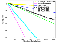
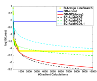
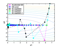
Figure 1: $\text{SC-AdaNGD}_{k}$ compared to GD, accelerated-GD and line-search. Left: strongly-convex and smooth objective, $R(\cdot)$. Middle: strongly-convex and non-smooth objective, $F(\cdot)$. Right: iterates of these methods for a 2D quadratic objective, $Z(\cdot)$.

The results are depicted in Fig. 1. In Fig. 1 we present our results for the smooth quadratic objective $R$. We compare three $\text{SC-AdaNGD}_{k}$ variants $k\in\{1,1.1,2\}$, to GD which uses a constant learning rate $\eta_{t}=1/\beta$ (recall $\beta=d=100$), and to Nesterov’s accelerated method. While this is not surprising that the latter demonstrates the best performance, it is surprising that all $\text{SC-AdaNGD}_{k}$ variants are performing better than GD/lines-search, and the $k=1.1$ variant substantially outperforms GD. Also, in contrast to GD, $\text{SC-AdaNGD}_{k}$ are not descent methods, in the sense that the losses are not necessarily monotonically decreasing from one iteration to another.

Fig. 1 shows the results for the non-smooth objective $F$, where we compare two $\text{SC-AdaNGD}_{k}$ variants $k\in\{1,2\}$, with two variants of GD, (i) const learning rate $\eta_{t}=1/\beta$, and (ii) decaying learning rate $\eta_{t}=1/Ht$. We have also compared to accelerated-GD and found its performance to be similar to GD-const (and therefore omitted). As can be seen, GD with a constant learning rate is doing very poorly, $\text{SC-AdaNGD}_{2}$ demonstrates the best performance, and GD-SC (decay) lags behind only by little. Note that for GD-SC (decay) we present results for a moving average over the GD iterates (which improve its performance).

The universality of $\text{SC-AdaNGD}_{k}$ for $k\in\{1,2\}$ is clearly evident from Figures 1 ,1. In order to learn more about the character of SC-AdaNGD, we have applied the above methods to a simple 2D quadratic objective,

$$Z(x)=x_{1}^{2}+10x_{2}^{2}~{}.$$

The progress (iterates) of these methods is presented in Fig. 1. It can be seen that GD and accelerated-GD converge quickly to the $x_{1}$ axis and progress along it towards $(0,0)$. Conversely, SC-AdaNGD methods progress diagonally, however take larger steps in the $x_{1}$ directions compared to GD and accelerated-GD.

Robustness: We have also examined the robustness of SC-AdaNGD compared to GD, accelerated-GD and line-search. We applied these methods to the quadratic objective $R$, however instead of the exact gradients we provided them with a slightly noisy and (unbiased) gradient feedback. The results when using noise perturbation magnitude of $10^{-6}$ appear in Fig. 2. This behaviour persisted when we employed other noise magnitudes.

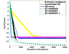
Figure 2: Robustness experiments comparing $\text{SC-AdaNGD}_{k}$ with GD and accelerated-GD for the strongly-convex and smooth objective, $R(\cdot)$. Gradient oracle is perturbed with $\propto 10^{-6}$ noise magnitude.

Stochastic setting: We made a few experiments in the stochastic setting. While examining LazySGD, we have found out that using the $n_{s}$ output of the AE procedure (Alg. 5) is a too crude estimate for $1/\|g_{s}\|^{2}$ (due to the doubling procedure), which lead to unsatisfactory performance. Instead, we found that using $1/\|\tilde{g}_{s}\|^{2}$ is a much better approximation, that works very well in practice.

An initial experimental study on several simple stochastic problems shows that LazySGD (with the above modification) compares with minibatch SGD, for various values of minibatch sizes. A more elaborate examination of LazySGD is left for future work.

7 Discussion

We have presented a new approach which exhibits universality and new adaptive bounds in the offline convex optimization setting, and provides a principled approach towards minibatch size selection in the stochastic setting.

Among the many questions that remain open is whether we can devise “accelerated” universal methods. Furthermore, our universality results only apply when the global minimum is inside the constraints. Thus, it is natural to seek for methods that ensure universality when this assumption is violated. Moreover, our algorithms depend on a parameter $k\in{\mathbb{R}}$, but only the cases where $k\in\{0,1,2\}$ are well understood. Investigating a wider spectrum of $k$ values is intriguing. Lastly, it is interesting to modify and test our methods in non-convex scenarios, especially in the context of deep-learning applications.

Appendix A Proofs for Section 2 (AdaNGD)

A.1 Proof of Theorem 1.1 (AdaGrad)

Proof.

Let $x\in\mathcal{K}$ and Consider the update rule $x_{t+1}=\Pi_{\mathcal{K}}(x_{t}-\eta_{t}g_{t})$. We can write:

$$\|x_{t+1}-x\|^{2}\leq\|x_{t}-x\|^{2}-2\eta_{t}g_{t}(x_{t}-x)+\eta_{t}^{2}\|g_{t}\|^{2}$$

Re-arranging the above we get:

$$g_{t}(x_{t}-x)\leq\frac{1}{2\eta_{t}}\left(\|x_{t}-x\|^{2}-\|x_{t+1}-x\|^{2}\right)+\frac{\eta_{t}}{2}\|g_{t}\|^{2}~{}.$$

Combined with the convexity of $f_{t}$ and summing over all rounds we conclude that $\forall x\in\mathcal{K}$,

$$\sum_{t=1}^{T}f_{t}(x_{t})-\sum_{t=1}^{T}f_{t}(x) \leq\sum_{t=1}^{T}\frac{\|x_{t}-x\|^{2}}{2}\left(\frac{1}{\eta_{t}}-\frac{1}{\eta_{t-1}}\right)+\sum_{t=1}^{T}\frac{\eta_{t}}{2}\|g_{t}\|^{2}$$

$$\leq\frac{D^{2}}{2}\sum_{t=1}^{T}\left(\frac{1}{\eta_{t}}-\frac{1}{\eta_{t-1}}\right)+\frac{D}{2\sqrt{2}}\sum_{t=1}^{T}\frac{\|g_{t}\|^{2}}{\sqrt{\sum_{\tau=1}^{t}\|g_{\tau}\|^{2}}}$$

$$\leq\frac{D}{2}\sqrt{2\sum_{t=1}^{T}\|g_{t}\|^{2}}+\frac{D}{\sqrt{2}}\sqrt{\sum_{t=1}^{T}\|g_{t}\|^{2}}$$

$$=\sqrt{2D^{2}\sum_{t=1}^{T}\|g_{t}\|^{2}}$$

here in the first inequality we denote $\eta_{0}=\infty$, the second inequality uses $\text{diam}\mathcal{K}=D$ and $\eta_{t}\leq\eta_{t-1}$, the third inequality uses the following lemma from McMahan & Streeter (2010):

Lemma A.1.

For any non-negative numbers $a_{1},\ldots,a_{n}$ the following holds:

$$\sum_{i=1}^{n}\frac{a_{i}}{\sqrt{\sum_{j=1}^{i}a_{j}}}\leq 2\sqrt{\sum_{i=1}^{n}a_{i}}$$

∎

A.2 Proof of Lemma 2.1

Proof.

Notice that $\text{AdaNGD}_{k}$ described in Algorithm 2, is equivalent to applying AdaGrad (Algorithm 1) to the following sequence of linear loss functions:

$$\left\{\tilde{f}_{t}(x):=\frac{1}{\|g_{t}\|^{k}}g_{t}^{\top}x\right\}_{t=1}^{T}~{}.$$

The regret bound of AdaGrad appearing in Theorem 1.1 implies the following for any $x\in\mathcal{K}$:

$$\sum_{t=1}^{T}\frac{1}{\|g_{t}\|^{k}}g_{t}^{\top}(x_{t}-x)~{}\leq~{}\sqrt{2D^{2}\sum_{t=1}^{T}{1}/{\|g_{t}\|^{2(k-1)}}}~{}.$$ (2)

Using the above bound together with Jensen’s inequality, enables to bound the excess loss of $\text{AdaNGD}_{k}$:

$$f(\bar{x}_{T})-f(x^{*}) ~{}\leq~{}\sum_{t=1}^{T}\frac{\|g_{t}\|^{-k}}{\sum_{\tau=1}^{T}\|g_{\tau}\|^{-k}}\big{(}f(x_{t})-f(x^{*})\big{)}$$

$$~{}\leq~{}\sum_{t=1}^{T}\frac{\|g_{t}\|^{-k}}{\sum_{\tau=1}^{T}\|g_{\tau}\|^{-k}}g_{t}^{\top}(x_{t}-x^{*})$$

$$~{}=~{}\frac{1}{\sum_{\tau=1}^{T}\|g_{\tau}\|^{-k}}\sum_{t=1}^{T}\frac{1}{\|g_{t}\|^{k}}g_{t}^{\top}(x_{t}-x^{*})$$

$$~{}\leq~{}\frac{\sqrt{2D^{2}\sum_{t=1}^{T}{1}/{\|g_{t}\|^{2(k-1)}}}}{\sum_{\tau=1}^{T}{1}/{\|g_{\tau}\|^{k}}}~{},$$

where the second line uses the gradient inequality. ∎

A.3 Proof of Theorem 2.1

Proof.

The data dependent bound,

$$f(\bar{x}_{T})-f(x^{*}) ~{}\leq~{}\frac{\sqrt{2D^{2}T}}{\sum_{t=1}^{T}{1}/{\|g_{t}\|}}~{},$$ (3)

is a direct corollary of Lemma 2.1 with $k=1$. Note that the above bound holds for both smooth/non-smooth cases. The general case bound holds directly by using $\|g_{t}\|\leq G$.

Next we focus on the second part of the theorem regarding the smooth case. We will first require the following lemma regarding smooth objectives,

Lemma A.2.

Let $F:{\mathbb{R}}^{d}\mapsto{\mathbb{R}}$ be a $\beta$-smooth function, and let $x^{*}=\operatorname*{arg\,min}_{x\in{\mathbb{R}}^{d}}F(x)$, then,

$$\|\nabla F(x)\|^{2}~{}\leq~{}2\beta\left(F(x)-F(x^{*})\right),\quad\forall x\in{\mathbb{R}}^{d}~{}.$$

The above lemma enables to upper bound sum of gradient norms in the query points of $\text{AdaNGD}_{1}$,

$$\sum_{t=1}^{T}\|g_{t}\| ~{}=~{}\sum_{t=1}^{T}\frac{\|g_{t}\|^{2}}{\|g_{t}\|}$$

$$~{}\leq~{}\sum_{t=1}^{T}\frac{{2\beta}}{\|g_{t}\|}\big{(}f(x_{t})-f(x^{*})\big{)}$$

$$~{}\leq~{}\sum_{t=1}^{T}\frac{{2\beta}}{\|g_{t}\|}g_{t}^{\top}(x_{t}-x^{*})$$

$$~{}=~{}2\beta\sum_{t=1}^{T}\hat{g}_{t}^{\top}(x_{t}-x^{*})$$

$$~{}\leq~{}2\sqrt{2}\beta D\sqrt{T}~{},$$ (4)

where the last line follows by the regret guarantee of AdaGrad for the following sequence (see Equation (2)),

$$\left\{\tilde{f}_{t}(x):=\frac{1}{\|g_{t}\|}g_{t}^{\top}x\right\}_{t=1}^{T}~{}.$$

The second line is a consequence of Lemma A.2 regarding smooth objectives. Now utilizing the convexity of the function $H(z)=1/z$ for $z>0$, and applying Equation (A.3), we may bound the sum of inverse gradients:

$$\sum_{\tau=1}^{T}\frac{1}{\|g_{\tau}\|} ~{}=~{}T\frac{1}{T}\sum_{\tau=1}^{T}\frac{1}{\|g_{\tau}\|}~{}\geq~{}T\frac{1}{\frac{1}{T}\sum_{\tau=1}^{T}\|g_{\tau}\|}$$

$$~{}\geq~{}T\frac{1}{2\sqrt{2}\beta D/\sqrt{T}}~{}.$$

Rearranging the latter equation, and using Equation (3) concludes the proof,

$$f(\bar{x}_{T})-\min_{x\in\mathcal{K}}f(x)~{}\leq~{}\frac{D\sqrt{2T}}{\sum_{\tau=1}^{T}1/\|g_{\tau}\|}~{}\leq~{}\frac{4\beta D^{2}}{T}~{}.$$

∎

A.4 Proof of Theorem 2.2

Proof.

The data dependent bound,

$$f(\bar{x}_{T})-f(x^{*}) ~{}\leq~{}\frac{\sqrt{2D^{2}}}{\sqrt{\sum_{t=1}^{T}{1}/{\|g_{t}\|^{2}}}}~{},$$ (5)

is a direct corollary of Lemma 2.1 with $k=2$. Note that the above bound holds for both smooth/non-smooth cases. The general case bound holds directly by using $\|g_{t}\|\leq G$.

We will now focus on the second part of the theorem regarding the smooth case. Let us lower bound $\sum_{t=1}^{T}1/\|g_{t}\|^{2}$ for $\text{AdaNGD}_{2}$:

$$T ~{}=~{}\sum_{t=1}^{T}\frac{\|g_{t}\|^{2}}{\|g_{t}\|^{2}}$$

$$~{}\leq~{}\sum_{t=1}^{T}\frac{{2\beta}}{\|g_{t}\|^{2}}\big{(}f(x_{t})-f(x^{*})\big{)}$$

$$~{}\leq~{}\sum_{t=1}^{T}\frac{{2\beta}}{\|g_{t}\|^{2}}g_{t}^{\top}(x_{t}-x^{*})$$

$$~{}=~{}2\beta\sum_{t=1}^{T}\left(\tilde{f}_{t}(x_{t})-\tilde{f}_{t}(x^{*})\right)$$

$$~{}\leq~{}2\sqrt{2}\beta D\sqrt{\sum_{t=1}^{T}\frac{1}{\|g_{t}\|^{2}}}~{},$$ (6)

where the last line follows by the regret guarantee of AdaGrad for the following sequence (see Equation (2)),

$$\left\{\tilde{f}_{t}(x)=\frac{1}{\|g_{t}\|^{2}}g_{t}^{\top}x\right\}_{t=1}^{T}~{}.$$

The second line is a consequence of Lemma A.2. Combining Equation (A.4) together with Equation (5) concludes the proof. ∎

A.5 Proof of Lemma A.2

Proof.

The $\beta$ smoothness of $F$ means the following to hold $\forall x,u\in{\mathbb{R}}^{d}$,

$$F(x+u)\leq F(x)+\nabla F(x)^{\top}u+\frac{\beta}{2}\|u\|^{2}~{}.$$

Taking $u=-\frac{1}{\beta}\nabla F(x)$ we get,

$$F(x+u)~{}\leq~{}F(x)-\frac{1}{\beta}\|\nabla F(x)\|^{2}+\frac{1}{2\beta}\|\nabla F(x)\|^{2}~{}.$$

Thus:

$$\|\nabla F(x)\| ~{}\leq~{}\sqrt{2\beta\big{(}F(x)-F(x+u)\big{)}}$$

$$~{}\leq~{}\sqrt{2\beta\big{(}F(x)-F(x^{*})\big{)}}~{},$$

where in the last inequality we used $F(x^{*})\leq F(x+u)$ which holds since $x^{*}$ is the global minimum. ∎

Appendix B Proofs for Section 3 (SC-AdaNGD)

B.1 Proof of Lemma 3.1

Algorithm 6 Strongly-Convex Adaptive Gradient Descent (SC-AdaGrad)

  Input: #Iterations $T$, $x_{1}\in{\mathbb{R}}^{d}$, set $\mathcal{K}$

  Set: $Q_{0}=0$

  for $t=1\ldots T$  do

     Calculate: $g_{t}=\nabla f_{t}(x_{t})$

     Let: $H_{t}$ be the strong-convexity parameter of $f_{t}(\cdot)$

     Update:

$$Q_{t}=Q_{t-1}+H_{t}$$

     Set $\eta_{t}=1/Q_{t}$

     Update:

$$x_{t+1}=\Pi_{\mathcal{K}}\left(x_{t}-\eta_{t}{g}_{t}\right)$$

  end for

Proof.

We will require the following extension of Theorem $1$ from Hazan et al. (2007). Its proof is provided in Section B.4.

Lemma B.1 (SC-AdaGrad, Alg 6).

Assume that we receive a sequence of convex loss functions $f_{t}:\mathcal{K}\mapsto{\mathbb{R}},\;t\in[T]$, and suppose that each function $f_{t}$ is $H_{t}$-strongly-convex. Using the update rule $x_{t+1}=\Pi_{\mathcal{K}}(x_{t}-\eta_{t}g_{t})$ where $g_{t}=\nabla f_{t}(x_{t})$ and $\eta_{t}=(\sum_{\tau=1}^{t}H_{\tau})^{-1}$ yields the following regret bound:

$$\sum_{t=1}^{T}f_{t}(x_{t})-\sum_{t=1}^{T}f_{t}(x)~{}\leq~{}\frac{1}{2}\sum_{t=1}^{T}\eta_{t}\|g_{t}\|^{2}~{}.$$

We are now ready to go on with the proof. Note that $\text{SC-AdaNGD}_{k}$ depicted in Algorithm 3 is equivalent to performing SC-AdaGrad updates $x_{t+1}=\Pi_{\mathcal{K}}(x_{t}-\eta_{t}\nabla\tilde{f}_{t}(x_{t}))$ over the following loss sequence:

$$\left\{\tilde{f}_{t}(x)=\frac{1}{\|g_{t}\|^{k}}g_{t}^{\top}x+\frac{H}{2\|g_{t}\|^{k}}\|x-x_{t}\|^{2}\right\}_{t=1}^{T}$$

where $g_{t}=\nabla f_{t}(x_{t})$. Note that each $\tilde{f}_{t}(x)$ is $\frac{H}{\|g_{t}\|^{k}}$-strongly-convex, and that the learning rate is inversely proportional to the cumulative sum of strong-convexities. Thus Lemma B.1 implies the following to hold for any $x\in\mathcal{K}$:

$$\sum_{t=1}^{T}\tilde{f}_{t}(x_{t})-\sum_{t=1}^{T}\tilde{f}_{t}(x)~{}\leq~{}\frac{1}{2H}\sum_{t=1}^{T}\frac{\|g_{t}\|^{-2(k-1)}}{\sum_{\tau=1}^{t}\|g_{\tau}\|^{-k}}~{}.$$

Combining the latter bound with the definition of $\bar{x}_{T}$, and applying Jensen’s inequality we conclude:

$$f(\bar{x}_{T})-f(x^{*}) ~{}\leq~{}\sum_{t=1}^{T}\frac{\|g_{t}\|^{-k}}{\sum_{\tau=1}^{T}\|g_{\tau}\|^{-k}}\big{(}f(x_{t})-f(x^{*})\big{)}$$

$$~{}\leq~{}\frac{1}{\sum_{t=1}^{T}\|g_{t}\|^{-k}}\sum_{t=1}^{T}\|g_{t}\|^{-k}\left(g_{t}^{\top}(x_{t}-x^{*})-\frac{H}{2}\|x_{t}-x^{*}\|^{2}\right)$$

$$~{}=~{}\frac{1}{\sum_{t=1}^{T}\|g_{t}\|^{-k}}\sum_{t=1}^{T}\left(\tilde{f}_{t}(x_{t})-\tilde{f}_{t}(x^{*})\right)$$

$$~{}\leq~{}\frac{1}{2H\sum_{t=1}^{T}\|g_{t}\|^{-k}}\sum_{t=1}^{T}\frac{\|g_{t}\|^{-2(k-1)}}{\sum_{\tau=1}^{t}\|g_{\tau}\|^{-k}}~{},$$

where we used the $H$-strong-convexity of $f$ in the second line. ∎

B.2 Proof of Theorem 3.1

Proof.

We will require the following lemma, its proof is provided in Section B.5.

Lemma B.2.

For any non-negative real numbers $a_{1},\ldots,a_{n}\geq 1$,

$$\sum_{i=1}^{n}\frac{a_{i}}{\sum_{j=1}^{i}a_{j}}~{}\leq~{}1+\log\left(\sum_{i=1}^{n}a_{i}\right)~{}.$$

Combining the above lemma together with Lemma 3.1 and using $k=1$, we obtain,

$$f(\bar{x}_{T})-f(x^{*}) ~{}\leq~{}\frac{1}{2H\sum_{t=1}^{T}\|g_{t}\|^{-1}}\sum_{t=1}^{T}\frac{1}{\sum_{\tau=1}^{t}\|g_{\tau}\|^{-1}}$$

$$~{}\leq~{}\frac{1}{2H\sum_{t=1}^{T}\|g_{t}\|^{-1}}\sum_{t=1}^{T}\frac{G\|g_{t}\|^{-1}}{\sum_{\tau=1}^{t}\|g_{\tau}\|^{-1}}$$

$$~{}\leq~{}\frac{G}{2H\sum_{t=1}^{T}\|g_{t}\|^{-1}}\sum_{t=1}^{T}\frac{G\|g_{t}\|^{-1}}{\sum_{\tau=1}^{t}G\|g_{\tau}\|^{-1}}$$

$$~{}\leq~{}\frac{G}{2H\sum_{t=1}^{T}\|g_{t}\|^{-1}}\left(1+\log\left(\sum_{t=1}^{T}\frac{G}{\|g_{t}\|}\right)\right)$$

where the second line uses $\|g_{t}\|\leq G$, and the last line uses Lemma B.2. Note that the above bound holds for both smooth/non-smooth cases.

We now turn to prove the second part of the theorem regarding the smooth case. First let us bound the sum of gradient norms in the query points of $\text{SC-AdaNGD}_{1}$:

$$\sum_{t=1}^{T}\|g_{t}\| ~{}=~{}\sum_{t=1}^{T}\frac{\|g_{t}\|^{2}}{\|g_{t}\|}$$

$$~{}\leq~{}\sum_{t=1}^{T}\frac{{2\beta}}{\|g_{t}\|}\big{(}f(x_{t})-f(x^{*})\big{)}$$

$$~{}\leq~{}\sum_{t=1}^{T}\frac{{2\beta}}{\|g_{t}\|}\left(g_{t}^{\top}(x_{t}-x^{*})-\frac{H}{2}\|x_{t}-x^{*}\|^{2}\right)$$

$$~{}=~{}2\beta\sum_{t=1}^{T}\left(\tilde{f}_{t}(x_{t})-\tilde{f}_{t}(x^{*})\right)$$

$$~{}\leq~{}\frac{\beta}{H}\sum_{t=1}^{T}\frac{1}{\sum_{\tau=1}^{t}\|g_{\tau}\|^{-1}}$$

$$~{}\leq~{}\frac{\beta}{H}G\left(1+\log\left(\sum_{t=1}^{T}\frac{G}{\|g_{t}\|}\right)\right)~{},$$

where the second line uses Lemma A.2, the third line uses the strong-convexity of $f$, the fourth line uses the regret bound of the SC-AdaGrad algorithm over the following sequence (see Equation (1)),

$$\left\{\tilde{f}_{t}(x)=\frac{1}{\|g_{t}\|}g_{t}^{\top}x+\frac{H}{2\|g_{t}\|}\|x-x_{t}\|^{2}\right\}_{t=1}^{T}~{},$$

and the last line uses Lemma B.2. Combining the convexity of the function $H(z)=1/z$ for $z>0$, together with the above inequality, we may bound the sum of inverse gradient norms,

$$\sum_{\tau=1}^{T}\frac{1}{\|g_{\tau}\|} ~{}=~{}T\frac{1}{T}\sum_{\tau=1}^{T}\frac{1}{\|g_{\tau}\|}~{}\geq~{}T\frac{1}{\frac{1}{T}\sum_{\tau=1}^{T}\|g_{\tau}\|}$$

$$~{}\geq~{}T^{2}\frac{1}{(\beta/H)G\left(1+\log\left(\sum_{t=1}^{T}\frac{G}{\|g_{t}\|}\right)\right)}~{}.$$

Rearranging the latter equation, and using the data dependent bound for $\text{SC-AdaNGD}_{1}$ concludes the proof,

$$f(\bar{x}_{T})-\min_{x\in\mathcal{K}}f(x)~{}\leq~{}\frac{(\beta/H)G^{2}\left(1+\log T\right)^{2}}{HT^{2}}~{}.$$

∎

B.3 Proof of Theorem 3.2

Proof.

The data dependent bound,

$$f(\bar{x}_{T})-\min_{x\in\mathcal{K}}f(x) ~{}\leq~{}\frac{1+\log(G^{2}\sum_{t=1}^{T}\|g_{t}\|^{-2})}{2H\sum_{t=1}^{T}\|g_{t}\|^{-2}}$$ (7)

is a direct corollary of Lemma 3.1 with $k=2$, combined with Lemma B.2. Note that the above bound holds for both smooth/non-smooth cases.

We now turn to prove the second part of the theorem regarding the smooth case. Let us lower bound $\sum_{t=1}^{T}1/\|g_{t}\|^{2}$, for $\text{SC-AdaNGD}_{2}$:

$$T ~{}=~{}\sum_{t=1}^{T}\frac{\|g_{t}\|^{2}}{\|g_{t}\|^{2}}$$

$$~{}\leq~{}\sum_{t=1}^{T}\frac{{2\beta}}{\|g_{t}\|^{2}}\big{(}f(x_{t})-f(x^{*})\big{)}$$

$$~{}\leq~{}\sum_{t=1}^{T}\frac{{2\beta}}{\|g_{t}\|^{2}}\left(g_{t}^{\top}(x_{t}-x^{*})-\frac{H}{2}\|x_{t}-x^{*}\|^{2}\right)$$

$$~{}=~{}2\beta\sum_{t=1}^{T}\left(\tilde{f}_{t}(x_{t})-\tilde{f}_{t}(x^{*})\right)$$

$$~{}\leq~{}\frac{\beta}{H}\sum_{t=1}^{T}\frac{\|g_{t}\|^{-2}}{\sum_{\tau=1}^{t}\|g_{\tau}\|^{-2}}$$

$$~{}\leq~{}\frac{\beta}{H}\left(1+\log(G^{2}\sum_{t=1}^{T}\|g_{t}\|^{-2})\right)~{},$$ (8)

where the second line uses Lemma A.2, the third line uses the strong-convexity of $f$, the fifth line uses the regret bound of the SC-AdaGrad algorithm for the following sequence (see Equation (1)),

$$\left\{\tilde{f}_{t}(x)=\frac{1}{\|g_{t}\|^{2}}g_{t}^{\top}x+\frac{H}{2\|g_{t}\|^{2}}\|x-x_{t}\|^{2}\right\}_{t=1}^{T}~{},$$

and the last line uses Lemma B.2. Now Equation (B.3) implies,

$$G^{2}\sum_{t=1}^{T}\|g_{t}\|^{-2}~{}\geq~{}\frac{1}{3}e^{\frac{H}{\beta}T}~{}.$$ (9)

Now let $z\in{\mathbb{R}}$ and note that the function $A(z):=\frac{1+\log(z)}{z}$ is monotonically decreasing for $z\geq 1$. Let $z=G^{2}\sum_{t}\|g_{t}\|^{-2}$ and assume $\frac{1}{3}e^{\frac{H}{\beta}T}\geq 1$; combining this with Equation (7),(9), concludes the proof. Note that the case $\frac{1}{3}e^{\frac{H}{\beta}T}\leq 1$ is not too interesting.

∎

B.4 Proof of Lemma B.1

Proof.

Let $x\in\mathcal{K}$ and Consider the update rule $x_{t+1}=\Pi_{\mathcal{K}}(x_{t}-\eta_{t}g_{t})$. We can write:

$$\|x_{t+1}-x\|^{2}~{}\leq~{}\|x_{t}-x\|^{2}-2\eta_{t}g_{t}(x_{t}-x)+\eta_{t}^{2}\|g_{t}\|^{2}~{}.$$

Re-arranging the above we get:

$$g_{t}(x_{t}-x)\leq\frac{1}{2\eta_{t}}\left(\|x_{t}-x\|^{2}-\|x_{t+1}-x\|^{2}\right)+\frac{\eta_{t}}{2}\|g_{t}\|^{2}~{}.$$

Combining the above with the $H_{t}$-strong-convexity of $f_{t}$ and summing over all rounds we conclude that,

$$\sum_{t=1}^{T}f_{t}(x_{t})-\sum_{t=1}^{T}f_{t}(x)~{}\leq~{}\sum_{t=1}^{T}\frac{\|x_{t}-x\|^{2}}{2}\left(\frac{1}{\eta_{t}}-\frac{1}{\eta_{t-1}}-H_{t}\right)+\sum_{t=1}^{T}\frac{\eta_{t}}{2}\|g_{t}\|^{2}~{},$$

where we denote $\eta_{0}=\infty$. Recalling $\eta_{t}=(\sum_{\tau=1}^{t}H_{\tau})^{-1}$, the lemma follows. ∎

B.5 Proof of Lemma B.2

Proof.

We will prove the statement by induction over $n$. The base case $n=1$ naturally holds. For the induction step, let us assume that the guarantee holds for $n-1$, which implies that for any $a_{1},\ldots,a_{n}\geq 1$,

$$\sum_{i=1}^{n}\frac{a_{i}}{\sum_{j=1}^{i}a_{j}}~{}\leq~{}1+\log(\sum_{i=1}^{n-1}a_{i})+\frac{a_{n}}{\sum_{i=1}^{n}a_{i}}~{}.$$

The above suggests that establishing following inequality concludes the proof,

$$1+\log(\sum_{i=1}^{n-1}a_{i})+\frac{a_{n}}{\sum_{i=1}^{n}a_{i}}~{}\leq~{}1+\log(\sum_{i=1}^{n}a_{i})~{}.$$ (10)

Using the notation $x=a_{n}/\sum_{i=1}^{n-1}a_{i}$, Equation (10) is equivalent to the following,

$$\log(x+1)-\frac{x}{1+x}~{}\geq~{}0~{}.$$

However, it is immediate to validate that the function $M(x)=\log(x+1)-\frac{x}{1+x}$, is non-negative for any $x\geq 0$, which establishes the lemma. ∎

Appendix C Proofs for Section 4.1 (Lazy SGD)

C.1 Proof of Lemma 4.1

We first provide the exact statement rather than the informal one appearing in Lemma  4.1.

Lemma C.1.

Let $T_{\max}\geq 1$. Suppose an oracle $\mathcal{G}:\mathcal{K}\mapsto{\mathbb{R}}^{d}$ that generates i.i.d. random vectors with an (unknown) expected value $g\in{\mathbb{R}}^{d}$. Assume that $\text{w.p. }1$ the Euclidean norm of the sampled vectors is bounded by $G$. Then w.p.$\geq 1-\delta$, invoking AE (Algorithm 5), with $m_{0}=6G\left(1+\sqrt{\log(\delta^{-1}(1+\log_{2}T_{\max}))}\right)$, it is ensured that:

$$\min\left\{{m_{0}^{2}}/{\|g\|^{2}},T_{\max}\right\}~{}\leq~{}N~{}\leq~{}\min\left\{{32m_{0}^{2}}/{\|g\|^{2}},T_{\max}\right\}~{}.\textbf{ (1) }$$

Moreover, w.p.$\geq 1-\delta$, the following holds for the output of the algorithm:

$$\sqrt{N}\|\tilde{g}_{N}\|\leq 8m_{0}~{}.\textbf{ (2) }$$

and also,

$$E[N(\tilde{g}_{N}-g)]=0~{}.\textbf{ (3) }$$

We will require the following Hoeffding type inequality regarding vector valued random variables, by Kakade (2010) (see also Juditsky & Nemirovski (2008))

Theorem C.1.

Suppose that $X_{1},X_{2},\ldots,X_{n}\in{\mathbb{R}}^{d}$ are i.i.d. random vectors, and that $\forall i\in[n];\;\|X_{i}\|\leq M$ almost surely. Then w.p.$\geq 1-\delta$

$$\left\|\frac{1}{n}\sum_{i=1}^{n}X_{i}-\mbox{\bf E}[X_{1}]\right\|~{}\leq~{}\frac{6M}{\sqrt{n}}\left(1+\sqrt{\log\delta^{-1}}\right)~{}.$$

We are now ready to prove Lemma C.1.

Proof of Lemma C.1.

Define $V=\left\{\{2^{i}-1\}_{i=1}^{\log_{2}T_{\max}},T_{\max}\right\}$, and note that $N$ is a discrete random variable taking one of the $1+\log_{2}T_{\max}$ possible values among $V$. By Theorem C.1 combined with the union bound, it follows that w.p.$\geq 1-\delta$, for every $n\in V$ we have $\|\tilde{g}_{n}-g\|\leq\frac{m_{0}}{\sqrt{n}}$. This means the following to hold:

$$\|\tilde{g}_{n}\|\leq\|g\|+\|\tilde{g}_{n}-g\|\leq\frac{2m_{0}}{\sqrt{n}},\quad\forall n\in V\text{ such that }\|g\|\leq m_{0}/\sqrt{n}$$ (11)

Furthermore,

$$\|\tilde{g}_{n}\|\geq\|g\|-\|\tilde{g}_{n}-g\|\geq\frac{3m_{0}}{\sqrt{n}},\quad\forall n\in V\text{ such that }\|g\|\geq 4m_{0}/\sqrt{n}$$ (12)

The above together with the stopping criteria of Algorithm 5 directly implies the first part of the lemma.

For the second part of the lemma, recall that $N$ is the total number of samples, and let $N_{\text{prev}}$ be the number of samples up to the iteration before stopping. Then necessarily, $N_{\text{prev}}\geq(N-1)/2$. Since the loop did not stop at the iteration before setting $N$, it follows that $\sqrt{N_{\text{prev}}}\|\tilde{g}_{N_{\text{prev}}}\|\leq 3m_{0}$ (i.e. the stopping criteria of the loop at the round prior to setting $N$ fails). Recalling that w.p.$\geq 1-\delta$, for every $n\in V$ we have $\|\tilde{g}_{n}-g\|\leq\frac{m_{0}}{\sqrt{n}}$, and combining this with the above implies:

$$\sqrt{N}\|\tilde{g}_{N}\| ~{}\leq~{}\sqrt{N}\big{(}\|\tilde{g}_{N}-g\|+\|g-\tilde{g}_{N_{\text{prev}}}\|\big{)}+\sqrt{N}\|\tilde{g}_{N_{\text{prev}}}\|$$

$$~{}\leq~{}\sqrt{N}\left(\frac{m_{0}}{\sqrt{N}}+\frac{m_{0}}{\sqrt{N_{\text{prev}}}}\right)+\sqrt{\frac{N}{N_{\text{prev}}}}\sqrt{N_{\text{prev}}}\|\tilde{g}_{N_{\text{prev}}}\|$$

$$~{}\leq~{}m_{0}+\sqrt{3}m_{0}+\sqrt{3}\cdot 3m_{0}$$

$$~{}\leq~{}8m_{0}$$

Where we have used $N\leq 3\frac{N-1}{2}\leq 3N_{\text{prev}}$; which holds since $N_{\text{prev}}\geq(N-1)/2$ and also $N\geq 3$. The latter is ensured since for any $n\leq 3$ then $\|\tilde{g}_{n}\|\leq G<3m_{0}/\sqrt{n}$.

For the third part of the lemma, it is easy to notice that for any fixed $n$ then $n(\tilde{g}_{n}-g)$ is a sum of $n$ i.i.d. random variables, and that $\mbox{\bf E}[n(\tilde{g}_{n}-g)]=0$. Since $N$ is a bounded stopping time, Doob’s optional stopping theorem Levin et al. (2009) implies that $E[N(\tilde{g}_{N}-g)]=0$. ∎

C.2 Proof of Lemma 4.2

Proof.

Let $S$ be the total number of times that LazySGD invokes the AE procedure. We will first upper bound the expectation of following sum (weighted regret):

$$\sum_{s=1}^{S}n_{s}\left(f(x_{s})-f(x^{*})\right) ~{}\leq~{}\sum_{s=1}^{S}n_{s}g_{s}^{\top}(x_{s}-x^{*})$$

$$~{}\leq~{}\underbrace{\sum_{s=1}^{S}n_{s}\tilde{g}_{s}^{\top}(x_{s}-x^{*})}_{(a)}+\underbrace{\sum_{s=1}^{S}n_{s}(g_{s}-\tilde{g}_{s})^{\top}(x_{s}-x^{*})}_{(b)}$$ (13)

where we have used the gradient inequality. The proof goes on by bounding the expectation of terms $(a)$, $(b)$ appearing above.

Bounding term (a):

Assume that LazySGD uses the AE procedure with some $\delta>0$. Since LazySGD is equivalent to $\text{AdaNGD}_{2}$ with $\|g_{s}\|^{2}\leftarrow n_{s}$ and $g_{s}\leftarrow n_{s}g_{s}$, then a similar analysis to $\text{AdaNGD}_{2}$ may show that this sum is bounded by $O(\sqrt{T})$. For completeness we provide the full analysis here. Consider the update rule of LazySGD: $x_{s+1}=\Pi_{\mathcal{K}}(x_{s}-\eta_{s}n_{s}\tilde{g}_{s})$. We can write:

$$\|x_{s+1}-x^{*}\|^{2}\leq\|x_{s}-x^{*}\|^{2}-2\eta_{s}n_{s}\tilde{g}_{s}^{\top}(x_{t}-x^{*})+\eta_{s}^{2}n_{s}^{2}\|\tilde{g}_{s}\|^{2}$$

Re-arranging the above we get:

$$n_{s}\tilde{g}_{s}^{\top}(x_{s}-x^{*})\leq\frac{1}{2\eta_{s}}(\|x_{s}-x^{*}\|^{2}-\|x_{s+1}-x^{*}\|^{2})+\frac{\eta_{s}}{2}n_{s}^{2}\|\tilde{g}_{s}\|^{2}$$

Summing over all rounds we conclude that w.p.$\geq 1-\delta T$:

(a) $$~{}=~{}\sum_{s=1}^{S}n_{s}\tilde{g}_{s}^{\top}(x_{s}-x^{*})$$

$$~{}\leq~{}\sum_{s=1}^{S}\frac{\|x_{s}-x^{*}\|^{2}}{2}(\frac{1}{\eta_{s}}-\frac{1}{\eta_{s-1}})+\sum_{s=1}^{S}\frac{\eta_{s}}{2}n_{s}^{2}\|\tilde{g}_{s}\|^{2}$$

$$~{}\leq~{}\frac{D^{2}}{2}\sum_{s=1}^{S}(\frac{1}{\eta_{s}}-\frac{1}{\eta_{s-1}})+64m_{0}^{2}\sum_{s=1}^{S}\eta_{s}n_{s}$$

$$~{}\leq~{}\frac{DG}{2}\sqrt{2T}+\frac{64m_{0}^{2}D}{G}\sum_{s=1}^{S}\frac{n_{s}}{\sqrt{\sum_{i=1}^{s}n_{i}}}$$

$$~{}=~{}\frac{DG}{2}\sqrt{2T}+\frac{128m_{0}^{2}D}{G}\sqrt{\sum_{s=1}^{S}n_{s}}$$

$$~{}\leq~{}O(GD\sqrt{T}\log(1/\delta))~{}.$$

here in the first inequality we denote $\eta_{0}=\infty$, the second inequality uses $n_{s}\|\tilde{g}_{s}\|^{2}\leq 64m_{0}^{2}$, which follows by Theorem C.1, and it also uses $\eta_{s}\leq\eta_{s-1}$; the fourth inequality uses Lemma A.1. We also make use of $\sum_{s=1}^{S}n_{s}=T$, and $1/\eta_{s}=\sqrt{\sum_{i=1}^{s}n_{i}}$.

Since (a) is bounded by $2GDT$, then taking $\delta=1/T^{3/2}$ ensures that,

$$\mbox{\bf E}[\textbf{(a)}]~{}\leq~{}O(GD\sqrt{T}\log(T))~{}.$$ (14)

Bounding term (b):

Here we show that $\mbox{\bf E}[\textbf{(b)}]=0$. Without loss of generality we will make the following two assumptions which do not affect the output of LazySGD:

• We assume that LazySGD invokes the AE procedure exactly $T$ times. Note that in practice the algorithm invokes the AE procedure $S$ times, where $S\leq T$ is a random variable, after which $T-t=0$. Nevertheless calling AE for any $s\in\{S+1,\ldots,T\}$ yields $\tilde{g}_{s}=0,n_{s}=0$, which does not affect the output of LazySGD.

• We assume that at each time $s\in[T]$ that LazySGD calls the AE procedure, it samples exactly $T$ times from $\text{GradOracle}(x_{s})$. We denote these samples by $\{\tilde{g}_{s}^{(i)}\}_{i=1}^{T}$. Nevertheless the output of the procedure only uses the first $n_{s}$ samples, where $n_{s}$ is set according to the AE procedure. Thus the remaining $T-n_{s}$ samples do not affect the output of AE and LazySGD. Note that $\forall s\in[T],\;n_{s}\leq T-t\leq T$,

Thus, for any $s\in[T]$ let $\{\tilde{g}^{(i)}_{s}\}_{i=1}^{T}$ be the samples drawn from the noisy first order oracle $\text{GradOracle}(x_{s})$ during the $s$’th call to AE at this iteration. This implies that $n_{s}\tilde{g}_{s}=\sum_{i=1}^{n_{s}}\tilde{g}^{(i)}_{s}$. Term $(b)$ can be therefore written as follows:

$$\textbf{(b)}~{}=~{}\sum_{s=1}^{T}n_{s}(g_{s}-\tilde{g}_{s})^{\top}(x_{s}-x^{*})~{}=~{}\sum_{s=1}^{T}\sum_{i=1}^{n_{s}}(g_{s}-\tilde{g}_{s}^{(i)})^{\top}(x_{s}-x^{*})$$

Given $s\in[T]$ define the following filtration:

$$\mathcal{F}_{0}^{(s)} ~{}=~{}\sigma\text{-field}\left\{x_{s},t\right\}$$

$$\mathcal{F}_{j}^{(s)} ~{}=~{}\sigma\text{-field}\left\{x_{s},t,g_{s}^{(1)},\ldots,g_{s}^{(j)}\right\},\quad\forall j\in[T]$$

Also define the following sequence $\{B_{j}^{(s)}\}_{j=0}^{T}$:

$$B_{0}^{(s)}~{}=~{}0,\qquad B_{j}^{(s)}~{}=~{}\sum_{i=1}^{j}(g_{s}-\tilde{g}_{s}^{(i)})^{\top}(x_{s}-x^{*}),\quad\forall j\in[T]$$

Since $\mbox{\bf E}[\tilde{g}_{s}^{(i)}|x_{s}]=g_{s},\;\forall i,s\in[T]$, then it immediately follows that $\{B_{j}^{(s)}\}_{t=0}^{T}$ is a martingale with respect to the above filtration. Also it is immediate to see that $n_{s}$ is a bounded stopping time with respect to the above filtration. Thus, Doob’s optional stopping theorem (see Levin et al. (2009)) implies that

$$\mbox{\bf E}[B_{n_{s}}^{(s)}|\mathcal{F}_{0}]~{}=~{}\mbox{\bf E}\left[\sum_{i=1}^{n_{s}}(g_{s}-\tilde{g}_{s}^{(i)})^{\top}(x_{s}-x^{*})|\mathcal{F}_{0}\right]~{}=~{}0~{}.$$

which directly implies,

$$\mbox{\bf E}[\textbf{(b)}]~{}=~{}\mbox{\bf E}\left[\sum_{s=1}^{T}B_{n_{s}}^{(s)}\right]~{}=~{}0~{}.$$

Using Jensen’s inequality and combining the above with Equations (13), (14), establishes the lemma:

$$\mbox{\bf E}[f(\bar{x}_{T})]-f(x^{*}) ~{}\leq~{}\mbox{\bf E}\left[\sum_{s=1}^{S}\frac{n_{s}}{T}\left(f(x_{s})-f(x^{*})\right)\right]$$

$$~{}\leq~{}\frac{1}{T}O(GD\sqrt{T}\log(T))$$

$$~{}\leq~{}O({GD\log(T)}/{\sqrt{T}})~{}.$$

∎

C.3 Proof of Lemma 4.3

Proof.

Let $S$ be the total number of times that LazySGD invokes the AE procedure. We will first upper bound the expectation of the following sum (weighted regret):

$$\sum_{s=1}^{S} n_{s}\left(f(x_{s})-f(x^{*})\right)$$

$$~{}\leq~{}\sum_{s=1}^{S}n_{s}(g_{s}^{\top}(x_{s}-x^{*})-\frac{H}{2}\|x_{s}-x^{*}\|^{2})$$

$$~{}\leq~{}\underbrace{\sum_{s=1}^{S}n_{s}(\tilde{g}_{s}^{\top}(x_{s}-x^{*})-\frac{H}{2}\|x_{s}-x^{*}\|^{2})}_{(a)}+\underbrace{\sum_{s=1}^{S}n_{s}(g_{s}-\tilde{g}_{s})^{\top}(x_{s}-x^{*})}_{(b)}$$ (15)

where we have used the $H$-strong-convexity of $f(\cdot)$. The proof goes on by bounding the expectation of terms $(a)$, $(b)$ appearing above.

Bounding term (a):

Assume that LazySGD uses the AE procedure with some $\delta>0$. Since LazySGD is equivalent to $\text{SC-AdaNGD}_{2}$ with $\|g_{s}\|^{2}\leftarrow n_{s}$ and $g_{s}\leftarrow n_{s}g_{s}$, then a similar analysis to $SC-\text{AdaNGD}_{2}$ may show that this sum is bounded by $O(\log T)$. For completeness we provide the full analysis here. Consider the update rule of LazySGD: $x_{s+1}=\Pi_{\mathcal{K}}(x_{s}-\eta_{s}n_{s}\tilde{g}_{s})$. We can write:

$$\|x_{s+1}-x^{*}\|^{2}\leq\|x_{s}-x^{*}\|^{2}-2\eta_{s}n_{s}\tilde{g}_{s}^{\top}(x_{t}-x^{*})+\eta_{s}^{2}n_{s}^{2}\|\tilde{g}_{s}\|^{2}$$

Re-arranging the above we get:

$$n_{s}\tilde{g}_{s}^{\top}(x_{s}-x^{*})\leq\frac{1}{2\eta_{s}}(\|x_{s}-x^{*}\|^{2}-\|x_{s+1}-x^{*}\|^{2})+\frac{\eta_{s}}{2}n_{s}^{2}\|\tilde{g}_{s}\|^{2}$$

Summing over all rounds we conclude that w.p.$\geq 1-\delta T$:

(a) $$~{}=~{}\sum_{s=1}^{S}n_{s}\tilde{g}_{s}^{\top}(x_{s}-x^{*})-n_{s}\frac{H}{2}\|x_{s}-x^{*}\|^{2}$$

$$~{}\leq~{}\sum_{s=1}^{S}\frac{\|x_{s}-x^{*}\|^{2}}{2}(\frac{1}{\eta_{s}}-\frac{1}{\eta_{s-1}}-n_{s}H)+\sum_{s=1}^{S}\frac{\eta_{s}}{2}n_{s}^{2}\|\tilde{g}_{s}\|^{2}$$

$$\leq 0+32m_{0}^{2}\sum_{s=1}^{S}\eta_{s}n_{s}$$

$$\leq\frac{32m_{0}^{2}}{H}\sum_{s=1}^{S}\frac{n_{s}}{\sum_{k=1}^{s}n_{s}}$$

$$~{}=~{}\frac{32m_{0}^{2}}{H}(1+\log(\sum_{s=1}^{S}n_{s}))$$

$$~{}\leq~{}\tilde{O}(\frac{G^{2}\log T}{H}\log(1/\delta))~{}.$$ (16)

here in the first inequality we denote $\eta_{0}=\infty$, the second inequality uses $1/\eta_{s}=H\sum_{i=1}^{s}n_{i}$, and also $n_{s}\|\tilde{g}_{s}\|^{2}\leq 64m_{0}^{2}$, which follows by Theorem C.1; the fourth inequality uses Lemma B.2. We also make use of $\sum_{s=1}^{S}n_{s}=T$.
Since (a) is bounded by $2GDT$, then taking $\delta=O(1/T^{2})$ ensures that,

$$\mbox{\bf E}[\textbf{(a)}]~{}\leq~{}O(G^{2}\log^{2}(T)/H)~{}.$$ (17)

Bounding term (b):

Similarly the proof of Lemma 4.2 (see Section C.2) we can show that,

$$\mbox{\bf E}[\textbf{(b)}]~{}=~{}0~{}.$$

Using Jensen’s inequality and combining the above with Equations (C.3) ,(17), establishes the lemma:

$$\mbox{\bf E}[f(\bar{x}_{T})]-f(x^{*}) ~{}\leq~{}\mbox{\bf E}[\sum_{s=1}^{S}\frac{n_{s}}{T}\left(f(x_{s})-f(x^{*})\right)]$$

$$~{}\leq~{}O\left(\frac{G^{2}\log^{2}(T)}{HT}\right)~{}.$$

∎

References

• Bullen et al. (2013) Bullen, Peter S, Mitrinovic, Dragoslav S, and Vasic, M. Means and their Inequalities, volume 31. Springer Science & Business Media, 2013.
• Cesa-Bianchi et al. (2004) Cesa-Bianchi, Nicolo, Conconi, Alex, and Gentile, Claudio. On the generalization ability of on-line learning algorithms. IEEE Transactions on Information Theory, 50(9):2050–2057, 2004.
• Clarkson et al. (2012) Clarkson, Kenneth L, Hazan, Elad, and Woodruff, David P. Sublinear optimization for machine learning. Journal of the ACM (JACM), 59(5):23, 2012.
• Cotter et al. (2011) Cotter, Andrew, Shamir, Ohad, Srebro, Nati, and Sridharan, Karthik. Better mini-batch algorithms via accelerated gradient methods. In Advances in neural information processing systems, pp. 1647–1655, 2011.
• Dekel et al. (2012) Dekel, Ofer, Gilad-Bachrach, Ran, Shamir, Ohad, and Xiao, Lin. Optimal distributed online prediction using mini-batches. Journal of Machine Learning Research, 13(Jan):165–202, 2012.
• Duchi et al. (2011) Duchi, John, Hazan, Elad, and Singer, Yoram. Adaptive subgradient methods for online learning and stochastic optimization. Journal of Machine Learning Research, 12(Jul):2121–2159, 2011.
• Hazan & Koren (2012) Hazan, Elad and Koren, Tomer. Linear regression with limited observation. In Proceedings of the 29th International Conference on Machine Learning (ICML-12), pp.  807–814, 2012.
• Hazan et al. (2007) Hazan, Elad, Agarwal, Amit, and Kale, Satyen. Logarithmic regret algorithms for online convex optimization. Machine Learning, 69(2-3):169–192, 2007.
• Hazan et al. (2015) Hazan, Elad, Levy, Kfir, and Shalev-Shwartz, Shai. Beyond convexity: Stochastic quasi-convex optimization. In Advances in Neural Information Processing Systems, pp. 1594–1602, 2015.
• Jain et al. (2016) Jain, Prateek, Kakade, Sham M, Kidambi, Rahul, Netrapalli, Praneeth, and Sidford, Aaron. Parallelizing stochastic approximation through mini-batching and tail-averaging. arXiv preprint arXiv:1610.03774, 2016.
• Juditsky & Nemirovski (2008) Juditsky, Anatoli B and Nemirovski, Arkadi S. Large deviations of vector-valued martingales in 2-smooth normed spaces. arXiv preprint arXiv:0809.0813, 2008.
• Kakade (2010) Kakade, Sham. Lecture notes in multivariate analysis, dimensionality reduction, and spectral methods. http://stat.wharton.upenn.edu/~skakade/courses/stat991_mult/lectures/MatrixConcen.pdf, April 2010.
• Kingma & Ba (2014) Kingma, Diederik and Ba, Jimmy. Adam: A method for stochastic optimization. arXiv preprint arXiv:1412.6980, 2014.
• Levin et al. (2009) Levin, David Asher, Peres, Yuval, and Wilmer, Elizabeth Lee. Markov chains and mixing times. American Mathematical Soc., 2009.
• Levy (2016) Levy, Kfir Y. The power of normalization: Faster evasion of saddle points. arXiv preprint arXiv:1611.04831, 2016.
• Li et al. (2014) Li, Mu, Zhang, Tong, Chen, Yuqiang, and Smola, Alexander J. Efficient mini-batch training for stochastic optimization. In Proceedings of the 20th ACM SIGKDD international conference on Knowledge discovery and data mining, pp.  661–670. ACM, 2014.
• Lin et al. (2015) Lin, Hongzhou, Mairal, Julien, and Harchaoui, Zaid. A universal catalyst for first-order optimization. In Advances in Neural Information Processing Systems, pp. 3384–3392, 2015.
• McMahan & Streeter (2010) McMahan, H Brendan and Streeter, Matthew. Adaptive bound optimization for online convex optimization. COLT 2010, pp.  244, 2010.
• Nemirovskii et al. (1983) Nemirovskii, Arkadii, Yudin, David Borisovich, and Dawson, ER. Problem complexity and method efficiency in optimization. 1983.
• Nesterov (2013) Nesterov, Yu. Gradient methods for minimizing composite functions. Mathematical Programming, 140(1):125–161, 2013.
• Nesterov (2015) Nesterov, Yu. Universal gradient methods for convex optimization problems. Mathematical Programming, 152(1-2):381–404, 2015.
• Nesterov (1984) Nesterov, Yu E. Minimization methods for nonsmooth convex and quasiconvex functions. Matekon, 29:519–531, 1984.
• Nesterov (1983) Nesterov, Yurii. A method for unconstrained convex minimization problem with the rate of convergence o (1/k2). In Doklady an SSSR, volume 269, pp.  543–547, 1983.
• Shalev-Shwartz & Zhang (2013) Shalev-Shwartz, Shai and Zhang, Tong. Accelerated mini-batch stochastic dual coordinate ascent. In Advances in Neural Information Processing Systems, pp. 378–385, 2013.
• Takáč et al. (2015) Takáč, Martin, Richtárik, Peter, and Srebro, Nathan. Distributed mini-batch sdca. arXiv preprint arXiv:1507.08322, 2015.
• Tieleman & Hinton (2012) Tieleman, Tijmen and Hinton, Geoffrey. Lecture 6.5-rmsprop: Divide the gradient by a running average of its recent magnitude. COURSERA: Neural networks for machine learning, 4(2), 2012.
• Wright & Nocedal (1999) Wright, Stephen and Nocedal, Jorge. Numerical optimization. Springer Science, 35:67–68, 1999.
• Zeiler (2012) Zeiler, Matthew D. Adadelta: an adaptive learning rate method. arXiv preprint arXiv:1212.5701, 2012.