Criteria for the Absence and Existence of Bounded Solutions at the Threshold Frequency in a Junction of Quantum Waveguides

F. L. Bakharev^a,b and S. A. Nazarov^a,c

Abstract: In the junction $\Omega$ of several semi-infinite cylindrical waveguides we consider the Dirichlet Laplacian whose continuous spectrum is the ray $[\lambda_{\dagger},+\infty)$ with a positive cut-off value $\lambda_{\dagger}$. We give two different criteria for the threshold resonance generated by nontrivial bounded solutions to the Dirichlet problem for the Helmholtz equation $-\Delta u=\lambda_{\dagger}u$ in $\Omega$. The first criterion is quite simple and is convenient to disprove the existence of bounded solutions. The second criterion is rather involved but can help to detect concrete shapes supporting the resonance. Moreover, the latter distinguishes in a natural way between stabilizing, i.e., bounded but non-descending solutions and trapped modes with exponential decay at infinity.

Keywords: junction of quantum waveguides, criteria for threshold resonances, stabilizing solutions, trapped waves

1 Introduction

1.1 Motivation

In a domain with several cylindrical outlets to infinity, Fig. 1, we are interested in retrieving the threshold resonance generated by nontrivial bounded solutions of the spectral Dirichlet problem for the Laplace operator when the spectral parameter coincides with the lower bound $\lambda_{\dagger}$ of the continuous spectrum. This concern is caused by the dimension reduction procedure for lattices of thin waveguides, namely, according to [10, 15], transmission conditions at the vertices of the graph skeleton in the one dimensional model of the lattice crucially depend on whether the boundary-value problem in the stretched node, Fig.2, admits stabilizing (bounded but not decaying) solutions to the homogeneous Dirichlet problem. For acoustic waveguides with hard walls, cf. [13, 9], the Neumann problem for the Laplace operator surely gets such solutions, namely constants (the threshold is null). For quantum waveguides described by the Dirichlet problem, the existence and absence questions are much more delicate because of the positive threshold $\lambda_{\dagger}>0$. Certain sufficient conditions [10, 23] and concrete canonical shapes [19, 20, 2, 21] are known to assure the absence of bounded solutions at the threshold. At the same time, as was indirectly verified in [19, 2, 21], bounded solutions may emerge in parameter dependent junctions but only at isolated values of the inserted geometrical parameter.

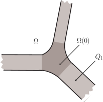
Figure 1.1: The junction of semi-infinite quantum waveguides

In this paper we present two quite different criteria for the threshold resonance and distinguish between them with the following reason. The first criterion in Section 2 with rather simple formulation is convenient to verify the absence of bounded solutions at the lower bound of the continuous spectrum but we do not see a way to apply this criterion to finding a particular bounded solution in a specific geometry. On the contrary, the second criterion in the Section 3 requiring for several definitions of auxiliary objects, can be employed to develop analytical, in particular, asymptotic methods or numerical schemes to detect and analyse concrete stabilizing (i.e. bounded but non-decaying) solutions and trapped modes with the exponential decay at infinity. At the same time, these methods and schemes may also help to disprove the threshold resonance but the latter is much more expensive in comparison with the first, absence, criterion.

Our proofs in Section 2 are conducted in such a way that they can be easily adapted for other problems, e.g., for mixed boundary conditions [7]. Nevertheless, any generalization of the whole existence criterion in Section 3 is still a fully open question.

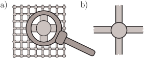
Figure 1.2: Rectangular lattice (a) and the infinite cruciform waveguide (b) to describe the boundary layer phenomenon

1.2 Statement of the spectral problem

Let $\Omega\subset\mathbb{R}^{d}$, $d\geq 2$ be a domain, by definition an open connected set, with several cylindrical outlets $Q_{1}$, …, $Q_{N}$ to infinity. We assume that $\Omega=\Omega(0)\cup Q_{1}\cup\ldots\cup Q_{N}$ where $\Omega(0)$ is a bounded domain (shaded in Fig. 1) with Lipschitz boundary, and $Q_{n}\cap Q_{k}=\varnothing$ for $n\neq k$, $Q_{n}\cap\Omega(0)=\varnothing$ for $n=1,\ldots,N$. In each outlet $Q_{n}=\omega_{n}\times[0,\infty)$ we introduce the Cartesian system $(y_{n},z_{n})$ of local coordinates with $y_{n}\in\omega_{n}$, $z_{n}\in[0,+\infty)$, where the cross-section $\omega_{n}\subset\mathbb{R}^{d-1}$ is a bounded domain with Lipschitz boundary $\partial\omega_{n}$. Note that the outlets $Q_{n}$ include their ends, i.e. $\omega_{n}\times\{0\}\subset\partial\Omega(0)$ for $n=1,\ldots,N$. We also will deal with the truncated waveguide

$$\Omega(R)=\Omega(0)\cup\bigcup_{n=1}^{N}Q_{n}(R),\quad Q_{n}(R)=\{x\in Q_{n}:z_{n}\in[0,R)\},\quad R>0.$$ (1.1)

In what follows we use the notation

$$Q_{n}^{R}=Q_{n}\setminus\overline{Q_{n}(R)}=\{x\in Q_{n}\colon z_{n}>R\},\quad R>0,$$

and the index $n$ is usually omitted in proofs related to any outlet.

We consider the spectral problem for the Laplacian $\Delta=\nabla\cdot\nabla$

$$-\Delta u=\lambda u\mbox{ in }\Omega,\quad u=0\mbox{ on }\partial\Omega,$$ (1.2)

where $\nabla=\mathop{\rm grad}\nolimits$, $\lambda$ is a spectral parameter and $\partial\Omega$ is the boundary of $\Omega$ which, for simplicity, is assumed to be Lipschitz.

The variational form of the problem (1.2) reads:

$$(\nabla u,\nabla\psi)_{\Omega}=\lambda(u,\psi)_{\Omega}\quad\forall\psi\in H^{1}_{0}(\Omega),$$ (1.3)

where $(\cdot,\cdot)_{\Omega}$ is the natural scalar product in the Lebesgue space $L^{2}(\Omega)$ and $H^{1}_{0}(\Omega)$ stands for the Sobolev space of functions vanishing at the boundary $\partial\Omega$. Since the bilinear form on the left-hand side of the integral identity (1.3) is closed and positive definite, it gives rise [4, Ch.10], [25, Ch.VIII] to an unbounded positive definite self-adjoint operator $\mathcal{A}$ in the Hilbert space $L^{2}(\Omega)$.

The Dirichlet problem on the cross-section

$$-\Delta_{y}\Phi^{n}(y)=\Lambda^{n}\Phi^{n}(y),\,y\in\omega_{n},\quad\Phi^{n}(y)=0,\,y\in\partial\omega_{n},$$ (1.4)

has the monotone and unbounded eigenvalue sequence

$$0<\Lambda_{1}^{n}<\Lambda_{2}^{n}\leq\Lambda_{3}^{n}\leq\ldots\leq\Lambda_{j}^{n}\leq\ldots\to+\infty$$

and the corresponding real eigenfunctions $\Phi_{j}^{n}\in H^{1}_{0}(\omega_{n})$, $j\in\mathbb{N}$ are subject to the orthogonality and normalization conditions

$$(\Phi_{j}^{n},\Phi_{k}^{n})_{\omega_{n}}=\delta_{j,k},\quad j,k\in\mathbb{N},$$ (1.5)

where $\delta_{j,k}$ is the Kronecker symbol and ${\mathbb{N}}=\{1,2,3,\ldots\}$.

It is known that the continuous spectrum $\sigma_{c}$ of the operator $\mathcal{A}$ is the ray $[\lambda_{\dagger},+\infty)$ where the lower bound $\lambda_{\dagger}=\min\{\Lambda_{1}^{1},\ldots,\Lambda_{1}^{N}\}>0$ coincides with the smallest among all principal (minimal) eigenvalues $\Lambda_{1}^{n}$. The total multiplicity $\varkappa:=\#\sigma_{d}$ of the discrete spectrum

$$0<\lambda_{1}<\lambda_{2}\leq\ldots\leq\lambda_{\varkappa}<\lambda_{\dagger}$$ (1.6)

of the operator $\mathcal{A}$ is known to be finite.

If a cranked waveguide belongs to $\Omega$ and is composed of two skewed semi-infinite cylinders which have the cross-sections congruent to $\omega_{1}$ and meet each other under the angle $\alpha\in(0,\pi)$, then $\varkappa\geq 1$ according to a result in [1] and the max-min principle [4, Th 10.2.2]. Furthermore, the papers [1, 18, 5, 6] and [3] give examples of arbitrary large $\varkappa$ in dimension 2 and 3, respectively. We refer the book [8] for a completed review of results on the discrete spectrum of quantum waveguides and their junctions.

1.3 Trapped modes and stabilizing solutions

Within the approach [10, 15], it is important to distinguish between stabilizing solutions and trapped modes. To explain the main difference between these kinds of bounded solutions, we consider a thin, of diameter $\varepsilon\ll 1$, finite lattice $\Upsilon^{\varepsilon}$ of quantum waveguides and its fragment

$$\Upsilon^{\varepsilon}_{\bullet}=\{x\colon\varepsilon^{-1}(x-x_{\bullet})\in\Omega(1/\varepsilon)\}$$

around the node $\upsilon^{\varepsilon}_{\bullet}=\{x\colon\varepsilon^{-1}(x-x_{\bullet})\in\Omega(0)\}$ with the center $x_{\bullet}$. To simplify formulas, we suppose for a while that all cylinders $Q_{1},\ldots,Q_{N}$ have the same cross-section $\omega$ of unit $(d-1)$-dimensional area. If in addition to the isolated eigenvalues (1.6), the operator $\mathcal{A}$ has the embedded eigenvalue $\lambda_{\dagger}$ of multiplicity ${{\bf k}}\geq 0$, then, according to [10], the Dirichlet problem in $\Upsilon^{\varepsilon}$ gets eigenvalues with the asymptotic forms

$$\begin{array}[]{l}M_{j}^{\varepsilon}=\varepsilon^{-2}\lambda_{j}+o(e^{-\delta_{j}/\varepsilon}),\quad\delta_{j}>0,\quad j=1,\ldots,\varkappa,\\ M_{k+\varkappa}^{\varepsilon}=\varepsilon^{-2}\lambda_{\dagger}+o(e^{-\delta_{\dagger}/\varepsilon}),\quad\delta_{\dagger}>0,\quad k=1,\ldots,{\bf k}.\end{array}$$ (1.7)

The corresponding eigenfunctions are localized in the vicinity of the node $\upsilon^{\varepsilon}_{\bullet}$ and become exponentially small at a distance from it.

Stabilizing solutions in $\Omega$ at the threshold $\lambda=\lambda_{\dagger}$ influence the spectrum in $\Upsilon_{\bullet}^{\varepsilon}$ in a quite different way. Indeed, eigenvalues above the rescaled, cf. (1.7), threshold $\varepsilon^{-2}\lambda_{\dagger}$ are determined through ordinary differential equations on edges of the skeleton $\Upsilon^{0}=\cap_{\varepsilon>0}\Upsilon^{\varepsilon}$ linked by certain transmission conditions at vertices of the graph $\Upsilon^{0}$. If the problem in the infinite waveguide (1.1) has no stabilizing solutions at the threshold, then the transmission conditions at the vertex $x_{\bullet}$ are nothing but the Dirichlet ones, i.e. eigenfunctions in the one-dimensional model must vanish at this vertex and, therefore, the graph edges emerging from $x_{\bullet}$ decouple. On the other hand, according to [10, 15], the existence of stabilizing solutions changes the Dirichlet conditions at $x_{\bullet}$ for some other conditions, in particular, the Kirchhoff ones like in the Pauling model [24] for the Neumann problem [13, 9]. Thereby, the main question in the framework of the dimension reduction procedure [10, 15] becomes to detect stabilizing solutions rather than all bounded solutions and the corresponding threshold resonance. The existence criterion in Section 3 makes the necessary separation of two kinds of bounded solutions in a natural way, compare Proposition 3.4 and Proposition 3.1. However, the absence criterion in Section 2 cannot directly select stabilizing solution and we provide in Section 2.4 a simple sufficient condition for absence of trapped modes but do not know an appropriate necessary condition yet.

2 An absence criterion

2.1 Formulation of the first criterion

We consider the auxiliary spectral problem with mixed boundary conditions

$$\begin{array}[]{l}-\Delta v^{R}=\mu^{R}v^{R}\mbox{ in }\Omega(R),\quad v^{R}=0\mbox{ on }\Gamma(R):=\partial\Omega(R)\cap\partial\Omega,\\ \partial_{\nu}v^{R}=0\mbox{ on }\gamma(R)=\partial\Omega(R)\setminus\partial\Omega,\end{array}$$ (2.1)

where $R\geq 0$, $\partial_{\nu}$ is the outward normal derivative, in particular, $\partial_{\nu}=\partial_{z_{n}}=\partial/\partial z_{n}$ on the truncation surface $\gamma_{n}(R)=\{x\colon y_{n}\in\omega_{n},z_{n}=R\}$.

The variational formulation of the problem (2.1) reads:

$$(\nabla v^{R},\nabla\psi)_{\Omega(R)}=\mu^{R}(v^{R},\psi)_{\Omega(R)}\quad\forall\psi\in{\mathcal{H}}^{0}_{R}$$ (2.2)

where ${\mathcal{H}}^{0}_{R}:=H^{1}_{0}(\Omega(R),\Gamma(R))$ is a subspace of functions in $H^{1}(\Omega(R))$ vanishing at $\Gamma(R)$. The problem (2.2) gives rise to unbounded positive definite and self-adjoint operator $\mathcal{A}^{R}$ in $L^{2}(\Omega(R))$. Since ${\mathcal{H}}^{0}_{R}$ is compactly embedded into $L^{2}(\Omega(R))$, the spectrum of $\mathcal{A}^{R}$ is discrete and composes the monotone unbounded sequence of eigenvalues

$$0<\mu_{1}^{R}<\mu_{2}^{R}\leq\ldots\leq\mu_{\varkappa}^{R}\leq\mu_{\varkappa+1}^{R}\leq\ldots\to+\infty\,,$$ (2.3)

where their multiplicity is taken into account. We will prove the following criterion for the threshold resonance.

Theorem 2.1.

The problem (1.2) has no threshold resonance if and only if, for some $R\geq 0$, the eigenvalue $\mu_{\varkappa+1}^{R}$ of the problem (2.1) meets the inequality $\mu_{\varkappa+1}^{R}>\lambda_{\dagger}$. Here, $\varkappa$ is the total multiplicity of the discrete spectrum $\sigma_{d}$, see (1.6).

2.2 Sufficiency

Proposition 2.2.

If the eigenvalue $\mu_{\varkappa+1}^{R}$ of the problem (2.1) meets the inequality $\mu_{\varkappa+1}^{R}>\lambda_{\dagger}$ for some $R\geq 0$, then the threshold resonance is absent in the problem (1.2).

This result coincides with Theorem 3 in [23]. Here, we only provide a short sketch of a proof. The proof is based on a simple observation, originally used in [19, 20, 2, 21] for the case $\varkappa=1$: if the threshold resonance occurs, one may construct a small compact perturbation $\mathcal{B}$ located in $\Omega(0)$, that is $\mathcal{B}u=0$ in $\Omega\setminus\Omega(0)$, with the following properties. First of all, the perturbed eigenvalues $\widehat{\mu}_{1}^{R},\ldots,\widehat{\mu}_{\varkappa}^{R}$ and $\widehat{\mu}_{\varkappa+1}^{R}$ of the operator $\widehat{\mathcal{A}}_{R}=\mathcal{A}_{R}+\mathcal{B}$ still stay, respectively, below and above the threshold $\lambda_{\dagger}$, so that one gets the Poincare inequality

$$(\widehat{\mathcal{A}}_{R}u_{0},u_{0})_{\Omega(R)}\geq\widehat{\mu}^{R}_{\varkappa+1}\|u_{0};L^{2}(\Omega(R))\|^{2}\geq\lambda_{\dagger}\|u_{0};L^{2}(\Omega(R))\|^{2},$$ (2.4)

where $u_{0}$ is orthogonal in $L^{2}(\Omega(R))$ to eigenfunctions of $\widehat{\mathcal{A}}_{R}$ corresponding to $\widehat{\mu}_{1}^{R},\ldots,\widehat{\mu}_{\varkappa}^{R}$. Then in a standard way the max-min principle, cf. [4, Theorem 10.2.2], equipped with the inequalities (2.4) and

$$\|\nabla u;L^{2}(Q_{n}^{R})\|^{2}\geq\Lambda_{1}^{n}\|u;L^{2}(Q_{n}^{R})\|^{2}\geq\lambda_{\dagger}\|u;L^{2}(Q_{n}^{R})\|^{2},$$ (2.5)

verifies that the total multiplicity of the discrete spectrum $\widehat{\sigma}_{d}$ of the operator $\widehat{\mathcal{A}}=\mathcal{A}+\mathcal{B}$ meats the inequality $\#\widehat{\sigma}_{d}\leq\varkappa$. Notice that (2.5) is a direct consequence of the Friedrichs inequality in the cross-section $\omega_{n}$.

Finally, a special choice, see cf. [19, 20, 2, 21, 23], of the perturbation $\mathcal{B}$ provides the existence of the eigenvalue $\widehat{\mu}_{\varkappa+1}<\lambda_{\dagger}$ in the discrete spectrum $\widehat{\sigma}_{d}$ of the perturbed operator $\widehat{\mathcal{A}}$. The latter contradiction completes the proof of Proposition 2.2.

2.3 Necessity

We proceed with proving that eigenvalues in the sequence (2.3) below the continuous spectrum are monotone increasing functions in $R$.

Lemma 2.3.

If the eigenvalue $\mu_{k}^{R}$ of the problem (2.1) meets the inequality $\mu_{k}^{R}<\lambda_{\dagger}$ for some $R>0$, then there exists $r_{0}>0$ such that

$$\mu_{k}^{R}<\mu_{k}^{R+r}<\lambda_{\dagger}\quad\forall r\in(0,r_{0})\,.$$

Proof. We consider the operator $\mathcal{A}^{R+r}$ in $L^{2}(\Omega(R+r))$ for small $r>0$ as a perturbation of $\mathcal{A}^{R}$ in a certain sense. For the simple eigenvalue $\mu^{R}$ (we omit the index $k$), we denote by $v^{R}$ the corresponding eigenfunction normalized in $L^{2}(\Omega(R))$. Let us accept the simplest asymptotic ansätze

$$\mu^{R+r}=\mu^{R}+r\mu^{\prime}+\ldots,$$ (2.6)

$$v^{R+r}=v^{R}+rv^{\prime}+\ldots$$ (2.7)

where the correction terms $\mu^{\prime}$ and $v^{\prime}$ are to be determined and ellipses replace small reminders to be estimated. The functions $v^{R}$ and $v^{\prime}$ defined in $\Omega(R)$, can be smoothly extended onto $\Omega\supset\Omega(R+r)$. We use the same letters for these extensions. Plugging formulas (2.6) and (2.7) into the equation for $v^{R+r}$ on $\Omega(R)$ and collecting terms of the same order in $r$ yield

$$\Delta v^{\prime}(x)+\mu^{R}v^{\prime}(x)=-\mu^{\prime}v^{R}(x),\,x\in\Omega(R)\,.$$ (2.8)

Imposing the Dirichlet condition

$$v^{\prime}(x)=0,\,x\in\Gamma(R),$$

is quite evident. The Neumann condition on $\gamma(R+r)$ can be formally transferred to $\gamma(R)$ by the Taylor formula in the variable $z$, indeed,

$$\partial_{z}v^{R+r}\big{|}_{z=R+r}=\partial_{z}v^{R}\big{|}_{z=R+r}+r\partial_{z}v^{\prime}\big{|}_{z=R+r}+\ldots=\\ =\partial_{z}v^{R}\big{|}_{z=R}+r\partial^{2}_{z}v^{R}\big{|}_{z=R}+r\partial_{z}v^{\prime}\big{|}_{z=R}+\ldots$$

We recall the Helmholtz equation for $v^{R}$ and introduce the boundary condition

$$\partial_{z}v^{\prime}(x)=-\partial_{z}^{2}v^{R}(x)=\Delta_{y}v^{R}(x)+\mu^{R}v^{R}(x),\,x\in\gamma(R)\,.$$ (2.9)

The compatibility condition in the problem (2.8)-(2.9) reads:

$$\mu^{\prime}=\mu^{\prime}(v^{R},v^{R})_{\Omega(R)}=-({\Delta}_{y}v^{R}+\mu^{R}v^{R},v^{R})_{\gamma(R)}=\\ =\|{\nabla}_{y}v^{R};L^{2}(\gamma(R))\|^{2}-\mu^{R}\|v^{R};L^{2}(\gamma(R))\|^{2}\,.$$

By the Friedrichs inequality on $\gamma(R)$, we obtain

$$\mu^{\prime}\geq\sum_{n=1}^{N}(\Lambda_{1}^{n}-\mu^{R})\|v^{R};L^{2}(\gamma_{n}(R))\|^{2}\geq(\lambda_{\dagger}-\mu^{R})\|v^{R};L^{2}(\gamma(R))\|^{2}>0.$$

If the eigenvalue $\mu^{R}$ has multiplicity $m$, calculations mainly remain the same. The leading term in the anzatz (2.7) becomes a linear combination of the corresponding eigenfunctions $v^{R}_{1}$, $v^{R}_{2}$, …, $v^{R}_{m}$ orthonormalized in $L^{2}(\Omega(R))$ with the coefficient column ${\bf c}=(c_{1},c_{2},\ldots,c_{m})^{\top}$. Repeating the above calculations with minor modifications, we observe that the correction terms $\Lambda_{1}^{\prime}$, …, $\Lambda_{m}^{\prime}$ in (2.6) are found from the system of linear algebraic equations

$${\bf A}{\bf c}=\Lambda^{\prime}{\bf c},$$

where the self-adjoint and positive definite matrix ${\bf A}$ of size $m\times m$ has the entries

$${\bf A}_{pq}=(\nabla_{y}v^{R}_{p},\nabla_{y}v^{R}_{q})_{\gamma(R)}-\mu^{R}(v^{R}_{p},v^{R}_{q})_{\gamma(R)},\,p,q=1,\ldots,m.$$

The correction terms in the asymptotic formula (2.6) for the eigenvalues $\mu_{k}^{R+r},\ldots,\mu_{k+m-1}^{R+r}$ of the problem (2.1) in $\Omega(R+r)$ involve the eigenvalues $\Lambda_{1}^{\prime}$,…, $\Lambda_{m}^{\prime}$ of ${\bf A}$ and therefore become strictly positive as in the case of simple eigenvalues. To conclude with the proof, we mention that the error estimates $|\mu_{k}^{R+r}-\mu_{k}^{R}-r\mu_{k}^{\prime}|\leq c_{k}r^{2}$ for $r\in(0,r_{k})$ are derived in a classical way, see [12, Ch.7, §6.5], because one can readily construct “almost identical” diffeomorphism between the domains $\Omega(R+r)$ and $\Omega(R)$, which is identical inside $\Omega(R-1)$ and coincides with the shift operator near the faces $\gamma_{n}(R)$. We omit here the corresponding simple and routine computations. $\Box$

Now assume that the condition on $\mu_{\varkappa+1}^{R}$ in Theorem 2.1 is violated. This means that, in particular, $\mu^{R}=\mu_{\varkappa+1}^{R}<\lambda_{\dagger}$ for all $R>2$. We normalize the corresponding eigenfunction $v_{R}$ as follows:

$$\|v^{R};L^{2}(\Omega(2))\|=1.$$ (2.10)

We are going to verify that there exists a monotone unbounded sequence $\{R_{j}\}_{j\in\mathbb{N}}$ such that $v^{R_{j}}$ converges in a certain sense to a non-trivial bounded solution $v^{\infty}$ of the problem (1.2) with parameter $\mu^{\infty}=\lim\mu^{R_{j}}$ as $j\to+\infty$. To this end, we use the decomposition

$$\chi_{1}(x)v^{R}(x)=\chi_{1}(x)w_{n}^{R}(z_{n})\Phi_{1}^{n}(y_{n})+v^{R}_{\perp}(x)\quad\mbox{in}\quad Q_{n},\quad n=1,\ldots,N$$ (2.11)

and treat its ingredients $w_{n}^{R}$ and $v_{\perp}^{R}$ in a different way.

Let us recall that $\Phi_{1}^{n}$ is the first eigenfunction of the Dirichlet Laplacian in $\omega_{n}$ and $\|\Phi_{1}^{n};L^{2}(\omega_{n})\|=1$. Furthermore,

$$w_{n}^{R}(z_{n})=\int_{\omega_{n}}v^{R}(x)\Phi_{1}^{n}(y_{n})dy_{n},\quad\int_{\omega_{n}}v^{R}_{\perp}(y_{n},z_{n})\Phi_{1}^{n}(y_{n})dy_{n}=0.$$ (2.12)

The smooth cut-off function $\chi_{s}$ is chosen such that $0\leq\chi_{s}\leq 1$ and

$$\chi_{s}(x)=0\mbox{ if }x\in\Omega(s-1),\quad\chi_{s}(x)=\chi(z_{n}-s)\mbox{ if }z_{n}\in[s-1,s],$$

$$\chi_{s}(x)=1\mbox{ if }z_{n}\geq s,$$

with a fixed smooth function $\chi$. We will also use the difference $\mathcal{X}_{s}(x)=1-\chi_{s}(x)$. We further define $w^{R}$ as follows:

$$\chi_{1}w^{R}=\chi_{1}w_{n}^{R}\Phi_{1}^{n}\mbox{ in }Q_{n},\quad w^{R}=0\mbox{ in }\Omega(0).$$

Note that that $v^{R}_{\perp}$ in (2.12) is assumed to be zero in $\Omega(0)$.

Lemma 2.4.

There exists a positive constant $c_{1}(\Omega)$ such that

$$\|\nabla_{x}v^{R};L^{2}(\Omega(1))\|+\sum_{n=1}^{N}\|v^{R};L^{2}(\gamma_{n}(1))\|\leq c_{1}(\Omega)\,.$$ (2.13)

Proof. From the integral identity (2.2) we derive the relation

$$\|\nabla v^{R};L^{2}(\Omega(1))\|^{2}\leq\|\nabla(\mathcal{X}_{2}v^{R});L^{2}(\Omega(2))\|^{2}=\\ =\mu^{R}\|\mathcal{X}_{2}v^{R};L^{2}(\Omega(2))\|^{2}+\|v^{R}\nabla\mathcal{X}_{2};L^{2}(\Omega(2))\|^{2}\leq c_{1}(\Omega)\,.$$

The last inequality follows from (2.10). The standard trace inequality provides the desired estimate of the norm $\|v^{R};L^{2}(\gamma_{n}(1))\|$ as well. $\Box$

Separation of variables gives

$$-\partial^{2}_{z_{n}}w_{n}^{R}(z_{n})=(\mu^{R}-\Lambda_{1}^{n})w_{n}^{R}(z_{n})\mbox{ for }z_{n}>1,\quad\partial_{z_{n}}w_{n}^{R}(R)=0\,.$$ (2.14)

Moreover, formulas (2.11) and (2.13) assure that $|w_{n}^{R}(1)|\leq c_{1}(\Omega)$. A solution of the problem (2.14) takes the form

$$w_{n}^{R}(z_{n})=a_{n}^{R}(e^{-\alpha_{n}(R)z_{j}}+e^{-2\alpha_{n}(R)R}e^{\alpha_{n}(R)z_{n}})$$

where $\alpha_{n}(R)=\sqrt{\Lambda_{1}^{n}-\mu^{R}}$. Thus,

$$|a_{n}^{R}|\leq c_{2}(\Omega),\quad n=1,\ldots,N,\,\,R>2.$$ (2.15)

Now we examine the function $v_{\perp}^{R}$ in (2.11). First, the Poincare inequality

$$\|\nabla_{y_{n}}v^{R}_{\perp}(\cdot,z_{n});L^{2}(\omega_{n})\|^{2}\geq\Lambda_{2}^{n}\|v^{R}_{\perp}(\cdot,z_{n});L^{2}(\omega_{n})\|^{2},\quad z_{n}>0,$$ (2.16)

is valid due to the orthogonality condition in (2.12). Furthermore, $v^{R}_{\perp}$ is a solution of the problem

$$-\Delta v^{R}_{\perp}-\mu^{R}v^{R}_{\perp}=[\Delta,\chi_{1}](v^{R}-w^{R})=:f^{R}\mbox{ in }\Omega(R),$$ (2.17)

$$v^{R}_{\perp}=0\mbox{ on }\Gamma(R),\quad\partial_{n}v^{R}_{\perp}=0\mbox{ on }\gamma(R),$$ (2.18)

where $[\Delta,\chi_{1}]$ is the commutator of the Laplacian and the cut-off function $\chi_{1}$ (a first-order differential operator). Obviously,

$$\mathop{\rm supp}\nolimits f^{R}\subset\Omega(1)\setminus\Omega(0),\quad\|f^{R};L^{2}(\Omega(R))\|\leq c_{3}(\Omega).$$ (2.19)

We fix a parameter $\beta=\beta(\Omega)$ such that

$$0<\beta<\frac{1}{2}\left(\min_{1\leq n\leq N}\Lambda_{2}^{n}-\lambda_{\dagger}\right)$$ (2.20)

and introduce the weight function $T_{\beta}$,

$$T_{\beta}(x)=1\mbox{ for }x\in\Omega(1),\quad T_{\beta}(x)=e^{\beta(z_{n}-1)}\mbox{ for }z_{n}\geq 1\,.$$

We also need the weighted Sobolev and Lebesgue spaces $W^{1}_{\beta}(\Omega)$ and $L^{2}_{\beta}(\Omega)$ with the following norms:

$$\|v;W^{1}_{\beta}(\Omega)\|=\|T_{\beta}v;H^{1}(\Omega)\|\quad\mbox{and}\quad\|v;L^{2}_{\beta}(\Omega)\|=\|T_{\beta}v;L^{2}(\Omega)\|.$$

If $\Omega$ is replaced with $\Omega(R)$ in these definitions, we obtain the spaces $W^{1}_{\beta}(\Omega(R))$ and $L^{2}_{\beta}(\Omega(R))$ which coincide algebraically and topologically with $H^{1}(\Omega(R))$ and $L^{2}(\Omega(R))$, respectively.

Lemma 2.5.

For all $R>1$, the function $v_{\perp}^{R}$ enjoys the estimate

$$\|v_{\perp}^{R};W^{1}_{\beta}(\Omega(R))\|\leq c_{\perp}(\Omega).$$ (2.21)

Proof. The function $T_{\beta}^{2}v_{\perp}^{R}$ falls into the space $\mathcal{H}_{R}^{0}$ and can be inserted as a test function into the integral identity for the problem (2.17)-(2.18). Thus, we have

$$(\nabla v^{R}_{\perp},\nabla(T_{\beta}^{2}v^{R}_{\perp}))_{\Omega(R)}=\mu^{R}\|T_{\beta}v^{R}_{\perp};L^{2}(\Omega(R))\|^{2}+(f^{R},T^{2}_{\beta}v^{R}_{\perp})_{\Omega(R)}\,.$$ (2.22)

The left-hand side is equal to

$$(\nabla v^{R}_{\perp},\nabla(T_{\beta}^{2}v^{R}_{\perp}))_{\Omega(R)}=\|\nabla(T_{\beta}v^{R}_{\perp});L^{2}(\Omega(R))\|^{2}-\|v^{R}_{\perp}\nabla(T_{\beta});L^{2}(\Omega(R))\|^{2}$$ (2.23)

and, in view of (2.16) and (2.20), gets the below bound

$$\left(\min_{1\leq n\leq N}\Lambda_{2}^{n}-\beta\right)\|T_{\beta}v^{R}_{\perp};L^{2}(\Omega(R))\|^{2}\geq(\beta+\lambda_{\dagger})\|T_{\beta}v^{R}_{\perp};L^{2}(\Omega(R))\|^{2}.$$

Hence, we deduce that

$$\|T_{\beta}v^{R}_{\perp};L^{2}(\Omega(R))\|^{2}\leq\beta^{-1}(T^{2}_{\beta}f^{R},v^{R}_{\perp})_{\Omega(R)}\leq\\ \leq\beta^{-1}\|T^{2}_{\beta}f^{R};L^{2}(\Omega(R))\|\|v^{R}_{\perp};L^{2}(\Omega(1))\|\,.$$ (2.24)

Relations (2.19), (2.22)-(2.24) show that the product $T_{\beta}v^{R}_{\perp}$ also enjoys the inequality

$$\|\nabla(T_{\beta}v^{R}_{\perp});L^{2}(\Omega(R))\|^{2}\leq c_{4}(\Omega)$$

with some constant $c_{4}(\Omega)$ and, therefore, the inequality (2.21) holds true. $\Box$

Now, for $x\in\Omega(R)$, we determine the function

$$\widehat{v}^{R}=\mathcal{X}_{R}\big{(}v^{R}-\chi_{1}w^{R}\big{)}=\mathcal{X}_{1}v^{R}+\mathcal{X}_{R}v^{R}_{\perp}\,,$$ (2.25)

and extend it by zero onto the whole domain $\Omega$. First of all,

$$\|\widehat{v}^{R};W^{1}_{\beta}(\Omega)\|\leq\widehat{c}(\Omega).$$ (2.26)

The equation

$$-\Delta\widehat{v}^{R}-\mu^{R}\widehat{v}^{R}=[\Delta,\chi_{1}]w^{R}+[\Delta,\mathcal{X}_{R}]v^{\perp}=:g^{R}+h^{R}$$ (2.27)

in the variational form becomes

$$(\nabla\widehat{v}^{R},\nabla\psi)_{\Omega}-\mu^{R}(\widehat{v}^{R},\psi)_{\Omega}=(g^{R},\psi)_{\Omega}+(h^{R},\psi)_{\Omega}\quad\forall\psi\in C^{\infty}_{0}(\Omega).$$ (2.28)

We are going to perform the limit passage $R\to+\infty$ in (2.28). Since $\mu^{R}$ is non-decreasing function in $R$, it has a limit,

$$\lim_{R\to\infty}\mu^{R}=\mu^{\infty}\leq\lambda_{\dagger}.$$

The relations (2.26) and (2.15) allows us to find a monotone unbounded sequence $\{R_{k}\}$ such that

$$\widehat{v}^{R_{k}}\to\widehat{v}^{\,\infty}\quad\mbox{weakly in}\quad W^{1}_{\beta}(\Omega),$$

$$\widehat{v}^{R_{k}}\to\widehat{v}^{\,\infty}\quad\mbox{strongly in}\quad L^{2}(\Omega(2)),$$ (2.30)

$$a_{n}^{R_{k}}\to a_{n}^{\infty},\,\,\alpha_{n}(R)\to\alpha_{n}^{\infty},\,\,e^{-2\alpha_{n}(R)R}\to c_{n}^{\infty}\mbox{ for }n\leq N.$$

The function $h^{R_{k}}$ from (2.27) converges to zero weakly in $L^{2}(\Omega)$ because $\mathop{\rm supp}\nolimits h^{R_{k}}\subset\overline{\Omega(R_{k})}\setminus\Omega(R_{k}-1)$ and $\|h^{R_{k}};L^{2}(\Omega)\|\leq c(\Omega)$. The function $g^{R_{k}}$ is supported in $\overline{\Omega(1)}\setminus\Omega(0)$ and, in view of (2.30), uniformly converges to $[\Delta,\chi_{1}]w^{\infty}$ where

$$w^{\infty}(x)=a_{n}^{\infty}(e^{-\alpha_{n}^{\infty}z_{n}}+c_{n}^{\infty}e^{\alpha_{n}^{\infty}z_{n}})\Phi_{1}^{n}(y_{n})\mbox{ in }Q_{n}.$$

Note that there appear three options:

1) $a_{n}^{\infty}=0\,\Longrightarrow\,w^{\infty}(x)=0$ for $x\in Q_{n}$;

2) $a_{n}^{\infty}\neq 0$ and $\alpha_{n}^{\infty}\neq 0\,\Longrightarrow\,c_{n}^{\infty}=0$ and $w^{\infty}(x)=a_{n}^{\infty}e^{-\alpha_{n}^{\infty}z_{n}}\Phi_{1}^{n}(y_{n})$ for $x\in Q_{n}$;

3) $a_{n}^{\infty}\neq 0$ and $\alpha_{n}^{\infty}=0\,\Longrightarrow\,w^{\infty}(x)=a_{n}^{\infty}(1+c_{n}^{\infty})\Phi_{1}^{n}(y_{n})$ for $x\in Q_{n}$.

The function $\widehat{v}^{\,\infty}$ is a solution of the problem

$$(\nabla\widehat{v}^{\,\infty},\nabla\psi)_{\Omega}-\mu^{\infty}(\widehat{v}^{\,\infty},\psi)_{\Omega}=([\Delta,\chi_{1}]w^{\infty},\psi)_{\Omega}\quad\forall\psi\in C^{\infty}_{0}(\Omega)$$

and, therefore, $v^{\infty}=\widehat{v}^{\,\infty}+\chi_{1}w^{\infty}$ becomes a bounded solution of the problem (1.2) with the $\lambda=\mu^{\infty}$. Taking into account formula (2.25) together with relation (2.30) and using that $\mathcal{X}^{R}=1$ on $\Omega(R)$ for $R>2$, we obtain

$$\|v^{\infty};L^{2}(\Omega(2))\|=\|\widehat{v}^{\,\infty}+\chi_{1}w^{\infty};L^{2}(\Omega(2))\|=\\ =\lim_{R_{k}\to+\infty}\|\widehat{v}^{R_{k}}+\chi_{1}w^{R_{k}};L^{2}(\Omega(2))\|=\lim_{R_{k}\to+\infty}\|v^{R_{k}};L^{2}(\Omega(2))\|=1\,.$$

Thus, $v^{\infty}\neq 0$.

If $\mu^{\infty}<\lambda_{\dagger}$, then $\mu^{\infty}$ becomes $(\varkappa+1)$-th eigenvalue of the problem (1.2) that contradicts our assumptions. If $\mu^{\infty}=\lambda_{\dagger}$ we obtain the desired result.

Now we are in position to formulate the obtained assertion.

Proposition 2.6.

If $\mu^{R}=\mu_{\varkappa+1}^{R}<\lambda_{\dagger}$ for all $R\geq 0$, then there exists threshold resonance in the problem (1.2).

Propositions 2.2 and 2.6 readily lead to Theorem 2.1.

2.4 A sufficient condition for the absence of trapped modes

Let us assume that

$$\lambda_{\dagger}=\Lambda_{1}^{1}=\Lambda_{1}^{2}=\ldots=\Lambda_{1}^{\bf n}<\Lambda_{1}^{\bf n+1}\leq\ldots\leq\Lambda_{1}^{N}.$$ (2.31)

A characteristic feature of a trapped mode $u\in H^{1}_{0}(\Omega)$ looks as follows:

$$\int_{\omega_{n}}u(y_{n},0)\Phi_{1}^{n}(y_{n})dy_{n}=0,\quad n=1,\ldots,{\bf n}.$$ (2.32)

These equalities are supported by the orthogonality conditions in (1.5) and the absence of the term $C_{n}\Phi_{1}^{n}(y_{n})$ in the Fourier series of the decaying solution $u$ in the outlet $Q_{n}$.

Let us consider the spectral problem: to find an eigenpair $\{\mu,v^{0}\}\in\mathbb{R}\times H^{1}_{0}(\Omega(0),\Gamma(0))_{\perp}$ such that

$$(\nabla v^{0},\nabla\psi)_{\Omega(0)}=\mu(v^{0},\psi)\quad\forall\psi\in H^{1}_{0}(\Omega(0),\Gamma(0))_{\perp}.$$ (2.33)

Here, $H^{1}_{0}(\Omega(0),\Gamma(0))_{\perp}$ is a subspace of functions in $H^{1}(\Omega(0))$ which vanish at the surface $\Gamma(0)=\partial\Omega(0)\cap\partial\Omega$ and enjoy the orthogonality conditions (2.32). The differential formulation of this problem involves the equations (2.32) and

$$-\Delta v^{0}(x)=\mu v^{0}(x),\quad x\in\Omega(0),\quad v^{0}(x)=0,\quad x\in\Gamma(0),$$

$$\partial_{\nu}v^{0}(x)=0,\quad x\in\gamma_{n}(0),\quad n={\bf n}+1,\ldots,N,$$

$$\partial_{\nu}v^{0}(x)=C_{n}\Phi_{1}^{n}(y_{n}),\quad x\in\gamma_{n}(0),\quad n=1,\ldots,{\bf n},$$

where the constants $C_{1},\ldots,C_{\bf n}$ are unfixed.

Theorem 2.7.

Let $u$ be a bounded solution of the problem (1.2) at the threshold $\lambda=\lambda_{\dagger}$. If the first eigenvalue of the problem (2.33) enjoys the relation $\mu_{1}>\lambda_{\dagger}$, then $u$ does not decay at infinity and, therefore, is nothing but a non-trivial stabilizing solution.

Proof. By the theorem on unique continuation, $u$ cannot vanish everywhere in $\Omega(0)$ and, hence, the Friedrichs inequality serving for the problem (2.33) gives us the formula

$$\|\nabla u;L^{2}(\Omega(0)))\|^{2}\geq\mu_{1}\|u;L^{2}(\Omega(0))\|^{2}>\lambda_{\dagger}\|u;L^{2}(\Omega(0))\|^{2}.$$

Taking (2.5) with $R=0$ into account, we come across a contradiction with the integral identity (1.3) where $\psi=u$. $\Box$

2.5 Remarks on some known examples

The papers [19] and [20] deal with the symmetric ${\sf T}$- and ${\sf Y}$-shaped planar quantum waveguides where multiplicity of the discrete spectrum is 1 while the second eigenvalue of the problem (2.1) in the smallest node $\Omega(0)$, the unit square $\square$ and the equilateral triangle $\triangle$ (shaded in Fig. 3, a and b), respectively, is strictly bigger than $\lambda_{\dagger}=\pi^{2}$. In this way, the simplest $(\varkappa=1)$ version of Proposition 2.2 applies.

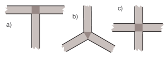
Figure 2.1: T-, Y- and X-shaped waveguides

Considering the cruciform waveguide composed from unit circular cylinders, perpendicular to each other, the paper [2] demonstrate that $\varkappa=1$ and the eigenvalue $\lambda_{2}^{R}$ of the problem (2.1) with a big $R$ satisfies the inequality $\lambda_{2}^{R}>\lambda_{\dagger}$, cf. Proposition 2.2. However, for the planar cruciform waveguide made from two perpendicular unit strips, the Neumann problem in the square $\square$ (shaded in Fig. 3, c) has the eigenvalues $\lambda_{1}^{0}=0$, $\lambda_{2}^{0}=\lambda_{3}^{0}=\pi^{2}=\lambda_{\dagger}$. In [21, §4] and [23, §3] certain symmetrization tricks were proposed to reject the threshold resonance. At the same time, Proposition 2.5 shows that $\lambda_{2}^{R}>\pi^{2}$ when $R>R_{2}>0$.

3 An existence criterion

3.1 The Steklov-Poincare operator

To turn the problem (1.2) with the threshold spectral parameter $\lambda=\lambda_{\dagger}$ in the infinite domain $\Omega$ into a problem posed in a finite domain, the Steklov–Poincare operator, cf. [11, 26], is often used. It is expressed through solutions of the Dirichlet problem in the semi-infinite cylinder

$$-\Delta U^{n}=\lambda_{\dagger}U^{n}\mbox{ in }Q_{n},\quad U^{n}=0\mbox{ on }\Gamma_{n}:=\partial Q_{n}\cap\partial\Omega,$$

$$U^{n}(y,0)=F^{n}(y)\mbox{ for }y\in\omega_{n}.$$

Traditionally, this operator acts as follows: $F^{n}\mapsto\partial_{z}U^{n}\big{|}_{z=0}$.

The Fourier method provides an explicit solution of (3.1) so that the operator takes form

$$\sum_{p=1}^{\infty}a_{p}^{n}\Phi_{p}^{n}=F^{n}\mapsto T^{n}F^{n}=-\sum_{p=1}^{\infty}\kappa_{p}^{n}a_{p}^{n}\Phi_{p}^{n},$$ (3.2)

where $\kappa_{p}^{n}=(\Lambda_{p}^{n}-\lambda_{\dagger})^{1/2}>0$ for $\Lambda_{p}^{n}>\lambda_{\dagger}$ but $\kappa_{1}^{n}=-i$ for $n=1,\ldots,{\bf n}$, i.e., in the case $\Lambda_{1}^{n}=\lambda_{\dagger}$ (see [16, §2] for the latter).

If $n={\bf n}+1,\ldots,N$ and $\lambda_{\dagger}$ stays below the continuous spectrum $[\Lambda_{1}^{n},+\infty)$ of the problem in $Q_{n}$, and

$$(T^{n}F^{n})(y)=\partial_{z}U^{n}(y,0),$$ (3.3)

where $U^{n}\in H^{1}(Q_{n})$, is the unique solution of (3.1) with the finite Dirichlet integral. In the case $n=1,\ldots,{\bf n}$ formula (3.3) is still valid but $U^{n}$ is a solution to the problem (3.1) with proper threshold radiation conditions, see Remark 3.2.

The Fourier method shows that the mapping $T^{n}:H^{1}_{0}(\omega_{n})\to L^{2}(\omega_{n})$ is continuous. At the same time,

$$(T^{n}F^{n},G^{n})_{\omega_{n}}=-\sum_{p=1}^{\infty}\kappa^{n}_{p}a^{n}_{p}\overline{b^{n}_{p}},$$ (3.4)

where $\{a^{n}_{p}\}$ and $\{b^{n}_{p}\}$ are the Fourier coefficients of $F^{n}$ and $G^{n}$, respectively. For $n={\bf n}+1,\ldots,N$, the relation (3.4) recognizes $T^{n}$ as a negative operator in the Hilbert space $H^{1/2}_{00}(\omega_{n})$, see [14, §1.11], with the norm

$$\|\Psi;H^{1/2}_{00}(\omega_{n})\|=(\|\Psi;H^{1/2}(\omega_{n})\|^{2}+\|\rho^{-1/2}\Psi;L^{2}(\omega_{n})\|^{2})^{1/2},$$ (3.5)

where $\rho=\mathop{\rm dist}\nolimits(y,\partial\omega_{n})$ and $H^{1/2}(\omega_{n})$ is the standard Sobolev-Slobodetskii space. Notice that the last weighted norm in (3.5) originates in the Dirichlet condition on $\partial\omega_{n}$ for the eigenfunctions $\Phi^{n}_{p}$. The operator $T^{n}$ with $n=1,\ldots,{\bf n}$ gets a skew-symmetric component on the one-dimensional subspace $\mathcal{L}^{n}$ spanned over the first eigenfunction $\Phi_{1}^{n}$ of the problem (1.4).

Eventually, in the case of the source term $f\in L^{2}(\Omega)$ with $\mathop{\rm supp}\nolimits f\subset\overline{\Omega(0)}$ a solution of the problem

$$-\Delta u^{0}-\lambda_{\dagger}u^{0}=f\mbox{ in }\Omega(0),\quad u^{0}=0\mbox{ on }\Gamma(0),$$ (3.6)

$$\partial_{z}u^{0}=T^{n}u^{0}\mbox{ on }\omega_{n}(0),\quad n=1,\ldots,N.$$

is nothing but the restriction on $\Omega(0)$ of a solution of the problem

$$-\Delta u-\lambda_{\dagger}u=f\mbox{ in }\Omega,\quad u=0\mbox{ on }\partial\Omega$$ (3.7)

with the threshold radiation conditions (3.22).

3.2 Symmetrization of the Steklov-Poicare operator

As was mentioned above, the problem (3.6) inherits all properties of the problem (3.7), in particular, it becomes uniquely solvable if and only if the same property is attributed to (3.7). However, a convenient application of the reduced problem in $\Omega(0)$ needs its unique solvability which is clearly absent in the presence of the threshold resonance. In this way, it was proposed in [16] to introduce the positive definite symmetric operator

$$F^{n}\mapsto M^{n}F^{n}=\sum_{p=1}^{\infty}|\kappa_{p}^{n}|a_{p}^{n}\Phi_{p}^{n}$$ (3.8)

and consider the auxiliary problem

$$-\Delta w-\lambda_{\dagger}w=0\mbox{ in }\Omega(0),\quad w=0\mbox{ on }\Gamma(0),$$ (3.9)

$$\partial_{z}w-iM^{n}w=g^{n}\mbox{ on }\omega_{n}(0),\quad n=1,\ldots,N.$$

The weak formulation of this problem reads: to find $w\in\mathcal{H}^{0}_{0}$, see Section 2.2, such that

$$(\nabla w,\nabla v)_{\Omega(0)}-\lambda_{\dagger}(w,v)_{\Omega(0)}-i\langle{\bf M}w,v\rangle=\langle g,v\rangle\quad\forall v\in\mathcal{H}^{0}_{0}.$$ (3.10)

Here, ${\bf M}=\mathop{\rm diag}\nolimits\{M^{1},M^{2},\ldots,M^{N}\}$, $g=(g^{1},g^{2},\ldots,g^{N})$ and $\langle\,,\rangle$ is the extension of the scalar product in ${\bf L}:=L^{2}(\omega_{1}(0))\oplus\ldots\oplus L^{2}(\omega_{n}(0))$ up to the duality between the space

$${\bf H}=H^{1/2}_{00}(\omega_{1}(0))\oplus\ldots\oplus H^{1/2}_{00}(\omega_{N}(0))$$

and its adjoint ${\bf H}^{*}:=H^{-1/2}_{00}(\omega_{1}(0))\oplus\ldots\oplus H^{-1/2}_{00}(\omega_{N}(0))$.

As was proved in [16, Lemma 2.2] and can be easily verified on the basis of the theorem on unique continuation, in view of the presence of the skew-symmetric sesquilinear form $i\langle{\bf M}w,v\rangle$ the problem (3.10) with any $g\in{\bf H}^{*}$ has a unique solution $w\in\mathcal{H}^{0}_{0}$ and the following estimate is valid:

$$\|w;\mathcal{H}^{0}_{0}\|\leq c\|g;{\bf H}^{*}\|.$$ (3.11)

3.3 The fictitious scattering operator.

Following [16], we introduce an artificial object, a unitary operator ${\bf S}$ in ${\bf L}$ which can be directly constructed through solutions of the uniquely solvable problem (3.9) and becomes an identificator of all bounded solutions at the threshold, see Theorem 3.5.

Let ${\bf M}^{1/2}$ be the positive square root of the positive self-adjoint operator ${\bf M}$ in (3.8). For any $\psi\in{\bf L}$, we denote by $w(\psi)\in\mathcal{H}^{0}_{0}$ the (unique) solution of the problem (3.10) with the specific right-hand side

$$g=-2^{1/2}i{\bf M}^{1/2}\psi\in{\bf H}^{*}$$ (3.12)

and set

$${\bf S}\psi=i\psi-2^{1/2}i{\bf M}^{1/2}w(\psi)|_{\omega(0)}\in{\bf L}\,,$$ (3.13)

where $\omega(0)=\omega_{1}(0)\times\ldots\times\omega_{N}(0)$. In view of the estimate (3.11) and the properties of the operator ${\bf M}$ we see that (3.13) is a continuous operator in ${\bf L}$. Moreover, in [16, Theorem 2.1] it is verified that, owing to the special choice (3.12) of the right-hand side in (3.9), ${\bf S}$ is a unitary operator in ${\bf L}$.

3.4 The criterion for trapped modes

Let ${\bf L}_{0}$ be the subspace

$$\{\psi\in{\bf L}: \psi|_{\omega_{n}(0)}=c_{n}\Phi_{1}^{n},n=1,\ldots,{\bf n},c_{n}\in\mathbb{C},$$

$$\psi|_{\omega_{n}(0)}=0,n={\bf n}+1,\ldots,N\}$$

and let ${\bf L}_{\perp}={\bf L}\ominus{\bf L}_{0}$ be the orthogonal complement of (3.4). Denoting the orthogonal projectors on ${\bf L}_{0}$ and ${\bf L}_{\perp}$ by ${\bf P}_{0}$ and ${\bf P}_{\perp}$, respectively, we define the operator

$${\bf S}_{\perp}={\bf P}_{\perp}{\bf S}{\bf P}_{\perp}:{\bf L}_{\perp}\to{\bf L}_{\perp}.$$ (3.15)

In [16, Theorem 3.1] it is verified that the mapping

$${\bf D}_{tr}\ni u\mapsto\psi=2^{-1/2}(1+i){\bf M}^{1/2}u|_{\omega(0)}\in\ker({\bf S}_{\perp}-\mathop{\rm Id}\nolimits_{\perp})$$

is a bijection where ${\bf D}_{tr}$ is the subspace of trapped modes in the problem (1.2) at the threshold $\lambda=\lambda_{\dagger}$ and $\ker({\bf S}_{\perp}-\mathop{\rm Id}\nolimits_{\perp})$ is the eigenspace of the operator (3.15) for its eigenvalue 1. This fact readily establishes the existence criterion for trapped modes.

Proposition 3.1.

There holds

$$\dim{\bf D}_{tr}=\dim\ker({\bf S}_{\perp}-\mathop{\rm Id}\nolimits_{\perp}),$$ (3.16)

i.e. a trapped mode exists if and only if the operator (3.15) has the eigenvalue 1.

It should be mentioned that

$$\begin{array}[]{l}\psi\in\ker({\bf S}_{\perp}-\mathop{\rm Id}\nolimits_{\perp})\quad\Rightarrow\quad\|\psi;{\bf L}\|^{2}=\|{\bf S}\psi;{\bf L}\|^{2}=\|{\bf P}_{\perp}{\bf S}\psi;{\bf L}\|^{2}+\\ +\|{\bf P}_{0}{\bf S}\psi;{\bf L}\|^{2}=\|\psi;{\bf L}\|^{2}+\|{\bf P}{\bf S}\psi;{\bf L}\|^{2}\quad\Rightarrow\quad{\bf P}{\bf S}\psi=0.\end{array}$$ (3.17)

In other words, $\psi\in\ker({\bf S}_{\perp}-\mathop{\rm Id}\nolimits_{\perp})$ is an eigenfunction of the intact fictitious scattering operator ${\bf S}$ corresponding to the eigenvalue 1.

3.5 Threshold radiation conditions and the threshold scattering matrix

At the threshold $\lambda_{\dagger}$ the standing $\Phi_{1}^{n}(y_{n})$ and resonance $y_{n}\Phi_{1}^{n}(y_{n})$ waves occur in the outlets $Q_{n}$, $n=1,\ldots,{\bf n}$. These waves cannot be classified by classical Sommerfeld radiation principle because of their null wave number. In order to define a unitary and symmetric scattering matrix at the threshold, we follow [22, Ch.5, §3], and introduce the couples of linear in $z_{n}$ waves

$$w_{n}^{in}(x)=\chi(z_{n})2^{-1/2}(z_{n}+i)\Phi^{n}_{1}(y_{n}),\quad w_{n}^{out}(x)=\chi(z_{n})2^{-1/2}(z_{n}-i)\Phi_{1}^{n}(y_{n})$$ (3.18)

where the superscripts mean “incoming” and “outgoing”. The linear combinations (3.18) of the resonance and standing waves emerging at the threshold possess the remarkable properties:

$$w_{n}^{in}(x)=\overline{w_{n}^{out}(x)}$$ (3.19)

and

$$\begin{array}[]{l}q_{n}(w_{n}^{in},w_{n}^{in})=-i,\quad q_{n}(w_{n}^{out},w_{n}^{out})=i,\\ q_{j}(w_{n}^{in},w_{n}^{out})=-\overline{q_{n}(w_{n}^{out},w_{n}^{in})}=0\end{array}$$ (3.20)

with the sesquilinear and anti-Hermitian form

$$q_{n}(u,v)=\int_{\omega_{n}}\big{(}\overline{v(x)}\partial_{z_{n}}u(x)-u(x)\overline{\partial_{z_{n}}v(x)}\big{)}\big{|}_{z_{n}=R}dy_{n}$$ (3.21)

which appears as a surface integral in the Green formula on the truncated waveguide (1.1) and, therefore, is independent of $R>1$ for waves (3.18) and their linear combinations.

Remark 3.2.

The threshold radiation condition for the problem (3.6) reads

$$u-\sum_{n=1}^{\bf n}c_{n}w_{n}^{out}\in H^{1}(\Omega)$$ (3.22)

where ${\bf n}$ is defined in (2.31), $w_{n}^{out}$ is the outgoing wave in (3.18) and $c_{1},\ldots,c_{\bf n}$ are some coefficients. Conditions of type (3.22) have been introduced in [22, Ch. 5], as well as their straight-forward modifications for the threshold inside the continuous spectrum (the eigenvalues $\Lambda_{p}^{n}$ of the model problem (1.4) with $p\geq 2$). The corresponding problems always inherit all important properties of the problems outside the thresholds.

As was demonstrated in [22, §3 Ch.5] and, e.g., [17], the relation (3.20) and (3.19) are sufficient to guarantee the existence of the special solutions

$$Z_{n}(x)=w_{n}^{in}(x)+\sum_{k=1}^{{\bf n}}{\bf s}_{kn}w_{k}^{out}(x)+\widetilde{Z}_{n}(x)$$ (3.23)

to the problem (1.2) with $\lambda=\lambda_{\dagger}$ as well as the unitary and symmetry properties of the threshold scattering matrix ${\bf s}$ composed of the coefficients ${\bf s}_{kn}$, $k,n=1,\ldots,{\bf n}$, in (3.23). Note that $Z_{n}(x)$ decays in the outlets $Q_{{\bf n}+1},\ldots,Q_{N}$ only but the reminder $\widetilde{Z}_{n}$ does in all outlets.

Remark 3.3.

The form (3.21) induces an indefinite metrics in the $2{\bf n}$-dimensional subspace $\mathcal{W}$ of polynomial waves, and, of course, the above-mentioned basis in $\mathcal{W}$ is not unique. For example, the waves

$$\begin{array}[]{l}{\bf w}_{n}^{in}(x)=\chi(z_{n})2^{-1/2}e^{i\psi}(1-iz_{n})\Phi_{1}^{n}(y_{n}),\\ {\bf w}_{n}^{out}(x)=\chi(z_{n})2^{-1/2}e^{-i\psi}(1+iz_{n})\Phi_{1}^{n}(y_{n})\end{array}$$ (3.24)

with $\psi\in\mathbb{R}$ verify the same relations (3.19) and (3.20) as waves (3.18). The threshold scattering matrix ${\bf s}$ initiated by incoming waves in (3.24) is equal to $e^{2i\psi}{\bf s}$. This observation will allow us to formulate in Theorem 3.4 the common criterion for the existence of trapped modes and stabilizing solutions.

3.6 The criterion for the existence of stabilizing solutions.

The following assertion can be found in the paper [19] but its proof is very simple and we reproduce it here for reader’s convenience. We also mention that other arguments in [15] and [10] had let to similar assertions expressed in different terms.

Proposition 3.4.

Dimension of the subspace ${\bf D}_{st}$ of stabilizing solutions coincides with multiplicity of the eigenvalue $-1$ of the threshold scattering matrix ${\bf s}$, i.e. $\dim{\bf D}_{st}=\dim\ker({\bf s}+\mathop{\rm Id}\nolimits_{0})$, where $\mathop{\rm Id}\nolimits_{0}$ is the unit matrix of size ${\bf n}\times{\bf n}$. If ${\bf s}c+c=0$ for a column $c\in\mathbb{C}^{\bf n}\setminus\{0\}$, then a nontrivial stabilizing solution is given by the linear combination

$$Z=c_{1}Z_{1}+\ldots+c_{\bf n}Z_{\bf n}\,.$$ (3.25)

Proof. The function (3.25) admits the decomposition

$${\displaystyle\begin{array}[]{l}Z(x)=\sum\limits_{n=1}^{{\bf n}}\Big{(}c_{n}w_{n}^{in}(x)+\sum\limits_{k=1}^{\bf n}c_{k}{\bf s}_{kn}w_{n}^{out}(x)\Big{)}+\widetilde{Z}(x)=\\ \sum\limits_{n=1}^{\bf n}c_{n}(w_{n}^{in}(x)-w_{n}^{out}(x))+\widetilde{Z}(x)=-\sqrt{2}i\sum\limits_{n=1}^{\bf n}c_{n}\chi_{n}(z_{n})\Phi_{1}^{n}(y_{n})+\widetilde{Z}(x)\,.\end{array}}$$ (3.26)

Here, we used the equality ${\bf s}c+c=0\in\mathbb{C}^{\bf n}$ and formulas (3.18) to observe that $Z$ is bounded and does not decay at infinity. Reading the chain (3.26) from right to left proves the equalities $c_{n}=-\sum c_{k}{\bf s}_{kn}$, $n=1,\ldots,{\bf n}$, and concludes with the whole assertion. $\Box$

In other words, the threshold scattering matrix contain the complete information on stabilizing solutions of the problem (1.2) with $\lambda=\lambda_{\dagger}$.

3.7 The fictitious scattering operator and stabilizing solutions

The function $-iZ_{n}$, see (3.23), satisfies the problem (3.9) with the right-hand side

$$g^{n}=-i\partial_{z}Z_{n}-M^{n}Z_{n}\mbox{ on }\omega_{n},\quad n=1,\ldots,{\bf n}.$$

Since ${\bf M}^{1/2}{\bf P}_{0}={\bf P}_{0}{\bf M}^{1/2}={\bf P}_{0}$ according to definitions (3.8) and (3.2), we take (3.23) into account and obtain

$${\bf P}_{0}g^{n}=-2^{1/2}i{\bf e}_{n}\Phi_{1}^{n}\quad\mbox{where}\quad{\bf e}_{n}=(\delta_{1,n},\delta_{2,n},\ldots,\delta_{N,n}).$$ (3.27)

Comparing (3.27) with (3.12) and recalling (3.4) yield

$${\bf P}_{0}{\bf S}{\bf P}_{0}\psi=i\psi-2^{1/2}{\bf M}^{1/2}{\bf P}_{0}Z|_{\omega(0)}=i\psi-2^{1/2}(i2^{-1/2}\psi-i2^{-1/2}{\bf s}\psi)=i{\bf s}\psi$$

where $Z$ is the linear combination (3.25) and

$$\psi=(c_{1}\Phi_{1}^{1},\ldots,c_{\bf n}\Phi_{1}^{\bf n},0,\ldots,0),\quad{\bf s}\psi=\sum_{k=1}^{n}c_{k}({\bf s}_{1k}\Phi_{1}^{1},\ldots,{\bf s}_{{\bf n}k}\Phi_{1}^{\bf n},0,\ldots,0).$$

In other words, the operator

$${\bf S}_{0}={\bf P}_{0}{\bf S}{\bf P}_{0}:{\bf L}_{0}\to{\bf L}_{0}$$ (3.28)

realizes as the unitary matrix $i{\bf s}$ that allows us to reformulate the criterion in Proposition 3.3 in terms of the operator (3.28), namely

$$\dim{\bf D}_{st}=\dim\ker({\bf S}_{0}+i\mathop{\rm Id}\nolimits_{0}).$$ (3.29)

Repeating the calculations (3.17) we see that ${\bf P}_{\perp}{\bf S}\psi=0$ in the case $\psi\in\ker({\bf S}_{0}+i\mathop{\rm Id}\nolimits_{0})$ and, therefore, $\psi\in\ker({\bf S}+i\mathop{\rm Id}\nolimits)$. Thus, formulas (3.16) and (3.29) lead to the following criterion for the existence of bounded solutions of the problem (1.2) with $\lambda=\lambda_{\dagger}$, that is, for the threshold resonance.

Theorem 3.5.

The subspace ${\bf D}_{bd}={\bf D}_{tr}\cup{\bf D}_{st}$ of bounded solutions verifies the relation

$$\dim{\bf D}_{bd}=\dim\ker(\widehat{{\bf S}}-\mathop{\rm Id}\nolimits),$$

where $\mathop{\rm Id}\nolimits$ is the identify operator in ${\bf L}$ and

$$\widehat{{\bf S}}=({\bf P}_{\perp}+2^{-1/2}(1-i){\bf P}_{0}){\bf S}({\bf P}_{\perp}+2^{-1/2}(1-i){\bf P}_{0}).$$ (3.30)

We emphasize that operator (3.30) is still unitary.

4 Acknowledgments

Research is financially supported by grant № 17-11-01003 of the Russian Science Foundation.

References

• [1] Y. Avishai, D. Bessis, B. G. Giraud, G. Mantica, Quantum bound states in open geometries, Phys. Rev. B, 44 (1991) 8028–8034. DOI: 10.1103/PhysRevB.44.8028
• [2] F. L. Bakharev, S. G. Matveenko, S. A. Nazarov, The discrete spectrum of cross-shaped waveguides, St. Petersburg Mathematical J. 28 (2017) 171–180. DOI: 10.1090/spmj/1444
• [3] F. L. Bakharev, S. G. Matveenko, S. A. Nazarov, Examples of Plentiful Discrete Spectra in Infinite Spatial Cruciform Quantum Waveguides, Zeitschrift fur Analysis und ihre Anwendung, 36 (2017) 329–341. DOI: 10.4171/ZAA/1591
• [4] M.S. Birman, M.Z. Solomyak, Spectral Theory of Self-Adjoint Operators in Hilbert, Space, Reidel Publishing Company, Dordrecht, 1986.
• [5] M. Dauge, Y. Lafranche, N. Raymond, Quantum waveguides with corners, ESAIM Proc. 35 (2012) 14–45.
• [6] M. Dauge, N. Raymond, Plane waveguides with corners in the small angle limit, J. Math. Phys. 53 (2012) 123529 DOI: 10.1063/1.4769993
• [7] D.V. Evans, M. Levitin, D. Vasil’ev, Existence theorems for trapped modes, J. Fluid Mech. 261 (1994) 21–31.
• [8] P. Exner, H. Kovarik, Quantum Waveguides, Theoret. Math. Phys., vol.22, Springer, 2015.
• [9] P. Exner, O. Post, Convergence of spectra of graph-like thin manifolds, J. Geom. and Phys. 54 (2005) 77–115. DOI: 10.1063/1.2749703
• [10] D. Grieser, Spectra of graph neighborhoods and scattering, Proc. London Math. Soc. 97 (2008) 718–752. DOI: 10.1112/plms/pdn020
• [11] V. I. Lebedev, V. I. Agoshkov, Operatory Puankare–Steklova i ikh prilozheniya v analize. (Russian) [Poincaré Steklov operators and their applications in analysis] Akad. Nauk SSSR, Vychisl. Tsentr, Moscow, 1983. 184 pp.
• [12] T. Kato; Perturbation theory for linear operators, Second edition, Grundlehren der Mathematischen Wissenschaften, Band 132. Springer-Verlag, Berlin-New York, 1976. xxi+619 pp.
• [13] P. Kuchment, H. Zeng, Convergence of Spectra of Mesoscopic Systems Collapsing onto a Graph. J. of Math. Anal. and Appl. 258 (2001) 671–700. DOI: 10.1006/jmaa.2000.7415
• [14] J.-L. Lions, E. Magenes, Non-homogeneous boundary value problems and applications. Vol. I. Translated from the French by P. Kenneth. Die Grundlehren der mathematischen Wissenschaften, Band 181. Springer-Verlag, New York-Heidelberg, 1972. xvi+357 pp. DOI: 10.1007/978-3-642-65161-8
• [15] S. Molchanov, B. Vainberg, Scattering solutions in networks of thin fibers: small diameter asymptotics, Comm. Math. Phys. 273 (2007) 533–559. 10.1007/s00220-007-0220-8
• [16] S.A. Nazarov, A criterion for the existence of decaying solutions in the problem on a resonator with a cylindrical waveguide, Funct. Anal. Appl. 40 (2006) 97–107. DOI: 10.1007/s10688-006-0016-1
• [17] S.A. Nazarov, Asymptotic expansions of eigenvalues in the continuous spectrum of a regularly perturbed quantum waveguide, Theor. and Math. Phys. 167 (2011) 606–627. DOI: 10.1007/s11232-011-0046-6
• [18] S.A. Nazarov, A.V. Shanin, Trapped modes in angular joints of 2D waveguides, App. Anal. 93 (2014) 572–-582. DOI: 10.1080/00036811.2013.786046
• [19] S.A. Nazarov, Bounded solutions in a T-shaped waveguide and the spectral properties of the Dirichlet ladder, Comput. Math. and Math. Phys. 54 (2014) 1261–-1279. DOI: 10.1134/S0965542514080090
• [20] S.A. Nazarov, K. Ruotsalainen, P. Uusitalo, Asymptotics of the spectrum of the Dirichlet Laplacian on a thin carbon nano-structure, C. R. Mecanique. 343 (2015) 360–-364. DOI: 10.1016/j.crme.2015.03.001
• [21] S.A. Nazarov, The spectra of rectangular lattices of quantum waveguides, Izv. Math., 81 (2017) 29–90. DOI: 10.1070/IM8380
• [22] S.A. Nazarov, B.A. Plamenevskii, Elliptic problems in domains with piecewise smooth boundaries, Walter be Gruyter, Berlin, New York (1994).
• [23] K. Pankrashkin, Eigenvalue inequalities and absence of threshold resonances for waveguide junctions, J. of Math. Anal. and App., 449 (2017) 907–925. DOI: 10.1016/j.jmaa.2016.12.039
• [24] L. Pauling, The diamagnetic anisotropy of aromatic molecules, J. Chem. Phys. 1936. V. 4.
• [25] M. Reed, B. Simon, Methods of modern mathematical physics. I. Functional analysis. Second edition. Academic Press, Inc. [Harcourt Brace Jovanovich, Publishers], New York, 1980. xv+400 pp.
• [26] A. Quarteroni, A. Valli, Domain decomposition methods for partial differential equations. Numerical Mathematics and Scientific Computation. Oxford Science Publications. The Clarendon Press, Oxford University Press, New York, 1999. xvi+360 pp. ISBN: 0-19-850178-1