Dynamic Index Tracking and Risk Exposure Control Using Derivatives

Abstract

We develop a methodology for index tracking and risk exposure control using financial derivatives. Under a continuous-time diffusion framework for price evolution, we present a pathwise approach to construct dynamic portfolios of derivatives in order to gain exposure to an index and/or market factors that may be not directly tradable. Among our results, we establish a general tracking condition that relates the portfolio drift to the desired exposure coefficients under any given model. We also derive a slippage process that reveals how the portfolio return deviates from the targeted return. In our multi-factor setting, the portfolio’s realized slippage depends not only on the realized variance of the index, but also the realized covariance among the index and factors. We implement our trading strategies under a number of models, and compare the tracking strategies and performances when using different derivatives, such as futures and options.

Keywords: slippage, index tracking, exposure control, realized covariance, derivatives trading

JEL Classification: G11, G13

Mathematics Subject Classification (2010): 60G99, 91G20

1 Introduction

A common challenge faced by many institutional and retail investors is to effectively control risk exposure to various market factors. There is a great variety of indices designed to provide different types of exposures across sectors and asset classes, including equities, fixed income, commodities, currencies, credit risk, and more. Some of these indices can be difficult or impossible to trade directly, but investors can trade the associated financial derivatives if they are available in the market. For example, the CBOE Volatility Index (VIX), often referred to as the fear index, is not directly tradable, but investors can gain exposure to the index and potentially hedge against market turmoil by trading futures and options written on VIX.

To illustrate the benefits of having exposure to VIX, consider the 2011 U.S. credit rating downgrade by Standard and Poor’s. News of a negative outlook by S&P of the U.S. credit rating broke on April 18th, 2011. As displayed in Figure 1(a), a portfolio holding only the SPDR S&P 500 ETF (SPY) would go on to lose about 10% with a volatile trajectory for a few months past the official downgrade on August 5th, 2011. In contrast, a hypothetical portfolio with a mix of SPY (90%) and VIX (10%) would be stable through the downgrade and end up with a positive return. Figure 1(b) shows the same pair of portfolios over the year 2014. Both earned roughly the same 15% return though SPY alone was visibly more volatile than the portfolio with SPY and VIX. The large drawdowns (for example on October 15th, 2014) were met by rises in VIX, creating a stabilizing effect on the portfolio’s value.

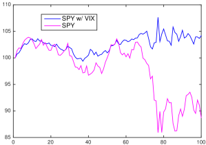
(a) April 2011 - Sept. 2011

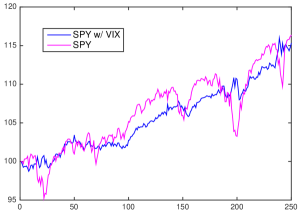
(b) Jan. 2014 - Dec. 2014

Figure 1: Hedged portfolios of SPY with 10% of wealth invested in VIX during (a) April 2011 – Sept. 2011, and (b) Jan. 2014 – Dec. 2014.

This example motivates the investigation of trading strategies that directly track VIX and other indices, or achieve any pre-specified exposure with respect to an index or market factor. Many ETFs or ETNs are advertised to provide exposure to an index by maintaining a portfolio of securities related to the index, such as futures, options, and swaps. However, some of ETFs or ETNs often miss their stated targets, and some tend to significantly underperform over time relative to the targets. One example is the Barclay’s iPath S&P 500 VIX Short-Term Futures ETN (VXX), which is also the most popular VIX exchange-traded product. The failure of VXX to track VIX is well documented (e.g. Husson and McCann (2011), Deng et al. (2012), Alexander and Korovilas (2013), and Whaley (2013)). In fact, most of these ETFs or ETNs follow a static strategy or time-deterministic allocation that does not adapt to the rapidly changing market. The problem of tracking and risk exposure control is relevant in all asset classes, and the use of derivatives is also common in other markets. For example, many investors seek exposure to gold to hedge against market turmoil. However, direct investment in gold bullion is difficult due to storage cost. In order to gain exposure, an investor may select among a number of gold derivatives, and ETFs as well as their leveraged counterparts. An analysis on the tracking properties of portfolios of gold futures and ETFs can be found in Leung and Ward (2015). For an empirical study on the tracking errors of a large collection of commodity leveraged and non-leveraged ETFs, we refer to Guo and Leung (2015) .

In this paper, we discuss a general methodology for index tracking and risk exposure control using derivatives. In Section 2, we describe the market in a continuous-time diffusion framework, and derive a condition (see Proposition 2.1) that links the exposures attainable by a derivatives portfolio. In the special case that the exposures are constant over time, the portfolio value admits an explicit expression in terms of the reference index (see Proposition 2.2). In particular, we quantify the divergence of portfolio return from the target returns of the index and its factors via the slippage process. With exposure to the index and multiple stochastic factors, the slippage process is a function of not only the realized variance of the underlying factors, but also the realized covariance among the index and factors. The slippage process derived herein reveals the potential effect of portfolio value erosion arising from the interactions among all sources of randomness in any given model. Moreover, it can also explain as a special case the well-known volatility decay effect in leverage ETFs (see, among others, Avellaneda and Zhang (2010), Jarrow (2010), and Leung and Santoli (2016)).

Index tracking or risk exposure control can be perceived as an inverse problem to dynamic hedging of derivatives. In the traditional hedging problem, the goal is to trade the underlying assets so as to replicate the price evolution of the derivative in question, and thus, the tradability of the underlying is of crucial importance. In our proposed paradigm, the index and stochastic factors may not be directly traded, but there exist traded derivatives written on them. We use derivatives to track or, more generally, control risk exposure with respect to the index return in a pathwise manner. Consequently, we can study the path properties resulting from various portfolios of derivatives, and quantify the portfolio’s divergence, if any, from a pre-specified benchmark. Our methodology also allows the investor to achieve leveraged or non-leveraged exposures with respect to the associated factors in the model.

The problem of index tracking has been well studied from other different perspectives. Utilizing a small subset of available stocks under the geometric Brownian Motion (GBM) model, Yao et al. (2006) solve a stochastic linear quadratic control problem to determine the optimal asset allocation that best tracks a benchmark’s return. Primbs and Sung (2008) consider a variation of this problem by including probabilistic portfolio constraints, e.g. short sale restrictions, and find the optimal allocation via semi-definite programming. A similar problem is studied by Edirisinghe (2013), who optimizes a combination of mean and variance of the portfolio’s tracking error with respect to a benchmark index. Our work differs from this line of work in that our approach involves trading derivatives and our analysis is pathwise rather than statistical. We apply the tracking methodology developed here to two important models for an equity index from the derivatives pricing literature in Sections 3.1 (Black-Scholes) and 3.2 (Heston).

Motivated still further by VIX, we explore the applications and implications of our methodology under some models for VIX. In particular, our methodology and examples shed light on the connection between the mean-reverting behavior of VIX and the implications to the pricing of VIX derivatives and tracking this index and its associated factors. We consider the tracking and risk exposure control problems under the Cox-Ingersoll-Ross (CIR) model (see Cox et al. (1985); Grübichler and Longstaff (1996)), as well as the Concatenated Square Root (CSQR) model (see Mencía and Sentana (2013)). Among our new findings, we derive the trading strategies using options or futures to track the VIX or achieve any exposure to the index and/or its factor (see Sections 4.1 and 4.3). In addition, we illustrate the superior tracking performance of our proposed portfolio as compared to the volatility ETN, VXX, in Section 4.2. This positive result can be contributed to the salient feature that our portfolio utilizes a pathwise-adaptive strategy, as opposed to a time-deterministic one used by VXX and other ETNs. Furthermore, our strategy is completely explicit and can be implemented instantly. Although we have chosen VIX as our main example, our analysis applies to other mean-reverting price processes or market factors.

2 Continuous-Time Tracking Problem

We present our tracking methodology in a continuous-time multi-factor diffusion framework, which encapsulates a number of different models for financial indices and market factors. Derivatives portfolios are constructed to achieve a pre-specified exposure, and their price dynamics are examined. In particular, we compare the strategies using only futures to those using other derivatives, such as options, for tracking and exposure control.

2.1 Price Dynamics

In the background, we fix a probability space $(\Omega,{\mathcal{F}},{\mathbb{Q}})$, where ${\mathbb{Q}}$ is the risk-neutral probability measure inferred from market derivatives prices. Throughout, we assume a constant risk-free interest rate $r\geq 0$. Consider an index $S$, along with $d\geq 0$ exogenous observable stochastic factors $\{Y^{(i)}\,;\,i=1,\ldots,d\}$, which satisfy the following system of stochastic differential equations (SDEs):

$$dS_{t} =\widetilde{\gamma}_{t}^{(0)}dt+\sigma_{t}^{(0,0)}dB_{t}^{{\mathbb{Q}},0}+...+\sigma_{t}^{(0,d)}dB_{t}^{{\mathbb{Q}},d},$$ (2.1)

$$dY_{t}^{(i)} =\widetilde{\gamma}_{t}^{(i)}dt+\sigma_{t}^{(i,0)}dB_{t}^{{\mathbb{Q}},0}+...+\sigma_{t}^{(i,d)}dB_{t}^{{\mathbb{Q}},d},\qquad i=1,...,d.$$ (2.2)

Here, $B_{t}^{\mathbb{Q}}:=(B_{t}^{{\mathbb{Q}},0},...,B_{t}^{{\mathbb{Q}},d})$, $t\geq 0$, is a $(d+1)-$dimensional standard Brownian Motion (SBM) under ${\mathbb{Q}}$. We assume that $S_{t}$ and $Y_{t}^{(i)}$, $i=1,...,d$, are all strictly positive processes, and consider a Markovian framework whereby the coefficients are functions of $t$, $S_{t}$, and $Y_{t}^{(i)}$, $i=1,\ldots,d$, defined by

$$\widetilde{\gamma}_{t}^{(i)} :=\widetilde{\gamma}^{(i)}(t,S_{t},Y_{t}^{(1)},...,Y_{t}^{(d)}),\quad\,i=0,...,d,$$

$$\sigma_{t}^{(i,j)} :={\sigma}^{(i,j)}(t,S_{t},Y_{t}^{(1)},...,Y_{t}^{(d)}),\quad\,i=0,...,d,\,j=0,...,d.$$

Equivalently, we can write the SDEs more compactly in matrix form as

$$dM_{t}=\widetilde{\gamma}_{t}dt+\Sigma_{t}dB_{t}^{\mathbb{Q}},$$

where $M_{t}:=(S_{t},Y_{t}^{(1)},...,Y_{t}^{(d)})$ is a vector. The drift vector is $\widetilde{\gamma}_{t}:=(\widetilde{\gamma}_{t}^{(0)},\widetilde{\gamma}_{t}^{(1)},...,\widetilde{\gamma}_{t}^{(d)})$, and the $(d+1)\times(d+1)$ volatility matrix $\Sigma_{t}$, has the entry $(\Sigma_{t})_{i,j}=\sigma_{t}^{(i,j)}$ for each $i,j$.

Remark 2.1

The risk-neutral pricing measure, ${\mathbb{Q}}$ is an equivalent martingale measure with respect to the historical probability measure ${\mathbb{P}}$. The associated numeraire is the cash account, so all traded security prices are discounted martingales. Under the original measure, ${\mathbb{P}}$, the market evolves according to

$$dM_{t}={\gamma}_{t}dt+\Sigma_{t}dB_{t}^{\mathbb{P}},$$

where $B_{t}^{\mathbb{P}}$ is a $(d+1)-$dimensional SBM under ${\mathbb{P}}.$ The measures ${\mathbb{P}}$ and ${\mathbb{Q}}$ are connected by the market price of risk vector $\lambda_{t}:=\Sigma_{t}^{-1}(\gamma_{t}-\widetilde{\gamma}_{t})$. That is,

$$dB_{t}^{\mathbb{P}}=dB_{t}^{\mathbb{Q}}-\lambda_{t}dt.$$ (2.3)

While our framework includes both complete and incomplete market models, we always assume that a risk-neutral measure has been chosen a priori and satisfies (2.3). Since all our results and strategies are derived and stated pathwise (see Propositions 2.1 and 2.2), there is no need to revert from measure ${\mathbb{Q}}$ back to ${\mathbb{P}}$.

Let us denote by $c_{t}^{(k)}:=c^{(k)}(t,S_{t},Y_{t}^{(1)},...,Y_{t}^{(d)})$, for $k=1,...,N$, $t\in[0,T_{k}]$, the price processes of $N$ European-style derivatives written on $S$, with respective terminal payoff functions $h^{(k)}(s,y_{1},...,y_{d})$ to be realized at time $T_{k}$. At time $t\leq T_{k}$, the no-arbitrage price of the $k$th derivative is given by

$$c^{(k)}(t,S_{t},Y_{t}^{(1)},...,Y_{t}^{(d)})={\mathbb{E}}^{\mathbb{Q}}\left[e^{-r(T_{k}-t)}h^{(k)}(S_{T_{k}},Y_{T_{k}}^{(1)},...,Y_{T_{k}}^{(d)})\big{|}S_{t},Y_{t}^{(1)},...,Y_{t}^{(d)}\right].$$ (2.4)

The infinitesimal relative return of the $k$th derivative can be expressed as

$$\frac{dc_{t}^{(k)}}{c_{t}^{(k)}}=C_{t}^{(k)}dt+D_{t}^{(k)}\frac{dS_{t}}{S_{t}}+E_{t}^{(k,1)}\frac{dY_{t}^{(1)}}{Y_{t}^{(1)}}+...+E_{t}^{(k,d)}\frac{dY_{t}^{(d)}}{Y_{t}^{(d)}},$$ (2.5)

where we have defined

$$C_{t}^{(k)} :=r-\frac{\widetilde{\gamma}_{t}^{(0)}}{c_{t}^{(k)}}\frac{\partial c^{(k)}}{\partial S}-\frac{\widetilde{\gamma}_{t}^{(1)}}{c_{t}^{(k)}}\frac{\partial c^{(k)}}{\partial Y^{(1)}}-...-\frac{\widetilde{\gamma}_{t}^{(d)}}{c_{t}^{(k)}}\frac{\partial c^{(k)}}{\partial Y^{(d)}},$$ (2.6)

$$D_{t}^{(k)} :=\frac{S_{t}}{c_{t}^{(k)}}\frac{\partial c^{(k)}}{\partial S},$$ (2.7)

$$E_{t}^{(k,i)} :=\frac{Y_{t}^{(i)}}{c_{t}^{(k)}}\frac{\partial c^{(k)}}{\partial Y^{(i)}},\quad\,i=1,...,d.$$ (2.8)

The first coefficient, $C_{t}^{(k)}$, is the drift of the $k$th derivative, $D_{t}^{(k)}$ is the price elasticity of the $k$th derivative with respect to the underlying index, and $E_{t}^{(k,i)}$ is the price elasticity of the $k$th derivative with respect to the $i$th factor. The full derivation of (2.5) can be found in Appendix A.1.

To track an index, the trader seeks to construct a portfolio and precisely set the portfolio’s drift and exposure coefficients with respect to the index and its driving factors. As we will discuss next, these portfolio features will be expressed as a linear combination of the above price elasticities. Therefore, to attain the desired exposures, the strategy is derived by solving a linear system over time.

2.2 Tracking Portfolio Dynamics

Fix a trading horizon $[0,T]$, with $T\leq T_{k}$, for all $k=1,...,N$. We construct a self-financing portfolio, $(X_{t})_{0\leq t\leq T}$, utilizing $N$ derivatives with prices given by (2.4). The portfolio strategy is denoted by the vector $w_{t}:=(w_{t}^{(1)},\ldots,w_{t}^{(N)})$, for $0\leq t\leq T$ so that $X_{t}w_{t}^{(k)}$ is the cash amount invested in the $k$th derivative at time $t$ for $k=1,\ldots,N$. Therefore, the amount $X_{t}-\sum_{k=1}^{N}X_{t}w_{t}^{(k)}$ is invested at the risk-free rate $r$ at time $t$. Given such strategies, the dynamics of $X$ are

$$\frac{dX_{t}}{X_{t}} =\sum_{k=1}^{N}w_{t}^{(k)}\frac{dc_{t}^{(k)}}{c_{t}^{(k)}}+r\left(1-\sum_{k=1}^{N}w_{t}^{(k)}\right)dt$$ (2.9)

$$=\left(r+\sum_{k=1}^{N}w_{t}^{(k)}\left(C_{t}^{(k)}-r\right)\right)dt+\left(\sum_{k=1}^{N}w_{t}^{(k)}D_{t}^{(k)}\right)\frac{dS_{t}}{S_{t}}+\sum_{i=1}^{d}\left(\sum_{k=1}^{N}w_{t}^{(k)}E_{t}^{(k,i)}\right)\frac{dY_{t}^{(i)}}{Y_{t}^{(i)}}.$$

The three terms in (2.9) represent respectively the portfolio drift, exposure to the index, and exposures to the $d$ factors. Suppose that the investor has chosen (i) a drift process $(\alpha_{t})_{0\leq t\leq T}$, (ii) dynamic exposure coefficient $(\beta_{t})_{0\leq t\leq T}$ with respect to the returns of $S$, and (iii) dynamic exposure coefficients $(\eta^{(1)}_{t})_{0\leq t\leq T},...,(\eta^{(d)}_{t})_{0\leq t\leq T}$ with respect to the $d$ factors. Such coefficients must be adapted to the filtration in order to be attainable, but of course they may simply be constant. Then, in order to match the coefficients as desired, we must choose the strategies so as to solve the following linear system:

$$\left(\begin{array}[]{c}\alpha_{t}-r\\ \beta_{t}\\ \eta_{t}^{(1)}\\ ...\\ \eta_{t}^{(d)}\end{array}\right)=\left(\begin{array}[]{ccc}C_{t}^{(1)}-r&...&C_{t}^{(N)}-r\\ D_{t}^{(1)}&...&D_{t}^{(N)}\\ E_{t}^{(1,1)}&...&E_{t,1}^{(N,d)}\\ &...&\\ E_{t}^{(1,d)}&...&E_{t}^{(N,d)}\\ \end{array}\right)\left(\begin{array}[]{c}w_{t}^{(1)}\\ ...\\ w_{t}^{(N)}\end{array}\right).$$ (2.10)

However, we observe from (2.6)-(2.8) that $C_{t}^{(k)}$, $D_{t}^{(k)}$ and $E_{t}^{(k,i)}$ satisfy

$$C_{t}^{(k)}-r+\frac{\widetilde{\gamma}_{t}^{(0)}}{S_{t}}D_{t}^{(k)}+\frac{\widetilde{\gamma}_{t}^{(1)}}{Y_{t}^{(1)}}E_{t}^{(k,1)}+...+\frac{\widetilde{\gamma}_{t}^{(d)}}{Y_{t}^{(d)}}E_{t}^{(k,d)}=0,$$ (2.11)

for each $k$. Therefore, the rows of the coefficient matrix on the right hand side of (2.10) are linearly dependent. We arrive at the following proposition:

Proposition 2.1

A necessary condition for the derivatives portfolio in (2.9) to have drift $\alpha_{t}$, and exposure coefficients $(\beta_{t}$, $\eta^{(1)}_{t},$ $...,\eta^{(d)}_{t})$ with respect to $(S_{t}$, $Y^{(1)}_{t},...,Y^{(d)}_{t})$ defined in (2.1) and (2.2) for $0\leq t\leq T$ is

$$\alpha_{t}-r+\frac{\widetilde{\gamma}_{t}^{(0)}}{S_{t}}\beta_{t}+\frac{\widetilde{\gamma}_{t}^{(1)}}{Y_{t}^{(1)}}\eta_{t}^{(1)}+...+\frac{\widetilde{\gamma}_{t}^{(d)}}{Y_{t}^{(d)}}\eta_{t}^{(d)}=0,$$ (2.12)

for all $t\in[0,T]$.

We call condition (2.12) the tracking condition. For the general diffusion framework above, the left hand side of (2.12) is stochastic over time. It is possible to exactly control the exposures as desired almost surely if (2.12) holds pathwise. In some special cases, the tracking condition (2.12) becomes a deterministic equation relating the (achievable) exposure coefficients of the factors and the index. However, one cannot expect this in general.

Instead, suppose the dynamic exposure coefficients $(\beta_{t},\eta^{(1)}_{t},...,\eta^{(d)}_{t})$ are pre-specified by the trader a priori, then the tracking condition (2.12) indicates that the associated portfolio must be subject to a stochastic portfolio drift

$$\alpha_{t}=r-\frac{\widetilde{\gamma}_{t}^{(0)}}{S_{t}}\beta_{t}-\frac{\widetilde{\gamma}_{t}^{(1)}}{Y_{t}^{(1)}}\eta_{t}^{(1)}-...-\frac{\widetilde{\gamma}_{t}^{(d)}}{Y_{t}^{(d)}}\eta_{t}^{(d)}.$$ (2.13)

In other words, the investor cannot freely control the target drift and all market exposures simultaneously in this general diffusion framework. Indeed, we take this point of view in our examples to be discussed in the following sections, and investigate the impact of controlled exposures on the portfolio dynamics. More generally, the tracking condition tells us that amongst the $d+2$ sources of evolution for the portfolio (drift, and $d+1$ market variables), we can only select coefficients for $d+1$ of them (unless the above condition happens to hold for that particular model.)

The tracking condition (2.12) implies that the linear system for the tracking strategies has (at least) one redundant equation. We effectively have a $(d\!+\!1)$-by-$N$ system, so using $N>d+1$ derivatives is unnecessary and yields infinitely many portfolios having the same desired path properties. However, using exactly $N=d+1$ derivatives leads to a unique strategy and gives the desired path properties.

Remark 2.2

We have explained one source of redundancy that exists in any diffusion model. However, other potential redundancies can arise depending on the derivative types and their dependencies on the index and factors. In fact, it is possible that the chosen set of derivatives does not allow the resulting system to have a unique solution. To see this, we provide an example in the Heston Model in Section 3.2 (see Example 3.1). This is remedied by including a new derivative type in the portfolio (see Example 3.2).

Given that the index and factor exposure coefficients are constant and that the tracking condition holds, we can derive the portfolio dynamics explicitly and illustrate a stochastic divergence between the portfolio return and targeted return.

Proposition 2.2

Given constant exposure coefficients, i.e. $\beta_{t}=\beta$, $\eta_{t}^{(1)}=\eta_{1}$, $\ldots,\eta_{t}^{(d)}=\eta_{d}$, $\forall t\in[0,T]$, and a strategy $(w_{t}^{(1)},\ldots,w_{t}^{(N)})_{0\leq t\leq T}$ that solves system (2.10) , then the portfolio value defined in (2.9) admits the expression

$$\frac{X_{u}}{X_{t}}=\left(\frac{S_{u}}{S_{t}}\right)^{\beta}\prod_{i=1}^{d}\left(\frac{Y_{u}^{(i)}}{Y_{t}^{(i)}}\right)^{\eta_{i}}e^{\int_{t}^{u}Z_{v}dv},$$ (2.14)

for all $0\leq t\leq u\leq T$, where $S$, and $(Y^{(1)},...,Y^{(d)})$ satisfy (2.1) and (2.2), and

$$Z_{t} :=\alpha_{t}+\frac{1}{2}\beta(1-\beta)\sum_{j=0}^{d}\left(\frac{\sigma_{t}^{(0,j)}}{S_{t}}\right)^{2}+\frac{1}{2}\sum_{i=1}^{d}\sum_{j=0}^{d}\eta_{i}(1-\eta_{i})\left(\frac{\sigma_{t}^{(i,j)}}{Y_{t}^{(i)}}\right)^{2}$$ (2.15)

$$-\beta\sum_{i=1}^{d}\sum_{j=0}^{d}\eta_{i}\frac{\sigma_{t}^{(i,j)}}{Y_{t}^{(i)}}\frac{\sigma_{t}^{(0,j)}}{S_{t}}-\sum_{i=1}^{d}\sum_{l=i+1}^{d}\sum_{j=0}^{d}\eta_{i}\eta_{l}\frac{\sigma_{t}^{(i,j)}}{Y_{t}^{(i)}}\frac{\sigma_{t}^{(l,j)}}{Y_{t}^{(l)}}.\,$$

Proof. Applying Ito’s formula, we write down the SDEs for $d\log(S_{t})$ and $d\log(Y_{t}^{(i)})$, for each $i$:

$$d\log(S_{t}) =\frac{dS_{t}}{S_{t}}-\frac{1}{2}\sum_{j=0}^{d}\left(\frac{\sigma_{t}^{(0,j)}}{S_{t}}\right)^{2}dt,$$ (2.16)

$$d\log(Y_{t}^{(i)}) =\frac{dY_{t}^{(i)}}{Y_{t}^{(i)}}-\frac{1}{2}\sum_{j=0}^{d}\left(\frac{\sigma_{t}^{(i,j)}}{Y_{t}^{(i)}}\right)^{2}dt.$$ (2.17)

Next we multiply $d\log(S_{t})$ by $\beta$ and each $d\log(Y_{t}^{(i)})$ by $\eta_{i}$ respectively, and add these all together with the term $\alpha_{t}dt$ to obtain

$$\alpha_{t}dt +\sum_{j=1}^{d}\eta_{j}d\log(Y_{t}^{(j)})+\beta d\log(S_{t})=\frac{dX_{t}}{X_{t}}-\frac{1}{2}\sum_{i=1}^{d}\sum_{j=0}^{d}\eta_{i}\left(\frac{\sigma_{t}^{(i,j)}}{Y_{t}^{(i)}}\right)^{2}\!dt-\frac{1}{2}\beta\sum_{j=0}^{d}\left(\frac{\sigma_{t}^{(0,j)}}{S_{t}}\right)^{2}\!dt.$$ (2.18)

Now, apply Ito’s formula to $\log(X_{t})$, we have

$$\frac{dX_{t}}{X_{t}}=d\log(X_{t})+\frac{1}{2}\left(\frac{dX_{t}}{X_{t}}\right)^{2}.$$

Applying this to (2.18), we get

$$\alpha_{t}dt +\sum_{j=1}^{d}\eta_{j}d\log(Y_{t}^{(j)})+\beta d\log(S_{t})$$

$$=d\log(X_{t})+\frac{1}{2}\left(\frac{dX_{t}}{X_{t}}\right)^{2}-\frac{1}{2}\sum_{i=1}^{d}\sum_{j=0}^{d}\eta_{i}\left(\frac{\sigma_{t}^{(i,j)}}{Y_{t}^{(i)}}\right)^{2}dt-\frac{1}{2}\beta\sum_{j=0}^{d}\left(\frac{\sigma_{t}^{(0,j)}}{S_{t}}\right)^{2}dt.$$ (2.19)

Since there exists strategy $(w_{t})_{0\leq t\leq T}$ that solves (2.10), the portfolio in (2.9) satisfies the SDE

$$\frac{dX_{t}}{X_{t}}=\alpha_{t}dt+\beta\frac{dS_{t}}{S_{t}}+\sum_{i=1}^{d}\eta_{i}\frac{dY_{t}^{(i)}}{Y_{t}^{(i)}}.$$ (2.20)

By squaring (2.20), we have

$$\frac{1}{2}\left(\frac{dX_{t}}{X_{t}}\right)^{2} =\frac{1}{2}\beta^{2}\left(\frac{dS_{t}}{S_{t}}\right)^{2}+\frac{1}{2}\sum_{i=1}^{d}\eta_{i}^{2}\left(\frac{dY_{t}^{(i)}}{Y_{t}^{(i)}}\right)^{2}+\sum_{i=1}^{d}\beta\eta_{i}\frac{dY_{t}^{(i)}}{Y_{t}^{(i)}}\frac{dS_{t}}{S_{t}}+\sum_{i=1}^{d}\sum_{l=i+1}^{d}\eta_{i}\eta_{l}\frac{dY_{t}^{(i)}}{Y_{t}^{(i)}}\frac{dY_{t}^{(l)}}{Y_{t}^{(l)}}$$

$$=\frac{1}{2}\beta^{2}\sum_{j=0}^{d}\left(\frac{\sigma_{t}^{(0,j)}}{S_{t}}\right)^{2}dt+\frac{1}{2}\sum_{i=1}^{d}\sum_{j=0}^{d}\eta_{i}^{2}\left(\frac{\sigma_{t}^{(i,j)}}{Y_{t}^{(i)}}\right)^{2}dt+\beta\sum_{i=1}^{d}\sum_{j=0}^{d}\eta_{i}\frac{\sigma_{t}^{(i,j)}}{Y_{t}^{(i)}}\frac{\sigma_{t}^{(0,j)}}{S_{t}}dt$$

$$\quad+\sum_{i=1}^{d}\sum_{l=i+1}^{d}\sum_{j=0}^{d}\eta_{i}\eta_{l}\frac{\sigma_{t}^{(i,j)}}{Y_{t}^{(i)}}\frac{\sigma_{t}^{(l,j)}}{Y_{t}^{(l)}}dt$$

$$=\alpha_{t}dt+\frac{1}{2}\beta\sum_{j=0}^{d}\left(\frac{\sigma_{t}^{(0,j)}}{S_{t}}\right)^{2}dt+\frac{1}{2}\sum_{i=1}^{d}\sum_{j=0}^{d}\eta_{i}\left(\frac{\sigma_{t}^{(i,j)}}{Y_{t}^{(i)}}\right)^{2}dt-Z_{t}dt,$$ (2.21)

where $Z_{t}$ is defined in (2.15). Next, substituting (2.21) into (2.19) and rearranging, we obtain the link between the log returns of the portfolio and those of the index and factors:

$$d\log(X_{t})=\sum_{j=1}^{d}\eta_{j}d\log(Y_{t}^{(j)})+\beta d\log(S_{t})+Z_{t}dt.$$ (2.22)

Upon integrating (2.22) and exponentiating, we obtain the desired result.   

We call the stochastic process $Z_{t}$ in (2.15) the slippage process as it is typically negative and describes the deviations of the portfolio returns from the targeted returns. In particular, taking the logarithm in (2.14) gives us the relationship between the portfolio’s log return and the log returns of the index and each of the factors over any given period $[t,u]$, namely,

$$\log\left(\frac{X_{u}}{X_{t}}\right)=\beta\log\left(\frac{S_{u}}{S_{t}}\right)+\sum_{j=1}^{d}\eta_{i}\log\left(\frac{Y_{u}^{(i)}}{Y_{t}^{(i)}}\right)+\int_{t}^{u}Z_{v}dv.$$

The first two terms indicate that the portfolio’s log return is proportional to the log returns of the index and its driving factors, with the proportionality coefficients being equal to the desired exposure. However, the portfolio’s log return is subject to the integrated slippage process.

Integrating the square of the volatility of the index yields the realized variance. As such, the portfolio value, $X$, is akin to the price process of an LETF (see e.g. Avellaneda and Zhang (2010)) in continuous time, except that $X$ also controls the exposure to various factors in addition to maintaining a fixed leverage ratio $\beta$ w.r.t. $S$. Our framework allows for a multidimensional model, so the portfolio value and the realized slippage depend not only on the realized variances of the underlying factors, but also the realized covariances between the index and factors.

Remark 2.3

If we apply the notations, $Y_{t}^{(0)}\equiv S_{t}$ and $\eta_{0}\equiv\beta$, then the portfolio value simplifies to

$$\frac{X_{T}}{X_{t}}=\prod_{i=0}^{d}\left(\frac{Y_{T}^{(i)}}{Y_{t}^{(i)}}\right)^{\eta_{j}}e^{\int_{t}^{T}Z_{u}du},$$

and the slippage process admits a more compact expression

$$Z_{t}=\alpha_{t}+\frac{1}{2}\sum_{i=0}^{d}\sum_{j=0}^{d}\eta_{i}(1-\eta_{i})\left(\frac{\sigma_{t}^{(i,j)}}{Y_{t}^{(i)}}\right)^{2}-\sum_{i=0}^{d}\sum_{l=i+1}^{d}\sum_{j=0}^{d}\eta_{i}\eta_{l}\frac{\sigma_{t}^{(i,j)}}{Y_{t}^{(i)}}\frac{\sigma_{t}^{(l,j)}}{Y_{t}^{(l)}}.$$

Example 2.1

If there is no additional stochastic factor ($d=0$), then we have

$$\frac{X_{T}}{X_{t}}=\left(\frac{S_{T}}{S_{t}}\right)^{\beta}e^{\int_{t}^{T}Z_{u}du},$$

and

$$Z_{t}:=\alpha_{t}+\frac{1}{2}\beta(1-\beta)\left(\frac{\sigma_{t}^{(0,0)}}{S_{t}}\right)^{2},$$ (2.23)

where $\sigma_{t}^{(0,0)}$ can depend on $t$ and $S_{t}$ as in the general local volatility framework. As such, the slippage process does not involve a covariance term, but it reflects the volatility decay, which is well documented for leveraged ETFs with an integer $\beta$ (see e.g. Avellaneda and Zhang (2010) and Leung and Santoli (2016)). As seen in (2.23), there is an erosion of the portfolio (log-)return that is proportional to the realized variance of the index whenever $\beta\notin[0,1]$.

Example 2.2

If $d=1$, i.e. one exogenous market factor $Y$ along with the index $S$, we have

$$\frac{X_{T}}{X_{t}}=\left(\frac{S_{T}}{S_{t}}\right)^{\beta}\left(\frac{Y_{T}}{Y_{t}}\right)^{\eta}e^{\int_{t}^{T}Z_{u}du},$$

and

$$Z_{t}:=\alpha +\frac{1}{2}\beta(1-\beta)\left(\frac{\sigma_{t}^{(S)}}{S_{t}}\right)^{2}+\frac{1}{2}\eta(1-\eta)\left(\frac{\sigma_{t}^{(Y)}}{Y_{t}}\right)^{2}-\beta\eta\frac{\sigma_{t}^{(S,Y)}}{S_{t}Y_{t}},$$ (2.24)

where

$$\sigma_{t}^{(S)} :=\sqrt{\left(\sigma_{t}^{(0,0)}\right)^{2}+\left(\sigma_{t}^{(0,1)}\right)^{2}},$$

$$\sigma_{t}^{(Y)} :=\sqrt{\left(\sigma_{t}^{(1,0)}\right)^{2}+\left(\sigma_{t}^{(1,1)}\right)^{2}},$$

$$\sigma_{t}^{(S,Y)} :=\sigma_{t}^{(1,0)}\sigma_{t}^{(0,0)}+\sigma_{t}^{(1,1)}\sigma_{t}^{(0,1)}.$$

Here, $\sigma_{t}^{(S)}$, $\sigma_{t}^{(Y)}$, and $\sigma_{t}^{(S,Y)}$, are functions of $t$, $S_{t}$, and $Y_{t}$, as in the Local Stochastic Volatility framework. In addition to the value erosion proportional to the realized variance of the index (second term in (2.24)), there is another realized variance decay term for the exogenous factor (third term in (2.24)). Indeed it will be negative whenever the $Y$-exposure coefficient $\eta\notin[0,1]$. Beyond the realized variance of the index and the factor, there is also a term in the slippage process which accounts for the realized covariance between the index and factor (final term in (2.24)). It is negative if $\sigma_{t}^{(S,Y)}$, $\beta$, and $\eta$ are all positive, reflecting another source of value erosion relative to the desired log return.

2.3 Portfolios with Futures

Futures contracts are also useful instruments for index tracking. The price of a futures contract of maturity $T_{k}$ at time $t\leq T_{k}$ is given by

$$f_{t}^{(k)}:=f^{(k)}(t,S_{t},Y_{t}^{(1)},...,Y_{t}^{(d)})={\mathbb{E}}^{\mathbb{Q}}\left[S_{T_{k}}\big{|}S_{t},Y_{t}^{(1)},...,Y_{t}^{(d)}\right].$$ (2.25)

The Feynman-Kac formula implies that the price must satisfy

$$\frac{\partial f^{(k)}}{\partial t}+\widetilde{\gamma}_{t}^{(0)}\frac{\partial f^{(k)}}{\partial S}+\widetilde{\gamma}_{t}^{(1)}\frac{\partial f^{(k)}}{\partial Y^{(1)}}+...+\widetilde{\gamma}_{t}^{(d)}\frac{\partial f^{(k)}}{\partial Y^{(d)}}+\frac{1}{2}\operatorname{Tr}\left[\Sigma^{\intercal}\nabla^{2}f^{(k)}\Sigma\right]=0,$$ (2.26)

with the terminal condition$f(T_{k},s,y_{1},...,y_{d})=s$ for all vectors $(s,y_{1},...,y_{d})$ with strictly positive components. By (2.26) and Ito’s formula, we get

$$df_{t}^{(k)} =\left(-\widetilde{\gamma}_{t}^{(0)}\frac{\partial f^{(k)}}{\partial S}-\widetilde{\gamma}_{t}^{(1)}\frac{\partial f^{(k)}}{\partial Y^{(1)}}-...-\widetilde{\gamma}_{t}^{(d)}\frac{\partial f^{(k)}}{\partial Y^{(d)}}\right)dt+\frac{\partial f^{(k)}}{\partial S}dS_{t}$$

$$~{}~{}~{}+\frac{\partial f^{(k)}}{\partial Y^{(1)}}dY_{t}^{(1)}+...+\frac{\partial f^{(k)}}{\partial Y^{(d)}}dY_{t}^{(d)}.$$

Now consider a self-financing portfolio $(X_{t})_{t\geq 0}$ utilizing $N$ futures of maturities $T_{1},T_{2},...,T_{N}$ over a trading horizon $T\leq T_{k}$ for all $k$. Denote by $(u^{(k)}_{t})_{0\leq t\leq T}$, $k=1,...,N$ a generic adapted strategy such that, at time $t$, the cash amount $u_{t}^{(k)}X_{t}$ is invested in the $k$th futures contract. Assuming that the futures contracts are continuously marked to market, the portfolio value evolves according to

$$\frac{dX_{t}}{X_{t}} =\sum_{k=1}^{N}u^{(k)}_{t}\frac{df^{T_{k}}_{t}}{f^{(k)}_{t}}+rdt.$$ (2.27)

$$=\left(r+\sum_{k=1}^{N}u_{t}^{(k)}F_{t}^{(k)}\right)dt+\sum_{k=1}^{N}u_{t}^{(k)}G_{t}^{(k)}\frac{dS_{t}}{S_{t}}+\sum_{i=1}^{d}\sum_{k=1}^{N}u_{t}^{(k)}H_{t}^{(k,i)}\frac{dY_{t}^{(i)}}{Y_{t}^{(i)}},$$

where coefficients are defined by

$$F_{t}^{(k)} :=-\frac{\widetilde{\gamma}_{t}^{(0)}}{f_{t}^{(k)}}\frac{\partial f^{(k)}}{\partial S}-\frac{\widetilde{\gamma}_{t}^{(1)}}{f_{t}^{(k)}}\frac{\partial f^{(k)}}{\partial Y^{(1)}}-...-\frac{\widetilde{\gamma}_{t}^{(d)}}{f_{t}^{(k)}}\frac{\partial f^{(k)}}{\partial Y^{(d)}}\,,$$ (2.28)

$$G_{t}^{(k)} :=\frac{S_{t}}{f_{t}^{(k)}}\frac{\partial f^{(k)}}{\partial S}\,,$$ (2.29)

$$H_{t}^{(k,i)} :=\frac{Y_{t}^{(i)}}{f_{t}^{(k)}}\frac{\partial f^{(k)}}{\partial Y^{(i)}},\quad i=1,...,d.$$ (2.30)

Comparing (2.28) to (2.6), we notice that $F_{t}^{(k)}$ has no $r$ term.

Again suppose the trader selects a dynamic exposure coefficient $(\beta_{t})_{0\leq t\leq T}$ with respect to the returns of $S$, as well as dynamic exposure coefficients for each factor return, $(\eta^{(1)}_{t},\ldots,\eta^{(d)}_{t})_{0\leq t\leq T}$. Suppose further that the trader chooses a target dynamic drift $(\alpha_{t})_{0\leq t\leq T}$. In order for the portfolio to attain these desired path properties, we must solve the following linear system

$$\left(\begin{array}[]{c}\alpha_{t}-r\\ \beta_{t}\\ \eta_{t}^{(1)}\\ ...\\ \eta_{t}^{(d)}\end{array}\right)=\left(\begin{array}[]{ccc}F_{t}^{(1)}&...&F_{t}^{(N)}\\ G_{t}^{(1)}&...&G_{t}^{(N)}\\ H_{t}^{(1,1)}&...&H_{t}^{(N,1)}\\ &...&\\ H_{t}^{(1,d)}&...&H_{t}^{(N,d)}\\ \end{array}\right)\left(\begin{array}[]{c}u_{t}^{(1)}\\ ...\\ u_{t}^{(N)}\end{array}\right).$$

The definitions of $F_{t}^{(k)}$, $G_{t}^{(k)}$, and $H_{t}^{(k,i)}$ in (2.28)-(2.30) imply that

$$F_{t}^{(k)}+\frac{\widetilde{\gamma}_{t}^{(0)}}{S_{t}}G_{t}^{(k)}+\frac{\widetilde{\gamma}_{t}^{(1)}}{Y_{t}^{(1)}}H_{t}^{(k,1)}+...+\frac{\widetilde{\gamma}_{t}^{(d)}}{Y_{t}^{(d)}}H_{t}^{(k,d)}=0,$$ (2.31)

for each $k$. It follows that the rows of the linear system are linearly dependent. Thus, for the system to be consistent we must require that

$$\alpha_{t}-r+\frac{\widetilde{\gamma}_{t}^{(0)}}{S_{t}}\beta_{t}+\frac{\widetilde{\gamma}_{t}^{(1)}}{Y_{t}^{(1)}}\eta_{t}^{(1)}+...+\frac{\widetilde{\gamma}_{t}^{(d)}}{Y_{t}^{(d)}}\eta_{t}^{(d)}=0,$$ (2.32)

for all $t\in[0,T]$. As it turns out, this is the same tracking condition in Proposition 2.1, so the ensuing discussion applies to the current case with futures as well. However, the tracking strategies associated with futures can be significantly different from those with other derivatives.

3 Equity Index Tracking

In this section we discuss two prominent equity derivatives pricing models captured by our framework and present the tracking conditions and strategies.

3.1 Black-Scholes Model

We consider tracking using derivatives on an underlying index $S$ under the Black-Scholes model, so there is no additional exogenous factors ($d=0$). Under the risk-neutral measure, the index follows

$$dS_{t}=rS_{t}dt+\sigma S_{t}dB_{t}^{\mathbb{Q}},$$ (3.1)

where $B_{t}^{\mathbb{Q}}$ is a SBM and $\sigma>0$ is the volatility parameter. Then, applying Proposition 2.1, the tracking condition under the Black-Scholes model is simply

$$\alpha_{t}=r(1-\beta_{t}),\qquad 0\leq t\leq T.$$ (3.2)

A few remarks are in order. First, a zero exposure ($\beta_{t}=0$) implies that the portfolio grows at the risk free rate ($\alpha_{t}=r$). If $\beta_{t}=1$, then $\alpha_{t}=0$, which means that perfect tracking of $S$ is possible with no excess drift. This portfolio is a full investment in the index via some derivative. According to the tracking condition (3.2), if $\beta_{t}>1$, then $\alpha_{t}<0$. This indicates that borrowing is required in order to leverage the underlying returns. Moreover, we have $\alpha_{t}>r$ as long as $\beta_{t}<0$. Hence, by shorting the index, one achieves a drift above the risk-free rate. For any value of $\beta_{t}$ between 0 and 1, the strategy is trading off an investment in the money market account and the underlying index (via a derivative security).

Now suppose for the rest of this subsection that the drift and exposure coefficient are constant, namely, $\alpha_{t}\equiv\alpha$ and $\beta_{t}\equiv\beta$. More specifically, the trader specifies the exposure to $S$ by setting the value of $\beta$ so that condition (3.2) implies the fixed drift $\alpha=r(1-\beta)$. By combining Proposition 2.2 with condition (3.2), the portfolio value can be expressed explicitly as

$$X_{t}=X_{0}\left(\frac{S_{t}}{S_{0}}\right)^{\beta}e^{(r+\frac{\beta\sigma^{2}}{2})(1-\beta)t},$$ (3.3)

or equivalently, in terms of log-returns

$$\log\left(\frac{X_{t}}{X_{0}}\right)=\beta\log\left(\frac{S_{t}}{S_{0}}\right)+(r+\frac{\beta\sigma^{2}}{2})(1-\beta)t.$$

In particular, the slippage process is a constant, given by

$$Z_{t}=(r+\frac{\beta\sigma^{2}}{2})(1-\beta).$$

It is also quadratic concave in $\beta$. It follows that the slippage is non-negative for $\beta\in[-{2r}{\sigma^{-2}},1]$, and is strictly negative otherwise. Therefore, for constant exposure coefficient $\beta$ outside (resp. inside) of the interval, $[-{2r}{\sigma^{-2}},1]$, the log-return of the tracking portfolio is lower (resp. higher) than the corresponding multiple $(\beta)$ of the index’s log-return.

To better understand the slippage, we take $r=0.05$ and $\sigma=0.2$. Then, for any $\beta\notin[-2.5,1]$, the tracking portfolio’s log-return falls short of the respective multiple of the index’s log-return. To illustrate this, we display in Figure 2 the simulated sample paths of the portfolio values, along with their respective benchmark (whose log return is equal to the respective multiple of the index’s log return), for $\beta\in\left\{-1,2,3\right\}$. As expected, when $\beta=2$ or $3$, the portfolio underperforms compared to the benchmark. In contrast, the portfolio outperforms the benchmark when $\beta=-1\in[-2.5,1]$.

(a) $\beta=-1$

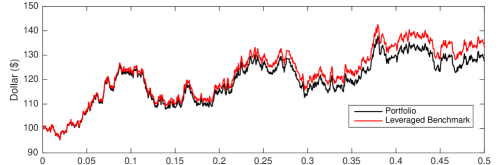
(b) $\beta=2$

(c) $\beta=3$

Figure 2: Sample paths of portfolio values (in $) compared to their benchmarks for (a) $\beta=-1$, (b) $\beta=2$, and (c) $\beta=3$ under the Black-Scholes model. Parameters: $X_{0}=100$, $S_{0}$, $r=0.05$, $\sigma=0.2$, and $T=0.5$. The benchmark is defined such that its log-return is equal to $\beta$ times the index’s log-return, with an initial value of $\$100$.

The associated strategy achieving such path properties requires the use of at least $d+1=1$ derivative. Using exactly $1$ leads to a unique strategy. To find the unique strategy, we can (without loss of generality) solve the corresponding equation in (2.10) to get $w_{t}=\beta/D_{t}$. Let us compare the tracking strategies using call options and futures contracts. First, consider a call on the index with expiration date $T_{c}$ and strike $K$. Its price is given by the Black and Scholes (1973) formula

$$c_{t}:=c(t,S_{t})=S_{t}N\left(d_{+}(t,S_{t})\right)-Ke^{-r(T_{c}-t)}N\left(d_{-}(t,S_{t})\right),$$

where

$$d_{\pm}(t,S_{t}) =\frac{\log\left(S_{t}/K\right)+(r\pm\frac{\sigma^{2}}{2})(T_{c}-t)}{\sigma\sqrt{T_{c}-t}},\quad N(x)=\int_{-\infty}^{x}\frac{1}{\sqrt{2\pi}}e^{-\frac{u^{2}}{2}}du.$$

Therefore, to obtain an exposure coefficient of $\beta$ to the index returns, requires holding

$$\frac{w_{t}X_{t}}{c_{t}}=\frac{\beta X_{0}}{S_{0}}\left(\frac{S_{t}}{S_{0}}\right)^{\beta-1}e^{(r+\frac{\beta\sigma^{2}}{2})(1-\beta)t}\frac{1}{N\left(d_{+}(t,S_{t})\right)}$$ (3.4)

units of call option at time $t$.

The price of a futures written on $S$ with maturity $T_{f}$ is given by $f_{t}:=f(t,S_{t})=S_{t}e^{r(T_{f}-t)}$ for $t\leq T_{f}$. Therefore, to achieve an exposure with coefficient $\beta$ requires holding

$$\frac{w_{t}X_{t}}{f_{t}}=\frac{\beta X_{0}}{S_{0}}\left(\frac{S_{t}}{S_{0}}\right)^{\beta-1}e^{(r+\frac{\beta\sigma^{2}}{2})(1-\beta)t-r(T_{f}-t)}.$$ (3.5)

contracts at time $t$.

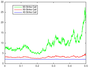
(a) Options

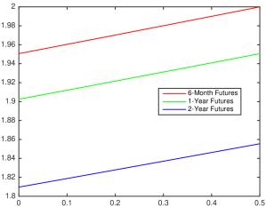
(b) Futures

Figure 3: Simulations of tracking strategies when using (a) a call option of different strike $K\in\left\{40,50,60\right\}$ and $T_{c}=0.5$, and (b) futures with maturity $T_{f}\in\left\{0.5,1,2\right\}$ under the Black-Scholes model. Parameters: $S_{0}=50$, $X_{0}=100$, $r=0.05$, $\sigma=0.2$, and $T=0.5$.

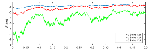
(a) Options

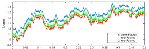
(b) Futures

Figure 4: Simulation of tracking strategies for (a) call options of various strikes ($K\in\left\{40,50,60\right\}$ and $T_{c}=0.5$) and (b) futures contracts of various maturities ($T_{f}\in\left\{0.5,1,2\right\}$). These strategies target $\beta=-1$ over the trading horizon until $T=0.5$. Parameters are $S_{0}=50$, $X_{0}=100$, $r=0.05$ and $\sigma=0.2$. For the ease of comparison, the strategies are based on sample path of the reference index used in Figure 2.

To gain further intuition, let us compare the above strategies when the investor seeks a unit exposure ($\beta=1$) with respect to $S$. The corresponding futures and options holdings are, respectively,

$$\frac{X_{0}}{S_{0}}e^{-r(T_{f}-t)}\qquad\text{and}\qquad\frac{X_{0}}{S_{0}N\left(d_{+}(t,S_{t})\right)}\,.$$

First, these strategies can be viewed as the reciprocal of the associated delta hedge. Under this model, both calls and futures allow for perfect tracking of $S$, since $\beta=1$ implies that $\alpha=0$. However, the two strategies are very different.

With a call option, the strategy is stochastic, depending crucially on the index dynamics. In Figure 3(a), we display the hedging strategies for call options of strikes $K\in\left\{40,50,60\right\}$ with a common maturity equal to the end of the trading horizon (6 months). The fluctuation of each strategy depends on the moneyness of the option. When $S_{t}>>K$, $N(d_{+}(t,S_{t}))$ is close to $1$ and movements in the call price mimic those in the underlying equity index. As s result, the strategy is roughly constant over time as shown by the bottom path in Figure 3(a). In contrast, if the option used is deep out-of-the-money ($S_{t}<<K$), then $N(d_{+}(t,S_{t}))$ is close to $0$, meaning that the investor needs to hold many units of this call, whose per-unit price is almost zero in such a scenario, to gain sufficient direct exposure to the index $S$. Consequently, small movements can lead to very large changes in the holdings over time (see the top path in Figure 3).

For the futures, even though the contract value is stochastic, the strategy is time-deterministic with position becomes increasingly long exponentially over time at the risk-free rate. In Figure 3(a), we compare the positions corresponding to the futures contracts with different maturities, and notice that tracking with a shorter-term futures requires more units of futures in the portfolio.

Figure 4 displays the strategies for “inverse tracking” portfolios with exposure coefficient $\beta=-1$. As expected, short positions are used, but the option strategy is most (resp. least) stable when the option is most in (resp. out of) the money ($K=40$). The futures strategy is no longer time-deterministic, though the position still shows an increasing trend towards maturity. In fact, the stochastic futures strategy is now proportional to $S^{-2}$, as seen in (3.5) when $\beta=-1$. Comparing across maturities, the shortest-term (resp. longest-term) futures has the most (least) short position, but the position remains negative for all maturities.

3.2 Heston Model

We now discuss the tracking problem under the Heston (1993) model for the equity index. Under the risk-neutral measure, the dynamics of the reference index and stochastic volatility factor are given by

$$dS_{t} =rS_{t}dt+\sqrt{Y_{t}}S_{t}dB_{t}^{{\mathbb{Q}},0}$$

$$dY_{t} =\widetilde{\kappa}(\widetilde{\theta}-Y_{t})dt+\nu\big{(}\rho\sqrt{Y_{t}}dB_{t}^{{\mathbb{Q}},0}+\sqrt{1-\rho^{2}}\sqrt{Y_{t}}dB_{t}^{{\mathbb{Q}},1}\big{)},$$

where $B_{t}^{{\mathbb{Q}},0}$ and $B_{t}^{{\mathbb{Q}},1}$ are two independent SBMs and $\rho\in(-1,1)$ is the instantaneous correlation parameter. The stochastic volatility factor $Y$ is not traded and is driven by a Cox-Ingersoll-Ross (CIR) process. If we assume the Feller condition $2\widetilde{\kappa}\widetilde{\theta}\geq\nu^{2}$ (see Feller (1951)) and $Y_{0}>0$, then $Y$ stays strictly positive at all times almost surely under the risk-neutral measure.

Under the Heston Model, the tracking condition (2.12) becomes

$$\alpha_{t}=r(1-\beta_{t})-\widetilde{\kappa}\left(\frac{\widetilde{\theta}}{Y_{t}}-1\right)\eta_{t},\qquad 0\leq t\leq T.$$

The portfolio is subject to the stochastic drift $\alpha_{t}$ which does not vanish as long as $\eta_{t}\neq 0$ and $\beta_{t}\neq 1$. Therefore, perfect tracking is not achievable.

Let us set the coefficients to be constant, i.e. $\beta_{t}=\beta$ and $\eta_{t}=\eta$ for all $t\in[0,T]$. In the Heston Model, a portfolio generally needs at least $d+1=2$ derivatives to control risk exposure with respect to the two sources of randomness. We solve for the index exposure $\beta$ and factor exposure $\eta$ from the $2\times 2$ system:

$$\left(\begin{array}[]{c}\beta\\ \eta\\ \end{array}\right)=\left(\begin{array}[]{cc}D_{t}^{(1)}&D_{t}^{(2)}\\ E_{t}^{(1)}&E_{t}^{(2)}\\ \end{array}\right)\left(\begin{array}[]{c}w_{t}^{(1)}\\ w_{t}^{(2)}\end{array}\right).$$

The second superscript is suppressed on the factor elasticities since there is only one exogenous factor here. By a simple inversion, the portfolio weights are

$$w_{t}^{(1)}=\frac{\beta E_{t}^{(2)}-\eta D_{t}^{(2)}}{D_{t}^{(1)}E_{t}^{(2)}-D_{t}^{(2)}E_{t}^{(1)}},\qquad w_{t}^{(2)}=\frac{-\beta E_{t}^{(1)}+\eta D_{t}^{(1)}}{D_{t}^{(1)}E_{t}^{(2)}-D_{t}^{(2)}E_{t}^{(1)}}.$$ (3.6)

Of course, this solution is only valid if

$${D_{t}^{(1)}E_{t}^{(2)}\neq D_{t}^{(2)}E_{t}^{(1)}}.$$ (3.7)

For instance, using two European call (or put) options on $S$ with different strikes can lead to the trading strategy that generates the desired exposure associated with the given coefficients $\beta$ and $\eta$. However, issues may arise when only futures are used, as we will discuss next.

Example 3.1

Using two futures on $S$, with maturities $T_{f}^{(k)}$ ($k=1,2$), the corresponding portfolio weights are given by

$$u_{t}^{(1)}=\frac{\beta H_{t}^{(2)}-\eta G_{t}^{(2)}}{G_{t}^{(1)}H_{t}^{(2)}-G_{t}^{(2)}H_{t}^{(1)}},\quad\text{and}\quad u_{t}^{(2)}=\frac{-\beta H_{t}^{(1)}+\eta G_{t}^{(1)}}{G_{t}^{(1)}H_{t}^{(2)}-G_{t}^{(2)}H_{t}^{(1)}},$$ (3.8)

provided that ${G_{t}^{(1)}H_{t}^{(2)}\neq G_{t}^{(2)}H_{t}^{(1)}}$. Since the futures prices are $f_{t}^{T_{k}}=S_{t}e^{r(T_{f}^{(k)}-t)}$, for $k=1,2$, the elasticities (see (2.29)-(2.30)) simplify to

$$G_{t}^{(k)} =\frac{S_{t}}{f_{t}^{T_{f}^{(k)}}}\frac{\partial f^{T_{f}^{(k)}}}{\partial S}=1,\quad\text{and}\quad H_{t}^{(k)} =\frac{Y_{t}}{f_{t}^{T_{f}^{(k)}}}\frac{\partial f^{T_{f}^{(k)}}}{\partial Y}=0.$$

However, this means that ${G_{t}^{(1)}H_{t}^{(2)}=G_{t}^{(2)}H_{t}^{(1)}}=0$, so the strategy in (3.8) is not well defined. Hence, it is generally impossible to construct a futures portfolio that generates the desired exposure with respect to both the index and stochastic volatility factor for any non-zero coefficients $\beta$ and $\eta$.

As shown in Example 3.1, in order to gain exposure to $S$ and $Y$, the derivative need to have a non-zero sensitivity with respect to $Y$. If the investor does not seek exposure to $Y$ (i.e. $\eta=0$), then she only needs a single futures on $S$ to obtain the corresponding volatility-neutral portfolio. Next, we show that by including a futures on $Y$ we obtain a tracking portfolio that can generate any desired exposure to $S$ and $Y$.

Example 3.2

The Heston model can be viewed as a joint model for the market index and volatility index. The CIR process has also been used to model the volatility index due to their common mean-reverting property (see Grübichler and Longstaff (1996) and Mencía and Sentana (2013), among others). Suppose there exist a futures on the market index $S$ as well as a futures on the volatility index $Y$, and consider a dynamic portfolio of these two futures contracts. We use the superscript $1$ to indicate the futures on the index (of maturity $T_{f}$) and the superscript $2$ to indicate the futures on the variance process (of maturity $T_{y}$). The prices of the $T_{f}$-futures on $S$ and the $T_{y}$-futures on $Y$ are respectively given by

$$f_{t}^{T_{f}}=S_{t}e^{r(T_{f}-t)}\quad\text{ and }\quad g^{T_{y}}_{t}=Y_{t}e^{-\widetilde{\kappa}(T_{y}-t)}+\widetilde{\theta}(1-e^{-\widetilde{\kappa}(T_{y}-t)}).$$

The relevant price elasticities are

$$G_{t}^{(1)}=1,\quad H_{t}^{(1)}=0,\quad G_{t}^{(2)}=0,\quad\text{and}\quad H_{t}^{(2)}=\frac{Y_{t}}{g^{T_{y}}_{t}}e^{-\widetilde{\kappa}(T_{y}-t)}.$$

The strategy $(u_{t}^{(1)},u_{t}^{(2)})$ achieving the exposure with coefficients $\beta$ and $\eta$ is found from the system:

$$\left(\begin{array}[]{c}\beta\\ \eta\\ \end{array}\right)=\left(\begin{array}[]{cc}G_{t}^{(1)}&G_{t}^{(2)}\\ H_{t}^{(1)}&H_{t}^{(2)}\\ \end{array}\right)\left(\begin{array}[]{c}u_{t}^{(1)}\\ u_{t}^{(2)}\end{array}\right).$$

The system admits a unique solution, yielding the portfolio weights:

$$u_{t}^{(1)}=\beta,\quad\text{and}\quad u_{t}^{(2)}=\eta+\eta\frac{\widetilde{\theta}}{Y_{t}}\left(e^{\widetilde{\kappa}(T_{y}-t)}-1\right).$$

Interestingly, the portfolio weight $u_{t}^{(1)}$ (resp. $u_{t}^{(2)}$) depends only on $\beta$ (resp. $\eta$).

Finally, we discuss the slippage process under the Heston model. Applying Proposition 2.2, we obtain

$$Z_{t}=r-r\beta-\widetilde{\kappa}\left(\frac{\widetilde{\theta}}{Y_{t}}-1\right)\eta+\frac{1}{2}\beta(1-\beta)Y_{t}+\frac{1}{2}\eta(1-\eta)\frac{\nu^{2}}{Y_{t}}-\beta\eta\nu\rho.$$ (3.9)

The term $\frac{1}{2}\beta(1-\beta)Y_{t}$ in (3.9) indicates that the current slippage $Z_{t}$ depends on the instantaneous variance $Y$ of the index $S$. Similarly, the term $\frac{1}{2}\eta(1-\eta)\frac{\nu^{2}}{Y_{t}}$ reflects the dependence of the slippage on the instantaneous variance of the stochastic volatility $Y$. As in the Black-Scholes case, for $\eta\notin[0,1]$, this term is negative. The final term $-\beta\eta\nu\rho$ is the instantaneous covariance between the index and the stochastic volatility. Since $\nu>0$, the term is positive whenever $\beta\eta\rho<0$. This happens either when (i) all three are negative, or (ii) exactly 1 is negative. Since equity returns and volatility are typically negatively correlated ($\rho<0$), so going long on both the index and stochastic volatility ($\beta,\eta>0$) can generate positive returns. This covariance term can offset some losses due to volatility decay.

4 Volatility Index Tracking

In this section, we discuss tracking of the volatility index, VIX, under two continuous-time models. These models were first applied to pricing volatility futures and options by Grübichler and Longstaff (1996) and Mencía and Sentana (2013), among others. We expand their analysis to understand the tracking performance of VIX derivatives portfolios and VIX ETFs.

4.1 CIR Model

The volatility index, denoted by $S$ in this section, follows the CIR process:

$$dS_{t}=\widetilde{\kappa}\left(\widetilde{\theta}-S_{t}\right)dt+\sigma\sqrt{S_{t}}dB^{\mathbb{Q}}_{t},$$ (4.1)

with constant parameters $\widetilde{\kappa},\widetilde{\theta},$ and $\sigma>0$. If we assume the Feller condition $2\widetilde{\kappa}\widetilde{\theta}\geq\sigma^{2}$ (see Feller (1951)) and $S_{0}>0$, then $S$ stays strictly positive at all times almost surely. We omit the second superscript on the SBM $B_{t}^{\mathbb{Q}}$ since there is only one SBM in this model.

Under the CIR model, the tracking condition from (2.12) becomes

$$\alpha_{t}=r-\beta_{t}\widetilde{\kappa}\left(\frac{\widetilde{\theta}}{S_{t}}-1\right),$$ (4.2)

for all $t\in[0,T]$. Therefore, for any given exposure coefficient $\beta_{t}$, there is a non-zero stochastic drift depending on the inverse of $S_{t}$. In particular, if $\beta_{t}=0$, then $\alpha_{t}=r$ and we recover the risk free rate by eliminating exposure to the volatility index. Next, suppose $\beta_{t}=1$ for a $100\%$ exposure to the volatility index. Then, the stochastic drift takes the form

$$\alpha_{t}=\frac{\left(\widetilde{\kappa}+r\right)S_{t}-\widetilde{\kappa}\widetilde{\theta}}{S_{t}},$$ (4.3)

which is negative (resp. positive) whenever $S_{t}$ is iss below (resp. above) the critical level $\frac{\widetilde{\kappa}\widetilde{\theta}}{\widetilde{\kappa}+r}$. In addition, if $r=0$, then the critical value is equal to $\widetilde{\theta}$. Then, as $S_{t}$ mean-reverts to $\widetilde{\theta}$, the drift is on average equal to $0$, but is stochastic nonetheless.

Furthermore, according to Proposition 2.2, the slippage process given any constant $\beta\in{\mathbb{R}}$ in the CIR Model is given by

$$Z_{t} =r-\beta\widetilde{\kappa}\left(\frac{\widetilde{\theta}}{S_{t}}-1\right)+\frac{1}{2}\beta(1-\beta)\frac{\sigma^{2}}{S_{t}}.$$

The second term reflects the mean reverting path behavior of $S$. And since $\widetilde{\theta}$ is the long-run mean of $S_{t}$, this term is expected to stay around zero over time, though the deviation from zero is proportional to $\beta\widetilde{\kappa}$. The last term involves the variance of the volatility index, $\frac{\sigma^{2}}{S_{t}}$, and is strictly negative for $\beta\notin[0,1]$, leading to value erosion. Lastly, we observe that $Z_{t}$ is an affine function of ${S_{t}}^{-1}$, which is an inverse CIR process. The moments and other statistics of such a process are well known (see Ahn and Gao (1999)), so this form will be useful for understanding the distribution and computing expectations of $Z_{t}$.

Since there are $d=0$ factors outside of the volatility index, $d+1=1$ derivatives allow for a unique tracking strategy. Specifically, we study the dynamics of portfolios of futures written on $S$. For any maturity $T$, the futures price is

$$f^{T}_{t}:=f(t,S,T)={\mathbb{E}}^{{\mathbb{Q}}}\left[S_{T}|S_{t}=S\right]=(S-\widetilde{\theta})e^{-\widetilde{\kappa}(T-t)}+\widetilde{\theta}.$$ (4.4)

In Figure 5 we display two term structures of VIX futures on two different dates, calibrated to the CIR model. The term structure can be either increasing concave or decreasing convex (see e.g. Li (2016) and Chap 5 of Leung and Li (2016).) While the good fits further suggest that the CIR Model is a suitable model for VIX, we remark that there exist examples of irregularly shaped VIX term structures and calibrated model parameters often change over time. This motivates us to investigate the tracking problem under a more sophisticated VIX model in the next section.

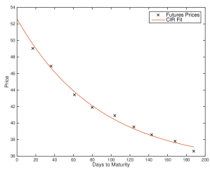
(a) Feb. 23, 2009

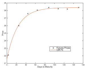
(b) Dec. 11, 2009

Figure 5: Term structure of VIX futures as observed on (a) Feb. 23, 2009 and (b) Dec. 11, 2009. The term structure has changed from decreasing convex to increasing concave.

The futures trading strategy is given by

$$u_{t}=\beta+\frac{\beta\widetilde{\theta}}{S_{t}}\left(e^{\widetilde{\kappa}(T-t)}-1\right).$$ (4.5)

Of course, one may set $\beta=1$ to seek direct exposure to the volatility index. A number of VIX ETFs/ETNs attempt to gain direct exposure to VIX (e.g. VXX) by constructing a futures portfolios with time-deterministic weights. The following example elucidates how and to what extent such an exchange-traded product falls short of this goal.

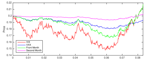
Figure 6: Simulation of VXX along with VIX and the two futures contracts VXX holds over 1 month ($T=1/12$). Parameters are $S_{0}=0.2$, $\widetilde{\kappa}=20$, $\widetilde{\theta}=0.2$ and $\nu=0.4$.

4.2 Comparison to VXX

Let us consider a portfolio of futures with a time-deterministic strategy. Its value evolves according to

$$\frac{dV_{t}}{V_{t}}=u(t)\frac{df^{T_{i(t)}}_{t}}{f^{T_{i(t)}}_{t}}+(1-u(t))\frac{df^{T_{i(t)+1}}_{t}}{f^{T_{i(t)+1}}_{t}}+rdt,$$ (4.6)

where $i(t):=\min\{i:T_{i-1}<t\leq T_{i}\}$, $T_{0}:=0$, and the portfolio weight for the $T_{i}$-futures is

$$u(t):=\frac{T_{i(t)}-t}{T_{i(t)}-T_{i(t)-1}}.$$ (4.7)

This is the strategy employed by the popular VIX ETN, iPath S&P 500 VIX Short-Term Futures ETN (VXX). The strategy starts by investing 100% in the front-month VIX futures contract, and decreases its holding linearly from 100% to 0% while the weight on the second-month contract increases linearly from 0% to 100%.

Figure 6 illustrates such a portfolio with simulated index prices. Specifically, we plot the VIX in red, and the VXX price in blue over one month. The component futures (front and second month) are plotted in green and purple (respectively). Compared to the VIX, the VXX is significantly less volatile. This can be confirmed analytically since

$$\left(\frac{dV_{t}}{V_{t}}\right)^{2}=\left(\frac{u(t)}{S_{t}+\widetilde{\theta}(e^{\widetilde{\kappa}(T_{i(t)}-t)}-1)}+\frac{1-u(t)}{S_{t}+\widetilde{\theta}(e^{\widetilde{\kappa}(T_{i(t)+1}-t)}-1)}\right)^{2}(dS_{t})^{2}<\left(\frac{dS_{t}}{S_{t}}\right)^{2},$$

where the inequality is due to $\widetilde{\kappa}(T_{j}-t)>0$ so that $\widetilde{\theta}\left(e^{\widetilde{\kappa}(T_{j}-t)}-1\right)>0$ for any $j$. As seen in Figure 7(a), both VXX and the dynamic portfolio cannot perfectly track VIX over time. Nevertheless, compared to VXX, the dynamic portfolio is more reactive to changes in VIX. In Figure 7(b), we plot two scatterplots of the annualized returns between the dynamic portfolio and VIX (top) and between VXX and VIX (bottom). On both plots, a solid straight line with slope 1 is a drawn for comparison. The dynamic portfolio, while not tracking VIX perfectly, generates highly similar returns as VIX, and is visibly much closer to VIX than VXX.

.

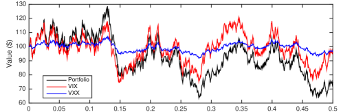
(a) Portfolio Evolution

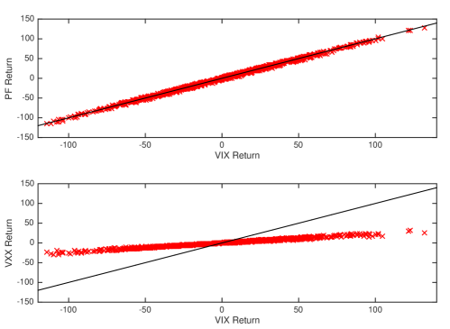
(b) Return Scatter Plots

Figure 7: Sample paths of VIX, VXX, and the dynamic portfolio with $\beta=1$ over a 6-month period ($T=0.5$). Parameters are $S_{0}=0.2$, $\widetilde{\kappa}=20$, $\widetilde{\theta}=0.2$, and $\nu=0.4$. Panel (a) displays the time series of the portfolio value, along with the price paths of VIX and VXX, over time starting at $$100$. Panel (b) shows the scatter plots of the annualized returns between the portfolio and VIX (top) and between VXX and VIX (bottom). On both plots, a solid straight line with slope 1 is a drawn for visual comparison.

Given the VXX strategy (or any other strategy), we can infer from the SDE of the portfolio (see (4.6)) the corresponding drift (the $dt$ term) and exposure to $S$ (coefficient of $dS_{t}/S_{t}$), which we denote by $\alpha_{t}^{(V)}$ and $\beta_{t}^{(V)}$, respectively. As a point of reference, if a portfolio tracks VIX one-to-one perfectly, then we have $\beta_{t}^{(V)}=1$ and $\alpha_{t}^{(V)}=0$. As our earlier discussion following equation (4.3) indicates, this perfect tracking is impossible, but we still wish to illustrate how much VXX deviates from VIX in terms of the implied values of $\alpha_{t}^{(V)}$ and $\beta_{t}^{(V)}$.

Let us denote $T_{1}$ and $T_{2}$ as the maturities for the front-month and second-month futures, respectively. With the portfolio weights in (4.7), we find from the portfolio’s SDE (4.6) that

$$\alpha_{t}^{(V)} =r+\beta_{t}^{(V)}\widetilde{\kappa}\left(1-\frac{\widetilde{\theta}}{S_{t}}\right),$$

$$\beta_{t}^{(V)} =\frac{S_{t}}{f_{t}^{T_{1}}}e^{-\widetilde{\kappa}(T_{1}-t)}-\frac{tS_{t}e^{\widetilde{\kappa}t}}{T_{1}}\left(\frac{e^{-\widetilde{\kappa}T_{1}}}{f_{t}^{T_{1}}}-\frac{e^{-\widetilde{\kappa}T_{2}}}{f_{t}^{T_{2}}}\right).$$

As expected, we do not have $\beta_{t}^{(V)}=1$ and $\alpha_{t}^{(V)}=0$. Indeed both coefficients are stochastic and depend on the level of $S_{t}$. In Figure 7, we illustrate the sample paths of VIX, VXX, and the dynamic portfolio of two futures with exposure coefficient $\beta=1$. The last portfolio attempts to track VIX one-to-one but must be subjected to a stochastic drift $\alpha_{t}\neq 0$.

In Figure 8, we plot the implied $\alpha$ and implied $\beta$ over time based on the sample path of VXX in Figure 7. The implied $\beta$ for VXX varies significantly over time, and is far from the reference value $1$ (for unit exposure to VIX) all the time. On average the implied $\beta$ fluctuates around $0.23$ over the entire 6 month period. Recall that VXX is a long portfolio of the front-month and second-month futures, starting with a 100% allocation in the front-month at each maturity. Interestingly, as VXX allocates more in the second-month futures over time, the portfolio value reaches its maximum approximately halfway through each contract period, suggesting that concentrating on the shortest-term futures does not imply the closest tracking to the underlying index. In Figure 8(b), we plot the stochastic $\alpha$ in units of annualized basis points for both VXX and the dynamic portfolio with $\beta=1$. For both portfolios, $\alpha$ is not 0 as expected. For the dynamic portfolio with $\beta=1$, the stochastic drift is more volatile than that for VXX, but both are relatively small compared to the returns seen in Figure 7(b).

We conclude this example by discussing the futures trading strategies corresponding to $\beta=1$ (see (4.5)) with either the front-month futures only, or the second-month futures only. Recall that in this model only $d+1=1$ derivative product is necessary to achieve unit exposure ($\beta=1$), but the choice of derivative can lead to a very different portfolio weight over time. To see this, we plot in Figure 9 the sample paths of the two portfolio weights corresponding to the two futures contracts with different maturities. In general, the futures strategies tend to decrease exponentially in each maturity cycle, and become discontinuous at maturities as the portfolio rolls into the new futures contract. The front-month futures strategy decays roughly from 5 to 1 in each cycle. Given that futures price will converge to index price by maturity, it is intuitive that the strategy weight becomes 1 for front-month futures. Intuitively, futures prices are typically less volatile than the index, so leveraging (weights greater than 1) is expected and can in effect increase the portfolio’s volatility to attempt to better track the index. Comparing between the two strategies, using the second-month futures to track VIX leads to significant leveraging.

One of the advantages of futures contracts is the ease of leveraging due to margin requirements. If margin requirements are 20% of notional, then it is possible to achieve $5\times$ leverage. Margin requirements are constantly changing for VIX futures. However, $25\times$ to $30\times$ for the second-month futures is neither typical nor practical. The weights for front-month futures are more in line with feasible leverage that one can attain. Recall that the strategy employed by VXX is a time-deterministic one. Figure 9 further illustrates that stochastic portfolio weights are necessary in order to achieve unit exposure to the volatility index.

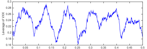
(a) Implied $\beta_{t}$

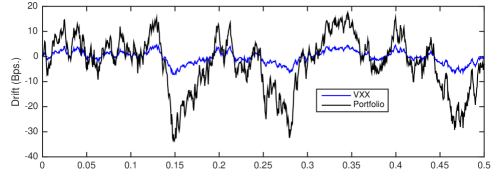
(b) Implied $\alpha_{t}$

Figure 8: With reference to the simulated paths in Figure 7, we show (a) the implied exposure coefficient $\beta_{t}$ inferred from VXX , and (b) stochastic drift $\alpha_{t}$ for both VXX and the tracking portfolio over a six-month period ($T=0.5$).

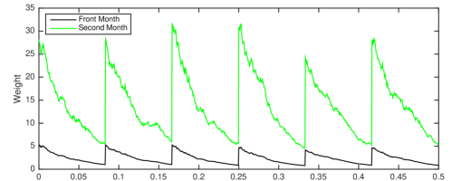
Figure 9: Portfolio weights of the dynamic portfolio with exposure coefficient $\beta=1$ in Figure 7.

4.3 CSQR Model

We now investigate the tracking strategy and slippage process under an extension of the CIR Model. In this section, $S$ will continue to be mean reverting, but the long-run mean is also stochastic. This model is referred to as the concatenated square root process (CSQR) (see Mencía and Sentana (2013)):

$$dS_{t} =\widetilde{\gamma}(Y_{t}-S_{t})dt+\sigma\sqrt{S_{t}}dB_{t}^{{\mathbb{Q}},0},$$

$$dY_{t} =\widetilde{\kappa}(\widetilde{\theta}-Y_{t})dt+\nu\rho\sqrt{Y_{t}}dB_{t}^{{\mathbb{Q}},0}+\nu\sqrt{1-\rho^{2}}\sqrt{Y_{t}}dB_{t}^{{\mathbb{Q}},1}.$$

Here, $B_{t}^{{\mathbb{Q}},0}$ and $B_{t}^{{\mathbb{Q}},1}$ are independent SBMs. We assume the parameters are chosen so that the pair $(S_{t},Y_{t})$ is strictly positive $\forall\,t\geq 0$. Here, the index tends to revert to the stochastic level $Y_{t}$ which is also mean-reverting. This accounts for the empirical observations of the path behavior of VIX, and that VIX futures calibration suggest that the long-run mean oscillates over time (see e.g. Figure 5).

Let the investor set the values of exposure coefficients $\beta_{t}\equiv\beta$ and $\eta_{t}\equiv\eta$, then the portfolio is subject to a stochastic drift (see Proposition 2.1) that is a function of $S_{t}$ and $Y_{t}$:

$$\alpha_{t}=r-\frac{\widetilde{\gamma}(Y_{t}-S_{t})}{S_{t}}\beta-\frac{\widetilde{\kappa}(\widetilde{\theta}-Y_{t})}{Y_{t}}\eta.$$

Also, applying Proposition 2.2, we obtain the slippage process $Z_{t}$ in the CSQR model:

$$Z_{t}=r-\beta\widetilde{\gamma}\left(\frac{Y_{t}}{S_{t}}-1\right)-\eta\widetilde{\kappa}\left(\frac{\widetilde{\theta}}{Y_{t}}-1\right)+\frac{1}{2}\beta(1-\beta)\frac{\sigma^{2}}{S_{t}}+\frac{1}{2}\eta(1-\eta)\frac{\nu^{2}}{Y_{t}}-\frac{\beta\eta\nu\rho\sigma}{\sqrt{S_{t}Y_{t}}}.$$

As we can see, the first two terms reflect the mean-reverting properties of $S_{t}$ and $Y_{t}$. On average, their effects tend to be zero, but are also proportional to the speeds of mean reversion $\widetilde{\gamma}$ and $\widetilde{\kappa}$, and exposure coefficients $\beta$ and $\eta$. The next two terms account for the variances of the index and its stochastic mean, and are negative if $\beta\notin[0,1]$ and $\eta\notin[0,1]$, respectively. The final term reflects the effect of covariance between $S$ and $Y$ in this model. It will be negative if either (i) all three of $\beta,\eta$ and $\rho$ are positive, or (ii) exactly one of $\beta,\eta$, or $\rho$ is positive.

Since $d=1$, we know that $d+1=2$ derivative products are required to obtain the desired exposures. Let us consider the use of futures contracts on $S$. The price of a futures written on $S$ with maturity $T_{k}$ is given by

$$f_{t}^{T_{k}}=\widetilde{\theta}+\left(S_{t}-\widetilde{\theta}\right)e^{-\widetilde{\gamma}(T_{k}-t)}+\begin{cases}\widetilde{\gamma}e^{-\widetilde{\gamma}T_{k}}\left(Y_{t}-\widetilde{\theta}\right)e^{\widetilde{\kappa}t}(T_{k}-t),&\widetilde{\gamma}=\widetilde{\kappa}\\ \frac{\widetilde{\gamma}\left(Y_{t}-\widetilde{\theta}\right)}{\widetilde{\gamma}-\widetilde{\kappa}}\left(e^{-\widetilde{\kappa}(T_{k}-t)}-e^{-\widetilde{\gamma}(T_{k}-t)}\right),&\widetilde{\gamma}\neq\widetilde{\kappa},\end{cases}$$

for $t\leq T_{k}$; see Mencía and Sentana (2013) for a derivation. Notice the first term would be the futures price if $S_{t}$ were reverting to the mean $\widetilde{\theta}$ at speed $\widetilde{\gamma}$. Next we calculate the sensitivities with respect to the index and stochastic mean:

$$\frac{\partial f_{t}^{T_{k}}}{\partial S}=e^{-\widetilde{\gamma}(T_{k}-t)},\quad\text{ and }\quad\frac{\partial f_{t}^{T_{k}}}{\partial Y}=\begin{cases}\widetilde{\gamma}e^{\widetilde{\kappa}t-\widetilde{\gamma}{T_{k}}}({T_{k}}-t),&\widetilde{\gamma}=\widetilde{\kappa}\\ \frac{\widetilde{\gamma}}{\widetilde{\gamma}-\widetilde{\kappa}}\left(e^{-\widetilde{\kappa}({T_{k}}-t)}-e^{-\widetilde{\gamma}({T_{k}}-t)}\right),&\widetilde{\gamma}\neq\widetilde{\kappa}\end{cases}.$$

Henceforth, assume the latter case that $\widetilde{\gamma}\neq\widetilde{\kappa}$. In that case, the respective elasticities are given by

$$G_{t}^{(k)}=\frac{S_{t}}{f_{t}^{{T_{k}}}}e^{-\widetilde{\gamma}({T_{k}}-t)},\quad\text{and}\quad H_{t}^{(k)}=\frac{Y_{t}}{f_{t}^{{T_{k}}}}\frac{\widetilde{\gamma}}{\widetilde{\gamma}-\widetilde{\kappa}}\left(e^{-\widetilde{\kappa}({T_{k}}-t)}-e^{-\widetilde{\gamma}({T_{k}}-t)}\right).$$ (4.8)

Just as in Section 3.2, the second numerical superscript on $H_{t}^{(k)}$ has been suppressed since there is only one exogenous factor in this model.

We consider a portfolio of two futures contracts, both on $S$ with maturities $T_{2}>T_{1}\geq T$. Recall that tracking does not work with two futures in the Heston Model, so one must include another type of derivative (e.g. option). Now in the CSQR model, we check if this futures portfolio works by verifying

$${G_{t}^{(1)}H_{t}^{(2)}\neq G_{t}^{(2)}H_{t}^{(1)}},$$ (4.9)

for all $t\in[0,T]$. Upon plugging in the above elasticities, we find that the condition is equivalent to $T_{1}\neq T_{2}$ (see Appendix A.4.) Since we have assumed that $T_{1}<T_{2}$, the condition holds. Therefore, the linear system of equations

$$\left(\begin{array}[]{c}\beta\\ \eta\\ \end{array}\right)=\left(\begin{array}[]{cc}G_{t}^{(1)}&G_{t}^{(2)}\\ H_{t}^{(1)}&H_{t}^{(2)}\\ \end{array}\right)\left(\begin{array}[]{c}u_{t}^{(1)}\\ u_{t}^{(2)}\end{array}\right),$$ (4.10)

which yields the strategy for the two futures contracts is always solvable.

Soling the system yield the portfolio weights

$$u_{t}^{(1)}=\frac{\beta f_{t}^{T_{1}}}{S_{t}}\left(\frac{e^{\widetilde{\gamma}(T_{2}-t)}-e^{\widetilde{\kappa}(T_{2}-t)}}{e^{\widetilde{\gamma}(T_{2}-T_{1})}-e^{\widetilde{\kappa}(T_{2}-T_{1})}}\right)-\frac{\eta f_{t}^{T_{1}}}{Y_{t}}\left(1-\frac{\widetilde{\kappa}}{\widetilde{\gamma}}\right)\left(\frac{e^{\widetilde{\kappa}(T_{2}-t)}}{e^{\widetilde{\gamma}(T_{2}-T_{1})}-e^{\widetilde{\kappa}(T_{2}-T_{1})}}\right),$$ (4.11)

and

$$u_{t}^{(2)}=\frac{-\beta f_{t}^{T_{2}}}{S_{t}}\left(\frac{e^{\widetilde{\gamma}(T_{1}-t)}-e^{\widetilde{\kappa}(T_{1}-t)}}{e^{-\widetilde{\kappa}(T_{2}-T_{1})}-e^{-\widetilde{\gamma}(T_{2}-T_{1})}}\right)+\frac{\eta f_{t}^{T_{2}}}{Y_{t}}\left(1-\frac{\widetilde{\kappa}}{\widetilde{\gamma}}\right)\left(\frac{e^{\widetilde{\kappa}(T_{1}-t)}}{e^{-\widetilde{\kappa}(T_{2}-T_{1})}-e^{-\widetilde{\gamma}(T_{2}-T_{1})}}\right).$$ (4.12)

For example, take $\beta=1$ and $\eta=0$. Then, only the first terms in (4.11) and (4.12) remain, and $u_{t}^{(1)}$ is positive but $u_{t}^{(2)}$ is negative. This combination of futures contracts allows for direct exposure to the volatility index, without any exposure to the stochastic mean of the volatility.

5 Concluding Remarks

We have studied a class of strategies for tracking an index and generating desired exposure to a given set of factors in a general continuous-time diffusion framework. Our analytical results provide the tracking condition and derivatives trading strategies under any given model. We have illustrated the path-behaviors of the trading strategies and the associated tracking performances under a number of well-known models, such as the Black-Scholes and Heston models for equity tracking, and the CIR and CSQR models for VIX tracking. This has practical implications to investors or fund managers who seek to construct portfolios of derivatives for tracking purposes. Our results also shed light on how tracking errors can arise in a general financial market.

There are many natural and useful extensions to this research. Our illustrative examples include equity indices and volatility indices, but there are many more asset classes, including commodities, fixed income, and currencies. In all these asset classes, many ETFs are designed to track the same or similar indices. There is potential to apply and extend our methodology to analyze the price dynamics and tracking performances of various futures/derivatives-based ETFs, and derivatives portfolios in general. With options written on leveraged ETFs, investors can now use derivatives to generate leveraged exposure. This calls for consistent pricing of LETF options across leverage ratios (see Leung and Sircar (2015); Leung et al. (2016)). Moreover, our work shows that in some models it is impossible to perfectly control exposure to the index and all factors. This should motivate the design of new trading strategies that minimize deviations from a targeted exposure. The insight on tracking errors can in principle be exploited for statistical arbitrage, but it can also help investors and regulators better understand the risks associated with derivatives portfolios.

Appendix A Proofs

A.1 Derivation of SDE (2.5)

By Ito’s formula, the option price satisfies the SDE

$$dc_{t}^{(k)}=\frac{\partial c^{(k)}}{\partial t}dt+dM_{t}^{\intercal}\nabla c^{(k)}+\frac{1}{2}dM_{t}^{\intercal}\nabla^{2}c^{(k)}dM_{t}.$$ (A.1)

Here, the gradient and Hessian are taken with respect to all market variables, $(S,Y^{(1)},...,Y^{(d)})$. We rewrite the last term in (A.1) as follows:

$$dM_{t}^{\intercal}\nabla^{2}c^{(k)}dM_{t} =(\widetilde{\gamma}_{t}dt+\Sigma_{t}dB_{t}^{\mathbb{Q}})^{\intercal}\nabla^{2}c^{(k)}(\widetilde{\gamma}_{t}dt+\Sigma_{t}dB_{t}^{\mathbb{Q}})$$

$$=\left(dB_{t}^{\mathbb{Q}}\right)^{\intercal}\Sigma_{t}^{\intercal}\nabla^{2}c^{(k)}\Sigma_{t}dB_{t}^{\mathbb{Q}}$$

$$=\operatorname{Tr}\left[\left(dB_{t}^{\mathbb{Q}}\right)^{\intercal}\Sigma_{t}^{\intercal}\nabla^{2}c^{(k)}\Sigma_{t}dB_{t}^{\mathbb{Q}}\right]$$

$$=\operatorname{Tr}\left[\Sigma_{t}^{\intercal}\nabla^{2}c^{(k)}\Sigma_{t}dB_{t}^{\mathbb{Q}}\left(dB_{t}^{\mathbb{Q}}\right)^{\intercal}\right]$$

$$=\operatorname{Tr}\left[\Sigma_{t}^{\intercal}\nabla^{2}c^{(k)}\Sigma_{t}\textbf{I}dt\right]=\operatorname{Tr}\left[\Sigma_{t}^{\intercal}\nabla^{2}c^{(k)}\Sigma_{t}\right]dt.$$ (A.2)

Substituting (A.2) into (A.1), we obtain

$$dc_{t}^{(k)}=\left(\frac{\partial c^{(k)}}{\partial t}+\frac{1}{2}\operatorname{Tr}\left[\Sigma_{t}^{\intercal}\nabla^{2}c^{(k)}\Sigma_{t}\right]\right)dt+\frac{\partial c^{(k)}}{\partial S}dS_{t}+\frac{\partial c^{(k)}}{\partial Y^{(1)}}dY_{t}^{(1)}+...+\frac{\partial c^{(k)}}{\partial Y^{(d)}}dY_{t}^{(d)}.$$ (A.3)

On the other hand, the Feynman-Kac formula tells us that the derivative price satisfies

$$\frac{\partial c^{(k)}}{\partial t}+\widetilde{\gamma}_{t}^{(0)}\frac{\partial c^{(k)}}{\partial S}+\widetilde{\gamma}_{t}^{(1)}\frac{\partial c^{(k)}}{\partial Y^{(1)}}+...+\widetilde{\gamma}_{t}^{(d)}\frac{\partial c^{(k)}}{\partial Y^{(d)}}+\frac{1}{2}\operatorname{Tr}\left[\Sigma_{t}^{\intercal}\nabla^{2}c^{(k)}\Sigma_{t}\right]=rc^{(k)},$$ (A.4)

with the terminal condition: $c^{(k)}(T_{k},s,y^{(1)},...,y^{(d)})=h^{(k)}(s,y_{1},...,y_{d})$ for all vectors $(s,y_{1},...,y_{d})$ with strictly positive components. Using (A.3), we have

$$dc_{t}^{(k)} =\left(rc_{t}^{(k)}-\widetilde{\gamma}_{t}^{(0)}\frac{\partial c^{(k)}}{\partial S}-\widetilde{\gamma}_{t}^{(1)}\frac{\partial c^{(k)}}{\partial Y^{(1)}}-...-\widetilde{\gamma}_{t}^{(d)}\frac{\partial c^{(k)}}{\partial Y^{(d)}}\right)dt$$

$$\quad\quad+\frac{\partial c^{(k)}}{\partial S}dS_{t}+\frac{\partial c^{(k)}}{\partial Y^{(1)}}dY_{t}^{(1)}+...+\frac{\partial c^{(k)}}{\partial Y^{(d)}}dY_{t}^{(d)}.$$

Dividing both sides by $c_{t}^{(k)}$ and using the definitions listed in (2.6), we obtain SDE (2.5).

A.2 Validation of (4.9) when $\widetilde{\kappa}=\widetilde{\gamma}$

We now demonstrate that, in the special case of $\widetilde{\kappa}=\widetilde{\gamma}$ under the CSQR model, tracking strategies exist using two futures on $S$ of different maturities. The elasticity with respect to the index is the same as in (4.8); however, the elasticity with respect to the stochastic mean is

$$H_{t}^{(k)}=\frac{Y_{t}}{f_{t}^{T_{k}}}\frac{\partial f_{t}^{T_{k}}}{\partial Y}=\frac{Y_{t}}{f_{t}^{T_{k}}}\widetilde{\gamma}e^{\widetilde{\kappa}t-\widetilde{\gamma}T_{k}}(T_{k}-t).$$ (A.5)

Substituting (A.5) into (4.9), we have

$$\frac{S_{t}}{f_{t}^{T_{1}}}e^{-\widetilde{\gamma}(T_{1}-t)}\frac{Y_{t}}{f_{t}^{T_{2}}}\widetilde{\gamma}e^{\widetilde{\kappa}t-\widetilde{\gamma}T_{2}}(T_{2}-t)\neq\frac{S_{t}}{f_{t}^{T_{2}}}e^{-\widetilde{\gamma}(T_{2}-t)}\frac{Y_{t}}{f_{t}^{T_{1}}}\widetilde{\gamma}e^{\widetilde{\kappa}t-\widetilde{\gamma}T_{1}}(T_{1}-t)$$

$$\iff e^{-\widetilde{\gamma}(T_{1}-t)}e^{\widetilde{\kappa}t-\widetilde{\gamma}T_{2}}(T_{2}-t)\neq e^{-\widetilde{\gamma}(T_{2}-t)}e^{\widetilde{\kappa}t-\widetilde{\gamma}T_{1}}(T_{1}-t)\iff T_{1}\neq T_{2}.$$

Under the assumption that $T_{1}<T_{2}$, the resulting system is solvable and yields strategies that achieve the given exposures.

A.3 Solution to (4.10) when $\widetilde{\kappa}=\widetilde{\gamma}$

With the elasticity with respect to the stochastic mean given by (A.5) and $\widetilde{\kappa}=\widetilde{\gamma}$ under the CSQR model, the portfolio weights that solve system (4.10) are

$$u_{t}^{(1)}=\frac{\beta f_{t}^{T_{1}}}{S_{t}}\left(\frac{e^{\widetilde{\gamma}(T_{1}-t)}(T_{2}-t)}{T_{2}-T_{1}}\right)-\frac{\eta f_{t}^{T_{1}}}{Y_{t}}\left(\frac{e^{\widetilde{\gamma}(T_{1}-t)}}{\widetilde{\gamma}(T_{2}-T_{1})}\right),$$

and

$$u_{t}^{(2)}=\frac{-\beta f_{t}^{T_{2}}}{S_{t}}\left(\frac{e^{\widetilde{\gamma}(T_{2}-t)}(T_{1}-t)}{T_{2}-T_{1}}\right)+\frac{\eta f_{t}^{T_{2}}}{Y_{t}}\left(\frac{e^{\widetilde{\gamma}(T_{2}-t)}}{\widetilde{\gamma}(T_{2}-T_{1})}\right).$$

In particular, take $\beta=1$ and $\eta=0$. Then, the portfolio weights simplify to

$$\ \begin{aligned} u_{t}^{(1)}=\frac{f_{t}^{T_{1}}}{S_{t}}\left(\frac{e^{\widetilde{\gamma}(T_{1}-t)}(T_{2}-t)}{T_{2}-T_{1}}\right),\quad\text{and}\quad u_{t}^{(2)}=\frac{-f_{t}^{T_{2}}}{S_{t}}\left(\frac{e^{\widetilde{\gamma}(T_{2}-t)}(T_{1}-t)}{T_{2}-T_{1}}\right).\\ \end{aligned}$$

By inspection, $u_{t}^{(1)}$ is positive while $u_{t}^{(2)}$ is negative.

A.4 Validation of (4.9) when $\widetilde{\kappa}\neq\widetilde{\gamma}$

We substitute the elasticities from (4.8) into (4.9), and then check directly whether or not the following holds:

$$\frac{S_{t}}{f_{t}^{T_{1}}}e^{-\widetilde{\gamma}(T_{1}-t)}\frac{Y_{t}}{f_{t}^{T_{2}}}\frac{\widetilde{\gamma}}{\widetilde{\gamma}-\widetilde{\kappa}}\left(e^{-\widetilde{\kappa}(T_{2}-t)}-e^{-\widetilde{\gamma}(T_{2}-t)}\right)\neq\frac{S_{t}}{f_{t}^{T_{2}}}e^{-\widetilde{\gamma}(T_{2}-t)}\frac{Y_{t}}{f_{t}^{T_{1}}}\frac{\widetilde{\gamma}}{\widetilde{\gamma}-\widetilde{\kappa}}\left(e^{-\widetilde{\kappa}(T_{1}-t)}-e^{-\widetilde{\gamma}(T_{1}-t)}\right)$$

$$\qquad\qquad\iff e^{-\widetilde{\gamma}T_{1}}\left(e^{-\widetilde{\kappa}(T_{2}-t)}-e^{-\widetilde{\gamma}(T_{2}-t)}\right)\neq e^{-\widetilde{\gamma}T_{2}}\left(e^{-\widetilde{\kappa}(T_{1}-t)}-e^{-\widetilde{\gamma}(T_{1}-t)}\right)\iff T_{1}\neq T_{2}.$$

Since we assume $T_{1}<T_{2}$, the resulting system is solvable and allows for strategies to attain the required exposures.

References

- Ahn and Gao (1999) Ahn, D. and Gao, B. (1999). A parametric nonlinear model of term structure dynamics. The Review of Financial Studies, 12(4):721–762.
- Alexander and Barbosa (2008) Alexander, C. and Barbosa, A. (2008). Hedging index exchange traded funds. Journal of Banking and Finance, 32(2):326–337.
- Alexander and Korovilas (2013) Alexander, C. and Korovilas, D. (2013). Volatility exchange-traded notes: Curse or cure? The Journal of Alternative Investments, 16(2):52–70.
- Avellaneda and Zhang (2010) Avellaneda, M. and Zhang, S. (2010). Path-dependence of leveraged ETF returns. SIAM Journal of Financial Mathematics, 1(1):586–603.
- Black (1976) Black, F. (1976). Studies of stock price volatility changes. In Proceedings of the 1976 Meetings of the American Statistical Association, Business and Economics Statistics Section, pages 177–181.
- Black and Scholes (1973) Black, F. and Scholes, M. (1973). The pricing of options and corporate liabilities. The Journel of Political Economy, 81(3):637–654.
- Cox et al. (1985) Cox, J. C., Ingersoll, J. E., and Ross, S. A. (1985). A theory of the term structure of interest rates. Econometrica, 53(2):385–408.
- Deng et al. (2012) Deng, G., McCann, C., and Wang, O. (2012). Are VIX futures ETPs effective hedges? The Journal of Index Investing, 3(3):35–48.
- Duffie and Kan (1996) Duffie, D. and Kan, R. (1996). A yield-factor model of interest rates. Mathematical Finance, 6(4):379–406.
- Edirisinghe (2013) Edirisinghe, N. C. P. (2013). Index-tracking optimal portfolio selection. Quantitative Finance Letters, 1(1):16–20.
- Feller (1951) Feller, W. (1951). Two singular diffusion problems. The Annals of Mathematics, 54(1):173–182.
- Grübichler and Longstaff (1996) Grübichler, A. and Longstaff, F. (1996). Valuing futures and options on volatility. Journal of Banking and Finance, 20(6):985–1001.
- Guo and Leung (2015) Guo, K. and Leung, T. (2015). Understanding the tracking errors of commodity leveraged ETFs. In Aid, R., Ludkovski, M., and Sircar, R., editors, Commodities, Energy and Environmental Finance, Fields Institute Communications, pages 39–63. Springer.
- Heston (1993) Heston, S. L. (1993). A closed-form solution for options with stochastic volatility with applications to bond and currency options. Review of Financial Studies, 6(2):327–343.
- Husson and McCann (2011) Husson, T. and McCann, C. (2011). The VXX ETN and volatility exposure. PIABA Bar Journal, 18(2):235–252.
- Jarrow (2010) Jarrow, R. (2010). Understand the risks of leveraged ETFs. Finance Research Letters, 7(3):135–139.
- Leung and Li (2016) Leung, T. and Li, X. (2016). Optimal Mean Reversion Trading: Mathematical Analysis and Practical Applications. World Scientific, Singapore.
- Leung et al. (2016) Leung, T., Lorig, M., and Pascucci, A. (2016). Leveraged ETF implied volatilities from ETF dynamics. Mathematical Finance.
- Leung and Santoli (2016) Leung, T. and Santoli, M. (2016). Leveraged Exchange-Traded Funds: Price Dynamics and Options Valuation. Springer Briefs in Quantitative Finance, Springer.
- Leung and Sircar (2015) Leung, T. and Sircar, R. (2015). Implied volatility of leveraged ETF options. Applied Mathematical Finance, 22(2):162–188.
- Leung and Ward (2015) Leung, T. and Ward, B. (2015). The golden target: Analyzing the tracking performance of leveraged gold ETFs. Studies in Economics and Finance, 32(3):278–297.
- Li (2016) Li, J. (2016). Trading VIX futures under mean reversion with regime switching. International Journal of Financial Engineering, 03(03):1650021.
- Mencía and Sentana (2013) Mencía, J. and Sentana, E. (2013). Valuation of VIX derivatives. Journal of Financial Economics, 108(2):367–391.
- Primbs and Sung (2008) Primbs, J. and Sung, C. (2008). A stochastic receding horizon control approach to constrained index tracking. Asia-Pacific Financial Markets, 15(1):3–24.
- Whaley (2013) Whaley, R. E. (2013). Trading volatility: At what cost? Journal of Portfolio Management, 40(1):195–108.
- Yao et al. (2006) Yao, D., Zhang, S., and Zhou, X. (2006). Tracking a financial benchmark using a few assets. Operations Research, 54(4):232–246.